1

Feasibility of ERA5 Integrated Water Vapor trends for climate change

validated by GPS with the consideration of statistical significance: a case study

in Europe

Correspondence to Peng Yuan (peng.yuan@kit.edu)

Abstract

The statistical significance of Integrated Water Vapor (IWV) trends is essential to a correct

interpretation of climate change, but how to properly take it into account remains a challenge.

This study validates the feasibility of ERA5 IWV for climate change in Europe by using the trends

of ground-based GPS hourly IWV series from 1995 to 2017 with the consideration of trend

uncertainty. To obtain realistic IWV trend uncertainties, Autoregressive Moving Average

ARMA(1,1) noise model is proven to be preferred over commonly assumed white noise, first-

order autoregressive noise, etc. GPS IWV offsets validated with improper noise model and

prolonged gaps are found to bias the trend estimation, and thus the affected trend estimates are

unqualified for the validation of ERA5 IWV trends. For the validation at each station, estimating

the trends of the IWV difference time series is more precise than the widely used approach of

calculating the differences between the ERA5 and GPS IWV trends. Weighted Total Least Squares

(WTLS) regression is proposed to be used for the assessments of the overall IWV trend consistency

and the water vapor feedback effect. Unlike commonly used Ordinary Least Squares (OLS), the

WTLS takes account of not only the deviations but also the uncertainties of both independent and

dependent variables, and thus results in a more reasonable regression. The WTLS regression

2

results indicate that the ERA5 and GPS trends are comparable, and both the ERA5 and GPS IWV

to station temperature (IWV–𝑇! ) relationships are in agreement with the prediction of the

Clausius–Clapeyron equation (7% K-1) at 95% confidence level. However, the OLS regression

incorrectly resulted in opposite conclusions on the trend consistency and the GPS IWV–𝑇!

relationship. Therefore, the WTLS regression are recommended to avoid misinterpretation of

climate change.

1 Introduction

As the largest contributor to the global greenhouse effect (~75%), water vapor plays a vital

role in the Earth’s climate change (Lacis et al., 2010). Unlike other greenhouse gases, the amount

of water vapor in the atmosphere is controlled mostly by air temperature (Myhre et al., 2013).

According to the Clausius–Clapeyron (C–C) equation, the water holding capacity of the

atmosphere increases by ~7% with 1 K growth of the air temperature (Trenberth et al., 2003).

Thus, it is considered as a water vapor positive feedback loop that global warming increases the

amount of water vapor in the atmosphere via stronger evaporation, and then the extra water

vapor warms the atmosphere further due to the greenhouse effect (Held and Soden, 2006).

However, the water vapor change rate deviates from the prediction of 7% K-1 when the relative

humidity (RH) does not stay constant. In particular, the RH over land are often reduced by

warming temperature if the surface evaporation is too weak (O’Gorman and Muller, 2010; Wang

et al., 2016). Therefore, an accurate and reliable estimation of IWV trends is of great importance.

3

Despite water vapor is so important for climate change, it is still a challenge to quantify its

trend and the trend uncertainty accurately and reliably. Particularly, it is quite difficult to obtain

long-term homogeneous IWV observations over land where the main humidity data are sourced

from traditional radiosonde, which may suffer from large errors (Dai et al., 2011). Atmospheric

reanalyses are very promising data sources for climate research as they have long-term

continuous data and uniform spatiotemporal resolutions. However, many previous reanalyses

might have been contaminated by unhomogenized radiosonde data, and hence their suitability

for detecting climate trends still remains controversial (Thorne et al., 2010; Dai et al., 2011;

Trenberth et al., 2011; Schröder et al., 2016). As the latest global reanalysis of European Centre

for Medium-Range Weather Forecasts (ECMWF), ERA5 superseded ERA-Interim (ERAI) with a

much higher spatiotemporal resolution ( 0.25° × 0.25° , 1 hour) by using more advanced

modelling and data assimilation systems. However, the feasibility of long-term ERA5 IWV in

climate change is still needed to be assessed.

Ground-based GPS has been widely used as an independent diagnostic tool for validating

reanalyses IWV products as its observations are not assimilated into the reanalyses. However, the

IWV estimates obtained from GPS and reanalyses are often unequal. One possible reason is the

representativeness differences, as GPS is a station point measurement whereas reanalyses are

grid data, (Bock and Parracho, 2019). Moreover, the GPS IWV series might be subjected to

inhomogeneities caused by changes of data processing strategies (e.g. Vey et al., 2009), offsets

triggered by device replacements (e.g. Ning et al., 2016), gaps due to data interruption (Alshawaf

et al., 2018) and so on. While the inhomogeneities due to data processing can be avoided by

reprocessing the whole GPS data with a homogeneous strategy, the offsets and gaps may still bias

4

the GPS IWV trend estimation and thus lead to erroneous conclusions. Therefore, their impacts

should be eliminated or mitigated before the trend validation. Offsets are the systematic shifts of

the series after specific epochs usually caused by antenna/radome changes at the GPS stations.

Estimating offsets and trend simultaneously is an ill-posed problem as they are highly correlated.

Hence, the offsets should be carefully identified with long-term metadata, a proper detection

method, and a reliable significance test (Malderen et al., 2020). Different strategies have been

used for the validation of offsets. For example, Ning et al. (2016) identified the offsets with a

modified penalized maximal t test which accounts for first-order autoregressive (AR(1)) noise in

time series, whereas Klos et al. (2018) evaluated the significance of the offsets by using a 3 ∙ 𝜎

rule with an assumption of white noise (WN). Wang (2008) argued that wrong offsets are very

likely to be identified if the autocorrelation of the time series is ignored. Therefore, the realistic

offsets can only be properly validated based on a comprehensive understanding of the stochastic

properties of the IWV series. However, a proper noise model for the hourly IWV series still needs

to be determined. Gaps, also termed as discontinuities, may also bias the GPS IWV trend

estimation. The gaps are usually interpolated prior to the trend estimation. Various interpolation

methods have been employed to fill in the gaps of the IWV series, such as linear interpolation,

cubic spline interpolation (Wang et al., 2019), and singular spectrum analysis (Wang et al., 2016).

Alshawaf et al. (2018) suggested that the filling algorithms may fail to obtain an unbiased IWV

trend for the series with too long gaps (>1.5 years). However, the impacts of offsets and gaps on

the hourly GPS IWV trend estimation have not been studied extensively.

Apart from the magnitude of the IWV trends, their statistical significance is also vital for a

correct understanding of climate change. To evaluate the uncertainties of the climate trends, a

5

proper noise model should be determined. As climate series are often charactered with strong

autocorrelation, Tiao et al. (1990) suggested using AR(1) model to describe their stochastic

properties. This suggestion has been accepted by many pervious works on the trend estimation

of IWV series derived from satellite measurements (e.g. Mieruch et al., 2008) and reanalyses (e.g.

Alshawaf et al., 2018). However, the optimal noise model of GPS IWV series might be slightly

different from the AR(1) model due to the fact that it contains GPS technical errors in addition to

the atmospheric variability. For instance, Combrink et al. (2007) used the Autoregressive Moving

Average ARMA(1,1) model and Klos et al. (2018) recommended a combination of white noise plus

first-order autoregressive noise (WN+AR(1)) model. Moreover, it is well known that the GPS

Zenith Total Delay (ZTD) is strongly correlated to station coordinate and the GPS coordinate series

is well described by a combination of white noise plus power-law noise (WN+PL) model (Langbein

et al., 2012; Yuan et al., 2018). The facts imply that the WN+PL model might also be suitable for

the GPS IWV series. Furthermore, though many previous works have demonstrated that the trend

uncertainties are underestimated with an assumption of WN, the severities of the

underestimation differ greatly. For example, Alshawaf et al. (2018) reported that the trend

uncertainties of daily ERAI IWV series in Europe estimated with AR(1) are 1.6–2.5 times greater

than those with WN, whereas Klos et al. (2018) argued that the uncertainty ratios between the

WN+AR(1) model and the pure WN model are 5–14 for the multiyear hourly GPS Zenith Wet Delay

(ZWD) series. Owing to the improvement of temporal resolution, ERA5 is also capable to provide

hourly IWV estimates. Therefore, the optimal noise model for the hourly IWV series should be

properly selected, and then the impact of improper noise models on trend uncertainty can be

evaluated. However, this work has not been thoroughly carried out yet.

6

While the realistic IWV trend uncertainties can be achieved, they are seldom considered in

the validation of reanalyses climate trends or in the investigation of climate change. For example,

many studies have used GPS IWV trends to validate reanalyses results by calculating their trend

differences (𝑡𝑟𝑒𝑛𝑑"#$$. = 𝑡𝑟𝑒𝑛𝑑&'().−𝑡𝑟𝑒𝑛𝑑*+,, e.g. Parracho et al., 2018) site-to-site. However,

the uncertainty of the trend difference estimates can be quite large due to the variance

amplification effect ( 𝜎-.//.0&')-1 = 𝜎&'().0&')-1 + 𝜎*+,0&')-1 ), and thus results in unsignificant trend

differences. Moreover, some studies have used linear regression to evaluate the overall

consistency between the reanalyses and IWV GPS trends (e.g. Ning et al., 2016), but the trend

uncertainties were omitted in the estimation of the fitting line by using ordinary least squares

(OLS). Therefore, a comprehensive consistency evaluation approach with proper considerations

on their statistical significance is still lacking. Likewise, the uncertainty information should also be

considered in the linear regression of IWV–𝑇! for the assessment of water vapor feedback effect.

In this study, we use homogeneously reprocessed multidecadal (12–22 years) GPS IWV at

20 European GPS stations to validate the hourly ERA5 IWV series. We focus on answering the

following questions. (1) Which is the optimal noise model for the GPS and ERA5 hourly IWV series?

(2) How is the influence of noise model on the offsets determination and whether it will further

influence the estimation of IWV trend and its uncertainty? (3) How is the impact of gaps on the

IWV trend estimation? (4) How to avoid the variance amplification effect in the comparison of

GPS and IWV trends? (5) Can the overall IWV trend consistency and water vapor feedback effect

be properly evaluated by linear regressions with the consideration of trend uncertainties and are

they statistically in agreement with the corresponding ideal cases?

7

This paper is organized as follows. In section 2, we briefly report the data sets and IWV

calculation methods, present a data screening approach with a robust moving median filter,

describe the models and methods of IWV time series analysis, and introduce the algorithm of

Weighted Total Least Squares (WTLS) regression which considers the deviations and uncertainties

of both independent and dependent variables. In section 3, we compare and select the optimal

noise model, investigate the influences of GPS offsets determination methods on IWV trend

estimation, evaluate the impact of gaps on the IWV trend estimation, validate the feasibility of

ERA5 IWV trends on climate change research, and analyze the water vapor feedback effect in

Europe. At last, we discuss the results in section 4 and conclude the main findings in section 5.

2 Data and methods

2.1 GPS and ERA5 data

In this work, we used the hourly GPS and ERA5 (IWV) series of 20 GPS stations in Europe

and surrounding areas. The GPS observations are from 1995 to 2017 with lengths between 12 and

22 years. The GPS Zenith Total Delay (ZTD) series were derived from a homogeneously

reprocessed GPS solution provided by University of Luxembourg which as originally used for the

Tide Gauge Benchmark Monitoring (TIGA) project (Hunegnaw et al., 2016). The GPS data were

processed with the Bernese software ver. 5.2 (Dach et al., 2015) in a double-differenced network

solution mode. The processing strategies recommended by the International Earth Rotation and

Reference Systems Service (IERS) 2010 conventions (Petit and Luzum, 2010) were generally

followed. The details of the GPS processing strategies have been described in Hunegnaw et al.

(2016), and hence we only give the strategies related to tropospheric delay correction . The

8

tropospheric delay was corrected with the state-of-the-art Vienna Mapping Function 1 (VMF1,

Böhm et al., 2006) and a priori Zenith Hydrostatic Delay (ZHD) derived from ECMWF (Simmons

and Gibson, 2000). The tropospheric ZTD was estimated every hour together with gradients

estimated every 12 hours. The elevation cutoff angle was set as 3°.

Figure 1 Geographical distribution of the GPS stations

As for Numerical Weather Prediction (NWP) model, we used ERA5 hourly pressure level

products (37 levels) of pressure (𝑃), temperature (𝑇), and RH with a horizontal resolution of

0.25° × 0.25° . ERA5 is the state-of-the-art ECMWF reanalysis data set. ERA5 supersedes its

ancestor, ERAI, with the technology advances over the last decade. Compared with ERAI, the

temporal resolution of ERA5 pressure level products have been improved to one hour. Thus, it

provides the opportunity to compare ERA5 and GPS IWV on hourly level without any interpolation

in time domain.

9

2.2 Calculation of IWV

We estimated the pressure (𝑃!), temperature (𝑇!), weighted mean temperature (𝑇2) and

IWV at the location of each of the GPS station by using the hourly ERA5 products. For each GPS

station, we firstly found the four surrounding grid notes in horizontal. Secondly, for each grid note,

we inter-/extrapolated the 𝑃, 𝑇, and 𝑅𝐻 vertical profiles to the height of the GPS station. For

more details on the inter-/extrapolation, please refer to Wang et al. (2005). Thirdly, we obtained

water vapor pressure (𝑒) profile by using the 𝑇 and 𝑅𝐻, and then we calculated the 𝑇2 by using

the following integration (Davis et al., 1985):

𝑇2 =∫ 𝑒𝑇 d𝑧

∫ 𝑒𝑇1 d𝑧

≈∑𝑒3𝑇3∆𝐻3

∑𝑒3𝑇31∆𝐻3

(1)

where 𝑒3 and 𝑇3 denote the average water vapor pressure in hPa and average temperature in K

at the 𝑗th layer of the atmosphere, respectively. ∆𝐻3 denote the atmosphere thickness at the 𝑗th

layer in m, which is the height difference between the 𝑗th and (𝑗 + 1)th level.

Similarly, the ERA5 IWV were integrated as follow:

IWV = B𝑞𝑔 𝑑𝑃 ≈E

𝑞3𝑔3∆𝑃3 (2)

where 𝑞3 and 𝑔3 denote the average specific humidity in kg kg-1 and average local acceleration of

gravity in m s-2 at the 𝑗 th layer of the atmosphere, respectively. ∆𝑃3 denote the pressure

difference between the (𝑗 + 1)th and the 𝑗th level in Pa.

Finally, we interpolated the 𝑃!, 𝑇!, 𝑇2, and IWV from the four surrounding grid notes to the

location of station by using Inverse Distance Weighting (IDW) as given by Jade and Vijayan (2008).

10

Regarding GPS IWV, we firstly estimated ZHD (in mm) by using ERA5 pressure

(Saastamoinen, 1972, Davis et al., 1985):

ZHD = 2.2768𝑃!

1 − 2.66× 1045 ∙ cos(2𝜑!) − 2.8 × 1046ℎ! (3)

where 𝑃!, 𝜑! and ℎ! are the pressure, latitude, and height of the station with units of hPa, rad and

m, respectively.

Then, we can obtain the ZWD:

ZWD = ZTD − ZHD (4)

At last, we calculated the GPS IWV with the following conversion (Bevis et al.1992):

IWV = 𝜅 ∙ ZWD (5)

𝜅 =107

𝑅8 ∙ [𝑘19+𝑘5/𝑇2] (6)

where 𝑅8 is the gas constant for water vapor, 𝑘19 and 𝑘5 are the atmospheric refractivity

constants (Bevis et al., 1994).

2.3 pre-processing of IWV time series

Despite quality control has been implemented in GPS data processing, the GPS IWV series

still suffer from outliers. To remove outliers in the GPS IWV series, we proposed a two-step data

screening strategy based on their characteristics. The first step is a range check by removing the

IWV values outside the range of 0–83 kg m-2, which are obviously errors for this region. The

second step is a robust sliding window median filter. The steps of the filter are as follow. (1)

Obtaining the IWV residuals by calculating the differences between the IWV series and its 30 days

11

sliding window median values. (2) Examining every IWV data point and excluding the outliers

identified with the interquartile range (IQR) rule. The IQR rule is that a data point is regarded as

an outlier if it is outside the range between Q1 − 1.5 ∙ IQR and Q3 + 1.5 ∙ IQR, in which the IQR

is the difference between the 75th percentiles (Q3) and the 25th percentiles (Q1) of the IWV

series. The sliding window median filter was designed since the IWV values are more scattered in

summer than in winter as can be seen in Fig. 2b. The window width was set as 30 days, which is

a balance between the seasonal variations of the IWV series and the number of values used for

the IQR outlier detection. With the consideration of data range, robustness, and seasonal

variations of the discrete degree, this approach is believed better than the classical outlier

detection approach with a 3 ∙ σ rule for the residuals of a least square fitting.

Figure 2 Screening of hourly GPS IWV series at Station ZIMM (Zimmerwald, Switzerland)

12

2.4 IWV time series analysis

To determine the functional and stochastic model for the IWV trend estimation, we

analyzed the stacked spectra of the GPS and ERA5 IWV series as shown in Fig. 3. From Fig. 3, we

can find significant peaks at annual harmonics (up to the 4th) and diurnal harmonics (up to the

12th) which should be considered in the functional model. However, we found that even though

the annual and diurnal harmonics had been considered in the functional model, the spectral peaks

at diurnal harmonics from the 3rd to the 12th did not decrease. Klos et al. (2018) also reported

this phenomenon for hourly GPS ZWD series and they suggested that it is artificial. Therefore,

these high-order diurnal harmonics were not further considered. The functional model for the

IWV series was as follow (Bevis and Brown, 2014):

IWV(𝑡) = IWV: + 𝑣 ∙ (𝑡 − 𝑡:) +E𝐴# ∙ 𝑠𝑖𝑛(𝜔#𝑡 + 𝜑#) +E𝐷3 ∙ 𝑠𝑖𝑛(𝜔3𝑡 + 𝜑3)1

3;<

=

#;<

+E𝑏> ∙ 𝐻(𝑡 − 𝑡>)?!

>;<

(7)

with 𝐻(𝑡 − 𝑡>) = c0, for𝑡 < 𝑡>0.5, for𝑡 = 𝑡>1, for𝑡 > 𝑡>

(8)

where IWV: is the IWV at the reference epoch 𝑡: and 𝑣 is the IWV trend. 𝐴# and 𝜑# are the

amplitude and initial phase of annual harmonics up to the 4th, 𝜔# = 2𝜋/𝜏#, 𝜏# = (1, 1/2, 1/3,

1/4) year. Similarly, 𝐷# and 𝜑# are the amplitude and initial phase of diurnal and semi-diurnal

harmonics, 𝜔3 = 2𝜋/𝜏3, 𝜏3 = (1, 1/2) day. 𝑏> is the offset at epoch 𝑡>. 𝐻(𝑡 − 𝑡>) is a Heaviside

step function used to model the offsets as defined in Equation (8). The last term for offsets was

only employed to the GPS IWV series.

13

Figure 3 Stacked spectra of GPS (a) and ERA5 (b) IWV. Vertical gray lines indicate the first four annual

harmonics and the first twelve diurnal harmonics

The identification of offsets is a great challenge in the trend estimation of GPS IWV series,

as the trend estimates are highly sensitive to the offsets due to collinearity. Hence, all possible

offsets should be carefully identified. In this work, we checked the GPS station log files, labelled

all the epochs of antenna changes, and estimated them together with other terms as shown in

Equation (8). Next, we tested the significance of the offsets with 𝑜𝑓𝑓𝑠𝑒𝑡 > 2 ∙ 𝜎@$$!AB at 95%

confidence level. Then, we excluded the insignificant offsets and repeated the estimation and

significance test until all the rest offsets are significant.

The assumption of stochastic model for the IWV series influences the estimation of IWV

trend uncertainty and thus should be carefully determined. In this work, we examined and

compared several commonly used noise models for the IWV series, such as WN, WN+PL, AR(1),

WN+AR(1), ARMA(1,1), and WN+ARMA(1,1). The time series analysis was carried out by using the

Hector software ver. 1.7.2 (Bos et al., 2019). Hector is a software package specially designed to

estimate the trend of time series with temporal correlated noises. With an assumption of specific

14

noise model, Hector can estimate the model parameters with the Maximum Likelihood

Estimation (MLE) method. The log-likelihood is:

ln(𝐿) = −12 [𝑁 ln

(2𝜋) + ln(det(𝐂)) + 𝐫𝐓𝐂4𝟏𝐫] (10)

where 𝑁 is the number of data points in the time series,𝐫 is the post-fit residuals, and 𝐂 is the

covariance matrix of the assumed noise model. The forms of the covariance matrixes for the noise

models examined in this paper are as follow.

For an assumption of WN, the covariance matrix is:

𝐂𝑾𝑵 = σGH1 𝐈 (11)

where σGH is the noise amplitude of WN and 𝐈 is the identical matrix.

For an assumption of PL, the covariance matrix can be written as (Williams et al., 2003):

𝐂𝑷𝑳 = σKL1 𝐏(𝜅) (12)

where σKL is the noise amplitude of PL and𝜅 is the spectral index. The form for the matrix 𝐏(𝜅)

is introduced by Williams et al. (2003) and thus not repeated here.

For an ARMA(1,1) model given by

𝑋# = 𝜙𝑋#4< + 𝜃𝑍#4< + 𝑍# (13)

where 𝑋# is the observation at epoch 𝑖, 𝜙 is the autoregressive (AR) paramter,𝜃 is the moving-

average (MA) paramter, and 𝑍# is a Gaussian random variable with zero mean and standard

deviation (STD) σM:NM(<,<). The AR(1) model is a special case of ARMA(1,1) with 𝜃 = 0.

Accordingly, the covariance matrix of ARMA(1,1) is expressed as (Combrink et al., 2007):

15

𝑪M:NM(<,<)#,3 = γ(‖𝑖 − 𝑗‖) (14)

with 𝛾(𝜏) =

⎩⎪⎨

⎪⎧ σM:NM(<,<)

1 �1 + (RST)"

<4R"� , for𝜏 = 0

σM:NM(<,<)1 �(𝜑 + 𝜃) + (RST)"R<4R"

� , for𝜏 = 1

𝛾(𝜏 − 1)𝜑, for𝜏 = 2,3, …

(15)

As for the noise combinations of WN+PL, WN+AR(1), and WN+ARMA(1,1), their covariances

are the summations of the covariances of corresponding noise components.

To select the preferred noise model, we employed the values of Bayesian Information

Criterion (BIC, Schwarz 1978) as a criterion:

𝐵𝐼𝐶 = 𝑘 ∙ ln(𝑁) − 2 ∙ ln(𝐿) (16)

where 𝑘 is the number of parameters estimated by the model, 𝑁 is the number of data points in

the time series, ln(𝐿) is the log-likelihood estimated with MLE. The preferred model has the

lowest BIC value.

2.5 Weighted total least squares regression

The approach of least squares is a standard parameter estimation method in regression

analysis to determine the relationship between the dependent and independent variables. Giving

𝑛 data points {𝑥# , 𝑦#} with STD of �𝜎U# , 𝜎V#�, and assuming the regression equation as 𝑦 = 𝑎 ∙ 𝑥 +

𝑏 with the predicted points {𝑥�# , 𝑦�#} on the regression line. The OLS regression is commonly used

but it only takes the residuals of the dependent variable into account by minimizing the objective

function:

16

𝜒1 =E(𝑦# − 𝑦�#)1?

#;<

(17)

The WTLS approach, unlike the OLS, considers the deviations and uncertainties of both the

dependent and independent variables and thus allows for a more reasonable estimation of the

regression. The objective function of the WTLS regression is:

𝜒1 =E�(𝑥# − 𝑥�#)1

𝜎U#1+(𝑦# − 𝑦�#)1

𝜎V#1�

?

#;<

(18)

For more details on the WTLS algorithm, please refer to Krystek and Anton (2007). With the

WTLS algorithm, we can obtain the regression coefficients vector 𝝁 = [𝑎, 𝑏]W and its variance-

covariance matrix 𝚺. Assuming the theoretical value is 𝝁𝒐 = [𝑎�, 𝑏�]W, we performed a Hotelling’s

𝑇1 test to examine whether the estimated regression is statistically in agreement with the

theoretical equation. The null hypothesis is:

𝐻Y: 𝝁 = 𝝁𝒐 (19)

The corresponding Hotelling’s 𝑇1 statistic is:

𝑇1 = (𝝁 − 𝝁𝒐)𝑻𝚺4𝟏(𝝁 − 𝝁𝒐) (20)

The null hypothesis is accepted if:

𝑇1 ≤ 𝜒1,[1 (21)

where 𝛼 = 0.05. If the null hypothesis is accepted, it indicates that the estimated regression

equation statistically agrees with the theoretical value 𝝁𝒐. Otherwise, they differ significantly.

17

3 Results

3.1 Noise analysis

To obtain more realistical IWV trend uncertainties, we investigated six commonly used

noise models, i.e., WN, WN+PL, AR(1), WN+AR(1) , ARMA(1,1), and WN+ARMA(1,1). Then, we

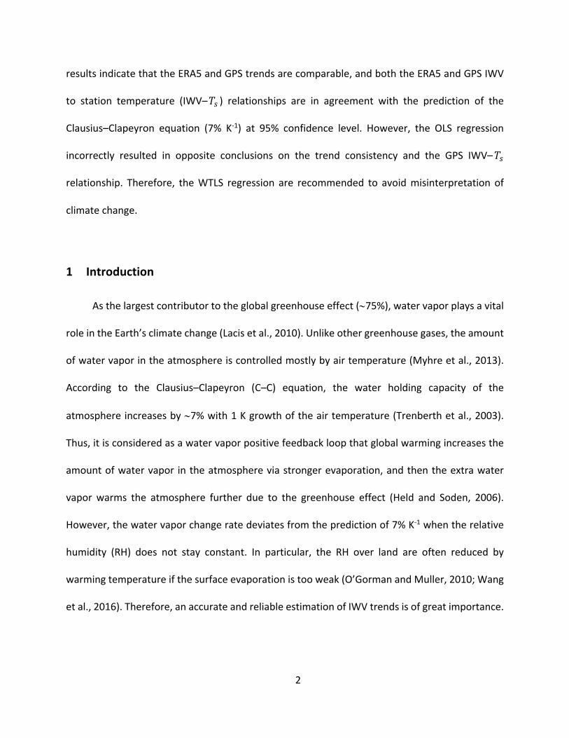
compared and selected the optimal model according to the BIC criterion (Equation (16) and Fig.

4). As can be seen from Fig. 4a, the BIC values of the WN and WN+PL models are the largest,

indicating that they are unsuitable. The BIC values of the WN+AR(1) model are slightly lower than

the values of the AR(1) model, suggesting that including WN to the AR(1) model is beneficial. On

the contrary, the WN+ARMA(1,1) is a bit worse than ARMA(1,1), indicating an

overparameterization. In general, the ARMA(1,1) model has the lowest BIC values and thus it is

selected as the optimal model for the GPS IWV series. Moreover, the BIC values of the WN+AR(1)

model are comparable to those of the ARMA(1,1) model at most stations (17 of 20), which

indicates that it is usually also suitable for the GPS IWV series. Likewise, ARMA(1,1) is also the

optimal model for the ERA5 IWV series (Fig. 4b). However, the WN+AR(1) model is unsuitable for

the ERA5 IWV series, as its BIC values are obviously larger than those of the ARMA(1,1) model.

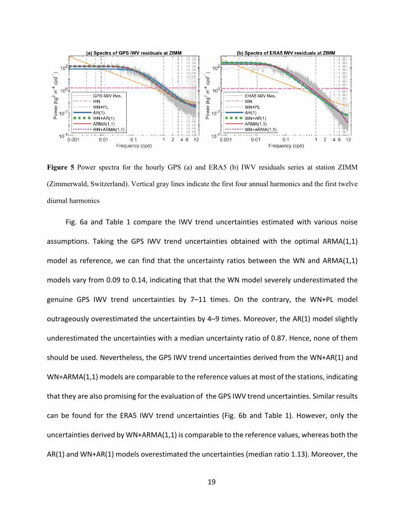
To be more intuitively, Fig. 5 illustrates the power spectra of the hourly GPS and ERA5 IWV

residuals series at station ZIMM (Zimmerwald, Switzerland) together with the spectra of the

various noise assumptions. As shown in Fig. 5a, the spectrum of the GPS IWV residuals stays flat

at low-frequency domain (lower than 0.1 cpd), and then declines sharply at medium-frequency

domain (0.1–2 cpd), and last turn back to flat steadily at high-frequency domain (2–12 cpd).

Whereas the spectrum of WN assumption stays flat at all frequencies and thus fails to fit the

variations of the spectrum of the residuals. Though the spectrum of the WN+PL assumption

18

declines with increasing frequency, it fails to capture the flat GPS IWV residuals spectrum at the

low-frequency domain. Nevertheless, all the AR(1)- and ARMA(1,1)-related models are capable

to describe the characteristics of the GPS IWV residuals spectrum, though the performance of the

pure AR(1) model is slightly worse. Similar results can be found for the ERA5 IWV residuals (Fig.

5b). In particular, the ARMA(1,1) model fits the ERA5 IWV residuals spectrum the best. However,

the spectra of the pure AR(1) model and the WN+AR(1) model are overlapped, which suggests

that including WN to the AR(1) model is meaningless for the ERA5 IWV residuals.

Figure 4 The Bayesian information criterion (BIC) values for GPS (a) and ERA5 (b) IWV series estimated

with various noise assumptions

19

Figure 5 Power spectra for the hourly GPS (a) and ERA5 (b) IWV residuals series at station ZIMM

(Zimmerwald, Switzerland). Vertical gray lines indicate the first four annual harmonics and the first twelve

diurnal harmonics

Fig. 6a and Table 1 compare the IWV trend uncertainties estimated with various noise

assumptions. Taking the GPS IWV trend uncertainties obtained with the optimal ARMA(1,1)

model as reference, we can find that the uncertainty ratios between the WN and ARMA(1,1)

models vary from 0.09 to 0.14, indicating that that the WN model severely underestimated the

genuine GPS IWV trend uncertainties by 7–11 times. On the contrary, the WN+PL model

outrageously overestimated the uncertainties by 4–9 times. Moreover, the AR(1) model slightly

underestimated the uncertainties with a median uncertainty ratio of 0.87. Hence, none of them

should be used. Nevertheless, the GPS IWV trend uncertainties derived from the WN+AR(1) and

WN+ARMA(1,1) models are comparable to the reference values at most of the stations, indicating

that they are also promising for the evaluation of the GPS IWV trend uncertainties. Similar results

can be found for the ERA5 IWV trend uncertainties (Fig. 6b and Table 1). However, only the

uncertainties derived by WN+ARMA(1,1) is comparable to the reference values, whereas both the

AR(1) and WN+AR(1) models overestimated the uncertainties (median ratio 1.13). Moreover, the

20

WN model underestimated the ERA5 IWV trends by 9–14 times (ratios 0.07–0.11). The ERA5 and

GPS IWV trends estimated with the optimal ARMA(1,1) model are listed in Table S1.

Figure 6 GPS (a) and ERA5 (b) IWV trend uncertainties estimated with various noise assumptions

Table 1 Statistics of the ratios between the IWV trend uncertainties estimated with various models and the

optimal ARMA(1,1) model

Models GPS ERA5

Min Median Max Min Median Max WN 0.09 0.11 0.14 0.07 0.09 0.11

WN+PL 3.59 6.94 8.53 2.81 4.21 6.05 AR(1) 0.67 0.87 1.06 0.80 1.13 1.25

WN+AR(1) 1.00 1.00 1.06 0.80 1.13 1.25 WN+ARMA(1,1) 1.00 1.00 1.00 1.00 1.00 1.00

21

Figure 7 Spatial analysis of the ARMA(1,1) noise parameters for the GPS and ERA5 IWV residual series.

(a): GPS AR(1) parameter (𝜙). (b): GPS MA(1) parameter (𝜃). (c): GPS ARMA(1,1) noise amplitude (𝜎).

(d)-(f) are the same as (a)-(c) but for ERA5

Fig. 7 shows the ARMA(1,1) noise parameters for the GPS and ERA5 IWV residual series. The

GPS residual series are characterized with a strong AR process (median: 0.975, IQR: 0.006) and a

weak MA process (median: -0.131, IQR: 0.210). Whereas the ERA5 residual series are

characterized with not only a strong AR process (median: 0.986, IQR: 0.003) but also a strong MA

process (median: -0.630, IQR: 0.086). Moreover, the noise amplitudes of the GPS series (median:

1.22, IQR: 0.19) are larger than those of the ERA5 series (median: 0.49, IQR: 0.15). The noise

characteristics will be discussed in Section 4.1.

22

3.2 Impacts of GPS offsets and gaps

The technique of ground-based GPS usually serves as an independent validation tool for the

IWV derived from reanalyses. However, the GPS IWV itself suffers from various errors. Therefore,

accurate and reliable GPS IWV trend estimates are essential to the validation of ERA5 for climate

change research. In this section, we investigated the impacts of offsets and gaps, two common

problems in GPS IWV series, on the trend estimation of GPS IWV.

As for the validation of offsets, some previous studies tested the significances of the

suspected offsets with an assumption of WN model (e.g. Klos et al., 2018). As the WN model tends

to seriously underestimate the trend uncertainties (Table 1), we suspect whether it also

underestimates the uncertainties of the offset. If so, some unsignificant offsets might be

erroneously identified as significant and then bias the trend estimation. To verify this speculation,

we carried out a control test. The steps are: (1) regarding all the epochs with GPS antenna changes

recorded in the station log files as possible offsets. (2) estimating the offsets, trend, and periodic

signals and confirming the offsets with a significance test at 95% confidence level: 𝑜𝑓𝑓𝑠𝑒𝑡 > 2 ∙

𝜎@$$!AB. (3) excluding the unsignificant offsets and repeating step (2) until all the rest offsets are

significant. (4) estimating the trend, periodic signals, and the significant offsets with an

assumption of ARMA(1,1). The only difference for the control test is in step (2) for the noise model

used in the offset significance test. One experiment used the offset uncertainties estimated with

an assumption of WN in the significance test for simplicity whereas the alternative trial assumed

ARMA(1,1) in the significance test for authenticity. Results show that the assumption of WN

severely underestimated the uncertainties of offsets (5–10 times). Therefore, 33 of the 36

23

suspected offsets are identified as significant with the uncertainties estimated with the WN model,

whereas only 6 are significant when using the uncertainties from the ARMA(1,1) model (Table S2).

Fig. 8 compares the estimates of IWV trend, and its uncertainty derived from the control

test. From Fig. 8 we can find that the simplified offset determination approach does bias the trend

estimation. In particular, the simplified approach results in three negative GPS IWV trends

whereas all the trends are positive when the rigorous approach is applied. Compared with the

rigorous, the simplified approach results in the relative change of the IWV trends by -246% to

196%. It also overestimates the trend uncertainties up to 3 times (station WTZR).

Figure 8 Impact of the offsets determination on IWV trends and their uncertainties (2 ∙ 𝜎) estimated with

ARMA(1,1). The offsets were firstly identified with WN (gray) or identified with ARMA(1,1) (blue)

In practice, GPS IWV series inescapably suffer from gaps. The gaps are data deficiencies at

some epochs of the GPS series due to outliers, equipment failures and so on. To investigate the

impact of gaps on the GPS IWV trend estimation, we performed two simulation experiments. For

the first simulation, we used hourly continuous ERA5 IWV series at the 20 stations from 1995 to

2016. Then, we randomly removed 10%, 20%, and 30% of the observations for each station. At

last, we estimated the IWV trends by using the Hector software with an assumption of ARMA(1,1)

24

model. The Hector software employs linear interpolation approach to interpolate the missing

data. Fig. 9 shows that the estimates of the IWV trends and their uncertainties are almost

unaffected even when 30% of the data are missed randomly.

Figure 9 Comparisons of the IWV trend and its uncertainty (2 ∙ 𝜎) estimates for the ERA5 series from 1995

to 2016 with integration rates of 100%, 90%, 80%, and 70%, respectively

Figure 10 Comparisons of the IWV trend and uncertainty (2 ∙ 𝜎) estimates for the ERA5 series at with and

without gaps with respect to the corresponding GPS IWV series

In addition to the random gaps, GPS IWV series also suffer from prolonged gaps occasionally.

Thus, we designed another simulation in a more realistic case. In this simulation, we extracted

the hourly continuous ERA5 IWV series between the beginning and ending epochs of the

25

corresponding GPS IWV series without gaps. Meanwhile, we extracted the hourly ERA5 IWV series

only at the epochs of the corresponding GPS IWV series. Fig. 10 shows the IWV trends of the two

sets of series. As can be seen from Fig.10, the integration rates of the IWV series range between

71% and 93% with a median of 90%. Comparing the trend uncertainties obtained from the series

with gaps with those without gaps, the relative change ratios range between -9% and 8% with a

median of 0%, indicating that the IWV trend uncertainties are not very sensitive to the gaps, which

is the same as the first simulation with random missing data. However, the relative change ratios

of the IWV trend estimates are much more various with absolute values larger than 50% at three

stations (MORP -182%, REYK 58%, VILL -200%). Nevertheless, all the trend estimates at these

three stations are unsignificant as their values are much smaller than their uncertainties.

In sum, the gap simulations indicate that the interpolation algorithm works quite well for

the IWV series with random deficiencies (even with 30% missing data) as it only has slightly impact

on the estimation of trend and its uncertainty. However, the interpolation approach may strongly

bias the trend estimation if the IWV series has prolonged gaps.

3.3 Consistency between the ERA5 and GPS IWV

To validate the accuracy of ERA5 IWV and assess its feasibility for climate change, we

evaluated the consistencies of their time series and their trends. Fig. 11 compares the ERA5 and

GPS IWV series. The median value of the biases is 0.09 kg m-2, indicating that the overall bias

between the ERA5 and GPS IWV series is negligible in Europe. The STD of the IWV differences

increase gradually from the north pole to the subtropical region (0.9–2.5 kg m-2). In addition, a

correlation analysis shows that the correlation coefficients between the ERA5 and GPS IWV are

26

very high (median: 0.98, IQR: 0.02). In sum, the inter-comparison results show that the ERA5 and

GPS IWV series agree quite well, indicating that the ERA5 IWV series is also accurate and reliable.

Figure 11 Maps of the bias (a) and STD (b) for the IWV difference (ERA5-GPS) series, and a correlation

analysis for ERA5 and GPS IWV series (c)

To assess the feasibility of ERA5 IWV trends for climate change, we compared them with

the values from GPS, we estimated the trends of the differential IWV (dIWV = IWV]^_` −

IWV*+,) series as suggested by Wigley et al. (2006). Like the ERA5 and GPS IWV, the dIWV series

are also more suitable to be described by the ARMA(1,1) noise model. Fig. 12 and Table S1

compares the IWV trends estimated with the ERA5, GPS, and dIWV series. As shown in Fig. 12,

most ERA5 and GPS IWV trends range between -0.1 to 0.8 kg m-2 decade-1. However, the GPS IWV

trends are extraordinarily large at two stations (JOZE 1.2 kg m-2 decade-1 and LAMA 1.6 kg m-2

decade-1). Nevertheless, their ERA5 IWV trends seem to be ordinary (0.6 and 0.3 kg m-2 decade-1,

respectively). Thus, the discrepancies result in extremely negative dIWV trends (-0.6 and -1.4 kg

m-2 decade-1). The possible reasons for the discrepancies will be discussed in Section 4. As the GPS

IWV trends at these two stations were identified as outliers according to the IQR rule, they were

excluded from further analysis in this paper.

27

Figure 12 (a): IWV trend estimates for GPS, ERA5, and their difference (ERA5-GPS) series with

uncertainties (2 ∙ 𝜎). (b): Map of GPS IWV trend estimates. Significant and unsignificant IWV trend

estimates (at 95% confidence level) are labelled with squares and dots, respectively. (c) and (d) are the same

as (b), but for ERA5 and the difference series, respectively.

Figure 13 Linear regression of the ERA5 and GPS IWV trends by using the OLS and WTLS algorithms

28

Additionally, we evaluated the overall consistency between the ERA5 and GPS IWV trends

by using linear regression(Fig. 13). We compared the regression approaches of WTLS and OLS to

see whether it is advantageous to take the deviations and uncertainties of both dependent and

independent variables into account. Fig. 13 shows that the regression line for the ERA5 and GPS

IWV trends estimated with WTLS is 𝑦 = 0.93 ∙ 𝑥 + 0.10kgm41decade4< . To investigate

whether the regression is significantly different from the ideal case of 𝑦 = 𝑥, we performed a

Hotelling’s 𝑇1 test as introduced in Section 2.5. The test result shows that the 𝑇1 = 1.398 <

𝜒1,Y.Y`1 = 5.991, indicating that the estimated regression is statistically in agreement with the

ideal case at 95% confidence level. However, the OLS regression equation is 𝑦 = 0.34 ∙ 𝑥 +

0.29kgm41decade4<, which is significantly different from the ideal case (𝑇1 = 14.042).

3.4 Relationship between trends of IWV and temperature

The C–C equation demonstrates the relationship between the change of temperature and

the response of saturated water vapor pressure. According to the C–C equation, IWV is expected

to increase about 7% with 1 K growth of temperature if RH remains constant (Trenberth et al.,

2003). In this section, we investigated the relationship between the trends of IWV and 𝑇! to

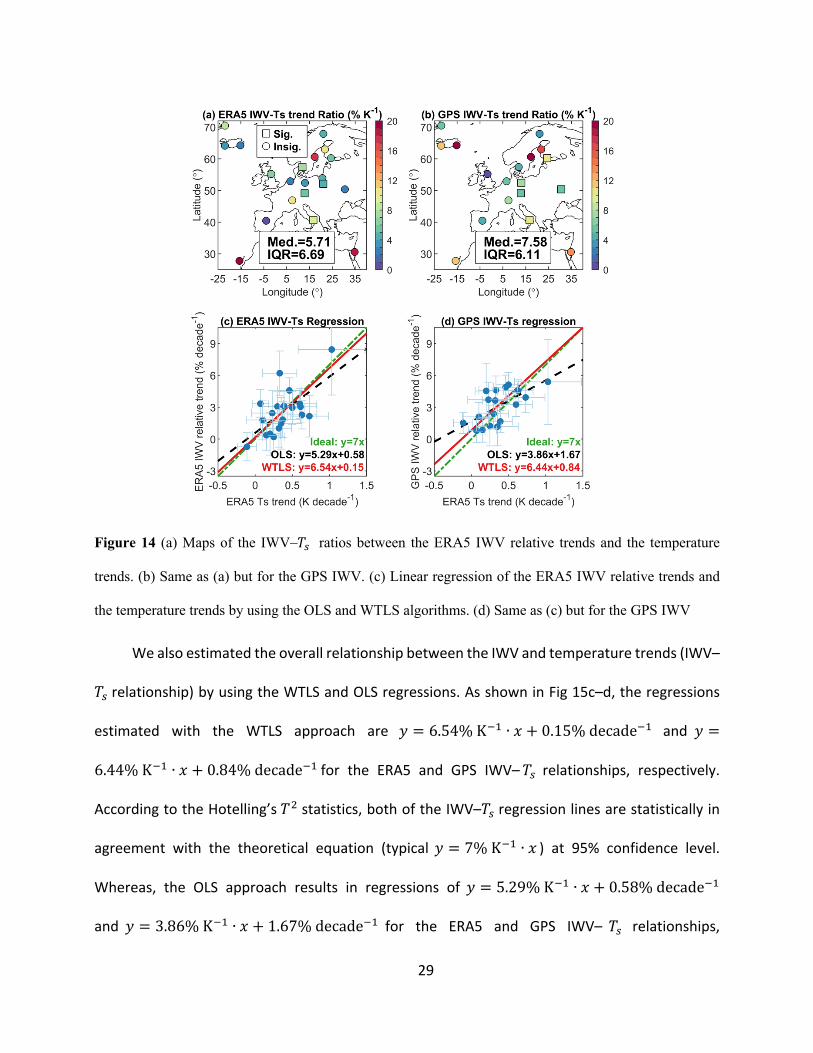
examine whether they are consistent with the theoretical prediction. Fig. 14a–14b show that the

trend ratios between IWV temperature are generally 0–20% K-1 for both the ERA5 and GPS IWV

with median values of 5.71% K-1 and 7.58% K-1, respectively. Moreover, both the ERA5 and GPS

ratios are generally larger in coastal areas (usually 7–15% K-1) than the European inland (usually

3–7% K-1).

29

Figure 14 (a) Maps of the IWV–𝑇! ratios between the ERA5 IWV relative trends and the temperature

trends. (b) Same as (a) but for the GPS IWV. (c) Linear regression of the ERA5 IWV relative trends and

the temperature trends by using the OLS and WTLS algorithms. (d) Same as (c) but for the GPS IWV

We also estimated the overall relationship between the IWV and temperature trends (IWV–

𝑇! relationship) by using the WTLS and OLS regressions. As shown in Fig 15c–d, the regressions

estimated with the WTLS approach are 𝑦 = 6.54%K4< ∙ 𝑥 + 0.15%decade4< and 𝑦 =

6.44%K4< ∙ 𝑥 + 0.84%decade4< for the ERA5 and GPS IWV–𝑇! relationships, respectively.

According to the Hotelling’s 𝑇1 statistics, both of the IWV–𝑇! regression lines are statistically in

agreement with the theoretical equation (typical 𝑦 = 7%K4< ∙ 𝑥 ) at 95% confidence level.

Whereas, the OLS approach results in regressions of 𝑦 = 5.29%K4< ∙ 𝑥 + 0.58%decade4<

and 𝑦 = 3.86%K4< ∙ 𝑥 + 1.67%decade4< for the ERA5 and GPS IWV– 𝑇! relationships,

30

respectively. Moreover, the last equation obtained with the OLS approach is significantly different

from the ideal prediction.

4 Discussion

4.1 Noise analysis

The statistical significance of the IWV trends is essential to a correct interpretation of

climate change but it is quite sensitive to the stochastic properties of the IWV series. Therefore,

a proper noise model should be selected. In this work, we found that the ARMA(1,1) model

outperforms many commonly used models, such as WN, WN+PL, AR(1), WN+AR(1), and

WN+ARMA(1,1) for the hourly ERA5 and GPS IWV series. This might be due to the fact that the

ARMA(1,1) model successfully fits the variations of the IWV spectra at various frequencies. In

particular, , the ARMA(1,1) model is capable to capture various characteristics of the spectra at

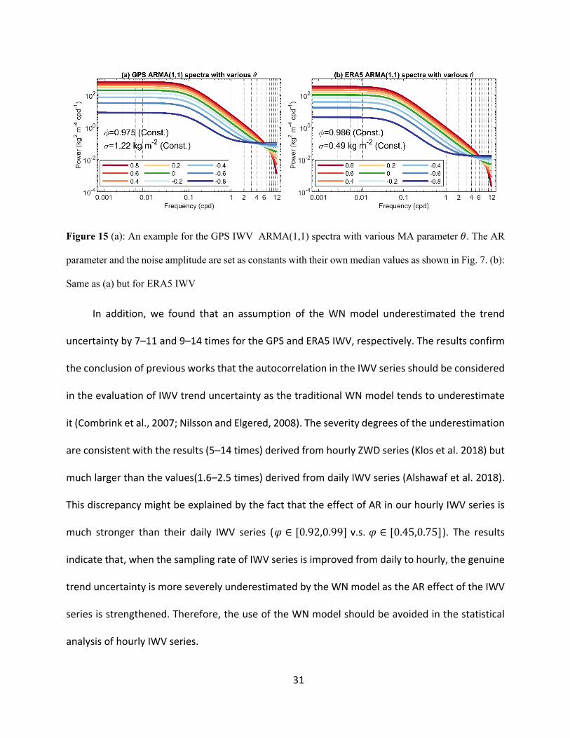
high frequencies (> 1cpd) by including the MA process. To illustrate this capability, Fig. 15

compares the spectra of various MA parameter when the AR parameter and the noise amplitude

are set as constants by using their own median values. Fig. 15 shows that the steep spectra curve

at the high frequencies flattens gradually when the MA parameter decreases from 0.8 to -0.8.

Therefore, the flat spectra curve of the GPS IWV series at high-frequency domain (Fig. 3 and

Fig. 5) can be modelled with negative MA parameters, whereas the steep spectra curve of the

ERA5 IWV series at that domain can be captured by positive MA parameters. This speculation is

confirmed by the noise analysis results as shown in Fig. 7. In sum, the ARMA(1,1) model is

recommended for the statistical analysis of hourly IWV series.

31

Figure 15 (a): An example for the GPS IWV ARMA(1,1) spectra with various MA parameter 𝜃. The AR

parameter and the noise amplitude are set as constants with their own median values as shown in Fig. 7. (b):

Same as (a) but for ERA5 IWV

In addition, we found that an assumption of the WN model underestimated the trend

uncertainty by 7–11 and 9–14 times for the GPS and ERA5 IWV, respectively. The results confirm

the conclusion of previous works that the autocorrelation in the IWV series should be considered

in the evaluation of IWV trend uncertainty as the traditional WN model tends to underestimate

it (Combrink et al., 2007; Nilsson and Elgered, 2008). The severity degrees of the underestimation

are consistent with the results (5–14 times) derived from hourly ZWD series (Klos et al. 2018) but

much larger than the values(1.6–2.5 times) derived from daily IWV series (Alshawaf et al. 2018).

This discrepancy might be explained by the fact that the effect of AR in our hourly IWV series is

much stronger than their daily IWV series (𝜑 ∈ [0.92,0.99] v.s. 𝜑 ∈ [0.45,0.75]). The results

indicate that, when the sampling rate of IWV series is improved from daily to hourly, the genuine

trend uncertainty is more severely underestimated by the WN model as the AR effect of the IWV

series is strengthened. Therefore, the use of the WN model should be avoided in the statistical

analysis of hourly IWV series.

32

4.2 Impacts of offsets and gaps

Many previous studies determined the offsets in the time series by using a significance test

with an assumption of WN model for simplicity (e.g., Klos et al., 2018), though Ning et al. (2016)

employed the AR(1) model. In this work, we found that the assumption of WN severely

underestimated the uncertainties of offsets (5–10 times) in addition to IWV trends. This result

indicates that a significance test with the WN model tends to erroneously accept unsignificant

offsets due to the unrealistically small offset uncertainties. Moreover, we found that the offsets

incorrectly validated by the WN model biased the IWV trend (relative changes from -246% to

196%) and amplified the trend uncertainties (up to 3 times) even though the ARMA(1,1) model

was used in the formal trend estimation. Therefore, we suggest that the ARMA(1,1) model should

be employed not only in the estimation of trends but also in the determination of offsets.

In addition to the offsets, gaps in GPS IWV series may also bias the trend estimation. In this

work, we found that the linear interpolation algorithm embedded in the Hector software works

quite well with the hourly IWV series. The algorithm introduced negligible trend bias even when

30% of data were randomly missing. However, the algorithm may bias the trend estimation by

more than 50% for more realistic cases with prolonged gaps in addition to the random ones. Thus,

we suggested that the IWV series with too long gaps should be excluded from trend analysis.

Likewise, Alshawaf et al. (2018) suggested that the gaps should not be longer than 1.5 years.

Future research should assess the effectiveness of more gap filling approaches, such as the

singular spectrum analysis used in Wang et al. (2016). Then, more well-founded rules on IWV

series selection can be made to avoid the artificial trends due to gaps.

33

4.3 Consistency between ERA5 and GPS IWV

In this study, we found that the ERA5 and GPS IWV time series agree quite well in Europe

though they suffer from representativeness differences. The biases are within ±1 kg m-2, the STD

of the differences are 0.9–2.6 kg m-2, and the correlation coefficients are larger than 0.92. The

results are consistent with previous works which compared the daily GPS IWV with ERA in Europe

(Alshawaf et al., 2018) and global (Bock and Parracho, 2019). However, the ERA5 is better than

the ERAI as the consistency between the hourly GPS and ERAI IWV series is likely to be worse than

the daily comparison due to interpolation (from daily/6-hourly to 1-hourly). Therefore, the ERA5

IWV is more preferred then ERAI.

As for the ERA5 and GPS IWV trends, most of them range from -0.1 to 0.8 kg m-2 decade-1,

which are consistent with previous works in Finland and Sweden (Nilsson and Elgered, 2008) and

in Europe (Alshawaf et al., 2018). However, the GPS IWV trends at stations JOZE and LAMA were

identified as outliers by using the IQR rule, as their values are too large (1.15 and 1.62 kg m-2

decade-1, respectively) with respect to their ERA5 IWV trends (0.48 and 0.27 kg m-2 decade-1,

respectively). As a comparison, Parracho et al. (2018) reported their IWV trends derived from

ERAI (0.51 and 0.19 kg m-2 decade-1) and from GPS (0.57 and 0.55 kg m-2 decade-1), which are

consistent with the ERA5 trends obtained in this work. The results suggest that the large ERA5–

GPS IWV trend discrepancy at these two stations might be due to GPS errors. It is unclear why the

GPS IWV trends are so large at these two stations. Nevertheless, we can exclude the possibility of

errors due to offsets for station JOZE, as its antenna stayed unchanged during the whole study

period. We will investigate the reason for the discrepancy in the further when more validation

information can be obtained.

34

Therefore, we used the rest 18 GPS IWV series to validate the suitability of using ERA5 IWV

in climate change. We estimated the trends of the IWV difference (dIWV = IWV]^_` − IWV*+,)

series as suggested by Wigley et al. (2006), to avoid the variance amplification effect (𝜎-.//0&')-1 =

𝜎]^_`0&')-1 + 𝜎*+,0&')-1) of the commonly used trend differences(𝑡𝑟𝑒𝑛𝑑"#$$ = 𝑡𝑟𝑒𝑛𝑑]^_`−𝑡𝑟𝑒𝑛𝑑*+,).

Results show that the dIWV trends are within ±0.4 kg m-2 decade-1, which agree with those values

between ERAI and GPS reported by Parracho et al. (2018). Moreover, the dIWV trends are

significant at 16 out of the 18 stations, though the ERA5 and GPS IWV trends are significant at 6

and 8 stations, respectively. As a comparison, we also calculated the trend differences, but none

of them is significant. The results suggest that the approach of estimating the trend of the

differential IWV series outperforms the approach of calculating the IWV trend difference, and

therefore it is recommended for the site-to-site comparison of IWV trends.

4.4 Water vapor feedback effect

Trenberth et al. (2003) implied that IWV increases 7% with 1 K growth of temperature if the

RH remains constant. However, Wang et al. (2016) argued that the RH changes with temperature

in the lower troposphere and thus alter the IWV–𝑇! trend ratio. If the RH increases with

temperature, the ratio will be above 7%, whereas if the RH decreases with temperature, the ratio

will be below 7%. In this work, we found that both the ERA5 and GPS IWV–𝑇! ratios are lower in

the European inland (usually 4–7% K-1) than in the coastal areas (usually 7–20% K-1). This could be

due to the fact that RH might be reduced by warming land surface as the land surface

evapotranspiration fail to satisfy the amount of moisture to keep RH constant (Wang et al., 2016).

35

Future studies should validate the speculation by investigating the local effects. Moreover, the

median ERA5 and GPS IWV–𝑇! trend ratios are 5.71% K-1 and 7.58% K-1, respectively. The values

are in accordance with previous works. For example, Chen and Liu (2016) reported that the

average IWV–𝑇! trend ratios over the world lands estimated with ERAI, NCEP-NCAR, Radiosonde,

and GPS are 6.4% K-1, 8.4% K-1, 5.3% K-1, and 5.6% K-1, respectively. A similar work also shows that

the GPS IWV–𝑇! trend ratios are 3–8 % K-1 in Europe (Alshawaf et al., 2018).

4.5 WTLS regression for the overall water vapor trend consistency and feedback effect

Linear regression has been widely used in the evaluation of IWV trend consistency (e.g. Ning et

al., 2016) and the feedback effect (e.g. Chen and Liu, 2016) as it can demonstrate more general

relationships than the comparison at each station. However, few studies have considered the

statistical significance of the IWV and 𝑇! trends. To overcome this deficiency, we proposed to use

the WTLS approach to calculate the regression line with the consideration of the deviations and

uncertainties of both dependent and independent variables. We found that, the regression

between the ERA5 and GPS IWV trends calculated with WTLS is 𝑦 = 0.93 ∙ 𝑥 +

0.10kgm41decade4< , which is statistically comparable to the ideal case of 𝑦 = 𝑥 at 95%

confidence level. Whereas, the OLS regression line is 𝑦 = 0.34 ∙ 𝑥 + 0.29kgm41decade4<, and

it was incorrectly identified as statistically different from the ideal case. Regarding the water

vapor feedback effect, we found that the WTLS regression equations are 𝑦 = 6.54%K4< ∙ 𝑥 +

0.15%decade4< and 𝑦 = 6.44%K4< ∙ 𝑥 + 0.84%decade4< for the ERA5 and GPS IWV– 𝑇!

relationships, respectively. Moreover, both are statistically in agreement with the theoretical

prediction (𝑦 = 7%K4< ∙ 𝑥) at 95% confidence level. However, the OLS regression equations for

36

them are = 5.29%K4< ∙ 𝑥 + 0.58%decade4< and 𝑦 = 3.86%K4< ∙ 𝑥 + 1.67%decade4< ,

respectively. Significance test shows that OLS regression of the GPS IWV–𝑇! relationship was

incorrectly identified as statistically different from the theoretical prediction. Therefore, we

suggest that the WTLS approach should also be used in the regression analysis of IWV trend

consistency and the water vapor feedback effect to avoid misinterpretation of climate change.

Moreover, the WTLS approach has an important advantage that it accepts the unsignificant IWV

trends, as many IWV trends are still unsignificant due to the deficiency of observing time period.

Furthermore, the WTLS regression can also be used with other IWV data sources, such as Very

Long Baseline Interferometry (VLBI, Steigenberger et al., 2007), satellite (Schröder et al., 2016),

radiosonde (Rinke et al., 2019) and so on.

5 Conclusions

In this study, the feasibility of the IWV derived from the state-of-the-art ERA5 for climate

change in Europe has been validated by GPS with the consideration of statistical significance. To

achieve reliable IWV trends with realistic trend uncertainty for the validation, we used

homogeneously reprocessed multidecadal (12–22 years) GPS IWV time series, proposed a data

screening approach with a robust moving median filter, selected the optimal noise model,

investigated the influences of GPS offsets determination and data gap filling on trend estimation.

Then, we introduced two approaches to evaluate the site-to-site and the overall IWV trend

consistency, respectively. For the site-to-site consistency, we estimated the trend of IWV

difference time series with realistic uncertainty instead of calculating the IWV trend difference

with amplified variance. Whereas for the overall consistency, we employed a linear regression

37

with WTLS approach with the consideration of deviations and uncertainties of both independent

and dependent variables. At last, the WTLS regression was also utilized to assess the water vapor

feedback effect. The main findings are as follows.

The ARMA(1,1) model outperforms many commonly used models, such as WN, WN+PL,

AR(1), WN+AR(1), and WN+ARMA(1,1) for the multidecadal hourly GPS and ERA5 IWV series, as

it successfully fits the variations of the IWV spectra at various frequencies. Therefore, the

ARMA(1,1) model is recommended for the statistical analysis of hourly IWV series. An improper

assumption of the noise model may result in unrealistic IWV trend uncertainty, for example, using

the WN model underestimates the trend uncertainty by 7–11 and 9–14 times for the GPS and

ERA5 IWV, respectively.

In addition, the assumption of WN severely underestimated the uncertainties of offsets (5–

10 times). Hence, a significance test with an assumption of WN tends to erroneously accept

unsignificant offsets due to the unrealistically small offset uncertainties. For the GPS IWV series

examined in this paper, this error in offsets validation biases the IWV trend (relative changes from

-246% to 196%) and amplifies the trend uncertainties (up to 3 times), even though the ARMA(1,1)

model is used in the formal trend estimation. Therefore, we suggest that the ARMA(1,1) model

should be used in GPS IWV offsets validation as well as trend estimation.

The linear interpolation algorithm introduced negligible trend bias even when 30% data

points of the hourly IWV time series are randomly missing. However, the algorithm may bias the

trend estimation by more than 50% for more realistic cases with prolonged gaps in addition to

the random ones. Thus, we suggest that the IWV series with too long gaps should be excluded

38

from trend analysis. Further works are certainly required to examine the effectiveness of more

gap filling approaches and to make more specific rules on IWV series selection.

When the ERA5 and GPS IWV trends are compared by calculating their differences, none of

the trend differences is significant due to the variance amplification effect. Nevertheless, with the

approach to estimate the trend of IWV difference time series, 89% of them are significant.

Therefore, the later approach is recommended for the comparison of IWV trends at station level.

The WTLS regression, which considers the deviations and uncertainties of both independent and

dependent variables, shows that the fitting line of ERA5 and GPS IWV trends is 𝑦 = 0.93 ∙ 𝑥 +

0.10kgm41decade4<. This regression line is statistically in agreement with the ideal case of 𝑦 =

𝑥 at 95% confidence level. Whereas the commonly used OLS regression incorrectly results in a

regression which is statistically different from the ideal case. Regarding the water vapor feedback

effect, the WTLS regression equations are 𝑦 = 6.54%K4< ∙ 𝑥 + 0.15%decade4< and 𝑦 =

6.44%K4< ∙ 𝑥 + 0.84%decade4< for the ERA5 and GPS IWV–𝑇! relationships, respectively. Both

statistically agree with the theoretical prediction (𝑦 = 7%K4< ∙ 𝑥). However, the OLS regression

makes a mistake again by obtaining the GPS IWV–𝑇! relationship which is statistically different

from the theoretical prediction. Therefore, the WTLS approach is suggested to be used in the

regression analysis of IWV trend consistency and the water vapor feedback effect to avoid

misinterpretations of climate change. The WTLS regression considers the uncertainty of all

variables, and thus it is capable to use the unsignificant IWV trends properly. This is a great

advantage in practice as many IWV trends are still unsignificant. Moreover, the WTLS regression

can also be used with other IWV data sources, such as VLBI, satellite, radiosonde and so on. For

the previous studies carried out with the OLS approach, if they are revisited with the

39

comprehensive WTLS approach, their regression results will be more proper, and the related

interpretations might be modified.

Acknowledgements

This work is performed under the German Research Foundation (DFG, project number:

321886779). Addisu Hunegnaw is funded through the Fonds National de la Recherche

Luxembourg Project VAPOUR (FNR Ref 12909050). The authors thank the European Centre for

Medium-Range Weather Forecasts for providing the ERA5 data sets.

References

[1] Alshawaf, F., Zus, F., Balidakis, K., Deng, Z., Hoseini, M., Dick, G. and Wickert, J.: On the statistical significance of climatic trends estimated from GPS tropospheric time series, Journal of Geophysical Research: Atmospheres, 123(19), 10–967, doi:10.1029/2018JD028703, 2018.

[2] Bevis, M. and Brown, A.: Trajectory models and reference frames for crustal motion geodesy, J Geod, 88(3), 283–311, doi:10.1007/s00190-013-0685-5, 2014.

[3] Bevis, M., Businger, S., Chiswell, S., Herring, T. A., Anthes, R. A., Rocken, C. and Ware, R. H.: GPS Meteorology: Mapping Zenith Wet Delays onto Precipitable Water, J. Appl. Meteor., 33(3), 379–386, doi:10.1175/1520-0450(1994)033<0379:GMMZWD>2.0.CO;2, 1994.

[4] Bevis, M., Businger, S., Herring, T. A., Rocken, C., Anthes, R. A. and Ware, R. H.: GPS meteorology: Remote sensing of atmospheric water vapor using the global positioning system, Journal of Geophysical Research: Atmospheres, 97(D14), 15787–15801, doi:10.1029/92JD01517, 1992.

[5] Bock, O. and Parracho, A. C.: Consistency and representativeness of integrated water vapour from ground-based GPS observations and ERA-Interim reanalysis, Atmospheric Chemistry and Physics, 19(14), 9453–9468, doi:10.5194/acp-19-9453-2019, 2019.

[6] Boehm, J., Werl, B. and Schuh, H.: Troposphere mapping functions for GPS and very long baseline interferometry from European Centre for Medium-Range Weather Forecasts operational analysis data, J. Geophys. Res., 111(B2), B02406, doi:10.1029/2005JB003629, 2006.

[7] Bos, M., Fernandes, R. and Bastos, L.: Hector user manual version 1.7. 2., 2019.

40

[8] Combrink, A. Z. A., Bos, M. S., Fernandes, R. M. S., Combrinck, W. L. and Merry, C. L.: On the importance of proper noise modelling for long-term precipitable water vapour trend estimations, South African Journal of Geology, 110(2–3), 211–218, doi:10.2113/gssajg.110.2-3.211, 2007.

[9] Dach, R., Lutz, S., Walser, P. and Fridez, P.: Bernese GNSS software version 5.2, University of Bern, Bern Open Publishing., 2015.

[10] Dai, A., Wang, J., Thorne, P. W., Parker, D. E., Haimberger, L. and Wang, X. L.: A New Approach to Homogenize Daily Radiosonde Humidity Data, J. Climate, 24(4), 965–991, doi:10.1175/2010JCLI3816.1, 2011.

[11] Davis, J. L., Herring, T. A., Shapiro, I. I., Rogers, A. E. E. and Elgered, G.: Geodesy by radio interferometry: Effects of atmospheric modeling errors on estimates of baseline length, Radio Science, 20(6), 1593–1607, doi:10.1029/RS020i006p01593, 1985.

[12] Held, I. M. and Soden, B. J.: Water Vapor Feedback and Global Warming, Annual Review of Energy and the Environment, 25(1), 441–475, doi:10.1146/annurev.energy.25.1.441, 2000.

[13] Hunegnaw, A., Teferle, F. N., Bingley, R. M. and Hansen, D. N.: Status of TIGA Activities at the British Isles Continuous GNSS Facility and the University of Luxembourg, in IAG 150 Years, edited by C. Rizos and P. Willis, pp. 617–623, Springer International Publishing, Cham., doi:10.1007/1345_2015_77, 2016.

[14] Jade, S. and Vijayan, M. S. M.: GPS-based atmospheric precipitable water vapor estimation using meteorological parameters interpolated from NCEP global reanalysis data, Journal of Geophysical Research: Atmospheres, 113(D3), doi:10.1029/2007JD008758, 2008.

[15] Klos, A., Hunegnaw, A., Teferle, F. N., Abraha, K. E., Ahmed, F. and Bogusz, J.: Noise characteristics in Zenith Total Delay from homogeneously reprocessed GPS time series, Atmospheric Measurement Techniques Discussions, 1–28, doi:10.5194/amt-2016-385, 2016.

[16] Krystek, M. and Anton, M.: A weighted total least-squares algorithm for fitting a straight line, Meas. Sci. Technol., 18(11), 3438–3442, doi:10.1088/0957-0233/18/11/025, 2007.

[17] Lacis, A. A., Schmidt, G. A., Rind, D. and Ruedy, R. A.: Atmospheric CO2: Principal Control Knob Governing Earth’s Temperature, Science, 330(6002), 356–359, doi:10.1126/science.1190653, 2010.

[18] Langbein, J.: Estimating rate uncertainty with maximum likelihood: differences between power-law and flicker–random-walk models, J Geod, 86(9), 775–783, doi:10.1007/s00190-012-0556-5, 2012.

[19] Malderen, R. V., Pottiaux, E., Klos, A., Domonkos, P., Elias, M., Ning, T., Bock, O., Guijarro, J., Alshawaf, F., Hoseini, M., Quarello, A., Lebarbier, E., Chimani, B., Tornatore, V., Kazancı, S. Z. and Bogusz, J.: Homogenizing GPS Integrated Water Vapor Time Series: Benchmarking Break Detection Methods on Synthetic Data Sets, Earth and Space Science, 7(5), e2020EA001121, doi:10.1029/2020EA001121, 2020.

[20] Mieruch, S., Noël, S., Bovensmann, H. and Burrows, J. P.: Analysis of global water vapour trends from satellite measurements in the visible spectral range, Atmospheric Chemistry and Physics, 8(3), 491–504, doi:10.5194/acp-8-491-2008, 2008.

[21] Myhre, G., Shindell, D., Bréon, F., Collins, W., Fuglestvedt, J., Huang, J., Koch, D., Lamarque, J., Lee, D., Mendoza, B. and others: Climate change 2013: the physical science basis, Contribution of working group I to the fifth assessment report of the intergovernmental panel on climate change, 659–740, 2013.

41

[22] Nilsson, T. and Elgered, G.: Long-term trends in the atmospheric water vapor content estimated from ground-based GPS data, Journal of Geophysical Research: Atmospheres, 113(D19), doi:10.1029/2008JD010110, 2008.

[23] Ning, T., Wickert, J., Deng, Z., Heise, S., Dick, G., Vey, S. and Schöne, T.: Homogenized Time Series of the Atmospheric Water Vapor Content Obtained from the GNSS Reprocessed Data, Journal of Climate, 29(7), 2443–2456, doi:10.1175/JCLI-D-15-0158.1, 2016.

[24] O’Gorman, P. A. and Muller, C. J.: How closely do changes in surface and column water vapor follow Clausius–Clapeyron scaling in climate change simulations, Environ. Res. Lett., 5(2), 025207, doi:10.1088/1748-9326/5/2/025207, 2010.

[25] Oladipo, E. O.: Spectral analysis of climatological time series: On the performance of periodogram, non-integer and maximum entropy methods, Theor Appl Climatol, 39(1), 40–53, doi:10.1007/BF00867656, 1988.

[26] Parracho, A. C., Bock, O. and Bastin, S.: Global IWV trends and variability in atmospheric reanalyses and GPS observations, Atmospheric Chemistry and Physics, 18(22), 16213–16237, doi:10.5194/acp-18-16213-2018, 2018.

[27] Petit, G. and Luzum, B.: IERS conventions (2010), No. IERS-TN-36. BUREAU INTERNATIONAL DES POIDS ET MESURES SEVRES (FRANCE)., 2010.

[28] Saastamoinen, J.: Atmospheric correction for the troposphere and stratosphere in radio ranging satellites, The use of artificial satellites for geodesy, 15, 247–251, doi:10.1029/GM015p0247, 1972.

[29] Schröder, M., Lockhoff, M., Forsythe, J. M., Cronk, H. Q., Vonder Haar, T. H. and Bennartz, R.: The GEWEX Water Vapor Assessment: Results from Intercomparison, Trend, and Homogeneity Analysis of Total Column Water Vapor, J. Appl. Meteor. Climatol., 55(7), 1633–1649, doi:10.1175/JAMC-D-15-0304.1, 2016.

[30] Simmons, A. J. and Gibson, J.: The ERA-40 project plan, European Centre for Medium-Range Weather Forecasts., 2000.

[31] Thorne, P. W. and Vose, R. S.: Reanalyses Suitable for Characterizing Long-Term Trends, Bull. Amer. Meteor. Soc., 91(3), 353–362, doi:10.1175/2009BAMS2858.1, 2010.

[32] Tiao, G. C., Reinsel, G. C., Xu, D., Pedrick, J. H., Zhu, X., Miller, A. J., DeLuisi, J. J., Mateer, C. L. and Wuebbles, D. J.: Effects of autocorrelation and temporal sampling schemes on estimates of trend and spatial correlation, Journal of Geophysical Research: Atmospheres, 95(D12), 20507–20517, doi:10.1029/JD095iD12p20507, 1990.

[33] Trenberth, K. E., Dai, A., Rasmussen, R. M. and Parsons, D. B.: The Changing Character of Precipitation, Bull. Amer. Meteor. Soc., 84(9), 1205–1218, doi:10.1175/BAMS-84-9-1205, 2003.

[34] Trenberth, K. E., Fasullo, J. T. and Mackaro, J.: Atmospheric Moisture Transports from Ocean to Land and Global Energy Flows in Reanalyses, J. Climate, 24(18), 4907–4924, doi:10.1175/2011JCLI4171.1, 2011.

[35] Vey, S., Dietrich, R., Fritsche, M., Rülke, A., Steigenberger, P. and Rothacher, M.: On the homogeneity and interpretation of precipitable water time series derived from global GPS observations, Journal of Geophysical Research: Atmospheres, 114(D10), doi:10.1029/2008JD010415, 2009.

[36] Wang, J., Dai, A. and Mears, C.: Global Water Vapor Trend from 1988 to 2011 and Its Diurnal Asymmetry Based on GPS, Radiosonde, and Microwave Satellite Measurements, J. Climate, 29(14), 5205–5222, doi:10.1175/JCLI-D-15-0485.1, 2016.

42

[37] Wang, J., Zhang, L. and Dai, A.: Global estimates of water-vapor-weighted mean temperature of the atmosphere for GPS applications, Journal of Geophysical Research: Atmospheres, 110(D21), doi:10.1029/2005JD006215, 2005.

[38] Wang, X. L.: Accounting for Autocorrelation in Detecting Mean Shifts in Climate Data Series Using the Penalized Maximal t or F Test, J. Appl. Meteor. Climatol., 47(9), 2423–2444, doi:10.1175/2008JAMC1741.1, 2008.

[39] Wang, X., Zhang, K., Wu, S., Fan, S. and Cheng, Y.: Water vapor-weighted mean temperature and its impact on the determination of precipitable water vapor and its linear trend, Journal of Geophysical Research: Atmospheres, 121(2), 833–852, doi:10.1002/2015JD024181, 2018.

[40] Wang, Z., Zhou, X., Xing, Z., Tang, Q., Ma, D. and Ding, C.: Comparison of GPS-based precipitable water vapor using various reanalysis datasets for the coastal regions of China, Theor Appl Climatol, 137(1), 1541–1553, doi:10.1007/s00704-018-2687-y, 2019.

[41] Wigley, T., Santer, B. and Lanzante, J.: Temperature Trends in the Lower Atmosphere; Appendix A: Statistical Issues Regarding Trends., 2006.

[42] Williams, S. D. P.: The effect of coloured noise on the uncertainties of rates estimated from geodetic time series, Journal of Geodesy, 76(9–10), 483–494, doi:10.1007/s00190-002-0283-4, 2003.

[43] Yuan, P., Jiang, W., Wang, K., Sneeuw, N., Yuan, P., Jiang, W., Wang, K. and Sneeuw, N.: Effects of Spatiotemporal Filtering on the Periodic Signals and Noise in the GPS Position Time Series of the Crustal Movement Observation Network of China, Remote Sensing, 10(9), 1472, doi:10.3390/rs10091472, 2018.

[44] Steigenberger, P., Tesmer, V., Krügel, M., Thaller, D., Schmid, R., Vey, S. and Rothacher, M.: Comparisons of homogeneously reprocessed GPS and VLBI long time-series of troposphere zenith delays and gradients, J Geod, 81(6), 503–514, doi:10.1007/s00190-006-0124-y, 2007.

[45] Rinke, A., Segger, B., Crewell, S., Maturilli, M., Naakka, T., Nygård, T., Vihma, T., Alshawaf, F., Dick, G., Wickert, J. and Keller, J.: Trends of Vertically Integrated Water Vapor over the Arctic during 1979–2016: Consistent Moistening All Over?, J. Climate, 32(18), 6097–6116, doi:10.1175/JCLI-D-19-0092.1, 2019.

43

Table S1 Trends of ERA5 and GPS IWV time series and their difference (dIWV=ERA5-GPS) time series

estimated with the ARMA(1,1) model. Unit: kg m-2 decade-1

Station Latitude

(°) Longitude

(°) Height

(m) ERA5 GPS dIWV

Trend STD Trend STD Trend STD

GLSV 50.36 30.50 200.8 0.33 0.30 0.60 0.22 -0.23 0.02

HOFN 64.27 344.80 17.3 0.06 0.24 0.54 0.31 0.12 0.03

JOZE 52.10 21.03 109.9 0.48 0.24 1.15 0.19 -0.60 0.03

KIR0 67.88 21.06 469.2 0.14 0.23 0.11 0.17 0.05 0.01

LAMA 53.89 20.67 157.6 0.27 0.25 1.62 0.37 -1.39 0.03

MAR6 60.60 17.26 50.5 0.24 0.25 0.28 0.18 -0.06 0.01

MAS1 27.76 344.37 153.6 0.63 0.25 0.15 0.21 0.24 0.04

MATE 40.65 16.70 490.2 0.73 0.19 0.78 0.18 -0.04 0.03

METS 60.22 24.40 75.8 0.38 0.20 0.66 0.15 -0.35 0.02

MORP 55.21 358.31 94.4 -0.11 0.20 0.23 0.15 -0.14 0.02

ONSA 57.40 11.93 9.0 0.45 0.20 0.24 0.15 0.16 0.01

POTS 52.38 13.07 104.0 0.36 0.21 0.72 0.16 -0.41 0.01

RAMO 30.60 34.76 868.2 0.70 0.24 0.52 0.15 0.08 0.03

REYK 64.14 338.04 26.6 0.12 0.21 0.43 0.14 -0.24 0.02

SCOR 70.49 338.05 71.5 0.61 0.31 0.39 0.29 0.26 0.04

VAAS 62.96 21.77 40.1 0.31 0.27 0.47 0.21 -0.31 0.02

VILL 40.44 356.05 595.4 0.03 0.22 0.19 0.29 0.34 0.04

WSRT 52.91 6.60 40.5 0.06 0.24 0.14 0.19 -0.07 0.01

WTZR 49.14 12.88 619.2 0.47 0.20 0.46 0.16 -0.10 0.01

ZIMM 46.88 7.47 906.7 0.40 0.18 0.31 0.18 0.02 0.02

Table S2 Significant offsets of the GPS IWV time series validated with the ARMA(1,1) model. Unit: mm

Station Epoch (modified Julian date) Offset STD

HOFN 52173.75 -1.54 0.32

HOFN 53241.00 -1.38 0.34

LAMA 54421.79 -1.68 0.42

MATE 51347.00 -1.10 0.28

VILL 53276.50 -0.85 0.37

ZIMM 51123.00 -0.72 0.31