Embed Size (px)
Citation preview

Feasibility Analysis of Trajectory Planning Problems of Automated Vehicles in Time-Varying Environments
Sebastian Söntges
10.2.2017

Motivation - Trajectory planning for automated vehicles
• Find a collision-free trajectory from a starting state to a goal region
2

Motivation - Trajectory planning for automated vehicles
• Find a collision-free trajectory from a starting state to a goal region
2

Motivation - Trajectory planning for automated vehicles
• Find a collision-free trajectory from a starting state to a goal region
2
Goal regions

Motivation - Trajectory planning for automated vehicles
• Find a collision-free trajectory from a starting state to a goal region
2
Goal regions
?
?

Feasibility
• Commonly used sampling-based approach:
• Our set-based approach:
3
Can prove feasibility, but cannot detect infeasibility.
Cannot detect feasibility, but can prove infeasibility.
time: 1.50 sec of 3.00 sec

Definition - Trajectory planning problem
Given:• A dynamic system of the car• constraint dynamics• a set of (time-varying) obstacles• occupied region of the vehicle • initial state at time • goal region at time
4
x(t) = f(x(t),u(t))
O(t) ⇢ R2
A(x(t)) ⇢ R2
x0
XGtf
t0
Find collision-free ( , ) trajectory
connecting start and goal.
u(t) 2 U(x(t))
A(x(t)) \O(t) = ; t 2 [t0, tf ]
x(t) = x0 +
Z t
t0
f(x(t0),u(t0)) dt0

Definition - Anticipated reachable set
• Reachable set: Set of all states which can be reached by a dynamic system
• We extend this definition through two restrictions:1. Each state is reachable by a collision-free trajectory2. Each state can be continued by a collision-free
trajectory until the end of the planning horizon
5
t1
t1
t2
t2 t
f
t1 t2 t
f
Fig. 1. Reachable set considering collision free trajectories until the giventime step (top); anticipated reachable set considering only collision freetrajectories for the whole planning horizon [t0, t
f
] (bottom).
4) an initial state x0 at time t0,5) and a goal region X
G
at time t
f
.A solution of the trajectory planning problem is an inputsignal u(t), such that the corresponding trajectory
⌧(t;u,x0) := x0 +
Z
t
t0
f(x(t
0),u(t
0))dt
0 (1)
connects the initial state ⌧(t0;u,x0) = x0 to a state in thegoal region ⌧(t
f
;u,x0) 2 XG
and does not collide with anyobstacle A(x(t
0)) \O(t
0) = ;, 8t0 2 [t0, tf ].
The states attained by the set of all trajectories at sometime t are related to the reachable set of the dynamicalsystem.
Definition 2 (Anticipated reachable set): The reachableset is defined as the set of all states which can be reachedby the system from a given initial set X0 at a given timet. We extend the common definition of the reachable setto the anticipated reachable set through two restrictions.First, we only consider states that can be reached at time t
without any collision with the obstacle set O(t). Second, werequire that the state can be continued by a collision-freetrajectory until the end of the planning horizon t
f
. Tosimplify the notation, we introduce the set of forbiddenstates F(t) := {x(t)|A(x(t)) \O(t) 6= ;}. Thus,
reach(X0, t, tf ) :=
n
⌧(t;u,x0)
�
�
�
9u 2 ˜U , 9x0 2 X0,
⌧(t
0;u,x0)) /2 F(t
0) for t0 2 [t0, tf ]
o
,
(2)where ˜U is the set of all possible input signals.
Fig. 1 shows the motivation behind this definition. For agiven scenario, the ego vehicle must merge either into theleft or right lane in order to avoid a collision. If the vehiclemerges into the left lane, it can reach some region in theleft lane for several time steps. However, it will eventuallycollide with some obstacle within the planning horizon t
f
.Planning trajectories in these regions must be avoided. Theanticipated reachable set excludes these regions.
Often, not the full state x(t), but only the position of thevehicle (x(t), y(t))
T is of interest.
Definition 3 (Projection): Given the state x(t) in statespace X , the projection
proj
xy
(x(t)) := (x(t), y(t))
T (3)
is defined as the mapping from the state to the position ofthe vehicle.
We use the same notation to project a set of states X 0 ✓ X :
proj
xy
(X 0) := {proj
xy
(x)|x 2 X 0}. (4)A frequent decision for a driver is to choose between
passing an obstacle on the left or right. In order to groupfeasible trajectories into different high-level decisions, acommon method is to apply topological concepts of pathhomotopy and homology to motion planning [11]. Two pathswith the same starting point and the same endpoint are said tobe homotopic, iff there exists a continuous mapping, whichdeforms one path to the other. In particular this means thatthe path must not “jump” over any obstacle.
Fig. 2 shows an example of the ego vehicle and twomoving vehicles in the spatial-time domain. Vehicle A drivesin the same lane as the ego vehicle. Vehicle B drives inthe opposite lane and passes both other vehicles. Threepossible trajectories ⌧1,2,3 of the ego vehicle are shown.This example is a modified version of the one presentedin [5] with the difference that we assume that there is freespace between vehicle A and B when both pass each other.In this example, ⌧2 and ⌧3 first pass vehicle B and thenovertake vehicle A. However, since both do not share thesame endpoint, they are not homotopic. In contrast, ⌧1 and⌧3 are homotopic since they share both the same startingpoint and endpoint and can continuously be deformed toeach other (under the assumption that vehicle A and B do nottouch and the ego vehicle can drive between both). However,this grouping seems counterintuitive. It seems more naturalto group trajectories ⌧2 and ⌧3 as the maneuver “first passvehicle B, then overtake vehicle A”. In this work, we proposea method for grouping trajectories which is inspired by amethod for identifying homotopy between paths using two-dimensional sub-manifolds in the three dimensional position-time domain of the vehicle [14]. However, in contrast to[14], our goal is not to group paths into homotopy classes inits strict mathematical definition due to the aforementionedproblems, but to find a grouping which fits the semanticmeaning in terms of automated driving (e.g. passing anothervehicle on the left).
The idea is to construct for each trajectory a “word” whichdescribes the trajectory and assigns it to a unique drivingcorridor. All trajectories with the same word belong to thesame driving corridor.
Definition 4 (Word construction): Given a set of two-dimensional oriented surfaces U
i
in the three-dimensionalspatial-time domain with an associated “letter” r
i
and atrajectory ⌧ . We assign a word to ⌧ by concatenating theletters in the order of all intersections of ⌧ with U
i
. If Ui
iscrossed in the direction of its orientation we use the letter r
i
and if it is crossed opposing its orientation, we use the inverseletter r
�1i
. If a letter r
i
and its inverse r
�1i
follow directly

Definition - Anticipated reachable set
• Definition of the “anticipated reachable set“:
• with the set of colliding states
• : trajectory for initial state and input signal
• : set of input signals, : set of initial states
6
F(t) := {x(t)|A(x(t)) \O(t) 6= ;}
reachant(t) :=n
⌧(t;u,x0)
�
�
�
9u 2 ˜U , 9x0 2 X0,
⌧(t0;u,x0)) /2 F(t0) for t0 2 [t0, tf ]o
⌧(t;u,x0) x0 u
X0U

Feasibility of trajectory planning problem (1)
• A trajectory planning problem is feasible, iff
• For systems with constraint dynamics and time-varying obstacles, common trajectory planners only discover a subset:
• In general, cannot be computed efficiently.
7
reachant(tf ) \ XG 6= ;.
reachant(t)
reachs(t) ⇢ reachant(t)

Feasibility of trajectory planning problem (2)
• Since common trajectory planner can prove that a problem is feasible,
but they cannot detect infeasible problems.
• An over-approximation can prove that a problem is infeasible,
8
reachs(t) ⇢ reachant(t)
reachc(t) � reachant(t)
reachc(tf ) \ XG = ; ) reachant(tf ) \ XG = ;.
reachs(tf ) \ XG 6= ; ) reachant(tf ) \ XG 6= ;

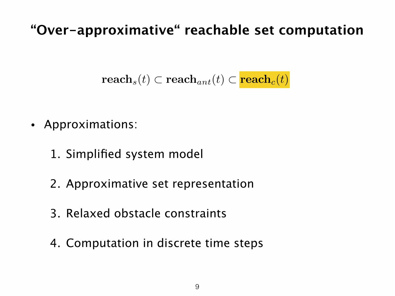
“Over-approximative“ reachable set computation
• Approximations:
1. Simplified system model
2. Approximative set representation
3. Relaxed obstacle constraints
4. Computation in discrete time steps
9
reachs(t) ⇢ reachant(t) ⇢ reachc(t)
“Over-approximative“ reachable set computation
• Approximations:
1. Simplified system model
2. Approximative set representation
3. Relaxed obstacle constraints
4. Computation in discrete time steps
9
reachs(t) ⇢ reachant(t) ⇢ reachc(t)

Simplified system model
• Double integrator in x- and y-direction
• Bounded speed and acceleration
• Abstraction of any realistic vehicle
10
f(x,u) =
0
BB@
x
x
y
y
1
CCA =
0
BB@
0 1 0 00 0 0 00 0 0 10 0 0 0
1
CCA
0
BB@
x
x
y
y
1
CCA+
0
BB@
0 01 00 00 1
1
CCA
✓u
x
u
y
◆
|ux
| a
max,x
|uy
| a
max,y
v
min,x
x v
max,x
v
min,y
y v
max,y

Approximative set representation
• Set representation:
with convex polytopes
and for .
• The convex polytopes allow for an efficient computation of linear system dynamics
• The decomposition of allows to consider obstacles
11
P (q)i,x/y
reachc(t)
int(B(l)i ) \ int(B(r)
i ) = ; r 6= l
reachc
(ti
) =[
q
B(q)i
=[
q
P(q)i,x
⇥ P(q)i,y

• Dynamics decoupled along x- and y-direction
• Coupling through collision avoidance constraints
Reachable set of acceleration bounded double integrator (1)
12
f(x,u) =
0
BB@
x
x
y
y
1
CCA =
0
BB@
0 1 0 00 0 0 00 0 0 10 0 0 0
1
CCA
0
BB@
x
x
y
y
1
CCA+
0
BB@
0 01 00 00 1
1
CCA
✓u
x
u
y
◆
|ux
| a
max,x
|uy
| a
max,y
v
min,x
x v
max,x
v
min,y
y v
max,y

Reachable set of acceleration bounded double integrator (2)
13
✓x
x
◆=
✓0 10 0
◆
| {z }A
✓x
x
◆+
✓01
◆
|{z}B
u
x
|ux
| a
max,x
reach(t) =⇢s
����9s0 2 X0, 9u 2 U , s = eAts0 +
Zt
0eA(t�⌧)Bu(⌧)d⌧
�
= eAtX0 �⇢s
����9u 2 U , s =
Zt
0eA(t�⌧)Bu(⌧)d⌧
�
| {z }=:P
u,x
(t)
= eAtX0 � Pu,x
(t)

Reachable set of acceleration bounded double integrator (2)
13
✓x
x
◆=
✓0 10 0
◆
| {z }A
✓x
x
◆+
✓01
◆
|{z}B
u
x
|ux
| a
max,x
reach(t) =⇢s
����9s0 2 X0, 9u 2 U , s = eAts0 +
Zt
0eA(t�⌧)Bu(⌧)d⌧
�
= eAtX0 �⇢s
����9u 2 U , s =
Zt
0eA(t�⌧)Bu(⌧)d⌧
�
| {z }=:P
u,x
(t)
= eAtX0 � Pu,x
(t)
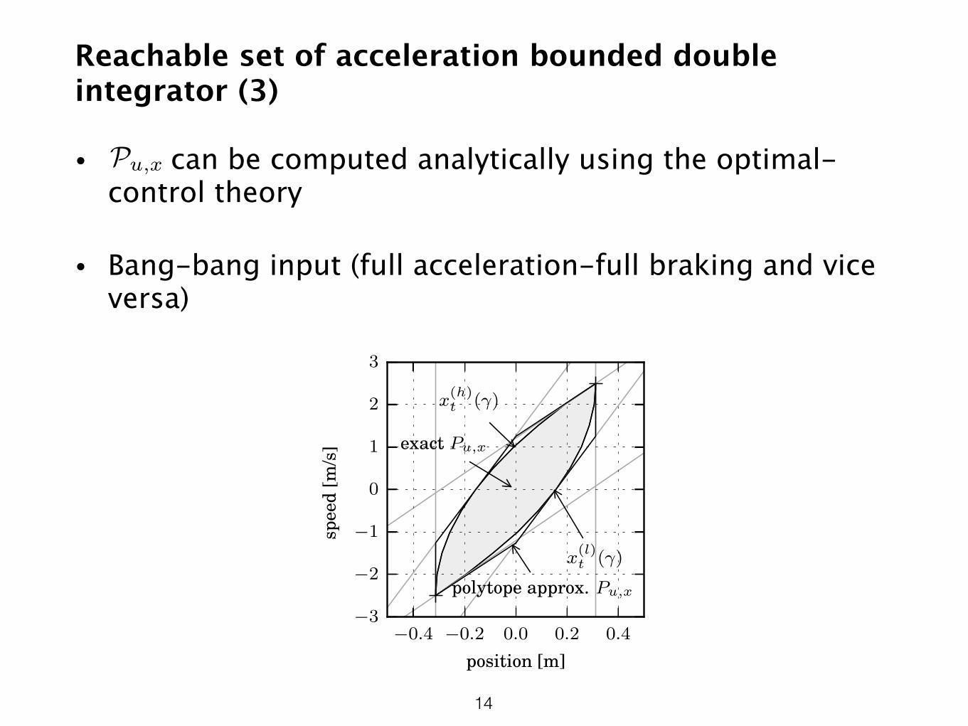
Reachable set of acceleration bounded double integrator (3)
• can be computed analytically using the optimal-control theory
• Bang-bang input (full acceleration-full braking and vice versa)
14
−0.4 −0.2 0.0 0.2 0.4
position [m]
−3
−2
−1
0
1
2
3
spee
d[m
/s]
x(h)t (γ)
x(l)t (γ)
exact Pu,x
polytope approx. Pu,x
Pu,x

Algorithm - Forward propagation
15
propagate
x
(P(q)i�1,x) :=
✓⇢✓1 �t
0 1
◆s
���� s 2 P(q)i�1,x
�� P
u,x
(�t)
◆
\⇢✓x
x
◆���� vmin,x
x v
max,x
�
1
Algorithm 1
Input: initial set X0 = [q
B
(q)0 ;
Output: {B(q)i
}q
for i = 1, . . . , n1: for i = 1 to n do2: for all B(q)
i�1 in time step i� 1 do3: P(q)
i�1,x = propagate
x
(P(q)i�1,x)
4: P(q)i�1,y = propagate
y
(P(q)i�1,y)
5: B(q)i�1 = (P(q)
i�1,x ⇥ P(q)i�1,y)
6: end for7: {B(r)
i
}r
= overapproximate([B(q)i�1) \ F(t
i
))8: end for
P(q)i�1,x :=
✓⇢✓1 �t
0 1
◆s
���� s 2 P(q)i�1,x
�� P
u,x
(�t)
◆
\⇢✓x
x
◆���� vmin,x
x v
max,x
�
propagate
x
(P(q)i�1,x) (1)

Over-approximate (1)
16
[B(q)i�1 \ F(ti)
[
r
B(r)i = overapproximate([ ˆB(q)
i�1 \ F(ti))

Over-approximate (1)
16
may overlap arbitrary shape[
r
B(r)i
= P(r)i,x
⇥ P(r)i,y
int(B(l)i ) \ int(B(r)
i ) = ;
P(r)i,x/y
with convex polytopes
[B(q)i�1 \ F(ti)
[
r
B(r)i = overapproximate([ ˆB(q)
i�1 \ F(ti))

Over-approximate (2)
• Project 4-dimensional set into 2-dimensional position domain
• Merge and partition projected set into axis-aligned boxes
• Split boxes until collision free
• Create from each box a 4-dimensional
17
F(ti)
projxy(B(q)i−1)
ti−1
projxy(B(q)i−1)
propagated
Rect(q)
discretized
Poly(m)
merged
Rect(p)
partitioned
Rect(s)
collision detection and split
B(r)i
[B(q)i�1 \ F(ti)

Over-approximate (3)
• Each new is created from and as follows:
• and similarly for .
18
B(r)i
P(r)
i,x
=Convhull
0
@[
q2parent(s)
⇣ˆP(q)
i�1,x
\⇢✓x
x
◆����Box
(r)
min,x
x Box
(r)
max,x
�◆!
P(r)i,x
P(r)i,y
P(r)i,y
[B(q)i�1 \ F(ti)

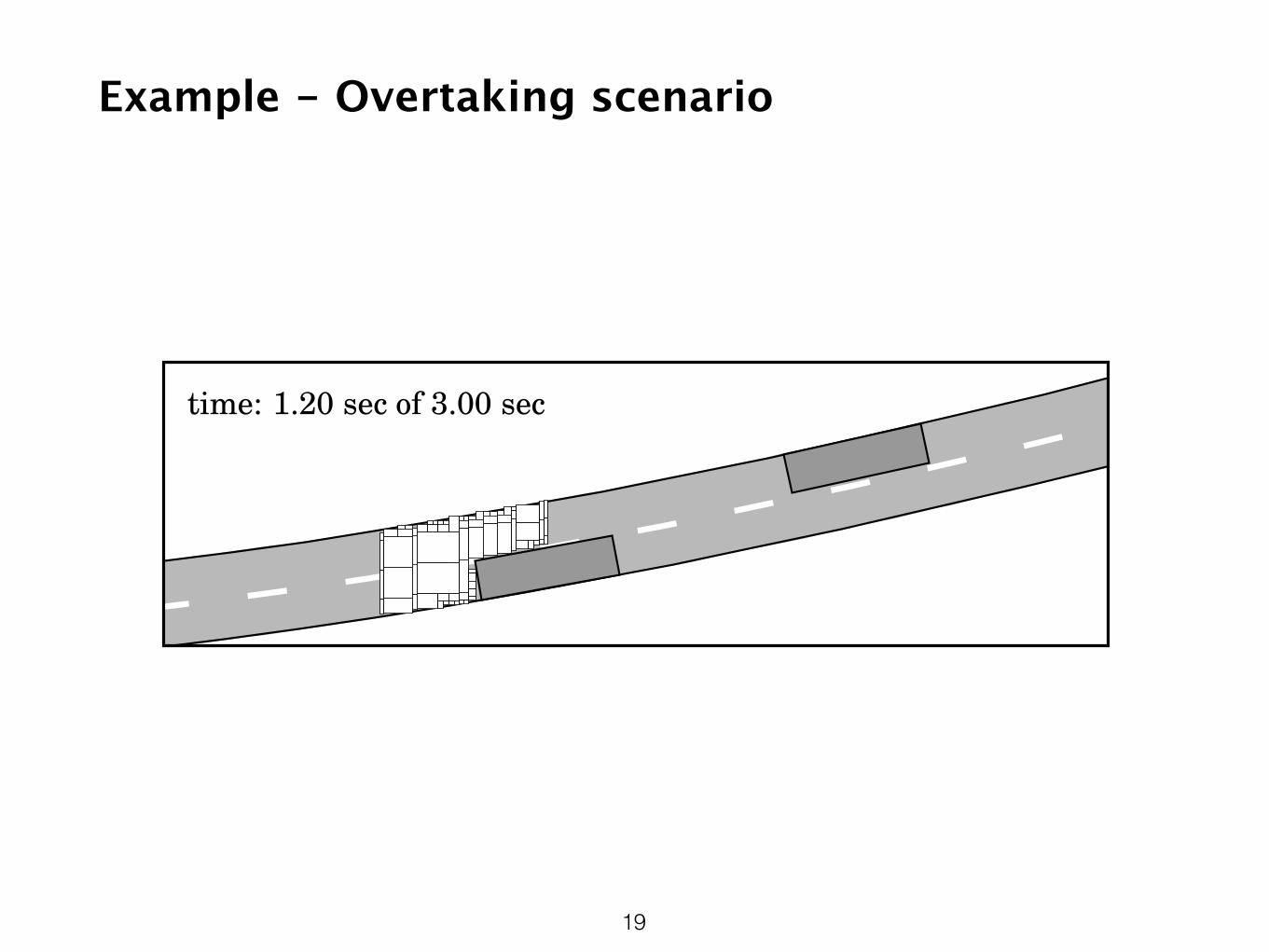
Example - Overtaking scenario
19
car B
car Aego carinitial scenario

Example - Overtaking scenario
19
car B
car Aego carinitial scenariotime: 0.00 sec of 3.00 sec

Example - Overtaking scenario
19
car B
car Aego carinitial scenariotime: 0.00 sec of 3.00 sectime: 0.00 sec of 3.00 sec

Example - Overtaking scenario
19
car B
car Aego carinitial scenariotime: 0.00 sec of 3.00 sectime: 0.00 sec of 3.00 sectime: 0.15 sec of 3.00 sec

Example - Overtaking scenario
19
car B
car Aego carinitial scenariotime: 0.00 sec of 3.00 sectime: 0.00 sec of 3.00 sectime: 0.15 sec of 3.00 sectime: 0.30 sec of 3.00 sec

Example - Overtaking scenario
19
car B
car Aego carinitial scenariotime: 0.00 sec of 3.00 sectime: 0.00 sec of 3.00 sectime: 0.15 sec of 3.00 sectime: 0.30 sec of 3.00 sectime: 0.45 sec of 3.00 sec

Example - Overtaking scenario
19
car B
car Aego carinitial scenariotime: 0.00 sec of 3.00 sectime: 0.00 sec of 3.00 sectime: 0.15 sec of 3.00 sectime: 0.30 sec of 3.00 sectime: 0.45 sec of 3.00 sectime: 0.60 sec of 3.00 sec

Example - Overtaking scenario
19
car B
car Aego carinitial scenariotime: 0.00 sec of 3.00 sectime: 0.00 sec of 3.00 sectime: 0.15 sec of 3.00 sectime: 0.30 sec of 3.00 sectime: 0.45 sec of 3.00 sectime: 0.60 sec of 3.00 sectime: 0.75 sec of 3.00 sec

Example - Overtaking scenario
19
car B
car Aego carinitial scenariotime: 0.00 sec of 3.00 sectime: 0.00 sec of 3.00 sectime: 0.15 sec of 3.00 sectime: 0.30 sec of 3.00 sectime: 0.45 sec of 3.00 sectime: 0.60 sec of 3.00 sectime: 0.75 sec of 3.00 sectime: 0.90 sec of 3.00 sec

Example - Overtaking scenario
19
car B
car Aego carinitial scenariotime: 0.00 sec of 3.00 sectime: 0.00 sec of 3.00 sectime: 0.15 sec of 3.00 sectime: 0.30 sec of 3.00 sectime: 0.45 sec of 3.00 sectime: 0.60 sec of 3.00 sectime: 0.75 sec of 3.00 sectime: 0.90 sec of 3.00 sectime: 1.05 sec of 3.00 sec
Example - Overtaking scenario
19
car B
car Aego carinitial scenariotime: 0.00 sec of 3.00 sectime: 0.00 sec of 3.00 sectime: 0.15 sec of 3.00 sectime: 0.30 sec of 3.00 sectime: 0.45 sec of 3.00 sectime: 0.60 sec of 3.00 sectime: 0.75 sec of 3.00 sectime: 0.90 sec of 3.00 sectime: 1.05 sec of 3.00 sectime: 1.20 sec of 3.00 sec

Example - Overtaking scenario
19
car B
car Aego carinitial scenariotime: 0.00 sec of 3.00 sectime: 0.00 sec of 3.00 sectime: 0.15 sec of 3.00 sectime: 0.30 sec of 3.00 sectime: 0.45 sec of 3.00 sectime: 0.60 sec of 3.00 sectime: 0.75 sec of 3.00 sectime: 0.90 sec of 3.00 sectime: 1.05 sec of 3.00 sectime: 1.20 sec of 3.00 sectime: 1.35 sec of 3.00 sec

Example - Overtaking scenario
19
car B
car Aego carinitial scenariotime: 0.00 sec of 3.00 sectime: 0.00 sec of 3.00 sectime: 0.15 sec of 3.00 sectime: 0.30 sec of 3.00 sectime: 0.45 sec of 3.00 sectime: 0.60 sec of 3.00 sectime: 0.75 sec of 3.00 sectime: 0.90 sec of 3.00 sectime: 1.05 sec of 3.00 sectime: 1.20 sec of 3.00 sectime: 1.35 sec of 3.00 sectime: 1.50 sec of 3.00 sec

Example - Overtaking scenario
19
car B
car Aego carinitial scenariotime: 0.00 sec of 3.00 sectime: 0.00 sec of 3.00 sectime: 0.15 sec of 3.00 sectime: 0.30 sec of 3.00 sectime: 0.45 sec of 3.00 sectime: 0.60 sec of 3.00 sectime: 0.75 sec of 3.00 sectime: 0.90 sec of 3.00 sectime: 1.05 sec of 3.00 sectime: 1.20 sec of 3.00 sectime: 1.35 sec of 3.00 sectime: 1.50 sec of 3.00 sectime: 1.65 sec of 3.00 sec

Example - Overtaking scenario
19
car B
car Aego carinitial scenariotime: 0.00 sec of 3.00 sectime: 0.00 sec of 3.00 sectime: 0.15 sec of 3.00 sectime: 0.30 sec of 3.00 sectime: 0.45 sec of 3.00 sectime: 0.60 sec of 3.00 sectime: 0.75 sec of 3.00 sectime: 0.90 sec of 3.00 sectime: 1.05 sec of 3.00 sectime: 1.20 sec of 3.00 sectime: 1.35 sec of 3.00 sectime: 1.50 sec of 3.00 sectime: 1.65 sec of 3.00 sectime: 1.80 sec of 3.00 sec

Example - Overtaking scenario
19
car B
car Aego carinitial scenariotime: 0.00 sec of 3.00 sectime: 0.00 sec of 3.00 sectime: 0.15 sec of 3.00 sectime: 0.30 sec of 3.00 sectime: 0.45 sec of 3.00 sectime: 0.60 sec of 3.00 sectime: 0.75 sec of 3.00 sectime: 0.90 sec of 3.00 sectime: 1.05 sec of 3.00 sectime: 1.20 sec of 3.00 sectime: 1.35 sec of 3.00 sectime: 1.50 sec of 3.00 sectime: 1.65 sec of 3.00 sectime: 1.80 sec of 3.00 sectime: 1.95 sec of 3.00 sec

Example - Overtaking scenario
19
car B
car Aego carinitial scenariotime: 0.00 sec of 3.00 sectime: 0.00 sec of 3.00 sectime: 0.15 sec of 3.00 sectime: 0.30 sec of 3.00 sectime: 0.45 sec of 3.00 sectime: 0.60 sec of 3.00 sectime: 0.75 sec of 3.00 sectime: 0.90 sec of 3.00 sectime: 1.05 sec of 3.00 sectime: 1.20 sec of 3.00 sectime: 1.35 sec of 3.00 sectime: 1.50 sec of 3.00 sectime: 1.65 sec of 3.00 sectime: 1.80 sec of 3.00 sectime: 1.95 sec of 3.00 sectime: 2.10 sec of 3.00 sec

Example - Overtaking scenario
19
car B
car Aego carinitial scenariotime: 0.00 sec of 3.00 sectime: 0.00 sec of 3.00 sectime: 0.15 sec of 3.00 sectime: 0.30 sec of 3.00 sectime: 0.45 sec of 3.00 sectime: 0.60 sec of 3.00 sectime: 0.75 sec of 3.00 sectime: 0.90 sec of 3.00 sectime: 1.05 sec of 3.00 sectime: 1.20 sec of 3.00 sectime: 1.35 sec of 3.00 sectime: 1.50 sec of 3.00 sectime: 1.65 sec of 3.00 sectime: 1.80 sec of 3.00 sectime: 1.95 sec of 3.00 sectime: 2.10 sec of 3.00 sectime: 2.25 sec of 3.00 sec

Example - Overtaking scenario
19
car B
car Aego carinitial scenariotime: 0.00 sec of 3.00 sectime: 0.00 sec of 3.00 sectime: 0.15 sec of 3.00 sectime: 0.30 sec of 3.00 sectime: 0.45 sec of 3.00 sectime: 0.60 sec of 3.00 sectime: 0.75 sec of 3.00 sectime: 0.90 sec of 3.00 sectime: 1.05 sec of 3.00 sectime: 1.20 sec of 3.00 sectime: 1.35 sec of 3.00 sectime: 1.50 sec of 3.00 sectime: 1.65 sec of 3.00 sectime: 1.80 sec of 3.00 sectime: 1.95 sec of 3.00 sectime: 2.10 sec of 3.00 sectime: 2.25 sec of 3.00 sectime: 2.40 sec of 3.00 sec

Example - Overtaking scenario
19
car B
car Aego carinitial scenariotime: 0.00 sec of 3.00 sectime: 0.00 sec of 3.00 sectime: 0.15 sec of 3.00 sectime: 0.30 sec of 3.00 sectime: 0.45 sec of 3.00 sectime: 0.60 sec of 3.00 sectime: 0.75 sec of 3.00 sectime: 0.90 sec of 3.00 sectime: 1.05 sec of 3.00 sectime: 1.20 sec of 3.00 sectime: 1.35 sec of 3.00 sectime: 1.50 sec of 3.00 sectime: 1.65 sec of 3.00 sectime: 1.80 sec of 3.00 sectime: 1.95 sec of 3.00 sectime: 2.10 sec of 3.00 sectime: 2.25 sec of 3.00 sectime: 2.40 sec of 3.00 sectime: 2.55 sec of 3.00 sec

Example - Overtaking scenario
19
car B
car Aego carinitial scenariotime: 0.00 sec of 3.00 sectime: 0.00 sec of 3.00 sectime: 0.15 sec of 3.00 sectime: 0.30 sec of 3.00 sectime: 0.45 sec of 3.00 sectime: 0.60 sec of 3.00 sectime: 0.75 sec of 3.00 sectime: 0.90 sec of 3.00 sectime: 1.05 sec of 3.00 sectime: 1.20 sec of 3.00 sectime: 1.35 sec of 3.00 sectime: 1.50 sec of 3.00 sectime: 1.65 sec of 3.00 sectime: 1.80 sec of 3.00 sectime: 1.95 sec of 3.00 sectime: 2.10 sec of 3.00 sectime: 2.25 sec of 3.00 sectime: 2.40 sec of 3.00 sectime: 2.55 sec of 3.00 sectime: 2.70 sec of 3.00 sec

Example - Overtaking scenario
19
car B
car Aego carinitial scenariotime: 0.00 sec of 3.00 sectime: 0.00 sec of 3.00 sectime: 0.15 sec of 3.00 sectime: 0.30 sec of 3.00 sectime: 0.45 sec of 3.00 sectime: 0.60 sec of 3.00 sectime: 0.75 sec of 3.00 sectime: 0.90 sec of 3.00 sectime: 1.05 sec of 3.00 sectime: 1.20 sec of 3.00 sectime: 1.35 sec of 3.00 sectime: 1.50 sec of 3.00 sectime: 1.65 sec of 3.00 sectime: 1.80 sec of 3.00 sectime: 1.95 sec of 3.00 sectime: 2.10 sec of 3.00 sectime: 2.25 sec of 3.00 sectime: 2.40 sec of 3.00 sectime: 2.55 sec of 3.00 sectime: 2.70 sec of 3.00 sectime: 2.85 sec of 3.00 sec

Example - Overtaking scenario
19
car B
car Aego carinitial scenariotime: 0.00 sec of 3.00 sectime: 0.00 sec of 3.00 sectime: 0.15 sec of 3.00 sectime: 0.30 sec of 3.00 sectime: 0.45 sec of 3.00 sectime: 0.60 sec of 3.00 sectime: 0.75 sec of 3.00 sectime: 0.90 sec of 3.00 sectime: 1.05 sec of 3.00 sectime: 1.20 sec of 3.00 sectime: 1.35 sec of 3.00 sectime: 1.50 sec of 3.00 sectime: 1.65 sec of 3.00 sectime: 1.80 sec of 3.00 sectime: 1.95 sec of 3.00 sectime: 2.10 sec of 3.00 sectime: 2.25 sec of 3.00 sectime: 2.40 sec of 3.00 sectime: 2.55 sec of 3.00 sectime: 2.70 sec of 3.00 sectime: 2.85 sec of 3.00 sectime: 3.00 sec of 3.00 sec
braking
overtaking

Example - Overtaking scenario
20
time: 1.50 sec of 3.00 sec
min. speed x-axis
xy
speed
max. speed y-axis
xy
speed
min. speed y-axis
xy
speed
max. speed x-axis
xy
speed

Example - Highway scenario
21
Sampling-based:
Set-based:

Improve reachable set approximation
Part 2

Improved approximation
• Up to now, only previous time steps are used to calculate the reachable set:
• Future collisions can be used to tighten the reachable set
23
reachs(t) ⇢ reachant(t) ⇢ reachc(t)
reachant(t) :=n
⌧(t;u,x0)
�
�
�
9u 2 ˜U , 9x0 2 X0,
⌧(t0;u,x0)) /2 F(t0) for t0 2 [t0, tf ]o

Improved approximation
• Up to now, only previous time steps are used to calculate the reachable set:
• Future collisions can be used to tighten the reachable set
23
reachs(t) ⇢ reachant(t) ⇢ reachc(t)
reachant(t) :=n
⌧(t;u,x0)
�
�
�
9u 2 ˜U , 9x0 2 X0,
⌧(t0;u,x0)) /2 F(t0) for t0 2 [t0, tf ]ot

Backward minimal reachable set
• Inevitable collision states
• Computation of the exact set of inevitable collision states needs again a reachability analysis
• Under-approximation
24

Backward minimal reachable set
• Inevitable collision states
• Computation of the exact set of inevitable collision states needs again a reachability analysis
• Under-approximation
24

Double integrator revised
• Additional constraints: must be in interval
25
✓x
x
◆=
✓0 10 0
◆
| {z }A
✓x
x
◆+
✓01
◆
|{z}B
u
x
|ux
| a
max,x
x(t1) 2 I1, x(t2) 2 I2, . . . , x(tn
) 2 I
n
x(ti) Ii

Double integrator revised
26
position [m]
02468
10
tim
est
ep
(a)
Position constraints
position [m]−15
−10
−5
0
5
10
15
spee
d[m
/s]
(b)
P1
Pn
Reachable states
−5 0 5
position [m]
−15
−10
−5
0
5
10
15
spee
d[m
/s]
(c)
P1
Pn
Reachable states using backward reach set

−10−5 0 5 10
position
−10
−5
0
5
10
spee
d
(a)
tj
−10−5 0 5 10
position
spee
d
(b)
ti
Double integrator revised
• If must be in , then must be in ( with ):
27
x(tj) Ij
ICS(Ij
, t
i
) =
⇢(x
i
, x
i
)T����
✓�1 ��t
ij
1 �t
ij
◆✓x
i
x
i
◆
✓�I
i,min,x
+ 12amax
�t
2ij
I
i,max,x
+ 12amax
�t
2ij
◆�
(x(ti), x(ti))T
�tij = tj � ti

Double integrator revised
28
position [m]
02468
10
tim
est
ep
(a)
Position constraints
position [m]−15
−10
−5
0
5
10
15
spee
d[m
/s]
(b)
P1
Pn
Reachable states
−5 0 5
position [m]
−15
−10
−5
0
5
10
15
spee
d[m
/s]
(c)
P1
Pn
Reachable states using backward reach set

Algorithm - Forward, backward propagation
29
propagate
x
(
ˆP(q)i�1,x) =
✓⇢✓1 �t
0 1
◆s
���s 2 P(q)i�1,x
�� P
u,x
(�t)
◆
\⇢✓x
x
◆|v
min,x
x v
max,x
�
\0
@n\
j=i
ICS(Ij,x
, t
i
)
1
A
1
Algorithm 1
Input: initial set X0 = [q
B
(q)0 ; forbidden set F(t); con-
straints I
i,x
, I
i,y
Output: {B(q)i
}q
for i = 1, . . . , n1: for i = 1 to n do2: for all B(q)
i�1 in time step i� 1 do3: P(q)
i�1,x = propagate
x
(P(q)i�1,x)
4: P(q)i�1,y = propagate
y
(P(q)i�1,y)
5: B(q)i�1 = (P(q)
i�1,x ⇥ P(q)i�1,y)
6: end for7: {B(r)
i
}r
= overapproximate([B(q))i�1) \ F(t
i
))8: end for
P(q)i�1,x :=
✓⇢✓1 �t
0 1
◆s
���� s 2 P(q)i�1,x
�� P
u,x
(�t)
◆
\⇢✓x
x
◆���� vmin,x
x v
max,x
�
propagate
x
(P(q)i�1,x) (1)

Construction of constraints
1. Run forward algorithm
2. Construct bounding boxes
3. Run forward, backward algorithm
30
RectCi constraints from first run
RectCnRectC0
second run
first run

Conclusion
• A method for computing an over-approximation of the reachable set for velocity and acceleration bounded systems in time-varying environments is proposed
• Infeasibility of trajectory planning problem can be proven
• The method is complementary to sampling-based methods in the sense, that an under- and over-approximation of the reachable set is computed
• It may be used to improve search heuristics of sampling-based methods
• Runtime <100ms makes it applicable to automated vehicles
31