Embed Size (px)
Citation preview
Fearing the Fed:
How Wall Street Reads Main Street
Tzuo-Hann Law
Boston College
Dongho Song
Boston College
Amir Yaron
University of Pennsylvania & NBER
This Version: September 18, 2017
Abstract
We provide strong evidence of persistent cyclical variation in the sensitivity of stock prices
to macroeconomic news announcement (MNA) surprises. Starting from a phase in which the
stock market is insensitive to news, it becomes increasingly sensitive as the economy enters
a recession with peak sensitivity obtained a year after the recession started. As the economy
expands, the sensitivity comes down to its starting point in four to five years. We then show
that market expectation about the future interest rate path is one of the primary drivers of
the cyclical variations in stock price responsiveness to news surprises. These new empirical
facts are robust to various measures of stock returns and MNA surprises. We introduce a
simple regime-switching dividend growth model in which beliefs over the duration of monetary
regimes drive the sensitivity of returns to news surprises. The model analysis illustrates that
the evolution of market expectations about monetary policy can generate the time-varying
return responses observed in the data.
Keywords: Macroeconomic news announcements, intraday stock return sensitivity, cyclical vari-
ation, monetary policy expectations.
JEL Classification: G12, E30, E40, E50.
We are grateful to Yakov Amihud, Susanto Basu, Jesus Fernandez-Villaverde, Peter Ireland, Sophia Li, EricSwanson, and Jonathan Wright for insightful comments that improved the paper significantly. We thank seminarparticipants at the BC-BU Green Line Macro Meeting, Metzler Bank, the Fall 2016 Midwest Macro Meeting, the2017 Midwest Finance Association Meeting, Federal Reserve Bank of New York, Federal Reserve Bank of Philadel-phia, Goethe Univesity, New York University, the 2017 Society for Economic Dynamics meeting, Tel-Aviv Univer-sity, and University of Pennsylvania. Correspondence: Department of Economics, Boston College, 140 Common-wealth Avenue, Chestnut Hill, MA 02467. Email: [email protected] (Tzuo-Hann Law) and [email protected](Dongho Song). The Wharton School, Finance Department, University of Pennsylvania, Philadelphia, PA 19104.Email: [email protected] (Amir Yaron).
1
1 Introduction
Recent evidence points to the prominent role the Federal Open Market Committee (FOMC)
meetings and other macroeconomic news announcements (MNA) have on financial markets (e.g.,
Lucca and Moench (2015) and Savor and Wilson (2013)). However, predicting the direction of
the stock market’s response to these news is challenging. For example, better-than-expected
MNA surprises that push prices up through higher expected future cash flows might instead be
offset via expected future interest rate hikes as a result of stabilization policy. The perception
about stabilization policy, in particular by the Federal Reserve (henceforth Fed), will depend
on the phase of the business cycle and economic conditions. Furthermore, market’s perception
could be asymmetric with respect to negative and positive MNA surprises (e.g., consider the
recent zero-lower bound (ZLB) period during which the Fed had limited control over negative
MNA surprises). This interaction between market conditions and perceptions about possible Fed
response can lead to significant time variation in the stock market’s reaction.1 Motivated by
these considerations, this paper examines the cyclical variations in the sensitivity of the stock
market to MNA surprises.
We use various measures of high-frequency stock returns and surveys of market expectations of
upcoming MNAs. Our benchmark sample spans early 2000 to late 2016. We estimate the time-
varying sensitivity of stock returns to the MNA surprises with the nonlinear regression method
used in Swanson and Williams (2014). We focus on the MNAs and not on the FOMC meetings as
the former allows us to include many more events over the business cycle and measure precisely
the impact of surprises on stock market.
First, contrary to the literature on the FOMC meetings, we show that unconditionally it
is difficult to detect a significant response of the stock market to the MNA surprises. Yet,
consistent with the motivation above, we establish that this muted unconditional response is
masking significant and time varying cyclical responses of stock prices to the MNA surprises. The
sensitivity of stock prices to the MNA surprises starts to increase entering a recession, continues
to increase as the recession deepens, and peaks post-recession. Peak sensitivity is about twice the
average sensitivity. The transition from peak sensitivity to trough sensitivity takes about four to
five years with the recovery taking about the same amount of time. At trough sensitivity, stock
prices generally do not react to the MNA surprises. We interpret these findings as reflecting the
overall informativeness of the announcements given economic conditions. The relatively muted
responses during early recession and late expansion periods are a result of the MNAs that are
1See McQueen and Roley (1993), Flannery and Protopapadakis (2002), Boyd, Hu, and Jagannathan (2005) andAndersen, Bollerslev, Diebold, and Vega (2007) for early explorations relating MNAs and stock market responses.
2
perceived as (i) carrying temporary shocks and/or (ii) ones for which (uncertainty about) the
Fed stabilization policy makes them effectively uninformative.
Second, and somewhat surprisingly, there is no evidence for asymmetry in the responses to
negative and positive MNA surprises. Third, the sensitivity of short-term interest rate futures
to the MNA surprises moves in lock-step but in the opposite direction as that of stock prices’.
We provide many robustness tests: the most important ones being that our results by and large
persist (i) when we measure the responses using daily returns and (ii) when we extend our analysis
to data beginning in 1990 which encompass three recessions.
To shed light on the mechanism at work, we use a novel state space approach to write the
stock return news as the sum of news about cash flows, news about the risk-free rate, and news
about risk premium following Campbell (1991). To isolate the role of risk premium news in stock
return variation, we use intraday variance premium as an empirical proxy for risk premium news.
Interestingly, we find that news concerning cash flows and the risk-free rate explain most of the
sensitivity pattern we observe in the data. This important effect of cashflows (and risk-free rate)
on stock prices is of interest given the long standing research in analyzing the sources of variation
of valuation ratios.
After narrowing down the informational content of the MNA surprises to news about cash flows
and/or news about risk-free rates, we propose a simple regime-switching dividend growth model
to further understand the role of beliefs about future dividend growth and interest rate path in
accounting for stock return variation. In our simple framework, the nominal short rate is the
monetary policy instrument and is thought to vary jointly with dividend growth. The regime-
switching model features two distinct economic regimes. In the “Reactive Monetary Policy
(R-MP)” regime, positive dividend growth shocks can increase both future dividend growth and
future interest rates. In this regime, high interest rates slow down future dividend growth. In the
“Non-Reactive Monetary Policy (NR-MP)” regime, dividend growth evolves in an autoregressive
pattern and the interest rate does not impact the dividend growth. The key feature in the
NR-MP regime is that dividend growth shock is entirely transmitted to future dividend growth
without a countervailing rise in the interest rate. Finally, we assume that the time varying
Markov transition probabilities govern transitions between the two states.
Given plausible VAR dynamics and Markov transition probabilities, this simple model yields
time-varying reaction of stock prices to shocks that are qualitatively similar to what is observed
in the data. We interpret these transition probabilities as reflecting beliefs about the duration of
the economic regimes at each point in time to help clarify the underlying response mechanism.
First, beliefs about the duration of the “R-MP” regime inversely track the time-varying sensitivity
coefficient for stock returns. This is intuitive because in the “R-MP” regime by construction the

3
interest rate diminishes the pure cash flow effects. In contrast, in the “NR-MP” regime, the
cash flow effects dominate if the beliefs that no interest rate change will take place persist (i.e.,
staying in the “NR-MP” regime). Second, under the extracted transition probabilities, we show
that the risks of an interest rate hike (transition from the “NR-MP” to the “R-MP” regime) could
entirely mitigate the positive cash flow shock. This model analysis illustrates that the evolution
of market beliefs about monetary policy can generate the time varying return response observed
in the data. We close our analysis by showing that such qualitative results can be reconciled in
a modern dynamic (consumption-based) asset pricing model that incorporates regime-switching
(aggressive and loose) monetary policy.
1.1 Literature Review
The literature has identified accommodating time variation and using high-frequency returns as
key steps in measuring the impact of MNA surprises on stock prices. McQueen and Roley (1993)
first demonstrate that the link between MNA surprises and stock prices is much stronger after
accounting for different stages of the business cycle. Boyd, Hu, and Jagannathan (2005) use
model-based forecasts of the unemployment rate and Andersen, Bollerslev, Diebold, and Vega
(2007) rely on survey forecasts to emphasize the importance of measuring the impact of MNA
surprises on stock prices over different phases of the business cycle. We add to this literature by
characterizing the time varying properties of the stock market’s reaction to MNA surprises and
its tight relationship with market expectations of monetary policy.
More generally, our paper can be linked to a large literature that studies asset market and
monetary policy, for example, Pearce and Roley (1985), Thorbecke (1997), Cochrane and Piazzesi
(2002), Rigobon and Sack (2003), Rigobon and Sack (2004), Bernanke and Kuttner (2005),
Gurkaynak, Rigobon, and Sack (2005), and Bekaert, Hoerova, and Lo Duca (2013) among others.
More recently, Neuhierl and Weber (2016) document that monetary policy affects stock prices
outside of the scheduled FOMC announcements as predicted by Bernanke and Kuttner (2005).
Cieslak and Vissing-Jorgensen (2017) focus on a related and complementary channel regarding
the relationship between stock market movements and subsequent monetary policy by the Fed.
The remainder of this paper is organized as follows. Section 2 describes the data, unconditional
results, regression methods, selection of macroeconomic announcements, and discusses empirical
findings. Section 3 decomposes the announcments into cashflow and risk premia components
and illustrates the key role beliefs regarding interest rate play in the return reponse. Section 4
illustrates the mechanism within a calibrated dynamic asset-pricing model. Section 5 provides
concluding remarks.
4
2 Empirical Analysis
2.1 High-Frequency Data
Macroeconomic News Announcements. MNAs are officially released by government bodies
and private institutions at regular prescheduled intervals. In this paper, we use the MNAs from
the Bureau of Labor Statistics (BLS), Bureau of the Census (BC), Bureau of Economic Anal-
ysis (BEA), Federal Reserve Board (FRB), Conference Board (CB), Employment and Training
Administration (ETA), and, Institute for Supply Management (ISM). We use the MNAs as tabu-
lated by Bloomberg Financial Services. Bloomberg also surveys professional economists on their
expectations of these macroeconomic announcements. Forecasters can submit or update their
predictions up to the night before the official release of the MNAs. Thus, Bloomberg forecasts
should in principle reflect all available information until the publication of the MNAs. Most
announcements are monthly except Initial Jobless Claims which is weekly. All announcements
are released at either 8:30am or 10:00am except Industrial Production MoM which is released
at 9:15am. Announcements released outside of their regular schedule are dropped. We consider
announcements where the data span January 2000 to December 2016. Details are provided in
Table B.1. For robustness, we also consider Money Market Services (MMS) real-time data on
expected U.S. macroeconomic fundamentals. None of our results are affected.
Standardization of the MNA Surprises. Denote MNA i at time t by MNAi,t and let
Et−∆(MNAi,t) be median surveyed forecast made at time t−∆. The individual MNA surprises
(after normalization) are collected in X whose ith component is
Xi,t =MNAi,t − Et−∆(MNAi,t)
Normalization.
The units of measurement differ across the macroeconomic indicators. To allow for meaning-
ful comparisons of the estimated surprise response coefficients, we consider two normalizations.
The first normalization scales the individual MNA surprise by the contemporaneous level of un-
certainty measured by the standard deviation of all survey forecasts. The key feature of this
standardization is that the normalization constant differs across time for each MNA surprise.
The second normalization scales each MNA surprise by its standard deviation taken over the
entire sample period. It includes future announcements that have yet to occur from the per-
spective of the economic agent.2 The key feature of the second approach is that for each MNA
surprise, the normalization constant is identical across time. Thus, this normalization cannot
affect the statistical significance of sensitivity coefficient. Surprisingly, as reported in Table B.2
2This standardization was proposed by Balduzzi, Elton, and Green (2001) and is widely used in the literature.
5
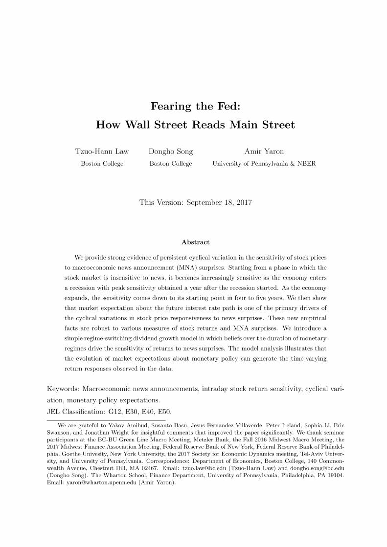
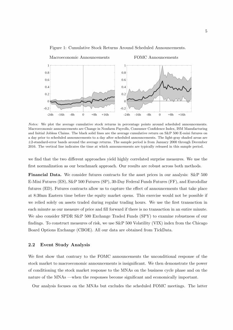
Figure 1: Cumulative Stock Returns Around Scheduled Announcements.
Macroeconomic Announcements FOMC Announcements
-24h -16h -8h 0 +8h +16h
-0.2
0
0.2
0.4
0.6
0.8
1
-24h -16h -8h 0 +8h +16h
-0.2
0
0.2
0.4
0.6
0.8
1
Notes: We plot the average cumulative stock returns in percentage points around scheduled announcements.
Macroeconomic announcements are Change in Nonfarm Payrolls, Consumer Confidence Index, ISM Manufacturing
and Initial Jobless Claims. The black solid lines are the average cumulative return on S&P 500 E-mini futures on
a day prior to scheduled announcements to a day after scheduled announcements. The light-gray shaded areas are
±2-standard-error bands around the average returns. The sample period is from January 2000 through December
2016. The vertical line indicates the time at which announcements are typically released in this sample period.
we find that the two different approaches yield highly correlated surprise measures. We use the
first normalization as our benchmark approach. Our results are robust across both methods.
Financial Data. We consider futures contracts for the asset prices in our analysis: S&P 500
E-Mini Futures (ES), S&P 500 Futures (SP), 30-Day Federal Funds Futures (FF), and Eurodollar
futures (ED). Futures contracts allow us to capture the effect of announcements that take place
at 8:30am Eastern time before the equity market opens. This exercise would not be possible if
we relied solely on assets traded during regular trading hours. We use the first transaction in
each minute as our measure of price and fill forward if there is no transaction in an entire minute.
We also consider SPDR S&P 500 Exchange Traded Funds (SPY) to examine robustness of our
findings. To construct measures of risk, we use S&P 500 Volatility (VIX) index from the Chicago
Board Options Exchange (CBOE). All our data are obtained from TickData.
2.2 Event Study Analysis
We first show that contrary to the FOMC announcements the unconditional response of the
stock market to macroeconomic announcements is insignificant. We then demonstrate the power
of conditioning the stock market response to the MNAs on the business cycle phase and on the
nature of the MNAs —when the responses become significant and economically important.
Our analysis focuses on the MNAs but excludes the scheduled FOMC meetings. The latter
6
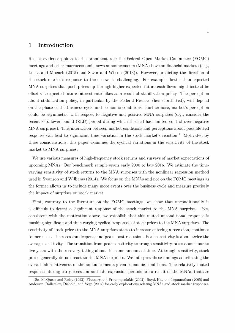
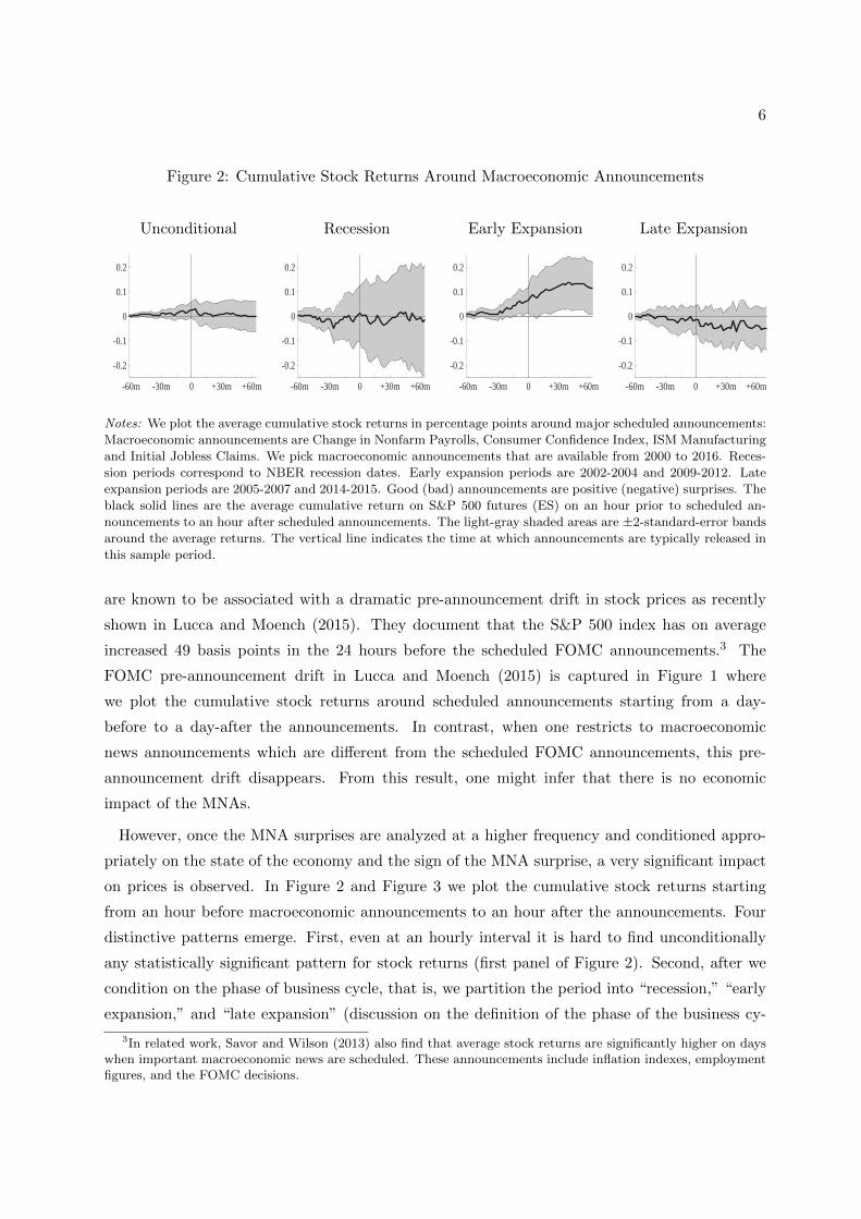
Figure 2: Cumulative Stock Returns Around Macroeconomic Announcements
Unconditional Recession Early Expansion Late Expansion
-60m -30m 0 +30m +60m
-0.2
-0.1
0
0.1
0.2
-60m -30m 0 +30m +60m
-0.2
-0.1
0
0.1
0.2
-60m -30m 0 +30m +60m
-0.2
-0.1
0
0.1
0.2
-60m -30m 0 +30m +60m
-0.2
-0.1
0
0.1
0.2
Notes: We plot the average cumulative stock returns in percentage points around major scheduled announcements:
Macroeconomic announcements are Change in Nonfarm Payrolls, Consumer Confidence Index, ISM Manufacturing
and Initial Jobless Claims. We pick macroeconomic announcements that are available from 2000 to 2016. Reces-
sion periods correspond to NBER recession dates. Early expansion periods are 2002-2004 and 2009-2012. Late
expansion periods are 2005-2007 and 2014-2015. Good (bad) announcements are positive (negative) surprises. The
black solid lines are the average cumulative return on S&P 500 futures (ES) on an hour prior to scheduled an-
nouncements to an hour after scheduled announcements. The light-gray shaded areas are ±2-standard-error bands
around the average returns. The vertical line indicates the time at which announcements are typically released in
this sample period.
are known to be associated with a dramatic pre-announcement drift in stock prices as recently
shown in Lucca and Moench (2015). They document that the S&P 500 index has on average
increased 49 basis points in the 24 hours before the scheduled FOMC announcements.3 The
FOMC pre-announcement drift in Lucca and Moench (2015) is captured in Figure 1 where
we plot the cumulative stock returns around scheduled announcements starting from a day-
before to a day-after the announcements. In contrast, when one restricts to macroeconomic
news announcements which are different from the scheduled FOMC announcements, this pre-
announcement drift disappears. From this result, one might infer that there is no economic
impact of the MNAs.
However, once the MNA surprises are analyzed at a higher frequency and conditioned appro-
priately on the state of the economy and the sign of the MNA surprise, a very significant impact
on prices is observed. In Figure 2 and Figure 3 we plot the cumulative stock returns starting
from an hour before macroeconomic announcements to an hour after the announcements. Four
distinctive patterns emerge. First, even at an hourly interval it is hard to find unconditionally
any statistically significant pattern for stock returns (first panel of Figure 2). Second, after we
condition on the phase of business cycle, that is, we partition the period into “recession,” “early
expansion,” and “late expansion” (discussion on the definition of the phase of the business cy-
3In related work, Savor and Wilson (2013) also find that average stock returns are significantly higher on dayswhen important macroeconomic news are scheduled. These announcements include inflation indexes, employmentfigures, and the FOMC decisions.
7
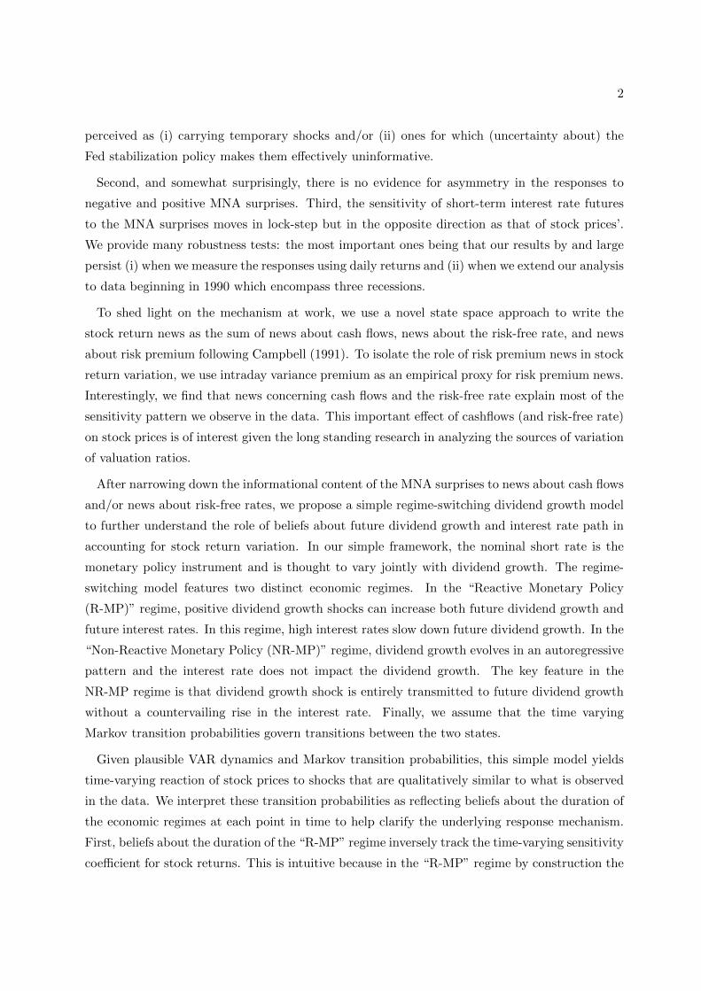
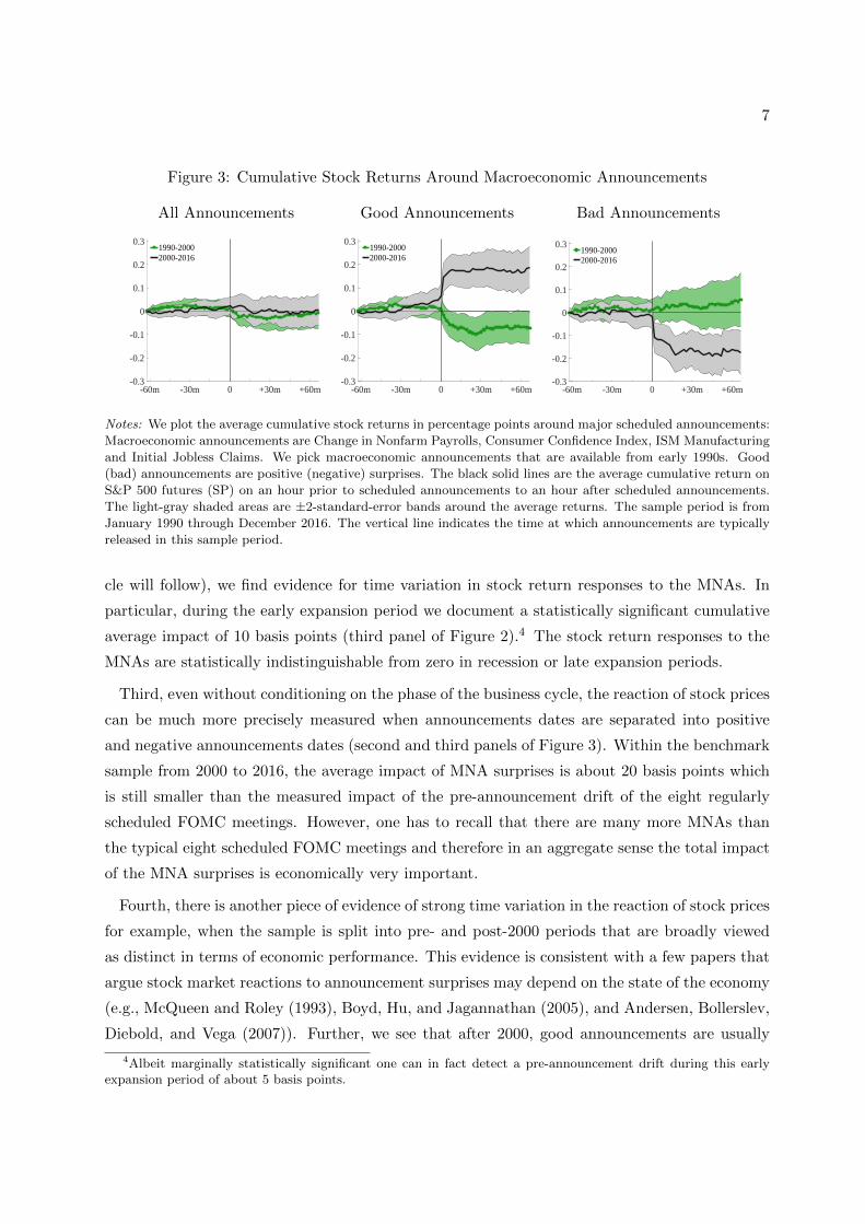
Figure 3: Cumulative Stock Returns Around Macroeconomic Announcements
All Announcements Good Announcements Bad Announcements
-60m -30m 0 +30m +60m-0.3
-0.2
-0.1
0
0.1
0.2
0.31990-20002000-2016
-60m -30m 0 +30m +60m-0.3
-0.2
-0.1
0
0.1
0.2
0.31990-20002000-2016
-60m -30m 0 +30m +60m-0.3
-0.2
-0.1
0
0.1
0.2
0.31990-20002000-2016
Notes: We plot the average cumulative stock returns in percentage points around major scheduled announcements:
Macroeconomic announcements are Change in Nonfarm Payrolls, Consumer Confidence Index, ISM Manufacturing
and Initial Jobless Claims. We pick macroeconomic announcements that are available from early 1990s. Good
(bad) announcements are positive (negative) surprises. The black solid lines are the average cumulative return on
S&P 500 futures (SP) on an hour prior to scheduled announcements to an hour after scheduled announcements.
The light-gray shaded areas are ±2-standard-error bands around the average returns. The sample period is from
January 1990 through December 2016. The vertical line indicates the time at which announcements are typically
released in this sample period.
cle will follow), we find evidence for time variation in stock return responses to the MNAs. In
particular, during the early expansion period we document a statistically significant cumulative
average impact of 10 basis points (third panel of Figure 2).4 The stock return responses to the
MNAs are statistically indistinguishable from zero in recession or late expansion periods.
Third, even without conditioning on the phase of the business cycle, the reaction of stock prices
can be much more precisely measured when announcements dates are separated into positive
and negative announcements dates (second and third panels of Figure 3). Within the benchmark
sample from 2000 to 2016, the average impact of MNA surprises is about 20 basis points which
is still smaller than the measured impact of the pre-announcement drift of the eight regularly
scheduled FOMC meetings. However, one has to recall that there are many more MNAs than
the typical eight scheduled FOMC meetings and therefore in an aggregate sense the total impact
of the MNA surprises is economically very important.
Fourth, there is another piece of evidence of strong time variation in the reaction of stock prices
for example, when the sample is split into pre- and post-2000 periods that are broadly viewed
as distinct in terms of economic performance. This evidence is consistent with a few papers that
argue stock market reactions to announcement surprises may depend on the state of the economy
(e.g., McQueen and Roley (1993), Boyd, Hu, and Jagannathan (2005), and Andersen, Bollerslev,
Diebold, and Vega (2007)). Further, we see that after 2000, good announcements are usually
4Albeit marginally statistically significant one can in fact detect a pre-announcement drift during this earlyexpansion period of about 5 basis points.

8
good for the stock market and bad announcements are usually bad. This is markedly different
from the 1990s where good (bad) announcements are usually bad (good) as emphasized in the
earlier literature.
Collectively, Figure 2 and Figure 3 emphasize the importance of accounting for time variation
and highlight the difficulty of measuring the impact of the MNA surprises on stock market.
To gain better econometric power in identifying the stock market responses, we proceed with a
regression analysis.
2.3 Main Analysis
To measure the effect of the MNA surprises on stock prices, we take the intra-day future prices and
compute returns rt in a ∆-minute window around the surprises. For our benchmark results, we
use the ES contract to measure stock returns because it is most actively traded during the MNA
release times. To determine which MNAs impact returns, we estimate the following regression
motivated by Gurkaynak, Sack, and Swanson (2005) and others
rt+∆ht−∆l
= α+ γ>Xt + εt (1)
where the vector Xt contains various MNA surprises. We proceed by first determining the most
impactful announcements across various window intervals, then select the return window, and
then focus on the cyclicality of the return response.
As the results can depend on the size of the return window, we consider all combinations of ∆l
and ∆h between 10 minutes and 90 minutes in increments of 10 minutes (81 regressions in total).5
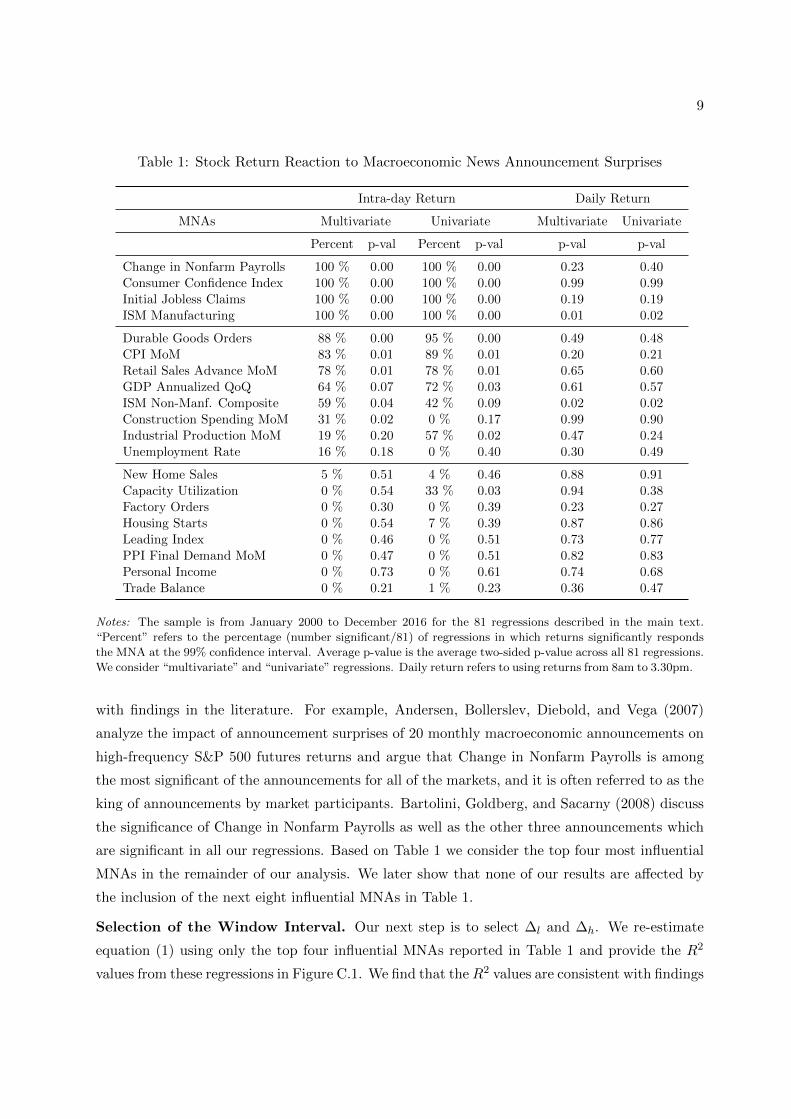
Table 1 tabulates the number of regressions in which equity returns significantly respond to a
specific MNA at the 99% confidence interval. For instance, the Unemployment Rate surprise is
significant in 16% of these regressions. We use many combinations of the return window precisely
because the significance of the MNAs depends on the size of the return window, see for example,
Andersen, Bollerslev, Diebold, and Vega (2003) and Bartolini, Goldberg, and Sacarny (2008).
This is confirmed in Table 1. This step allows us to select the MNAs while being agnostic over
the size of the return window.
Selection of the Macroeconomic News Announcement Surprises. We now turn to the
selection of the MNAs. Table 1 reveals that only a subset of the MNAs impacts the stock market.
We find that Change in Nonfarm Payrolls, Initial Jobless Claims, ISM Manufacturing, Consumer
Confidence Index Consistent are, broadly speaking, the most influential MNAs. This is consistent
5Bollerslev, Law, and Tauchen (2008) show that sampling too finely introduces micro-structure noise whilesampling too infrequently confounds the effects of the MNA surprise with all other factors aggregated into stockprices over the time interval.
9
Table 1: Stock Return Reaction to Macroeconomic News Announcement Surprises
Intra-day Return Daily Return
MNAs Multivariate Univariate Multivariate Univariate
Percent p-val Percent p-val p-val p-val
Change in Nonfarm Payrolls 100 % 0.00 100 % 0.00 0.23 0.40Consumer Confidence Index 100 % 0.00 100 % 0.00 0.99 0.99Initial Jobless Claims 100 % 0.00 100 % 0.00 0.19 0.19ISM Manufacturing 100 % 0.00 100 % 0.00 0.01 0.02
Durable Goods Orders 88 % 0.00 95 % 0.00 0.49 0.48CPI MoM 83 % 0.01 89 % 0.01 0.20 0.21Retail Sales Advance MoM 78 % 0.01 78 % 0.01 0.65 0.60GDP Annualized QoQ 64 % 0.07 72 % 0.03 0.61 0.57ISM Non-Manf. Composite 59 % 0.04 42 % 0.09 0.02 0.02Construction Spending MoM 31 % 0.02 0 % 0.17 0.99 0.90Industrial Production MoM 19 % 0.20 57 % 0.02 0.47 0.24Unemployment Rate 16 % 0.18 0 % 0.40 0.30 0.49
New Home Sales 5 % 0.51 4 % 0.46 0.88 0.91Capacity Utilization 0 % 0.54 33 % 0.03 0.94 0.38Factory Orders 0 % 0.30 0 % 0.39 0.23 0.27Housing Starts 0 % 0.54 7 % 0.39 0.87 0.86Leading Index 0 % 0.46 0 % 0.51 0.73 0.77PPI Final Demand MoM 0 % 0.47 0 % 0.51 0.82 0.83Personal Income 0 % 0.73 0 % 0.61 0.74 0.68Trade Balance 0 % 0.21 1 % 0.23 0.36 0.47
Notes: The sample is from January 2000 to December 2016 for the 81 regressions described in the main text.
“Percent” refers to the percentage (number significant/81) of regressions in which returns significantly responds
the MNA at the 99% confidence interval. Average p-value is the average two-sided p-value across all 81 regressions.
We consider “multivariate” and “univariate” regressions. Daily return refers to using returns from 8am to 3.30pm.
with findings in the literature. For example, Andersen, Bollerslev, Diebold, and Vega (2007)
analyze the impact of announcement surprises of 20 monthly macroeconomic announcements on
high-frequency S&P 500 futures returns and argue that Change in Nonfarm Payrolls is among
the most significant of the announcements for all of the markets, and it is often referred to as the
king of announcements by market participants. Bartolini, Goldberg, and Sacarny (2008) discuss
the significance of Change in Nonfarm Payrolls as well as the other three announcements which
are significant in all our regressions. Based on Table 1 we consider the top four most influential
MNAs in the remainder of our analysis. We later show that none of our results are affected by
the inclusion of the next eight influential MNAs in Table 1.
Selection of the Window Interval. Our next step is to select ∆l and ∆h. We re-estimate
equation (1) using only the top four influential MNAs reported in Table 1 and provide the R2
values from these regressions in Figure C.1. We find that theR2 values are consistent with findings
10
in the literature, for example, Andersen, Bollerslev, Diebold, and Vega (2007) and Goldberg and
Grisse (2013). For the subsequent analysis, we consider regressions with ∆ = ∆l = ∆h and
set ∆ = 30min. This symmetric window yields an R2 value of 0.13 which is representative of
the R2 distribution in Figure C.1. We emphasize that our results are maintained across all 81
combinations of ∆l and ∆h.
Cyclical Stock Return Sensitivity to News. Having fixed ∆ = 30min and restricted the
set of MNAs to the top four most influential MNAs, we now turn our attention to measuring
the time-varying sensitivity of the returns to macroeconomic news. To do this, we estimate the
following nonlinear regression over τ -period rolling windows as in Swanson and Williams (2014)
rt+∆t−∆ = ατ + βτγ>Xt + εt (2)
where εt is a residual representing the influence of other news and other factors on stock returns at
time t. ατ and βτ are scalars that capture the variation in the return response to announcement
during period τ . The underlying assumption is that while the relative magnitude of γ is constant,
the magnitude of βτ varies as the stock returns become more or less affected over time in a
proportional way across all announcement during period τ . We let τ index the calendar year.
The identification assumption is that βτ is on average equal to one. This implies that βτγ>Xt is
identical to its OLS counterpart γ>Xt in (1) on average. As discussed in Swanson and Williams
(2014), the primary advantage of this approach is that it substantially reduces the small sample
problem by bringing more data into the estimation of βτ .
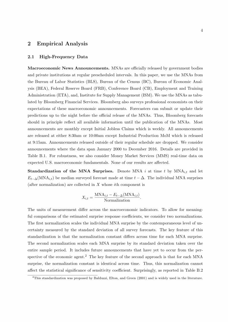
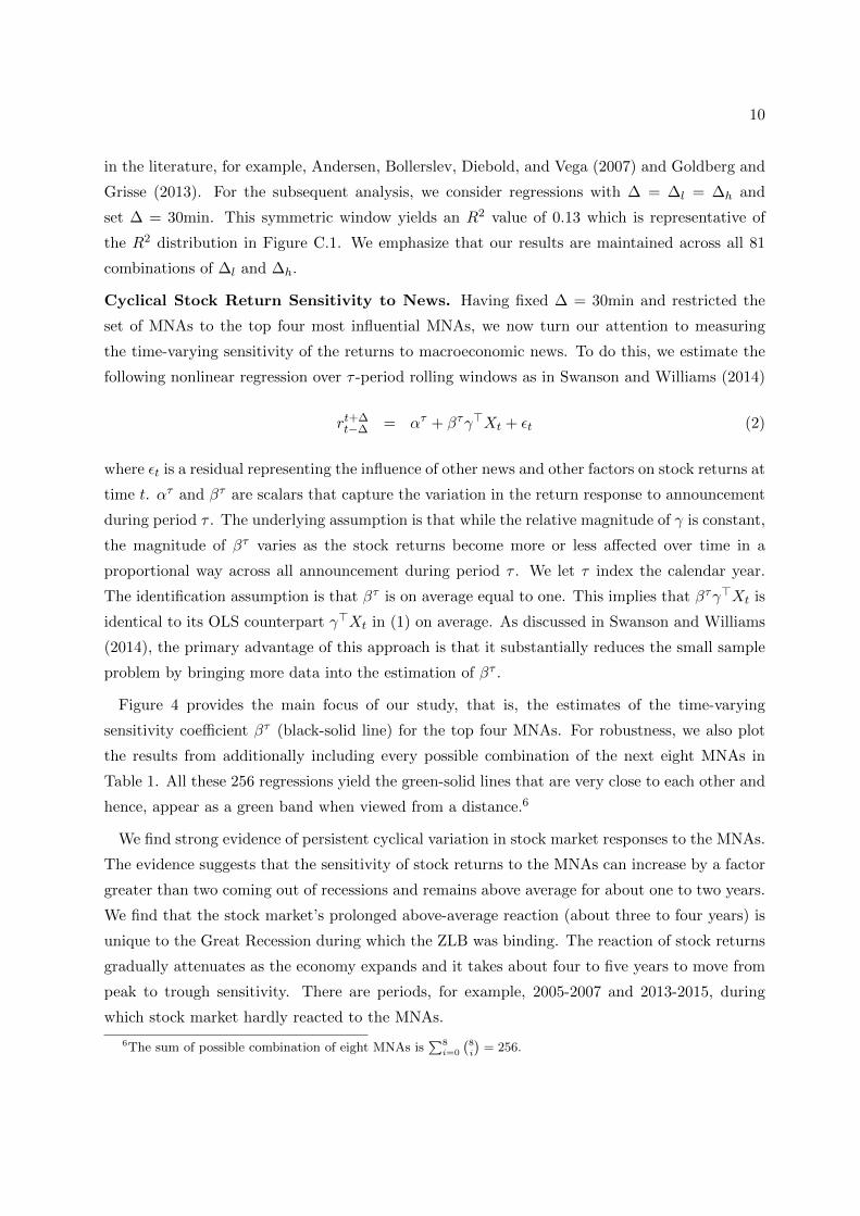
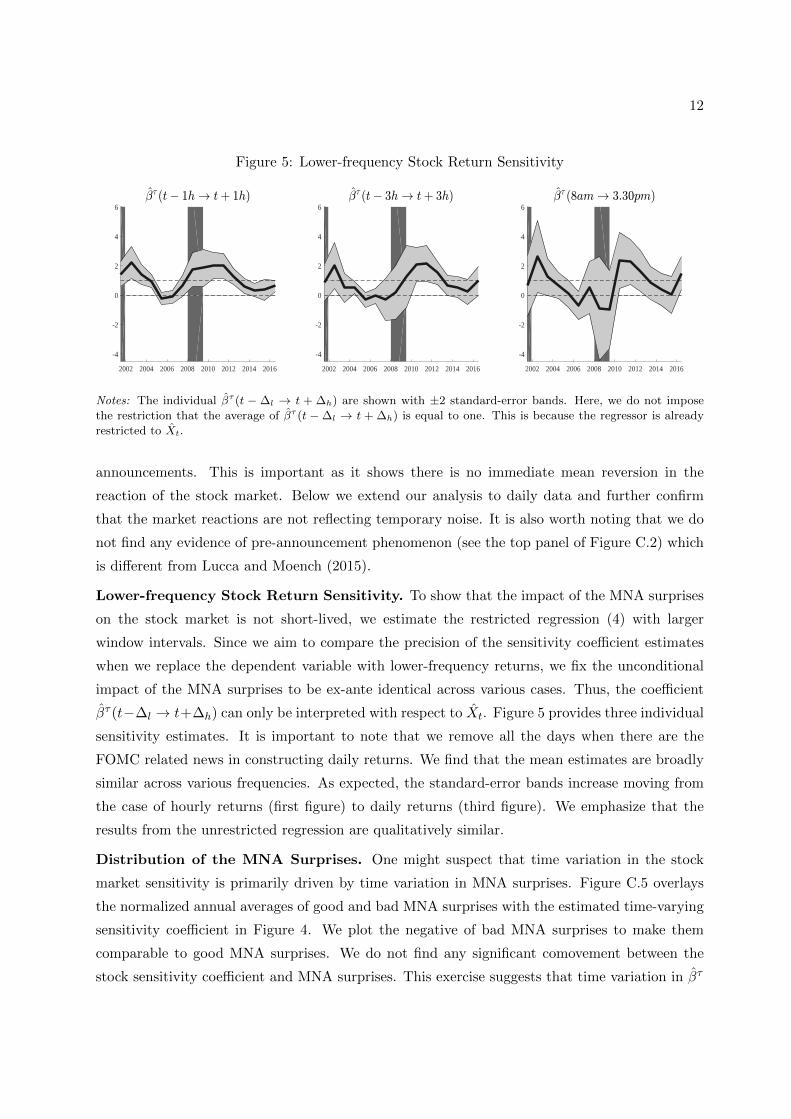
Figure 4 provides the main focus of our study, that is, the estimates of the time-varying
sensitivity coefficient βτ (black-solid line) for the top four MNAs. For robustness, we also plot
the results from additionally including every possible combination of the next eight MNAs in
Table 1. All these 256 regressions yield the green-solid lines that are very close to each other and
hence, appear as a green band when viewed from a distance.6
We find strong evidence of persistent cyclical variation in stock market responses to the MNAs.
The evidence suggests that the sensitivity of stock returns to the MNAs can increase by a factor
greater than two coming out of recessions and remains above average for about one to two years.
We find that the stock market’s prolonged above-average reaction (about three to four years) is
unique to the Great Recession during which the ZLB was binding. The reaction of stock returns
gradually attenuates as the economy expands and it takes about four to five years to move from
peak to trough sensitivity. There are periods, for example, 2005-2007 and 2013-2015, during
which stock market hardly reacted to the MNAs.
6The sum of possible combination of eight MNAs is∑8i=0
(8i
)= 256.
11
Figure 4: Time-Varying Sensitivity Coefficient for Stock Returns
2002 2004 2006 2008 2010 2012 2014 2016-1
0
1
2
3
4
Notes: The top four MNAs from Table 1 are Change in Nonfarm Payrolls, Consumer Confidence Index, Initial
Jobless Claims, and ISM Manufacturing. We impose that βτ (black-solid line) is on average equal to one. We
set ∆ = 30min. We provide ±2-standard-error bands (light-shaded area) around βτ . The shape is robust to all
possible combinations (green-solid lines) of the next eight MNAs listed in Table 1.
Pre- and Post-announcement Stock Return Sensitivity. To better understand how infor-
mation contained in the MNAs is conveyed in the stock market, we decompose βτ to sensitivity
attributable to periods before and after the announcements. To recap, the estimates from the
benchmark regression are provided below
rt+30mt−30m = ατ + βτ (γ>Xt) (3)
= ατ + βτ Xt.
We estimate the modified (restricted) regression in which we regress return rt+∆ht−∆l
on Xt
rt+∆ht−∆l
= ατ + βτ Xt + εt (4)
and obtain estimate of βτ for each combination of (∆h,∆l) ∈ −5m, 0m, 5m, 30m, which we
denote by βτ (t−∆l → t+ ∆h). The sensitivity is with respect to the linearly transformed MNA
surprises, Xt. We emphasize that we accounted for the two-stage sampling uncertainty when
constructing standard error bands. Since rt+30mt−30m =
∑rt+∆ht−∆l
, it follows that∑βτ (t−∆l → t+∆h)
in Figure C.2 equals βτ shown in Figure 4.
Figure C.2 shows that stock prices on impact react significantly to the MNA surprises (bottom
left of Figure C.2), but there is no statistically significant movement five minutes after the
12
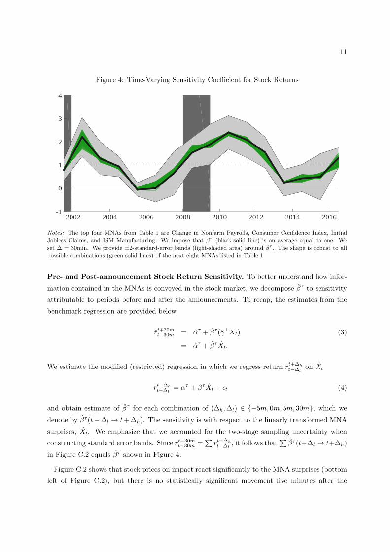
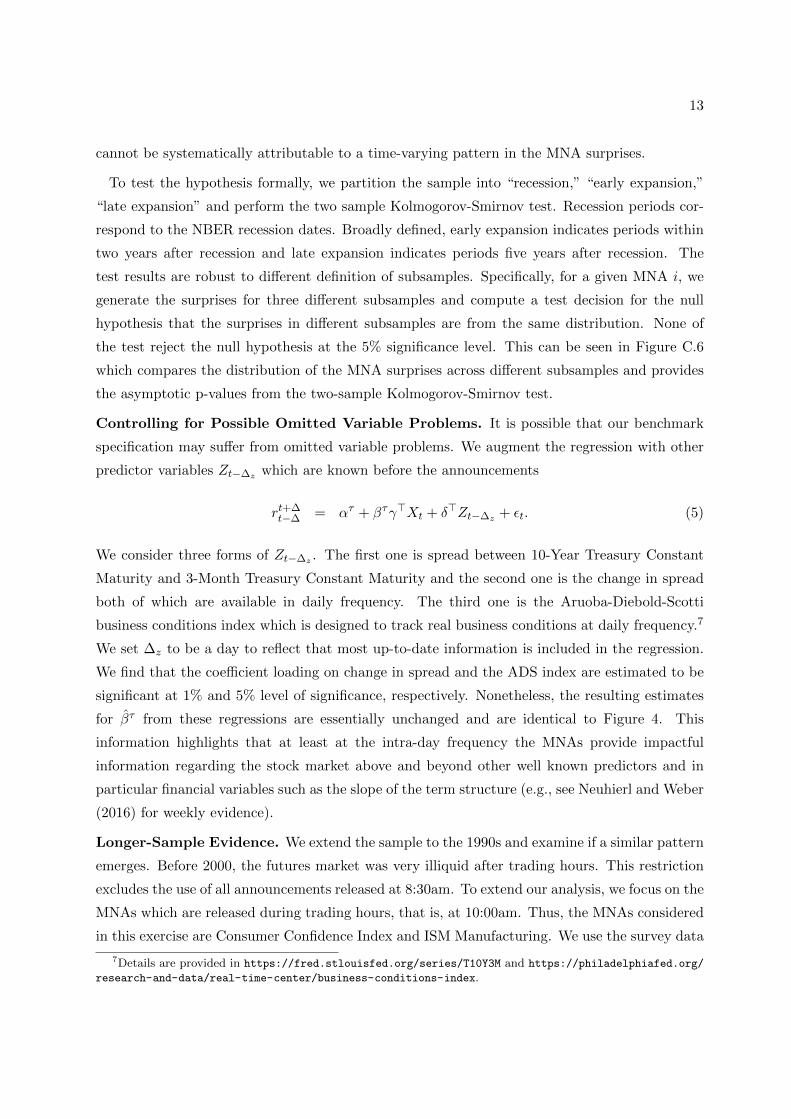
Figure 5: Lower-frequency Stock Return Sensitivity
2002 2004 2006 2008 2010 2012 2014 2016
-4
-2
0
2
4
6
2002 2004 2006 2008 2010 2012 2014 2016
-4
-2
0
2
4
6
2002 2004 2006 2008 2010 2012 2014 2016
-4
-2
0
2
4
6
Notes: The individual βτ (t − ∆l → t + ∆h) are shown with ±2 standard-error bands. Here, we do not impose
the restriction that the average of βτ (t −∆l → t + ∆h) is equal to one. This is because the regressor is already
restricted to Xt.
announcements. This is important as it shows there is no immediate mean reversion in the
reaction of the stock market. Below we extend our analysis to daily data and further confirm
that the market reactions are not reflecting temporary noise. It is also worth noting that we do
not find any evidence of pre-announcement phenomenon (see the top panel of Figure C.2) which
is different from Lucca and Moench (2015).
Lower-frequency Stock Return Sensitivity. To show that the impact of the MNA surprises
on the stock market is not short-lived, we estimate the restricted regression (4) with larger
window intervals. Since we aim to compare the precision of the sensitivity coefficient estimates
when we replace the dependent variable with lower-frequency returns, we fix the unconditional
impact of the MNA surprises to be ex-ante identical across various cases. Thus, the coefficient
βτ (t−∆l → t+∆h) can only be interpreted with respect to Xt. Figure 5 provides three individual
sensitivity estimates. It is important to note that we remove all the days when there are the
FOMC related news in constructing daily returns. We find that the mean estimates are broadly
similar across various frequencies. As expected, the standard-error bands increase moving from
the case of hourly returns (first figure) to daily returns (third figure). We emphasize that the
results from the unrestricted regression are qualitatively similar.
Distribution of the MNA Surprises. One might suspect that time variation in the stock
market sensitivity is primarily driven by time variation in MNA surprises. Figure C.5 overlays
the normalized annual averages of good and bad MNA surprises with the estimated time-varying
sensitivity coefficient in Figure 4. We plot the negative of bad MNA surprises to make them
comparable to good MNA surprises. We do not find any significant comovement between the
stock sensitivity coefficient and MNA surprises. This exercise suggests that time variation in βτ
13
cannot be systematically attributable to a time-varying pattern in the MNA surprises.
To test the hypothesis formally, we partition the sample into “recession,” “early expansion,”
“late expansion” and perform the two sample Kolmogorov-Smirnov test. Recession periods cor-
respond to the NBER recession dates. Broadly defined, early expansion indicates periods within
two years after recession and late expansion indicates periods five years after recession. The
test results are robust to different definition of subsamples. Specifically, for a given MNA i, we
generate the surprises for three different subsamples and compute a test decision for the null
hypothesis that the surprises in different subsamples are from the same distribution. None of
the test reject the null hypothesis at the 5% significance level. This can be seen in Figure C.6
which compares the distribution of the MNA surprises across different subsamples and provides
the asymptotic p-values from the two-sample Kolmogorov-Smirnov test.
Controlling for Possible Omitted Variable Problems. It is possible that our benchmark
specification may suffer from omitted variable problems. We augment the regression with other
predictor variables Zt−∆z which are known before the announcements
rt+∆t−∆ = ατ + βτγ>Xt + δ>Zt−∆z + εt. (5)
We consider three forms of Zt−∆z . The first one is spread between 10-Year Treasury Constant
Maturity and 3-Month Treasury Constant Maturity and the second one is the change in spread
both of which are available in daily frequency. The third one is the Aruoba-Diebold-Scotti
business conditions index which is designed to track real business conditions at daily frequency.7
We set ∆z to be a day to reflect that most up-to-date information is included in the regression.
We find that the coefficient loading on change in spread and the ADS index are estimated to be
significant at 1% and 5% level of significance, respectively. Nonetheless, the resulting estimates
for βτ from these regressions are essentially unchanged and are identical to Figure 4. This
information highlights that at least at the intra-day frequency the MNAs provide impactful
information regarding the stock market above and beyond other well known predictors and in
particular financial variables such as the slope of the term structure (e.g., see Neuhierl and Weber
(2016) for weekly evidence).
Longer-Sample Evidence. We extend the sample to the 1990s and examine if a similar pattern
emerges. Before 2000, the futures market was very illiquid after trading hours. This restriction
excludes the use of all announcements released at 8:30am. To extend our analysis, we focus on the
MNAs which are released during trading hours, that is, at 10:00am. Thus, the MNAs considered
in this exercise are Consumer Confidence Index and ISM Manufacturing. We use the survey data
7Details are provided in https://fred.stlouisfed.org/series/T10Y3M and https://philadelphiafed.org/
research-and-data/real-time-center/business-conditions-index.
14
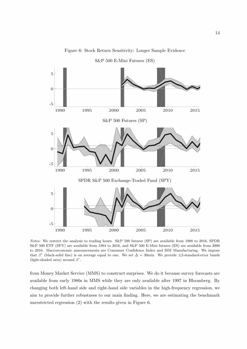
Figure 6: Stock Return Sensitivity: Longer Sample Evidence
S&P 500 E-Mini Futures (ES)
1990 1995 2000 2005 2010 2015
-5
0
5
S&P 500 Futures (SP)
1990 1995 2000 2005 2010 2015
-5
0
5
SPDR S&P 500 Exchange-Traded Fund (SPY)
1990 1995 2000 2005 2010 2015
-5
0
5
Notes: We restrict the analysis to trading hours. S&P 500 futures (SP) are available from 1988 to 2016, SPDR
S&P 500 ETF (SPY) are available from 1994 to 2016, and S&P 500 E-Mini futures (ES) are available from 2000
to 2016. Macroeconomic announcements are Consumer Confidence Index and ISM Manufacturing. We impose
that βτ (black-solid line) is on average equal to one. We set ∆ = 30min. We provide ±2-standard-error bands
(light-shaded area) around βτ .
from Money Market Service (MMS) to construct surprises. We do it because survey forecasts are
available from early 1980s in MMS while they are only available after 1997 in Bloomberg. By
changing both left-hand side and right-hand side variables in the high-frequency regression, we
aim to provide further robustness to our main finding. Here, we are estimating the benchmark
unrestricted regression (2) with the results given in Figure 6.
15
First, observe that exclusion of MNAs that are released at 8.30am, which are employment-
related announcements (Change in Nonfarm Payrolls and Initial Jobless Claims), does not alter
our main empirical findings. That is the first panel in Figure 6 is very similar to Figure 4.
Second, we find that liquidity and future rolling methods do not affect our findings. Our results
are qualitatively preserved whether we use ES or the S&P 500 Future contract (SP) or SPDR
S&P 500 Exchange Traded Funds (SPY). Hence, we conclude from Figure 6 that our empirical
findings are robust across various return measures, surprise measures, and different periods.8
Other Robustness Checks. We improve the econometric power in identifying the cyclical
variation in stock return responses by pooling information within τ period, i.e., a year. Yet,
it requires us to assume that the responses move proportionally within τ period. Figure C.3
shows that our results are robust to different smoothing parameter values τ . We also relax
the assumption that the stock return responsiveness to all MNA surprises shifts by a roughly
proportionate amount. This amounts to removing the common βτ structure in (2) and replacing
with individual γτ . Figure C.4 shows that the stock return responsiveness is qualitatively similar
across individual MNAs.
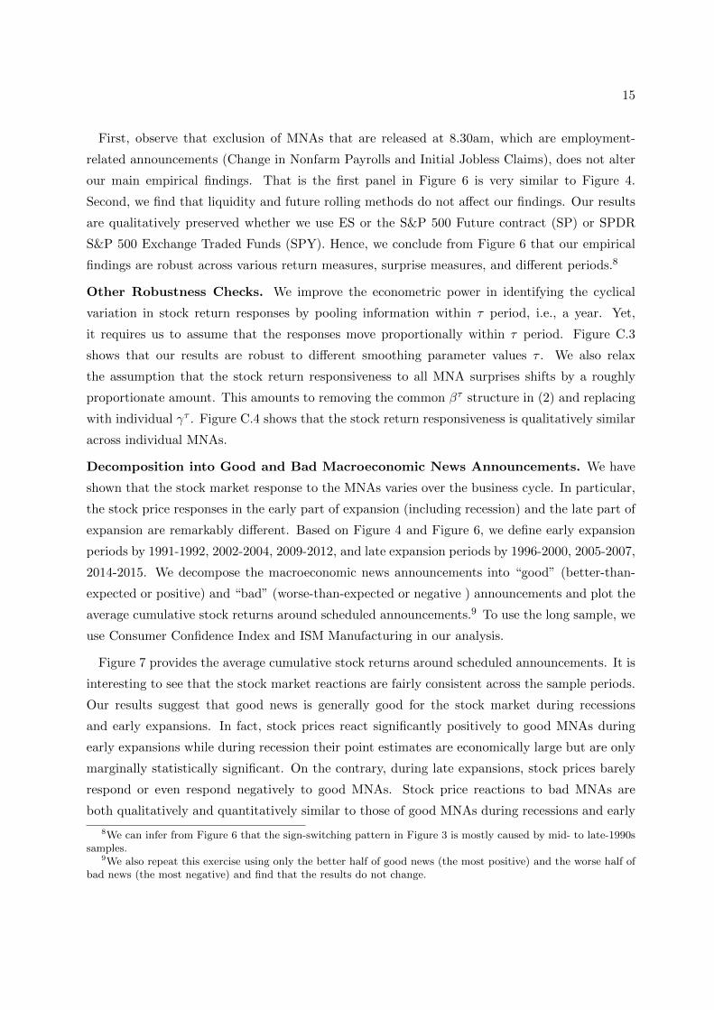
Decomposition into Good and Bad Macroeconomic News Announcements. We have
shown that the stock market response to the MNAs varies over the business cycle. In particular,
the stock price responses in the early part of expansion (including recession) and the late part of
expansion are remarkably different. Based on Figure 4 and Figure 6, we define early expansion
periods by 1991-1992, 2002-2004, 2009-2012, and late expansion periods by 1996-2000, 2005-2007,
2014-2015. We decompose the macroeconomic news announcements into “good” (better-than-
expected or positive) and “bad” (worse-than-expected or negative ) announcements and plot the
average cumulative stock returns around scheduled announcements.9 To use the long sample, we
use Consumer Confidence Index and ISM Manufacturing in our analysis.
Figure 7 provides the average cumulative stock returns around scheduled announcements. It is
interesting to see that the stock market reactions are fairly consistent across the sample periods.
Our results suggest that good news is generally good for the stock market during recessions
and early expansions. In fact, stock prices react significantly positively to good MNAs during
early expansions while during recession their point estimates are economically large but are only
marginally statistically significant. On the contrary, during late expansions, stock prices barely
respond or even respond negatively to good MNAs. Stock price reactions to bad MNAs are
both qualitatively and quantitatively similar to those of good MNAs during recessions and early
8We can infer from Figure 6 that the sign-switching pattern in Figure 3 is mostly caused by mid- to late-1990ssamples.
9We also repeat this exercise using only the better half of good news (the most positive) and the worse half ofbad news (the most negative) and find that the results do not change.
16
Figure 7: Cumulative Stock Returns Around Macroeconomic Announcements
2000-2016
Recession Early Expansion Late Expansion
-60m -30m 0 +30m +60m-0.5
0
0.5Good MNAs
-60m -30m 0 +30m +60m-0.5
0
0.5Bad MNAs
-60m -30m 0 +30m +60m
-0.5
0
0.5 Good MNAs
-60m -30m 0 +30m +60m
-0.5
0
0.5 Bad MNAs
-60m -30m 0 +30m +60m
-0.5
0
0.5 Good MNAs
-60m -30m 0 +30m +60m
-0.5
0
0.5 Bad MNAs
1990-2016
Recession Early Expansion Late Expansion
-60m -30m 0 +30m +60m-0.5
0
0.5Good MNAs
-60m -30m 0 +30m +60m-0.5
0
0.5Bad MNAs
-60m -30m 0 +30m +60m-0.5
0
0.5Good MNAs
-60m -30m 0 +30m +60m-0.5
0
0.5Bad MNAs
-60m -30m 0 +30m +60m-0.5
0
0.5Good MNAs
-60m -30m 0 +30m +60m-0.5
0
0.5Bad MNAs
Notes: We plot the average cumulative stock returns around scheduled announcements (Consumer Confidence
Index and ISM Manufacturing). We pick macroeconomic announcements that are available from early 1990s.
Good (Bad) announcements are positive (negative) surprises. Recession periods correspond to NBER recession
dates. Early expansion periods are 1991-1992, 2002-2004, 2009-2012. Late expansion periods are 1996-2000, 2005-
2007, 2014-2015. The black solid lines are the average cumulative return on S&P 500 futures (SP) on an hour
prior to scheduled announcements to an hour after scheduled announcements. The light-gray shaded areas are
±2-standard-error bands around the average returns. The sample period is from January 1990 through December
2016. The vertical line indicates the time at which announcements are released in this sample period.
expansions. Overall, it seems the responses to good and bad MNAs do not display asymmetry.10
10This is also confirmed in Figure C.10. Except 2015, the evidence for asymmetry is weak.

17
2.4 Stock Market Response to the MNAs and Monetary Policy
As stated in the outset we conjecture that the stock market response is intimately related to the
economic phase and the perception about possible Fed stabilization policy. To further explore
this connection, we first document that the relationship between the estimated response βτ and
actual interest rates. To do so, we start by overlaying the (negative) stock market sensitivity with
the annual change in the federal funds rate and with the level of federal funds rate in Figure C.7.
We then regress βτ onto the federal funds rate and its annual change. Table B.3 provides the
estimation results. Strikingly, we find that the lagged change in federal funds rate and the level
of federal funds rate can predict up to 30-50% of the stock market sensitivity βτ . The associated
slope coefficients are significantly negative.11
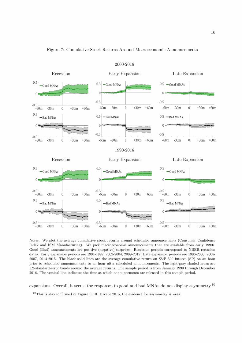
Stock Market Reaction and the Expectations of Monetary Policy. To further examine
whether the cyclical variations in the stock market’s response to the MNA surprises reflect
the market expectations of monetary policy, we next provide the time-varying sensitivity of
Eurodollar futures to the MNAs. The dependent variable is either the 3 or 6 month Euro-dollar
futures. Eurodollar futures are known to be closely related to market expectations about the
federal funds rate. We regress them on the positive and negative MNA surprises. Figure 8
display the estimated coefficients. Surprisingly, we find that the interest rate sensitivity moves
in lock-step with the stock sensitivity but in the opposite direction. This pattern is consistent
with the story that when good MNA surprises have marginal impact on the stock market, it is
because the market is worried about a future rate hike.
Several interesting episodes are noteworthy. For example, the stock sensitivity was near zero
from mid-2004 to mid-2006. From the minutes of the FOMC meetings we find that the Federal
Reserve raised the short-term interest rate in every FOMC meeting during the corresponding
periods. This is reflected in above-average interest rate sensitivity coefficients in Figure 8. 2015
was the period in which there was profound interest in the possibility of a rate hike by the Federal
Reserve.12 Note that the interest rate sensitivity was above-average for the first time since the
ZLB period. The fear about a pending rate hike caused the stock prices to go down in 2015 which
is reflected by the negative black-solid line. The opposite story holds true: when stock market
strongly reacts to good MNA surprises, it is because the market assigns a fairly low chance of a
rate hike. The entire ZLB periods are good example of the story. Overall, the evidence suggests
a tight relationship between the stock market and the expectations about monetary policy.13
11This is related to the findings in Bernanke and Kuttner (2005) where they show reversals in the direction ofrate changes have a significantly negative impact on the stock market.
12An examination of the minutes of the FOMC from 2014 confirms that a rate hike was impending. We alsoprovide compelling supportive evidence in Figure C.8 and Figure C.9.
13We are restricting our analysis to the conventional monetary policy. The effects of the unconventional monetarypolicy on financial market are studied in Swanson (2016).
18
Figure 8: Stock Market Reaction and Expectations about Monetary Policy
In Response to Good MNAs
2002 2004 2006 2008 2010 2012 2014 2016-1
0
1
2
3
4Stock FuturesEuroDollar Futures 3 MonthEuroDollar Futures 6 Month
In Response to Bad MNAs
2002 2004 2006 2008 2010 2012 2014 2016-1
0
1
2
3
4Stock FuturesEuroDollar Futures 3 MonthEuroDollar Futures 6 Month
Notes: Macroeconomic announcements are Change in Nonfarm Payrolls, Consumer Confidence Index, Initial
Jobless Claims, and ISM Manufacturing. We impose that βτ (black-solid line) is on average equal to one.
Our findings persist when we extend our analysis to data beginning 1990 which are provided in
Figure C.15.
3 Return Decomposition
Having shown the important time variation in return responses to MNAs, we further investigate
the mechanism that drives the variation in these responses. To do so, we utilize the standard
19
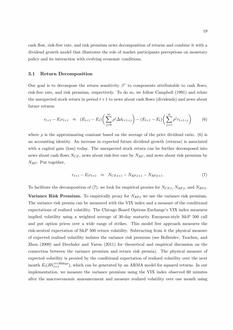
cash flow, risk-free rate, and risk premium news decomposition of returns and combine it with a
dividend growth model that illustrates the role of market participants perceptions on monetary
policy and its interaction with evolving economic conditions.
3.1 Return Decomposition
Our goal is to decompose the return sensitivity βτ to components attributable to cash flows,
risk-free rate, and risk premium, respectively. To do so, we follow Campbell (1991) and relate
the unexpected stock return in period t+1 to news about cash flows (dividends) and news about
future returns
rt+1 − Etrt+1 ≈ (Et+1 − Et)( ∞∑j=0
ρj∆dt+1+j
)− (Et+1 − Et)
( ∞∑j=1
ρjrt+1+j
)(6)
where ρ is the approximating constant based on the average of the price dividend ratio. (6) is
an accounting identity. An increase in expected future dividend growth (returns) is associated
with a capital gain (loss) today. The unexpected stock return can be further decomposed into
news about cash flows NCF , news about risk-free rate by NRF , and news about risk premium by
NRP . Put together,
rt+1 − Etrt+1 ≈ NCF,t+1 −NRF,t+1 −NRP,t+1. (7)
To facilitate the decomposition of (7), we look for empirical proxies for NCF,t, NRF,t, and NRP,t.
Variance Risk Premium. To empirically proxy for NRP,t we use the variance risk premium.
The variance risk premia can be measured with the VIX index and a measure of the conditional
expectations of realized volatility. The Chicago Board Options Exchange’s VIX index measures
implied volatility using a weighted average of 30-day maturity European-style S&P 500 call
and put option prices over a wide range of strikes. This model free approach measures the
risk-neutral expectation of S&P 500 return volatility. Subtracting from it the physical measure
of expected realized volatility isolates the variance risk premium (see Bollerslev, Tauchen, and
Zhou (2009) and Drechsler and Yaron (2011) for theoretical and empirical discussion on the
connection between the variance premium and return risk premia). The physical measure of
expected volatility is proxied by the conditional expectation of realized volatility over the next
month Et(RVt+30dayst+1 ), which can be generated by an ARMA model for squared returns. In our
implementation, we measure the variance premium using the VIX index observed 60 minutes
after the macroeconomic announcement and measure realized volatility over one month using

20
squared daily returns. The variance premium is defined by
vpt =1
Scale
(V IX2
t
12− Et(RV t+30days
t+1 )
),
scaled down appropriately to be comparable to intraday returns.14
News Decomposition. In equation (8) below, we present a state-space approach to decom-
pose equity returns into news about risk premium and news about cash flows or risk-free rate.
Specifically, we assume that the factor, Ft, is comprised of news about risk premium NRP,t and
news about the remainder
NCF,RF,t = NCF,t −NRF,t.
This is because we do not have a useful empirical proxy for either news about cash flows or news
about risk-free rate.15 Nevertheless, this approach has an important advantage in that we are
able to isolate the relative role played by news about risk premium in equity return variation.
We impose minimal sign restrictions on the factor loadings Λ whereby NRP,t is assumed to
increase (λ > 0) the variance premium and lower equity returns rtt−∆, that is, the differential of
log price at time t and log price at time t−∆. Time subscript t denotes when new macroeconomic
announcement is released. The remainder of equity return variation is explained by NCF,RF,t.
Put together,[vpt+∆
rtt−∆
]=
[λ 0
−1 1
]︸ ︷︷ ︸
Λ
[NRP,t
NCF,RF,t
]︸ ︷︷ ︸
Ft
, var(Ft) =
[σ2RP 0
0 σ2CF,RF
]. (8)
The following identity holds
rtt−∆ = −NRP,t + NCF,RF,t, (9)
where “∧” notation over a variable indicates that this value is the maximum likelihood estimate.
To connect our estimates of βτ to the decomposition of cashflow/risk free rate and risk premia
news, note that our previous regression analysis imply
rtt−∆ = ατ + βτ (γ>Xt) = ατ + βτ Xt. (10)
14We square VIX (annualized standard deviation) and divide by 12 to convert to monthly volatility.15In principle, we could use Eurodollar futures return as an empirical proxy for news about risk-free rate.
However, as we observe in Figure C.12, there is almost zero fluctuation in one-quarter ahead Eurodollar futuresreturn during 2009-2014 which contrasts starkly with the pre-crisis periods. We believe that news about risk-freerate can only be reflected in Eurodollar future contracts with much longer maturity dates, which suffer fromliquidity problems.
21
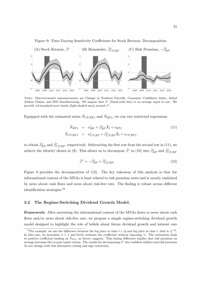
Figure 9: Time-Varying Sensitivity Coefficients for Stock Returns: Decomposition
(A) Stock Returns, βτ (B) Remainder, βτCF,RF (C) Risk Premium, −βτRP
2006 2008 2010 2012 2014 2016-1
0
1
2
3
2006 2008 2010 2012 2014 2016-1
0
1
2
3
2006 2008 2010 2012 2014 2016-1
0
1
2
3
Notes: Macroeconomic announcements are Change in Nonfarm Payrolls, Consumer Confidence Index, Initial
Jobless Claims, and ISM Manufacturing. We impose that βτ (black-solid line) is on average equal to one. We
provide ±2-standard-error bands (light-shaded area) around βτ .
Equipped with the estimated series NCF,RF,t and NRP,t, we run two restricted regressions
NRP,t = ατRP + βτRP Xt + εRP,t (11)
NCF,RF,t = ατCF,RF + βτCF,RF Xt + εCF,RF,t
to obtain βτRP and βτCF,RF , respectively. Subtracting the first row from the second row in (11), we
achieve the identity shown in (9). This allows us to decompose βτ in (10) into βτRP and βτCF,RF
βτ = −βτRP + βτCF,RF . (12)
Figure 9 provides the decomposition of (12). The key takeaway of this analysis is that the
informational content of the MNAs is least related to risk premium news and is mostly explained
by news about cash flows and news about risk-free rate. The finding is robust across different
identification strategies.16
3.2 The Regime-Switching Dividend Growth Model.
Framework. After narrowing the informational content of the MNAs down to news about cash
flows and/or news about risk-free rate, we propose a simple regime-switching dividend growth
model designed to highlight the role of beliefs about future dividend growth and interest rate
16For example, we use the difference between the log price at time t + ∆ and log price at time t, that is rt+∆t .
In this case, we normalize λ = 1 and freely estimate the coefficient without imposing -1. The estimation leadsto positive coefficient loading on NRP,t as theory suggests. This timing difference implies that risk premium onaverage increases the ex-post equity return. The results for decomposing βτ into cashflow-riskfree and risk premiumdo not change with this alternative timing and sign restriction.

22
path in accounting for stock return variation. In our simple framework, the nominal short-rate is
the monetary policy instrument and is thought to vary jointly with dividend growth. We propose
a VAR(1) dynamics in which non-neutrality of interest rate is presumed.
Dividend growth dynamics is characterized by the following state-space form
∆dt+1 = Λ0 + Λ1Zt+1, (13)
Zt+1 = Φ(St+1)Zt + Ω(St+1)xt+1, xt+1 ∼ N(0, 1),
in which the joint dynamics of (de-meaned) dividend growth and (de-meaned) risk-free rate,
Zt = [∆dt, it]′, follow a regime-switching VAR. The VAR coefficients are subject to regime
switches. Λ0 is the mean of dividend growth. Λ1 = [1, 0] is a simple selection vector. For
simplicity, we assume that there is a single shock xt that drives both dividend growth and risk-
free rate.
We consider two regimes St ∈ 1, 2 where St denotes the regime indicator variable. The
corresponding Markov transition probability matrix is provided by Π
Π =
[p11 1− p22
1− p11 p22
]
which characterizes all 22 transition probabilities. We label the first regime as the “Reactive
Monetary Policy” regime and the second regime as the “Non-Reactive Monetary Policy” regime.
1. St = 1: “Reactive Monetary Policy (R-MP)” regime (ρdi < 0, ρid > 0, φ > 0).
Φ(1) =
[ρdd ρdi
ρid ρii
], Ω(1) =
[1
φ
].
2. St = 2: “Non-Reactive Monetary Policy (NR-MP)” regime.
Φ(2) =
[ρdd 0
0 0
], Ω(2) =
[1
0
].
The sign restrictions in the R-MP regime capture the idea that a high risk-free rate hampers
future dividend growth ρdi < 0 and the risk-free rate responds positively to lagged dividend
growth ρid > 0 and to contemporaneous dividend growth shock φ > 0. We aim to incorporate
two things in the R-MP regime: non-neutrality of monetary policy (ρdi < 0) and description of
monetary policy rule (ρid > 0 and φ > 0 provide the dynamics of the risk-free rate with the
interpretation of monetary policy rule). In the R-MP regime, dividend growth shock εt+1 raises
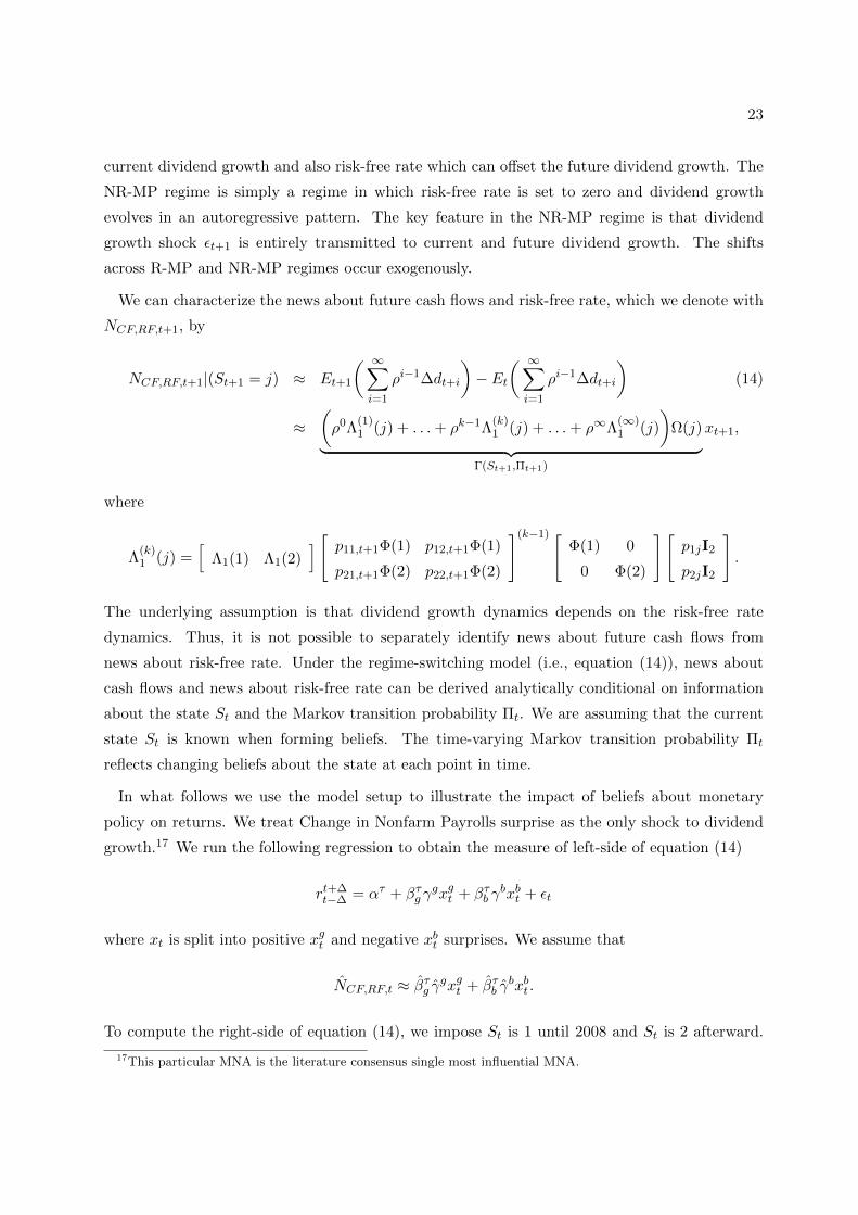
23
current dividend growth and also risk-free rate which can offset the future dividend growth. The
NR-MP regime is simply a regime in which risk-free rate is set to zero and dividend growth
evolves in an autoregressive pattern. The key feature in the NR-MP regime is that dividend
growth shock εt+1 is entirely transmitted to current and future dividend growth. The shifts
across R-MP and NR-MP regimes occur exogenously.
We can characterize the news about future cash flows and risk-free rate, which we denote with
NCF,RF,t+1, by
NCF,RF,t+1|(St+1 = j) ≈ Et+1
( ∞∑i=1
ρi−1∆dt+i
)− Et
( ∞∑i=1
ρi−1∆dt+i
)(14)
≈(ρ0Λ
(1)1 (j) + . . .+ ρk−1Λ
(k)1 (j) + . . .+ ρ∞Λ
(∞)1 (j)
)Ω(j)︸ ︷︷ ︸
Γ(St+1,Πt+1)
xt+1,
where
Λ(k)1 (j) =
[Λ1(1) Λ1(2)
] [ p11,t+1Φ(1) p12,t+1Φ(1)
p21,t+1Φ(2) p22,t+1Φ(2)
](k−1) [Φ(1) 0
0 Φ(2)
][p1jI2
p2jI2
].
The underlying assumption is that dividend growth dynamics depends on the risk-free rate
dynamics. Thus, it is not possible to separately identify news about future cash flows from
news about risk-free rate. Under the regime-switching model (i.e., equation (14)), news about
cash flows and news about risk-free rate can be derived analytically conditional on information
about the state St and the Markov transition probability Πt. We are assuming that the current
state St is known when forming beliefs. The time-varying Markov transition probability Πt
reflects changing beliefs about the state at each point in time.
In what follows we use the model setup to illustrate the impact of beliefs about monetary
policy on returns. We treat Change in Nonfarm Payrolls surprise as the only shock to dividend
growth.17 We run the following regression to obtain the measure of left-side of equation (14)
rt+∆t−∆ = ατ + βτg γ
gxgt + βτb γbxbt + εt
where xt is split into positive xgt and negative xbt surprises. We assume that
NCF,RF,t ≈ βτg γgxgt + βτb γ
bxbt .
To compute the right-side of equation (14), we impose St is 1 until 2008 and St is 2 afterward.
17This particular MNA is the literature consensus single most influential MNA.
24
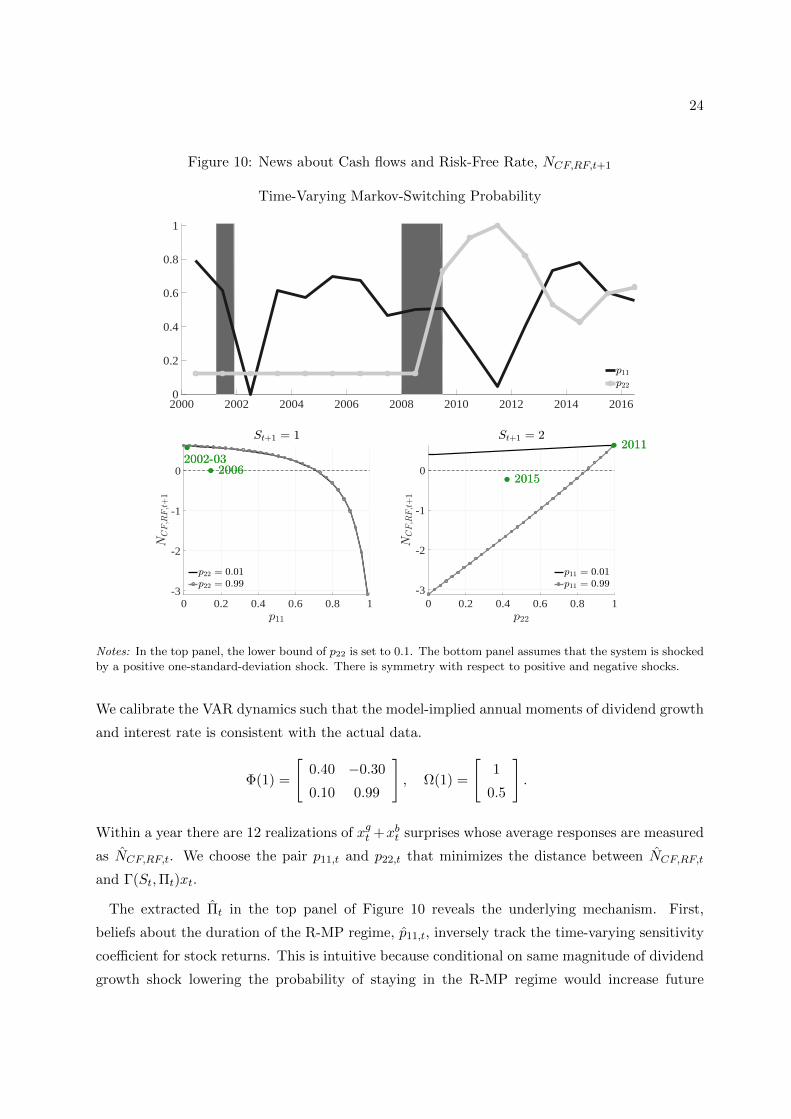
Figure 10: News about Cash flows and Risk-Free Rate, NCF,RF,t+1
Time-Varying Markov-Switching Probability
2000 2002 2004 2006 2008 2010 2012 2014 20160
0.2
0.4
0.6
0.8
1
0 0.2 0.4 0.6 0.8 1-3
-2
-1
0
0 0.2 0.4 0.6 0.8 1-3
-2
-1
0
Notes: In the top panel, the lower bound of p22 is set to 0.1. The bottom panel assumes that the system is shocked
by a positive one-standard-deviation shock. There is symmetry with respect to positive and negative shocks.
We calibrate the VAR dynamics such that the model-implied annual moments of dividend growth
and interest rate is consistent with the actual data.
Φ(1) =
[0.40 −0.30
0.10 0.99
], Ω(1) =
[1
0.5
].
Within a year there are 12 realizations of xgt +xbt surprises whose average responses are measured
as NCF,RF,t. We choose the pair p11,t and p22,t that minimizes the distance between NCF,RF,t
and Γ(St,Πt)xt.
The extracted Πt in the top panel of Figure 10 reveals the underlying mechanism. First,
beliefs about the duration of the R-MP regime, p11,t, inversely track the time-varying sensitivity
coefficient for stock returns. This is intuitive because conditional on same magnitude of dividend
growth shock lowering the probability of staying in the R-MP regime would increase future
25
dividend growth and, consequently, lead to higher stock returns. Second, the beliefs about the
NR-MP regime, p22,t, after 2009 closely match the New York Fed’s Survey of Primary Dealers in
Figure C.8. Consistent with the survey evidence, we find that the probability of staying in the
NR-MP regime was below half in 2015.
The bottom panel of Figure 10 computes (14) as functions of the Markov transition proba-
bilities. We want to use this illustrative model to show that, as in the data, the risks of an
interest rate hike (drop in p22,t or increase in transition probability from the NR-MP to the
R-MP regime) could entirely mitigate the effect of good dividend growth shocks (actual data
is highlighted by green dots). On the left-hand-side, when the state is R-MP it is evident that
NCF,RF,t will be positive (i.e., positive return) only when the probability of remaining in this
R-MP state is sufficiently low. Indeed consistent with this intuition, during the post recession
years in 2002-03, NCF,RF,t is positive as the extracted p11,t is close to zero during those year (top
panel). The right hand side in the bottom panel illustrates that for large p11,t values NCF,RF
can turn negative even for relatively large p22,t. Loosely speaking, reasonable chances of moving
from the NR-MP to R-MP are enough to generate a negative effect. During the post recession
year of 2011 when the extracted p22,t is close to one and p11,t is close to zero, we observe that
returns respond positively to good dividend growth shocks. On the other hand, in 2015 when
the market perception of a reactive monetary policy substantially increase (that is, the extracted
p11,t increase immensely) the resulting reaction is negative.
4 Asset Pricing Model
The previous section highlights the interaction of cashflow news, monetary policy, and return
innovation within a reduced form model. In this section we demonstrate that similar intuition
can be extended to a modern dynamic (regime-switching) asset-pricing model, which we calibrate
to consumption and interest rate dynamics.
Real Endowments and Monetary Policy. We assume that the Federal Reserve can di-
rectly control the real rate, rt. The monetary policy rule responds to expected consumption
growth and the strength with which the Federal Reserve tries to pursue its goal—a stabilization
policy—changes over time. Stabilization policy is “aggressive” or “loose” depending on its re-
sponsiveness to consumption fluctuations. We capture this time variation with a regime-switching
policy coefficient, φ(St). To generate monetary non-neutrality, we assume that the dynamics of

26
expected consumption growth resembles the standard New Keynesian IS curve:
xt = Etxt+1 − λ(St)rt + ux,t (15)
rt = φ(St)xt + ur,t.
We impose that λ(St) ≥ 0 governs the extent to which the real rate affects expected consumption
growth. There are two shocks (both serially correlated) in this economy. One is real endowment
(consumption) shock, ux,t, and the other is monetary policy shock, ur,t. While the individual
series follows an AR(1) process, we use a VAR(1) notation to describe the dynamics of[ux,t
ur,t
]=
[ρx 0
0 ρr
][ux,t−1
ur,t−1
]+
[σx 0
0 σr
][ηx,t
ηr,t
]. (16)
The persistence coefficient Φ(St) and standard deviation matrix Σ(St) may depend on regime.
We define Markov transition probability matrix by
Π =
[p11 p21
p12 p22
].
Here, pji is the probability of changing from regime i to regime j, ∀i, j ∈ 1, 2.
By plugging the second equation in (15) to the first equation in (15), the system reduces to a
single regime-dependent equation
χ(St)xt = Etxt+1 + Λ(St)ut (17)
where
χ(St) = 1 + λ(St)φ(St), Λ(St) =[
1, −λ(St)], ut =
[ux,t ur,t
]′.
Solution. There exists a unique bounded regime-dependent linear solutions of the form
xt = Ψ(St)ut (18)
for p11 ∈ [0, 1] and p22 ∈ [0, 1) (see Davig and Leeper (2007) for a detailed discussion). The
expressions for Ψ(St) are given in Appendix E. It suffices to emphasize that Ψ(St) depends on
the current regime and expectations of monetary policy aggressiveness throughout the future
path of the economy.

27
Table 2: Calibration
Preference Shocks Consumption Policy
δ 0.999 ρx 0.4 µc 0.0016 λ(1) 0.1ψ 1.5 ρr 0.9 σ 0.0020 λ(2) 0.0γ 8.0 σx 0.0020 φ(1) 0.2
σr 0.0015 φ(2) 0.0
Notes: The model frequency is monthly. The model is calibrated to match the first three moments of annual
consumption growth.
Asset Pricing. Assume that agents have recursive preferences
mt+1 = θ log δ − θ
ψ∆ct+1 + (θ − 1)rc,t+1 (19)
where rc,t+1 is the return on all invested wealth, γ is risk aversion, ψ is intertemporal elasticity
of substitution, θ = 1−γ1−1/ψ . Suppose that realized consumption growth follows
∆ct+1 = µ+ xt + σηt+1 (20)
where xt is defined in (18). Combining (16), (18), (19), and (20), the return on all invested
wealth can be expressed by
rc,t+1 − Etrc,t+1 ≈ κ1A1(St+1)Σ(St+1)ηt+1 (21)
where κ1 is the Campbell and Shiller (1988) log linearization constant. The equilibrium solution
coefficient A1(St+1), which describes the dynamics of the price-consumption ratio, is determined
by the preference, consumption, and monetary policy parameters and is obtained from
Et(mt+1 + rc,t+1) +1
2V art(mt+1 + rc,t+1).
Model Implication. The calibrated parameter values are reported in Table 2 and are chosen
to broadly capture key moments of consumption growth data and joint interest rate dynamics.18.
In the second regime, real rate has no bearing on expected consumption growth as indicated by
λ(2) = 0. The monetary policy rule does not respond to expected consumption growth in this
regime, φ(2) = 0. To build intuition, we show the impulse responses of expected consumption
growth to real endowment ux,t and monetary policy ur,t shocks when regimes are fixed in the first
panel of Figure 11. As expected, impulse responses of expected consumption growth to monetary
18Note that in the model the autocorrelation of ux is not the autocorrelation of xt
28
Figure 11: Response of Returns and Consumption Growth
Expected Consumption Growth Response (Fixed-Regime)
10 20 30 40
0
1
2
3
4
10 20 30 40-1
-0.8
-0.6
-0.4
-0.2
0
Return Response to Both Shocks (Regime-Switching)
0 0.2 0.4 0.6 0.8 1-0.1
0
0.1
0.2
0 0.2 0.4 0.6 0.8 1-0.1
0
0.1
0.2
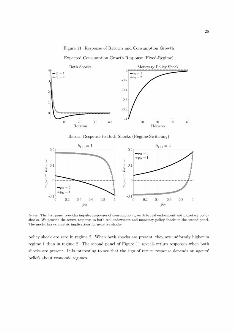
Notes: The first panel provides impulse responses of consumption growth to real endowment and monetary policy
shocks. We provide the return response to both real endowment and monetary policy shocks in the second panel.
The model has symmetric implications for negative shocks.
policy shock are zero in regime 2. When both shocks are present, they are uniformly higher in
regime 1 than in regime 2. The second panel of Figure 11 reveals return responses when both
shocks are present. It is interesting to see that the sign of return response depends on agents’
beliefs about economic regimes.

29
5 Conclusion
Using high-frequency stock returns, we provide strong evidence of persistent cyclical variation in
the sensitivity of stock prices to MNA surprises. Starting from a phase where the stock market is
insensitive to news, it becomes increasingly sensitive as the economy enters a recession with peak
sensitivity obtained a year after the recession ensued. As the economy expands, the sensitivity
comes down to its starting point in four to five years. We then provide evidence that the direction
and shape of the market’s response reflect the evolution of beliefs about monetary policy proxied
by the short-term interest rates. Specifically, we show that the sensitivity of short-term interest
rate futures to MNA surprises moves in lock-step with the stock sensitivity but in the opposite
direction. The new empirical facts are robust to various measures of stock market returns and
combinations of MNAs. Using standard return decomposition into cash flow, risk-free rate, and
risk premium news, we show that in fact, the news about future cash flows and risk-free rates are
the primary drivers of the cyclical variations. We provide a simple regime-switching model, which
is then also extended to a dynamic asset-pricing framework, in which beliefs over the duration of
monetary regimes drive the sensitivity of returns to news surprises. The model’s qualitative fit to
the data highlights that market’s beliefs over monetary policy regimes can explain the empirical
facts we present in this paper.
References
Andersen, T., T. Bollerslev, F. Diebold, and C. Vega (2003): “Micro Effects of Macro
Announcements: Real-Time Price Discovery in Foreign Exchange,” American Economic Re-
view, 93(1), 38–62.
Andersen, T., T. Bollerslev, F. Diebold, and C. Vega (2007): “Real-time Price Dis-
covery in Global Stock, Bond and Foreign Exchange Markets,” Journal of International Eco-
nomics, 73(2), 251–277.
Balduzzi, P., E. Elton, and C. Green (2001): “Economic News and Bond Prices: Evidence
from the U.S. Treasury Market,” Journal of Financial and Quantitative Analysis, 36, 523–543.
Bartolini, L., L. S. Goldberg, and A. Sacarny (2008): “How Economic News Moves
Markets,” Federal Reserve Bank of New York Current Issues in Economics and Finance, 14,
1–7.
Bekaert, G., M. Hoerova, and M. Lo Duca (2013): “Risk, Uncertainty and Monetary
Policy,” Journal of Monetary Economics, 60, 771–788.
Bernanke, B., and K. Kuttner (2005): “What Explains the Stock Market’s Reaction to
Federal Reserve Policy?,” Journal of Finance, 60(3), 1221–1257.
Bollerslev, T., T. Law, and G. Tauchen (2008): “Risk, Jumps, and Diversification,”
Journal of Econometrics, 144, 234–256.
Bollerslev, T., G. Tauchen, and H. Zhou (2009): “Expected Stock Returns and Variance
Risk Premia,” Review of Financial Studies, 22(11), 4463–4492.
Boyd, J., J. Hu, and R. Jagannathan (2005): “The Stock Markets Reaction to Unemploy-
ment News: Why Bad News Is Usually Good for Stocks,” Journal of Finance, 60, 649–672.
Campbell, J. (1991): “A Variance Decomposition for Stock Returns,” Economic Journal, 101,
157–179.
Campbell, J., and R. Shiller (1988): “The Dividend-Price Ratio and Expectations of Future
Dividends and Discount Factors,” Review of Financial Studies, 1, 195–227.
Cieslak, A., and A. Vissing-Jorgensen (2017): “The Economics of the Fed Put,” Working
Paper.
Cochrane, J., and M. Piazzesi (2002): “The Fed amd Interest Rates: A High-Frequency
Identification,” American Economic Review Papers and Proceedings, 92, 90–95.
31
Davig, T., and E. Leeper (2007): “Generalizing the Taylor Principle,” American Economic
Review, 97, 607–635.
Drechsler, I., and A. Yaron (2011): “What’s Vol Got to Do With It,” Review of Financial
Studies, 24, 1–45.
Flannery, M. J., and A. A. Protopapadakis (2002): “Macroeconomic Factors Do Influence
Aggregate Stock Returns,” Review of Financial Studies, 15(3), 751–782.
Goldberg, D., and C. Grisse (2013): “Time Variation in Asset Price Responses to Macro
Announcements,” Federal Reserve Bank of New York Staff Report No. 626.
Gurkaynak, R., R. Rigobon, and B. Sack (2005): “Do Actions Speak Louder than Words?
The Response of Asset Prices to Monetary Policy Actions and Statements,” International
Journal of Central Banking, 1, 55–93.
Gurkaynak, R., B. Sack, and E. Swanson (2005): “The excess sensitivity of long-term
interest rates: evidence and implications for macroeconomic models,” American Economic
Review, 95(1), 425–36.
Lucca, D., and E. Moench (2015): “The Pre-FOMC Announcement Drift,” Journal of Fi-
nance, 70, 329–371.
McQueen, G., and V. V. Roley (1993): “Stock Prices, News, and Business Conditions,”
Review of Financial Studies, 6(3), 683–707.
Neuhierl, A., and M. Weber (2016): “Monetary Policy and the Stock Market: Time-
Series Evidence,” Working Paper 22831, National Bureau of Economic Research, DOI:
10.3386/w22831.
Pearce, D., and V. Roley (1985): “Stock Prices and Economic News,” Journal of Business,
58, 49–67.
Rigobon, R., and B. Sack (2003): “Measuring the Reaction of Monetary Policy to the Stock
Market,” Quarterly Journal of Economics, 118, 639–669.
Rigobon, R., and B. Sack (2004): “The Impact of Monetary Policy on Asset Prices,” Journal
of Monetary Economics, 51, 1553–1575.
Savor, P., and M. Wilson (2013): “How Much Do Investors Care About Macroeconomic Risk?
Evidence from Scheduled Economic Announcements,” Journal of Financial and Quantitative
Analysis, 48, 343–375.

32
Swanson, E. (2016): “Measuring the Effects of Federal Reserve Forward Guidance and Asset
Purchases on Financial Markets,” Manuscript, University of California, Irvine.
Swanson, E., and J. C. Williams (2014): “Measuring the Effect of the Zero Lower Bound on
Medium- and Longer-Term Interest Rates,” American Economic Review, 104(10), 3154–3185.
Thorbecke, W. (1997): “On Stock Market Returns and Monetary Policy,” Journal of Finance,
52, 635–654.

Law, Song, and Yaron (2017): Online Appendix A-1
Appendix
A High-Frequency Regression
For macroeconomic indicator yi,t, the standardized news variable at time t is
Xi,t =yi,t − Et−∆(yi,t)
σ(yi,t − Et−∆(yi,t))
where Et−∆(yi,t) is the mean survey expectation which was taken at t − ∆. For illustrative
purpose, assume (1) two macroeconomic variables; (2) quarterly announcements (4 per a year);
(3) 3 years of announcement data. We represent the quarterly time subscript t as t = 12(a−1)+q,
where q = 1, ..., 4. We consider the following nonlinear least squares specification
Ra,q = αa + βa
(γ1X1,a,q + γ2X2,a,q
)+ εa,q,
where q is the quarterly time subscript and a the annual time subscript. This nonlinear regression
can be expressed as
R1,1
R1,2
R1,3
R1,4
R2,1
R2,2
R2,3
R2,4
R3,1
R3,2
R3,3
R3,4
=
X1,1,1 X2,1,1 0 0 0 0 1 0 0
X1,1,2 X2,1,2 0 0 0 0 1 0 0
X1,1,3 X2,1,3 0 0 0 0 1 0 0
X1,1,4 X2,1,4 0 0 0 0 1 0 0
0 0 X1,2,1 X2,2,1 0 0 0 1 0
0 0 X1,2,2 X2,2,2 0 0 0 1 0
0 0 X1,2,3 X2,2,3 0 0 0 1 0
0 0 X1,2,4 X2,2,4 0 0 0 1 0
0 0 0 0 X1,3,1 X2,3,1 0 0 1
0 0 0 0 X1,3,2 X2,3,2 0 0 1
0 0 0 0 X1,3,3 X2,3,3 0 0 1
0 0 0 0 X1,3,4 X2,3,4 0 0 1
β1γ1
β1γ2
β2γ1
β2γ2
β3γ1
β3γ2
α1
α2
α3
+
ε1,1
ε1,2
ε1,3
ε1,4
ε2,1
ε2,2
ε2,3
ε2,4
ε3,1
ε3,2
ε3,3
ε3,4
.
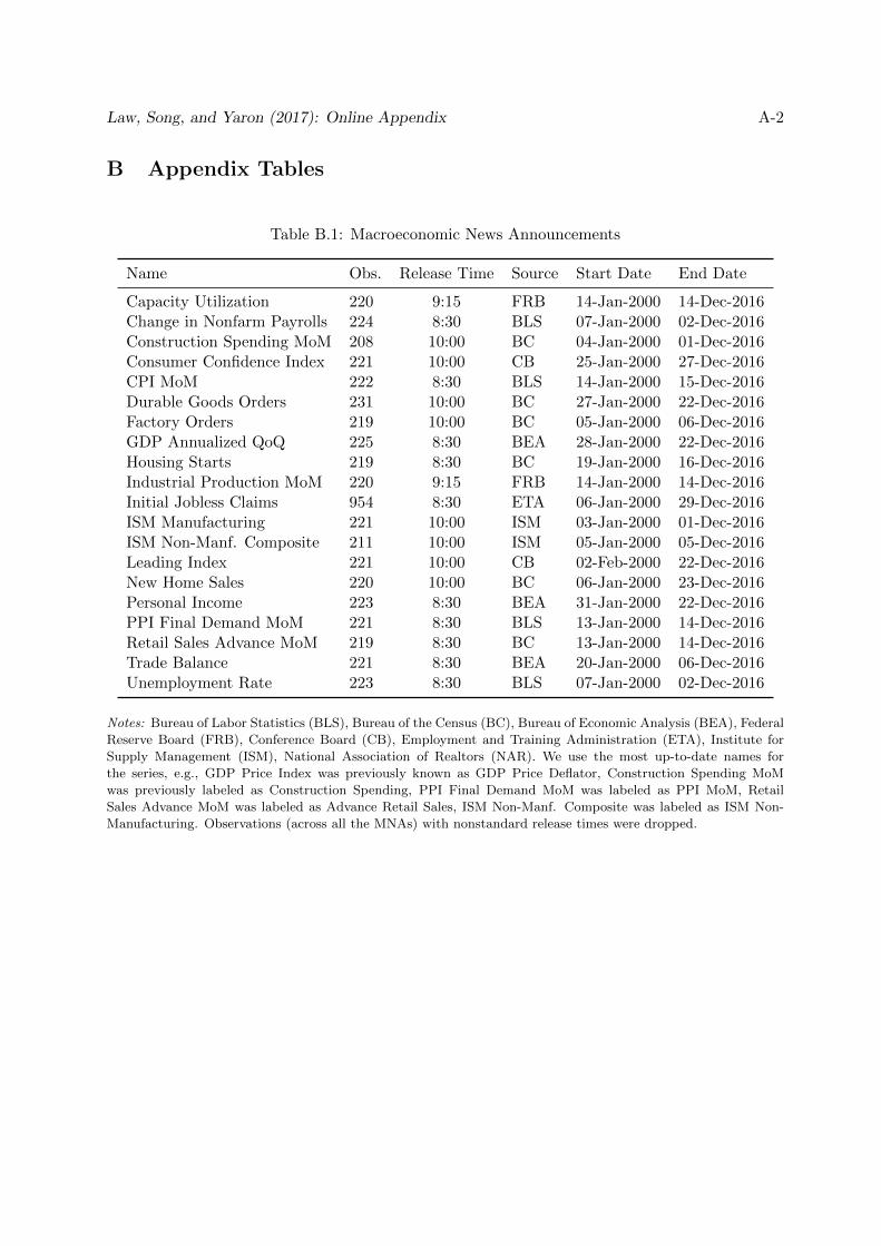
Law, Song, and Yaron (2017): Online Appendix A-2
B Appendix Tables
Table B.1: Macroeconomic News Announcements
Name Obs. Release Time Source Start Date End Date
Capacity Utilization 220 9:15 FRB 14-Jan-2000 14-Dec-2016Change in Nonfarm Payrolls 224 8:30 BLS 07-Jan-2000 02-Dec-2016Construction Spending MoM 208 10:00 BC 04-Jan-2000 01-Dec-2016Consumer Confidence Index 221 10:00 CB 25-Jan-2000 27-Dec-2016CPI MoM 222 8:30 BLS 14-Jan-2000 15-Dec-2016Durable Goods Orders 231 10:00 BC 27-Jan-2000 22-Dec-2016Factory Orders 219 10:00 BC 05-Jan-2000 06-Dec-2016GDP Annualized QoQ 225 8:30 BEA 28-Jan-2000 22-Dec-2016Housing Starts 219 8:30 BC 19-Jan-2000 16-Dec-2016Industrial Production MoM 220 9:15 FRB 14-Jan-2000 14-Dec-2016Initial Jobless Claims 954 8:30 ETA 06-Jan-2000 29-Dec-2016ISM Manufacturing 221 10:00 ISM 03-Jan-2000 01-Dec-2016ISM Non-Manf. Composite 211 10:00 ISM 05-Jan-2000 05-Dec-2016Leading Index 221 10:00 CB 02-Feb-2000 22-Dec-2016New Home Sales 220 10:00 BC 06-Jan-2000 23-Dec-2016Personal Income 223 8:30 BEA 31-Jan-2000 22-Dec-2016PPI Final Demand MoM 221 8:30 BLS 13-Jan-2000 14-Dec-2016Retail Sales Advance MoM 219 8:30 BC 13-Jan-2000 14-Dec-2016Trade Balance 221 8:30 BEA 20-Jan-2000 06-Dec-2016Unemployment Rate 223 8:30 BLS 07-Jan-2000 02-Dec-2016
Notes: Bureau of Labor Statistics (BLS), Bureau of the Census (BC), Bureau of Economic Analysis (BEA), Federal
Reserve Board (FRB), Conference Board (CB), Employment and Training Administration (ETA), Institute for
Supply Management (ISM), National Association of Realtors (NAR). We use the most up-to-date names for
the series, e.g., GDP Price Index was previously known as GDP Price Deflator, Construction Spending MoM
was previously labeled as Construction Spending, PPI Final Demand MoM was labeled as PPI MoM, Retail
Sales Advance MoM was labeled as Advance Retail Sales, ISM Non-Manf. Composite was labeled as ISM Non-
Manufacturing. Observations (across all the MNAs) with nonstandard release times were dropped.
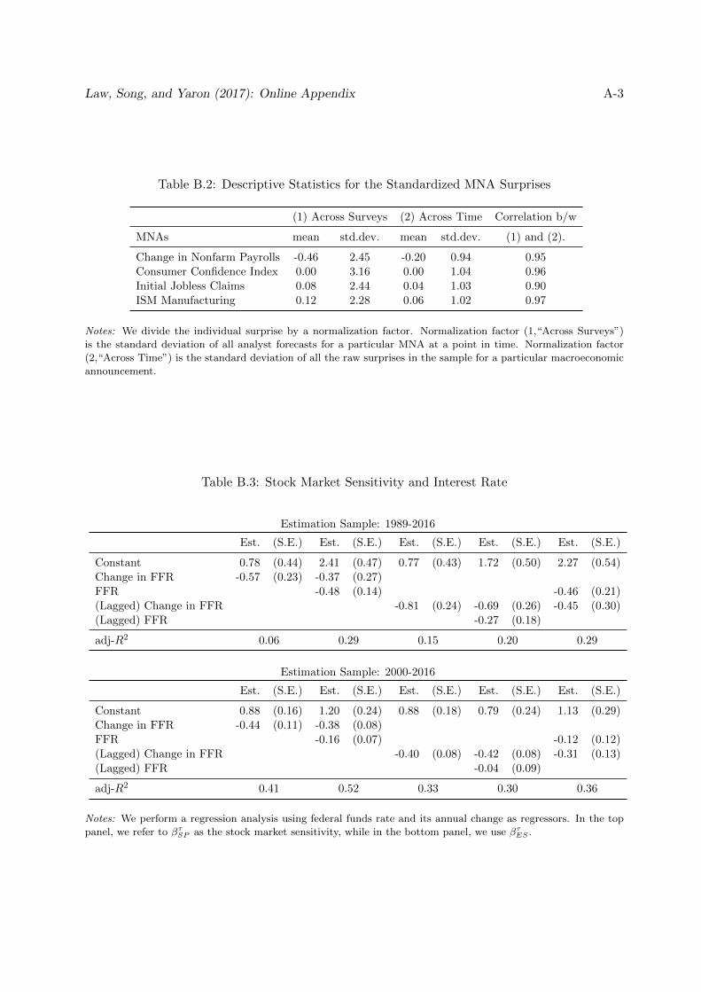
Law, Song, and Yaron (2017): Online Appendix A-3
Table B.2: Descriptive Statistics for the Standardized MNA Surprises
(1) Across Surveys (2) Across Time Correlation b/w
MNAs mean std.dev. mean std.dev. (1) and (2).
Change in Nonfarm Payrolls -0.46 2.45 -0.20 0.94 0.95Consumer Confidence Index 0.00 3.16 0.00 1.04 0.96Initial Jobless Claims 0.08 2.44 0.04 1.03 0.90ISM Manufacturing 0.12 2.28 0.06 1.02 0.97
Notes: We divide the individual surprise by a normalization factor. Normalization factor (1,“Across Surveys”)
is the standard deviation of all analyst forecasts for a particular MNA at a point in time. Normalization factor
(2,“Across Time”) is the standard deviation of all the raw surprises in the sample for a particular macroeconomic
announcement.
Table B.3: Stock Market Sensitivity and Interest Rate
Estimation Sample: 1989-2016
Est. (S.E.) Est. (S.E.) Est. (S.E.) Est. (S.E.) Est. (S.E.)
Constant 0.78 (0.44) 2.41 (0.47) 0.77 (0.43) 1.72 (0.50) 2.27 (0.54)Change in FFR -0.57 (0.23) -0.37 (0.27)FFR -0.48 (0.14) -0.46 (0.21)(Lagged) Change in FFR -0.81 (0.24) -0.69 (0.26) -0.45 (0.30)(Lagged) FFR -0.27 (0.18)
adj-R2 0.06 0.29 0.15 0.20 0.29
Estimation Sample: 2000-2016
Est. (S.E.) Est. (S.E.) Est. (S.E.) Est. (S.E.) Est. (S.E.)
Constant 0.88 (0.16) 1.20 (0.24) 0.88 (0.18) 0.79 (0.24) 1.13 (0.29)Change in FFR -0.44 (0.11) -0.38 (0.08)FFR -0.16 (0.07) -0.12 (0.12)(Lagged) Change in FFR -0.40 (0.08) -0.42 (0.08) -0.31 (0.13)(Lagged) FFR -0.04 (0.09)
adj-R2 0.41 0.52 0.33 0.30 0.36
Notes: We perform a regression analysis using federal funds rate and its annual change as regressors. In the top
panel, we refer to βτSP as the stock market sensitivity, while in the bottom panel, we use βτES .
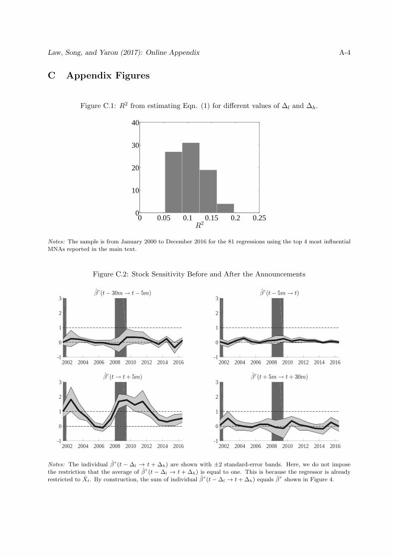
Law, Song, and Yaron (2017): Online Appendix A-4
C Appendix Figures
Figure C.1: R2 from estimating Eqn. (1) for different values of ∆l and ∆h.
0 0.05 0.1 0.15 0.2 0.250
10
20
30
40
R2
Notes: The sample is from January 2000 to December 2016 for the 81 regressions using the top 4 most influential
MNAs reported in the main text.
Figure C.2: Stock Sensitivity Before and After the Announcements
βτ (t− 30m → t− 5m)
2002 2004 2006 2008 2010 2012 2014 2016-1
0
1
2
3βτ (t− 5m → t)
2002 2004 2006 2008 2010 2012 2014 2016-1
0
1
2
3
βτ (t → t+ 5m)
2002 2004 2006 2008 2010 2012 2014 2016-1
0
1
2
3βτ (t+ 5m → t+ 30m)
2002 2004 2006 2008 2010 2012 2014 2016-1
0
1
2
3
Notes: The individual βτ (t − ∆l → t + ∆h) are shown with ±2 standard-error bands. Here, we do not impose
the restriction that the average of βτ (t −∆l → t + ∆h) is equal to one. This is because the regressor is already
restricted to Xt. By construction, the sum of individual βτ (t−∆l → t+ ∆h) equals βτ shown in Figure 4.
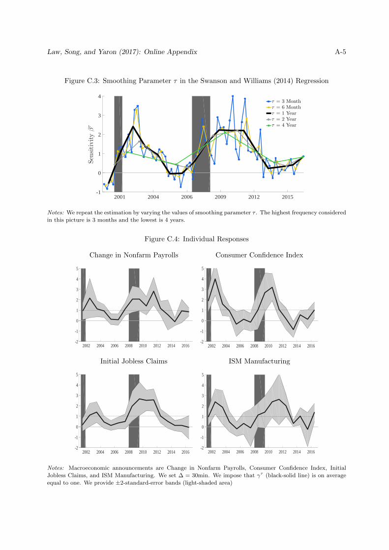
Law, Song, and Yaron (2017): Online Appendix A-5
Figure C.3: Smoothing Parameter τ in the Swanson and Williams (2014) Regression
2001 2004 2006 2009 2012 2015-1
0
1
2
3
4Sen
sitivityβτ
τ = 3 Monthτ = 6 Monthτ = 1 Yearτ = 2 Yearτ = 4 Year
Notes: We repeat the estimation by varying the values of smoothing parameter τ . The highest frequency considered
in this picture is 3 months and the lowest is 4 years.
Figure C.4: Individual Responses
Change in Nonfarm Payrolls Consumer Confidence Index
2002 2004 2006 2008 2010 2012 2014 2016-2
-1
0
1
2
3
4
5
2002 2004 2006 2008 2010 2012 2014 2016-2
-1
0
1
2
3
4
5
Initial Jobless Claims ISM Manufacturing
2002 2004 2006 2008 2010 2012 2014 2016-2
-1
0
1
2
3
4
5
2002 2004 2006 2008 2010 2012 2014 2016-2
-1
0
1
2
3
4
5
Notes: Macroeconomic announcements are Change in Nonfarm Payrolls, Consumer Confidence Index, Initial
Jobless Claims, and ISM Manufacturing. We set ∆ = 30min. We impose that γτ (black-solid line) is on average
equal to one. We provide ±2-standard-error bands (light-shaded area)
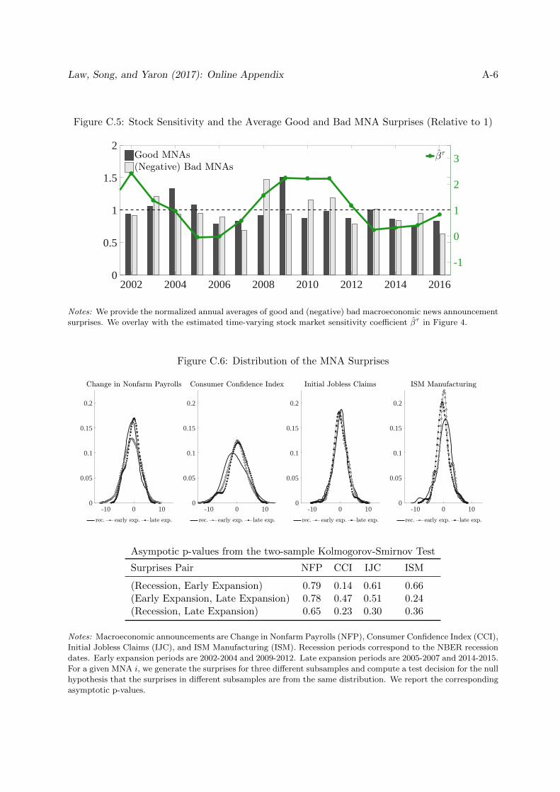
Law, Song, and Yaron (2017): Online Appendix A-6
Figure C.5: Stock Sensitivity and the Average Good and Bad MNA Surprises (Relative to 1)
2002 2004 2006 2008 2010 2012 2014 20160
0.5
1
1.5
2Good MNAs(Negative) Bad MNAs
2002 2004 2006 2008 2010 2012 2014 2016
-1
0
1
2
3βτ
Notes: We provide the normalized annual averages of good and (negative) bad macroeconomic news announcement
surprises. We overlay with the estimated time-varying stock market sensitivity coefficient βτ in Figure 4.
Figure C.6: Distribution of the MNA Surprises
-10 0 100
0.05
0.1
0.15
0.2
-10 0 100
0.05
0.1
0.15
0.2
-10 0 100
0.05
0.1
0.15
0.2
-10 0 100
0.05
0.1
0.15
0.2
Asympotic p-values from the two-sample Kolmogorov-Smirnov Test
Surprises Pair NFP CCI IJC ISM
(Recession, Early Expansion) 0.79 0.14 0.61 0.66(Early Expansion, Late Expansion) 0.78 0.47 0.51 0.24(Recession, Late Expansion) 0.65 0.23 0.30 0.36
Notes: Macroeconomic announcements are Change in Nonfarm Payrolls (NFP), Consumer Confidence Index (CCI),
Initial Jobless Claims (IJC), and ISM Manufacturing (ISM). Recession periods correspond to the NBER recession
dates. Early expansion periods are 2002-2004 and 2009-2012. Late expansion periods are 2005-2007 and 2014-2015.
For a given MNA i, we generate the surprises for three different subsamples and compute a test decision for the null
hypothesis that the surprises in different subsamples are from the same distribution. We report the corresponding
asymptotic p-values.
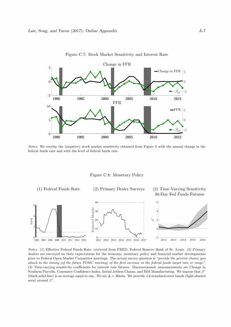
Law, Song, and Yaron (2017): Online Appendix A-7
Figure C.7: Stock Market Sensitivity and Interest Rate
1990 1995 2000 2005 2010 2015-5
0
5Change in FFR
1990 1995 2000 2005 2010 2015
-5
0
5
Change in FFR
−βτSP
1990 1995 2000 2005 2010 20150
5
10FFR
1990 1995 2000 2005 2010 2015
-5
0
5
FFR
−βτSP
Notes: We overlay the (negative) stock market sensitivity obtained from Figure 6 with the annual change in the
federal funds rate and with the level of federal funds rate.
Figure C.8: Monetary Policy
(1) Federal Funds Rate (2) Primary Dealer Surveys (3) Time-Varying Sensitivity30-Day Fed Funds Futures
2002 2004 2006 2008 2010 2012 2014 20160
2
4
6
2011 2012 2013 2014 2015 2016 20170
10
20
30
40
ExpectedMonths
2012 2013 2014 2015 2016-2
0
2
4
6
Notes: (1) Effective Federal Funds Rate, retrieved from FRED, Federal Reserve Bank of St. Louis. (2) Primary
dealers are surveyed on their expectations for the economy, monetary policy and financial market developments
prior to Federal Open Market Committee meetings. The actual survey question is “provide the percent chance you
attach to the timing (of the future FOMC meeting) of the first increase in the federal funds target rate or range.”
(3) Time-varying sensitivity coefficients for interest rate futures. Macroeconomic announcements are Change in
Nonfarm Payrolls, Consumer Confidence Index, Initial Jobless Claims, and ISM Manufacturing. We impose that βτ
(black-solid line) is on average equal to one. We set ∆ = 30min. We provide ±2-standard-error bands (light-shaded
area) around βτ .
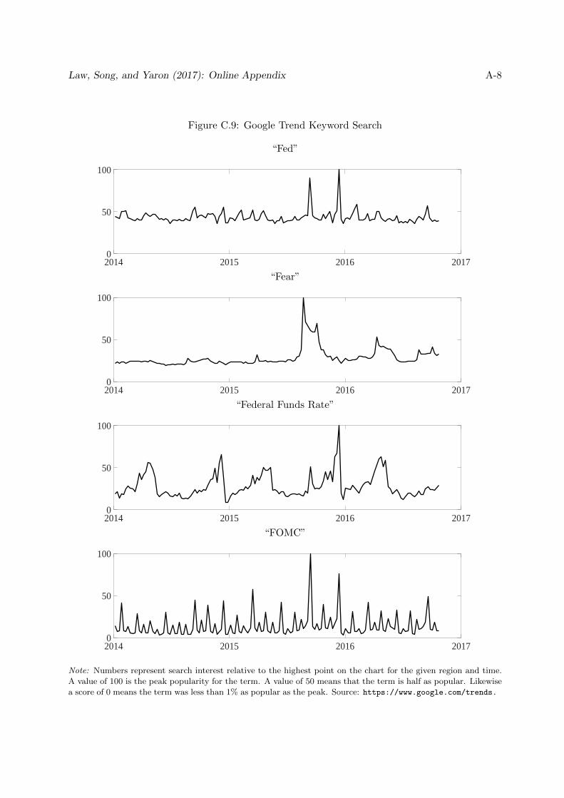
Law, Song, and Yaron (2017): Online Appendix A-8
Figure C.9: Google Trend Keyword Search
“Fed”
2014 2015 2016 20170
50
100
“Fear”
2014 2015 2016 20170
50
100
“Federal Funds Rate”
2014 2015 2016 20170
50
100
“FOMC”
2014 2015 2016 20170
50
100
Note: Numbers represent search interest relative to the highest point on the chart for the given region and time.
A value of 100 is the peak popularity for the term. A value of 50 means that the term is half as popular. Likewise
a score of 0 means the term was less than 1% as popular as the peak. Source: https://www.google.com/trends.
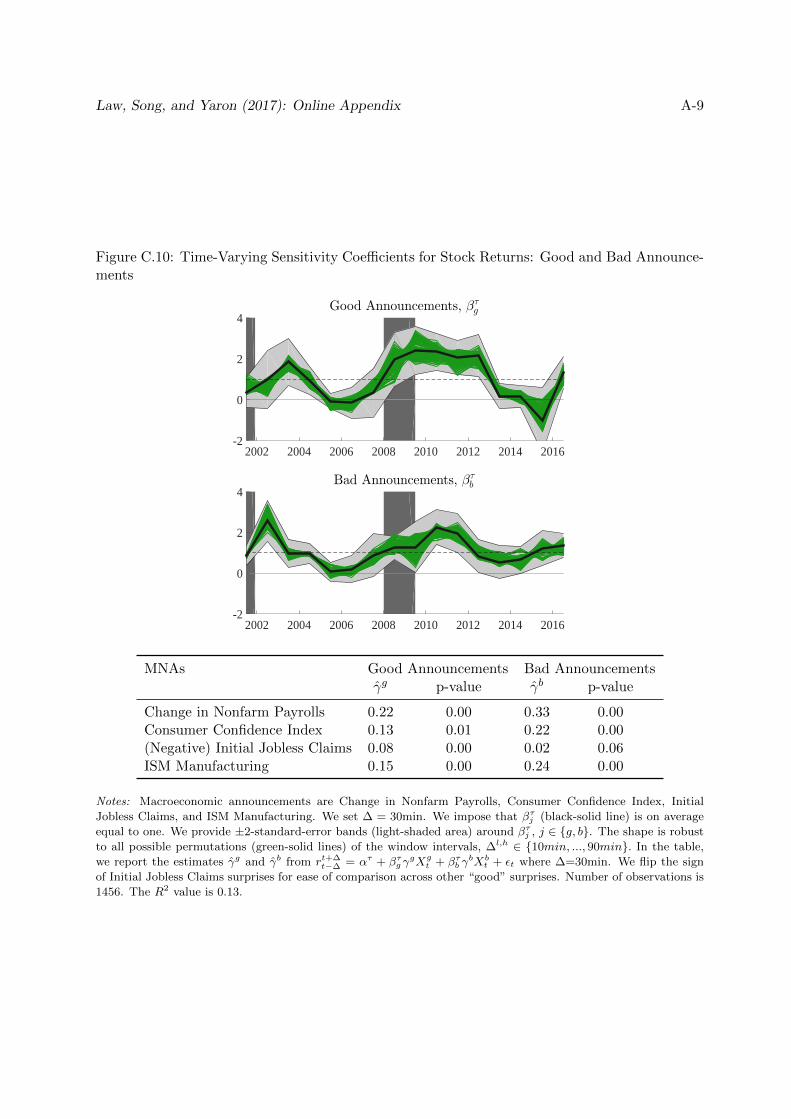
Law, Song, and Yaron (2017): Online Appendix A-9
Figure C.10: Time-Varying Sensitivity Coefficients for Stock Returns: Good and Bad Announce-ments
Good Announcements, βτg
2002 2004 2006 2008 2010 2012 2014 2016-2
0
2
4
Bad Announcements, βτb
2002 2004 2006 2008 2010 2012 2014 2016-2
0
2
4
MNAs Good Announcements Bad Announcementsγg p-value γb p-value
Change in Nonfarm Payrolls 0.22 0.00 0.33 0.00Consumer Confidence Index 0.13 0.01 0.22 0.00(Negative) Initial Jobless Claims 0.08 0.00 0.02 0.06ISM Manufacturing 0.15 0.00 0.24 0.00
Notes: Macroeconomic announcements are Change in Nonfarm Payrolls, Consumer Confidence Index, Initial
Jobless Claims, and ISM Manufacturing. We set ∆ = 30min. We impose that βτj (black-solid line) is on average
equal to one. We provide ±2-standard-error bands (light-shaded area) around βτj , j ∈ g, b. The shape is robust
to all possible permutations (green-solid lines) of the window intervals, ∆l,h ∈ 10min, ..., 90min. In the table,
we report the estimates γg and γb from rt+∆t−∆ = ατ + βτg γ
gXgt + βτb γ
bXbt + εt where ∆=30min. We flip the sign
of Initial Jobless Claims surprises for ease of comparison across other “good” surprises. Number of observations is
1456. The R2 value is 0.13.
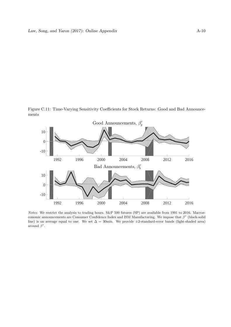
Law, Song, and Yaron (2017): Online Appendix A-10
Figure C.11: Time-Varying Sensitivity Coefficients for Stock Returns: Good and Bad Announce-ments
Good Announcements, βτg
1992 1996 2000 2004 2008 2012 2016
-10
0
10
Bad Announcements, βτb
1992 1996 2000 2004 2008 2012 2016
-10
0
10
Notes: We restrict the analysis to trading hours. S&P 500 futures (SP) are available from 1991 to 2016. Macroe-
conomic announcements are Consumer Confidence Index and ISM Manufacturing. We impose that βτ (black-solid
line) is on average equal to one. We set ∆ = 30min. We provide ±2-standard-error bands (light-shaded area)
around βτ .
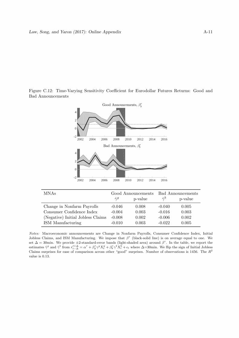
Law, Song, and Yaron (2017): Online Appendix A-11
Figure C.12: Time-Varying Sensitivity Coefficient for Eurodollar Futures Returns: Good andBad Announcements
2002 2004 2006 2008 2010 2012 2014 2016-2
0
2
4
2002 2004 2006 2008 2010 2012 2014 2016-2
0
2
4
MNAs Good Announcements Bad Announcementsγg p-value γb p-value
Change in Nonfarm Payrolls -0.046 0.008 -0.040 0.005Consumer Confidence Index -0.004 0.003 -0.016 0.003(Negative) Initial Jobless Claims -0.008 0.002 -0.006 0.002ISM Manufacturing -0.010 0.003 -0.022 0.005
Notes: Macroeconomic announcements are Change in Nonfarm Payrolls, Consumer Confidence Index, Initial
Jobless Claims, and ISM Manufacturing. We impose that βτ (black-solid line) is on average equal to one. We
set ∆ = 30min. We provide ±2-standard-error bands (light-shaded area) around βτ . In the table, we report the
estimates γg and γb from rt+∆t−∆ = ατ + βτg γ
gXgt + βτb γ
bXbt + εt where ∆=30min. We flip the sign of Initial Jobless
Claims surprises for ease of comparison across other “good” surprises. Number of observations is 1456. The R2
value is 0.13.
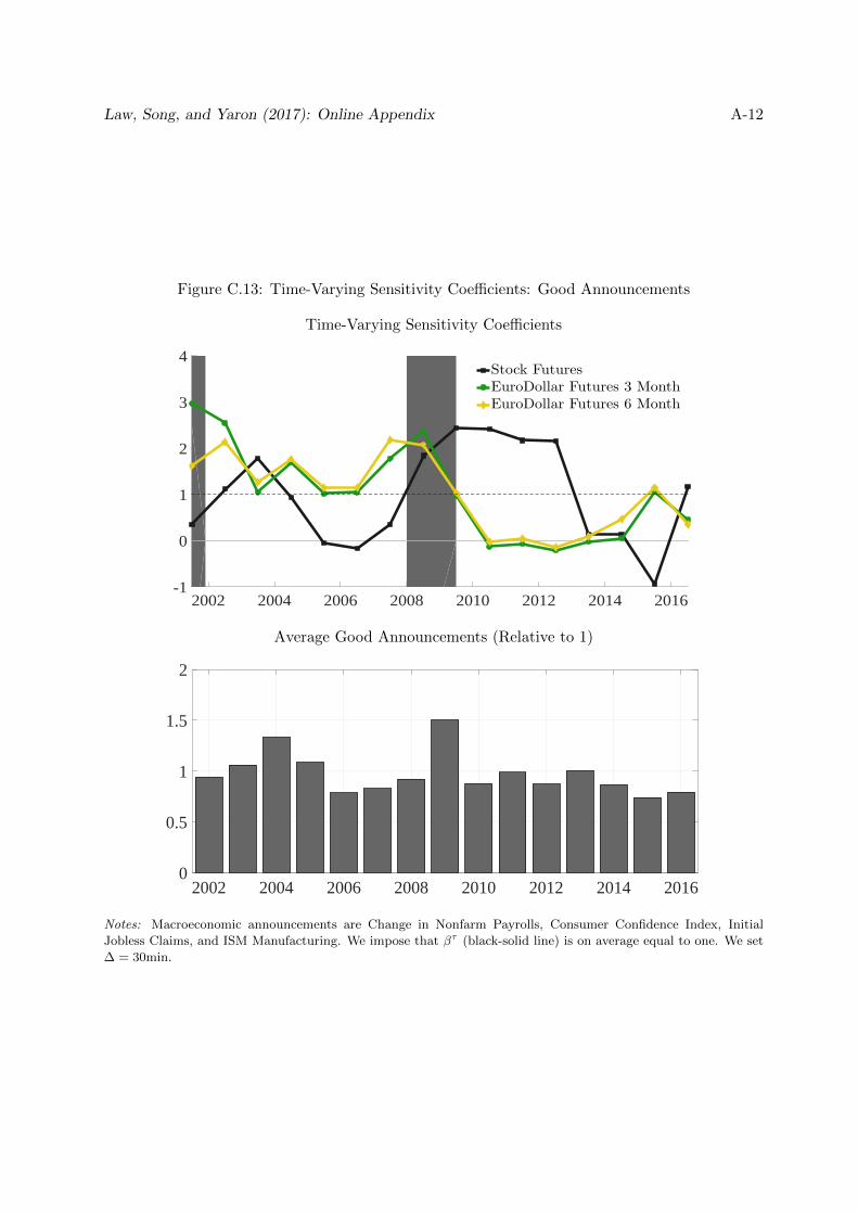
Law, Song, and Yaron (2017): Online Appendix A-12
Figure C.13: Time-Varying Sensitivity Coefficients: Good Announcements
Time-Varying Sensitivity Coefficients
2002 2004 2006 2008 2010 2012 2014 2016-1
0
1
2
3
4Stock FuturesEuroDollar Futures 3 MonthEuroDollar Futures 6 Month
Average Good Announcements (Relative to 1)
2002 2004 2006 2008 2010 2012 2014 20160
0.5
1
1.5
2
Notes: Macroeconomic announcements are Change in Nonfarm Payrolls, Consumer Confidence Index, Initial
Jobless Claims, and ISM Manufacturing. We impose that βτ (black-solid line) is on average equal to one. We set
∆ = 30min.
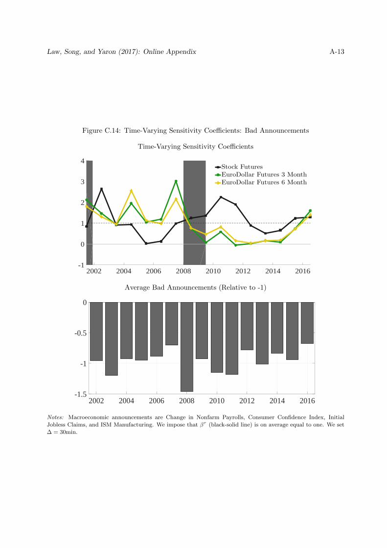
Law, Song, and Yaron (2017): Online Appendix A-13
Figure C.14: Time-Varying Sensitivity Coefficients: Bad Announcements
Time-Varying Sensitivity Coefficients
2002 2004 2006 2008 2010 2012 2014 2016-1
0
1
2
3
4Stock FuturesEuroDollar Futures 3 MonthEuroDollar Futures 6 Month
Average Bad Announcements (Relative to -1)
2002 2004 2006 2008 2010 2012 2014 2016-1.5
-1
-0.5
0
Notes: Macroeconomic announcements are Change in Nonfarm Payrolls, Consumer Confidence Index, Initial
Jobless Claims, and ISM Manufacturing. We impose that βτ (black-solid line) is on average equal to one. We set
∆ = 30min.
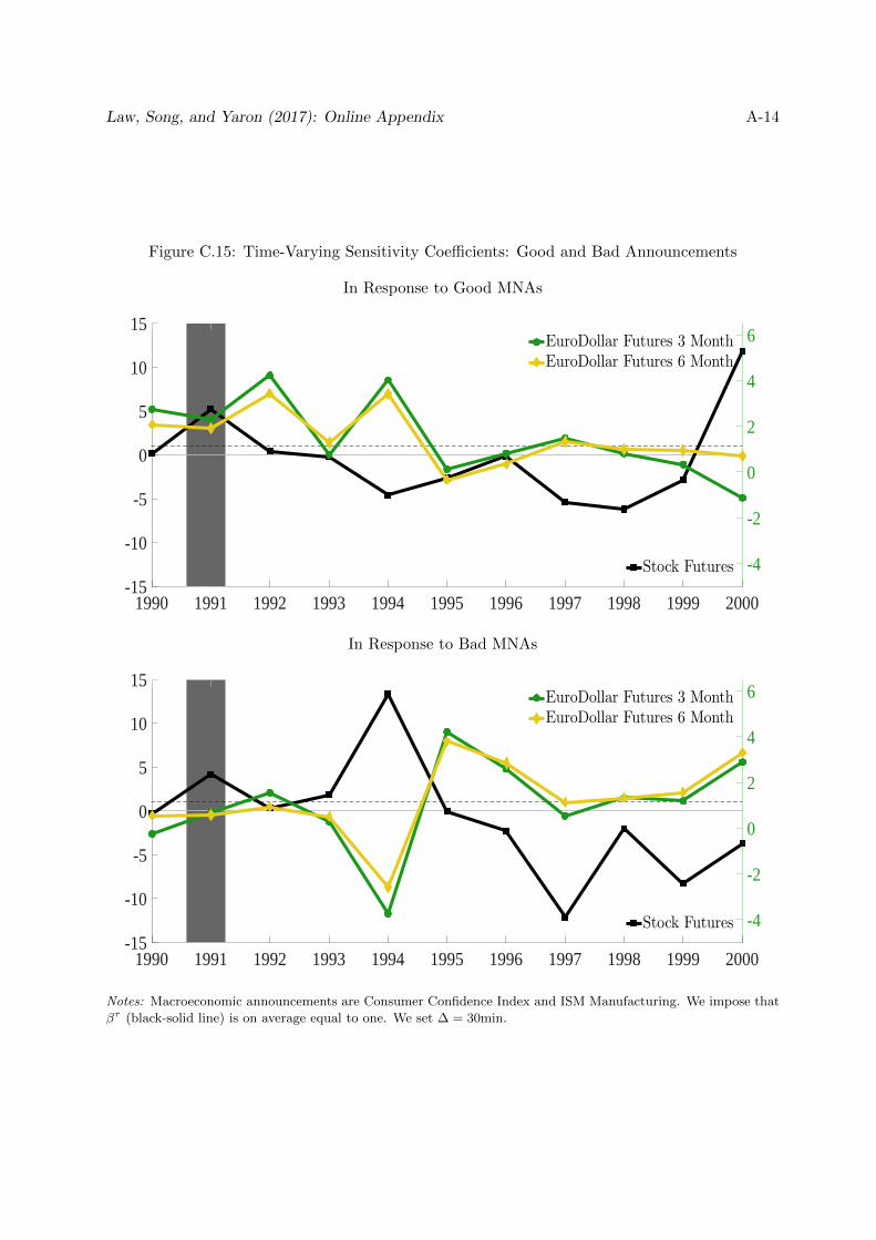
Law, Song, and Yaron (2017): Online Appendix A-14
Figure C.15: Time-Varying Sensitivity Coefficients: Good and Bad Announcements
In Response to Good MNAs
1990 1991 1992 1993 1994 1995 1996 1997 1998 1999 2000-15
-10
-5
0
5
10
15
Stock Futures
1990 1991 1992 1993 1994 1995 1996 1997 1998 1999 2000
-4
-2
0
2
4
6EuroDollar Futures 3 MonthEuroDollar Futures 6 Month
In Response to Bad MNAs
1990 1991 1992 1993 1994 1995 1996 1997 1998 1999 2000-15
-10
-5
0
5
10
15
Stock Futures
1990 1991 1992 1993 1994 1995 1996 1997 1998 1999 2000
-4
-2
0
2
4
6EuroDollar Futures 3 MonthEuroDollar Futures 6 Month
Notes: Macroeconomic announcements are Consumer Confidence Index and ISM Manufacturing. We impose that
βτ (black-solid line) is on average equal to one. We set ∆ = 30min.

Law, Song, and Yaron (2017): Online Appendix A-15
D News Decomposition under the Regime-Switching Model
Let St denote the regime indicator variable, St ∈ 1, 2. Define a Markov transition probability
matrix by Π
Π =
[p11 1− p22
1− p11 p22
]
which summarizes all 22 transition probabilities.
D.1 k Step ahead Expectations
Any variable Kt+1 that can be expressed as
Kt+1 = Λ0(St+1) + Λ1(St+1)Xt+1
Xt+1 = Φ(St+1)Xt + Ω(St+1)Σx(St+1)ηx,t+1, ηx,t ∼ N(0, I)
has the following k-step-ahead expectation form of
E(Kt+k|St) = E(Λ0(St+k)|St)︸ ︷︷ ︸Λ
(k)0
+E(Λ1(St+k)Φ(St+k)Φ(St+k−1) . . .Φ(St+1)|St)︸ ︷︷ ︸Λ
(k)1
Xt (A.1)
Kt+k = Λ0(St+k) + Λ1(St+k)Φ(St+k)Φ(St+k−1) . . .Φ(St+1)Xt
+ Λ1(St+k)Ω(St+1)Σx(St+1)ηx,t+k
+k−2∑i=0
Λ1(St+k)i∏
j=0
Φ(St+k−j)Ω(St+k−i−1)Σx(St+k−i−1)ηx,t+k−i−1.
We can characterize the constant and the slope coefficients as
Λ(k)0 (j) =
[Λ0(1) Λ0(2)
] [ p11 p12
p21 p22
](k−1)
×
[p1j
p2j
],
Λ(k)1 (j) =
[Λ1(1) Λ1(2)
] [ p11Φ(1) p12Φ(1)
p21Φ(2) p22Φ(2)
](k−1)
×
[Φ(1) 0
0 Φ(2)
][p1jI2
p2jI2
].

Law, Song, and Yaron (2017): Online Appendix A-16
The cumulative k-step-ahead expectation is
k−1∑i=0
E(Kt+i|St = j) =
(Λ
(0)0 (j) + Λ
(1)0 (j) + . . .+ Λ
(k−1)0 (j)
)(A.2)
+
(Λ
(0)1 (j) + Λ
(1)1 (j) + . . .+ Λ
(k−1)1 (j)
)Xt.
D.2 News and Shock Decomposition
For illustrative purposes, we assume that St−1 = m and St = j.
N(k)K,t = Et
( k∑i=1
Kt+i
)− Et−1
( k∑i=1
Kt+i
)(A.3)
= E
( k∑i=1
Kt+i|St = j
)− E
( k∑i=1
Kt+i|St−1 = m
)=
(Λ
(1)0 (j) + . . .+ Λ
(k)0 (j)
)+
(Λ
(1)1 (j) + . . .+ Λ
(k)1 (j)
)Xt
−(
Λ(2)0 (m) + . . .+ Λ
(k+1)0 (m)
)−(
Λ(2)1 (m) + . . .+ Λ
(k+1)1 (m)
)Xt−1
=
(Λ
(1)0 (j) + . . .+ Λ
(k)0 (j)
)+
(Λ
(1)1 (j) + . . .+ Λ
(k)1 (j)
)(Φ(j)Xt−1 + Ω(j)Σx(j)ηx,t
)−(
Λ(2)0 (m) + . . .+ Λ
(k+1)0 (m)
)−(
Λ(2)1 (m) + . . .+ Λ
(k+1)1 (m)
)Xt−1
=
(Λ
(1)0 (j) + . . .+ Λ
(k)0 (j)
)−(
Λ(2)0 (m) + . . .+ Λ
(k+1)0 (m)
)+
(Λ
(1)1 (j) + . . .+ Λ
(k)1 (j)
)Φ(j)Xt−1 −
(Λ
(2)1 (m) + . . .+ Λ
(k+1)1 (m)
)Xt−1
+
(Λ
(1)1 (j) + . . .+ Λ
(k)1 (j)
)Ω(j)Σx(j)ηx,t
=
(Λ
(1)0 (j)− Λ
(2)0 (m)
+ . . .+
Λ
(k)0 (j)− Λ
(k+1)0 (m)
)+
(Λ
(1)1 (j)Φ(j)− Λ
(2)1 (m)
+ . . .+
Λ
(k)1 (j)Φ(j)− Λ
(k+1)1 (m)
)Xt−1
+
(Λ
(1)1 (j) + . . .+ Λ
(k)1 (j)
)Ω(j)Σx(j)ηx,t

Law, Song, and Yaron (2017): Online Appendix A-17
denotes the news.
εK,t = Kt − E(Kt|St−1
)(A.4)
= Λ0(j) + Λ1(j)Xt − Λ(1)0 (m)− Λ
(1)1 (m)Xt−1
= Λ0(j) + Λ1(j)
(Φ(j)Xt−1 + Ω(j)Σx(j)ηx,t
)− Λ
(1)0 (m)− Λ
(1)1 (m)Xt−1
=
(Λ0(j)− Λ
(1)0 (m)
)+
(Λ1(j)Φ(j)− Λ
(1)1 (m)
)Xt−1 + Λ1(j)Ω(j)Σx(j)ηx,t
denotes the shocks.
If St−1 = j and St = j, we can express N(k)K,t and εK,t by
N(k)K,t =
(Λ
(1)0 (j)− Λ
(2)0 (j)
+ . . .+
Λ
(k)0 (j)− Λ
(k+1)0 (j)
)(A.5)
+
(Λ
(1)1 (j)Φ(j)− Λ
(2)1 (j)
+ . . .+
Λ
(k)1 (j)Φ(j)− Λ
(k+1)1 (j)
)Xt−1
+
(Λ
(1)1 (j) + . . .+ Λ
(k)1 (j)
)Ω(j)Σx(j)ηx,t
≈(
Λ(1)1 (j) + . . .+ Λ
(k)1 (j)
)Ω(j)Σx(j)ηx,t,
εK,t =
(Λ0(j)− Λ
(1)0 (j)
)+
(Λ1(j)Φ(j)− Λ
(1)1 (j)
)Xt−1 + Λ1(j)Ω(j)Σx(j)ηx,t
≈ Λ1(j)Ω(j)Σx(j)ηx,t.
E Solution of the Asset Pricing Model
The solutions are
Ψk(i) = ΨFk (i)
(Λk(j) + Φkk(j)pjiΨ
Fk (j)
Λk(i)Λk(j)− pijpjiΦkk(i)Φkk(j)ΨFk (i)ΨF
k (j)
), i, j, k ∈ 1, 2.
For ease of understanding, we express the regime-switching coefficient, Ψk(i), as function of the
fixed-regime coefficient,
ΨF1 (i) =
1
(1 + λ(i)φ(i))− piiΦ11(i), ΨF
2 (i) =−λ(i)
(1 + λ(i)φ(i))− piiΦ22(i).
For illustration, we focus on the first coefficient. Aggressive monetary policy raises φ and de-
creases the impact of real endowment shocks on expected consumption growth. Greater persis-
tence amplifies the impact of real endowment shocks on expected consumption growth. When the
real endowment shock is serially uncorrelated Φ11 = 0, the solution collapses to its fixed-regime
Law, Song, and Yaron (2017): Online Appendix A-18
counterpart, Ψ1(i) = ΨF1 (i). The interpretation of the second coefficient, loading on monetary
policy shock, is analogous to the first case except that its sign is negative.
The key feature is that expectations of policy behavior in regime 2 affect the equilibrium in
regime 1 and vice versa. Denote the denominator
Dk = Λk(i)Λk(j)− pijpjiΦkk(i)Φkk(j)ΨFk (i)ΨF
k (j).
Dk reaches its upper bound whenever regimes are absorbing states pij = 0. For all values of
pij 6= 0, Dk scales up the coefficients relative to their fixed-regime counterparts. In the limiting
case pij = 1, Dk raises the variability of expected consumption growth to its maximum amount.
There are two distinct effects that real endowment shock has on expected consumption growth,
which are highlighted in the numerator. The first is the fixed-regime effect and real endowment
shock directly raises expected consumption growth by an amount inversely related to monetary
policy coefficient φ. The second effect is the expectations formation effect. The term pjiΨFk (j)
arises from the expectation that regime switch can happen, with pji the probability of changing
from regime i to regime j.19
19The intuition is from Davig and Leeper (2007).