1

FE 257 GIS LAB 1 Basic GIS Operations with ArcGIS Pro Calculating Stream Lengths and Watershed Areas ArcGIS Pro offers some advantages for novice users. The graphical user interface is similar to many Windows packages and lets people use the software without having to spend a great deal of time learning commands. The software can be a little intimidating at first since there are many options and not a lot of guidance being offered. This lab will help you to understand ArcGIS Pro fundamentals and how to examine spatial data. ArcGIS Pro is split into a set of modules by a single project file (*.aprx file). The most-used modules are Map (for geodata viewing), Catalog (for database management), and Geoprocessing (for geodata manipulation). The GUI (Graphical User Interface) for each module offers different options depending on the active module and whether any software extensions have been activated. We will work with Map and Geoprocessing in today’s exercise. We’ll use Map first to import files. To access Map, we’ll need to start ArcGIS Pro. Before we start ArcGIS Pro, let’s copy some GIS data to your user workspace. Open the Windows Explorer and navigate to the t:\teach\classes\fe257\gislab1 location on the forestry network. Right click on this folder and choose Copy from the menu that appears. Next, navigate to a workspace on your computer that you have access to work in. Make sure this workspace is not “local” to your machine (e.g. the C drive) if you want to access your work on another machine outside of class time; instead, create a workspace on an OSU network drive (like your personal Z:\ or N:\ drive) and copy-paste your work to a local drive or USB to back it up – this is good data management practice. Create a subfolder named ‘fe257’ under your workspace folder – we’ll store and work with all the files from this course under that location, so make sure it is a good one! You can create the fe257 subfolder by clicking once on your workspace, choosing the File menu, the New option, and the Folder option. In the example screen below, I’ve chosen to save my work to the local C drive because I will be using this machine in the future; you may not have this convenience, so follow the instructions mentioned above to create a folder on an OSU network drive. I’ve created the fe257 folder under another folder called “khnic.” Once you’ve created the fe257 folder, copy the gislab1 folder from our course website to your fe257 folder. This should copy the gislab1 folder and included files into your new workspace.

2

Shapefiles The gislab1 folder contains four “shapefiles” compatible with ArcGIS Pro. The shapefiles contain vector layers (points, lines, polygons) representing geospatial information like city points, stream networks, and watershed areas. Since shapefiles are compatible with ArcGIS Pro, the program reads the files as geospatial data layers. Therefore, when viewing a shapefile in Catalog (remember, the database management module), the layer appears as a single file with a “.shp” extension.

However, things become more complicated when viewing shapefiles in Windows Explorer because they are not compatible with this program. In Explorer you’ll see nested files comprising the shapefile. Each file has a different extension type, including .shp but also including .dbf, .prj, and others.

This is because each of the nested files contains different geospatial information necessary for reading the shapefile. For example, the .prj file contains the map projection information and the .dbf file contains the tabular data associated with the shapefile. We will learn more about map projections and tabular data later! The important point of all this is: you can use Catalog to unworriedly move or copy-paste shapefiles with the single .shp extension. However, if you need to move or copy-paste a shapefile using Windows Explorer, you must include ALL the nested files and not just the .shp file. Otherwise, your shapefile will become corrupted and unreadable. Understanding how shapefiles work is critical to your knowledge of GIS. Map This is the central portion of ArcGIS Pro and is where we look at data and create maps. Let’s start a Map session by clicking the start menu or using the task bar search option to find the ArcGIS Pro executable. The start menu sequence is start button, ArcGIS, ArcGIS Pro and choosing the ArcGIS Pro icon.

3

The Project menu will open. Using ArcGIS Pro normally requires a monetary license, but OSU students can access the software for free through an Enterprise login. In the upper right-hand corner of your new project, you will see a sign in notification. Click “Sign in.”

You will then be prompted with the screen below. In “Your ArcGIS organization’s URL,” type “OSUGISci” and check the “Remember this URL” and “Sign me in automatically” options, then click Continue.

Your screen will change to the one below. Click on “Oregon State University.”

4

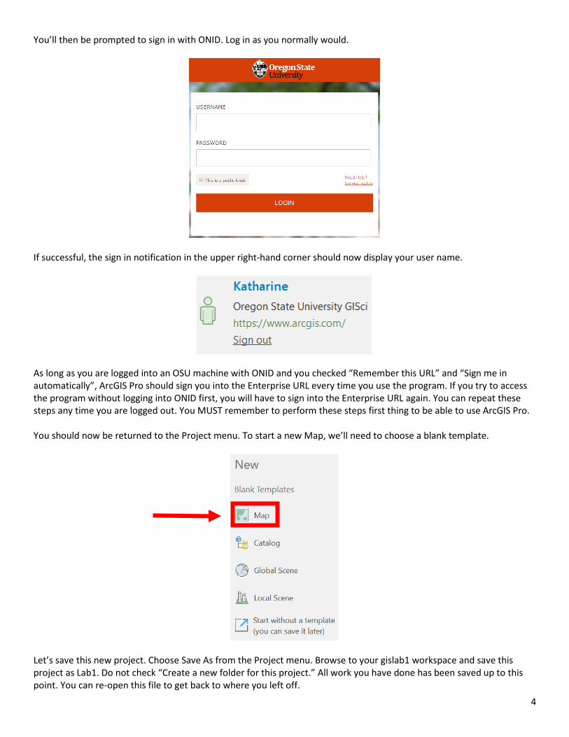
You’ll then be prompted to sign in with ONID. Log in as you normally would.

If successful, the sign in notification in the upper right-hand corner should now display your user name.

As long as you are logged into an OSU machine with ONID and you checked “Remember this URL” and “Sign me in automatically”, ArcGIS Pro should sign you into the Enterprise URL every time you use the program. If you try to access the program without logging into ONID first, you will have to sign into the Enterprise URL again. You can repeat these steps any time you are logged out. You MUST remember to perform these steps first thing to be able to use ArcGIS Pro. You should now be returned to the Project menu. To start a new Map, we’ll need to choose a blank template.

Let’s save this new project. Choose Save As from the Project menu. Browse to your gislab1 workspace and save this project as Lab1. Do not check “Create a new folder for this project.” All work you have done has been saved up to this point. You can re-open this file to get back to where you left off.

5

Your Map window should now open. Confirm that the top of your ArcGIS Pro window displays the saved project name and shows you logged in to the Enterprise URL. Save your project as often as possible! You will have to repeat a lot of steps if you do not save often and the program crashes on you, which you are likely to experience at some point.

At the top of the Map interface, you’ll see a row of menus, followed by a row of graphical buttons. On the left is the Contents window which lists each data file in your project. On the right are two windows you can toggle between: Catalog, which is the ArcGIS Pro version of Windows Explorer for organizing databases, and Geoprocessing, which includes tools and toolboxes to analyze and automate GIS data and tasks.

6

7

Importing Files

ArcGIS Pro will import and read shapefiles. This is important as many organizations that make spatial data available over the Internet or for purchase convert their data into shapefiles. As mentioned earlier, shapefiles are actually a collection of files. Exported shapefiles will have a .shp suffix attached to them.

To import a new file, you must first connect to the Windows folder containing that file through ArcGIS Pro. Select the Insert menu and click the Add Folder button.

Navigate to the workspace where you established your gislab1 folder and select it. Do not enter the folder, only select it.

If successful, the folder should appear in your Catalog window to the right.

8

Now that you’ve established a connection to the gislab1 folder, you can add data from that folder to your project. Return to the Map menu and click the Add Data button.

With a successful folder connection you should be able to select Folders > gislab1. Select the four shapefiles present in the gislab1 folder and click OK.

The four shapefiles should now appear in your Contents window. Notice how each vector type is represented visually in the Contents window: cities is a point layer, rivers and oregon are line layers, and wsheds is a polygon layer. The World Topographic Map is the base layer map that automatically appears when you open the Map window; you can turn this layer on and off depending if you want to view it alongside your layers or use it for mapmaking.

9

ArcGIS Pro allows us to manipulate the display of spatial data and perform basic analyses. Anytime you add data into Map, you are adding it to a data frame. You can have multiple datasets open at the same time in a frame and each data set is referred to as a layer. The names of data frames and layers and access to how you display each layer are in the Contents and Map windows. ArcGIS Pro has powerful features for controlling how points, lines, and polygons are displayed. You may have multiple data frames in ArcGIS Pro. The default name for each data frame is “Map,” but you can rename a data frame by right clicking on the default name, selecting Properties, and typing in the Name box.

The last operations should have opened all four shapefile layers into Map. In ArcGIS Pro terminology, each these shapefiles are now known as “layers” and are contained in the Map data frame. By default, ArcGIS Pro makes each of the layers visible. To make a layer not visible, just uncheck the check box located to the left of each layer name in the Contents. You should see all four imported layers in the Map extent, shown below.

Manipulating Layers

An important concept in ArcGIS Pro is the notion of the active data frame. If you have multiple data frames in the Contents and Map viewer, any operations you invoke will only consider the active data frame. You can make a data frame active by toggling between data frame windows in the Map viewer. The active data frame will appear in the Contents window. Layers are generally made active and accessed one at a time for display manipulations, but it is possible to have multiple active layers by clicking and holding the control key down. This may be useful for copy or deleting several layers at once. Active layers are indicated by highlighting in the Contents. It is also possible to copy and paste layers between different data frames; this skill may help you during course exercises. You can also assign a name to an active layer by double clicking or right clicking on the layer name, making the General tab active, and typing a name in the Name box. This new name will now appear in the Contents.

If multiple layers exist, the order in which layers appear in the Contents is also important. The layer on the bottom of the “stack” will be the first layer that is displayed in the view. A polygon layer that sits atop the stack may preclude all other layers from being displayed. You can move layers in the Contents by clicking on the layer, holding the mouse button down, and dragging it up or down. When imported, wsheds is at the bottom of the stack and all other layers are drawn on top of wsheds. Let’s see what happens when we move wsheds to the top of the stack.

10

Let’s move it back to the bottom of the stack.

“Wsheds” is an unusual name. Let’s change the name of the layer as it appears in the Contents by activating its Properties and typing “Watersheds” in the Name input box and choosing OK. Notice that the layer name has changed.

When you open multiple layers at the same time into a view, ArcGIS Pro will automatically adjust to the full geographic extent of all layers so that you are able to see all areas. This may be helpful in some cases but for today’s example, we are really only interested in the northwestern corner of Oregon. ArcGIS Pro features a tool bar that allows us to interact with data frames and layers.

ArcGIS Pro has several options for zooming in and out of the map display area. Let’s use the zoom in tool to focus on our study area. Select the zoom in tool by clicking on it with your mouse. You can also zoom using your mouse’s scroll wheel.

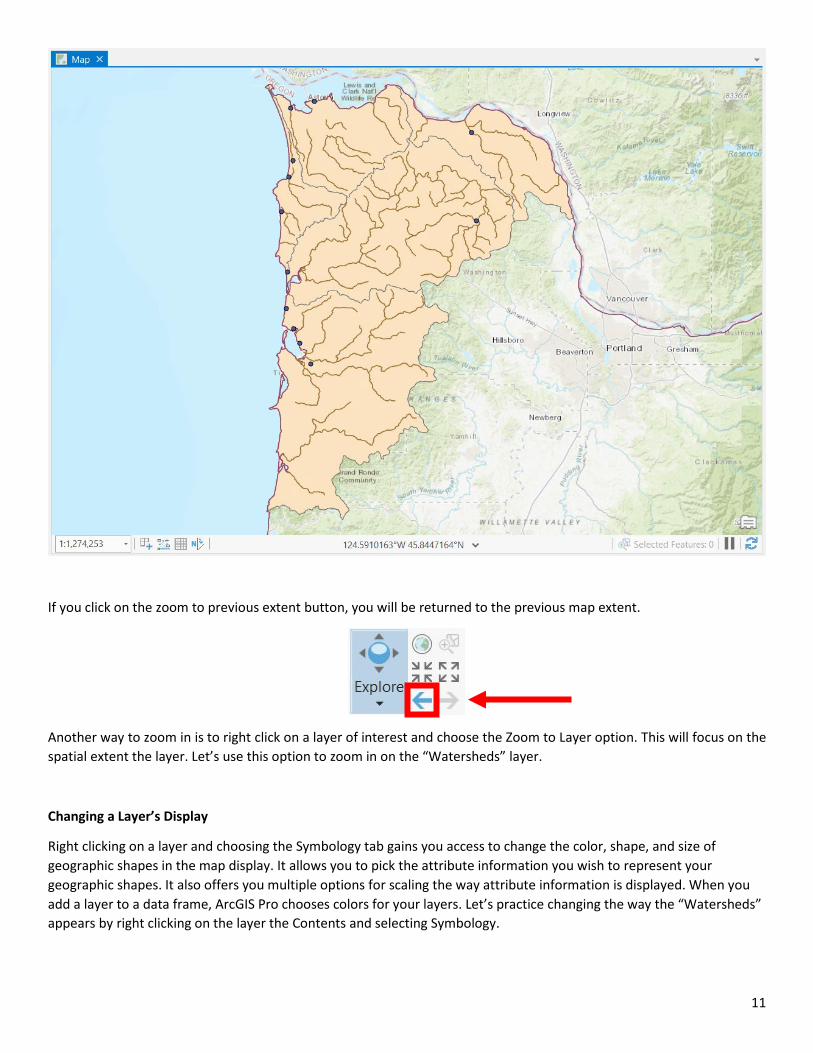
You can click the zoom in button and use your panning cursor (the hand cursor) to zoom into northwest Oregon, your area of interest. Your new perspective should look similar to the figure below.

11

If you click on the zoom to previous extent button, you will be returned to the previous map extent.

Another way to zoom in is to right click on a layer of interest and choose the Zoom to Layer option. This will focus on the spatial extent the layer. Let’s use this option to zoom in on the “Watersheds” layer.

Changing a Layer’s Display

Right clicking on a layer and choosing the Symbology tab gains you access to change the color, shape, and size of geographic shapes in the map display. It allows you to pick the attribute information you wish to represent your geographic shapes. It also offers you multiple options for scaling the way attribute information is displayed. When you add a layer to a data frame, ArcGIS Pro chooses colors for your layers. Let’s practice changing the way the “Watersheds” appears by right clicking on the layer the Contents and selecting Symbology.

12

A new window will appear on the right displaying primary symbology with Single Symbol selected in the drop-down menu. Click on the colored box next to Symbol to open up the Gallery. This will produce pre-made colors representing certain infrastructure and land use types, but you can assign any of these colors to your shapefiles regardless of the data type. The other option is to select Properties and manually assign a color and/or outline as you would in any other Windows program, then click Apply. Pick a color with a light shade.

13

We can also use the Symbology interface to color code a layer based on a variable within the layer’s attribute table. Change the primary symbology drop-down menu to Unique Values. Use the drop-down menu next to the Field 1 line and choose HUC (Hydrologic Unit Code) from the list of variables. Do you notice any changes in your map regarding the way the layer is displayed? This creates a color identity for each of the five watersheds based on their unique HUC code.

Let’s revert to a single layer color by returning to primary symbology, selecting Single Symbol and changing the color using Gallery or Properties.

Let’s follow the same process for the rivers layer so that a nice deep blue represents the rivers. You may want to adjust the width of the lines to make viewing easier. We may also want to change the name as it appears in the Contents to Rivers.

14

The pan tool is very useful for moving around in your view. This is the cursor that looks like a pointing hand and is the default Map cursor. You can also use this cursor to select and identify objects. Use the Explore tool to access the pan and identify options. Below is a list of mouse capabilities using the Explore tool.

Place the pan cursor in the middle of your viewing area and click and drag the mouse. Notice that your viewing area moves as you move the mouse. Releasing the mouse button will place the view.

Another very useful tool is the left-click identification tool. We will use this and an automatic labeling option under the layer menu.

15

Change the name of the “cities” point layer to Cities. Use the left-click identification tool to click on one of the point locations associated with the Cities layer. A table should appear containing all the data associated with that point location. Notice that you can click on other points and the information in the table will change to reflect those points.

Let’s change the symbology of the Cities layer so that it stands out more.

Let’s experiment with labeling map features. You can create labels using a simple or more complex method depending on whether the default labeling settings work for you. The simple method involves right clicking on the Cities layer and choosing Label from the pop-up menu. We can turn this feature off by clicking on Label again. The complex method allows the user to customize which variable the labels display. In this case, we want to display city names. Similar to the simple method, right click on the layer, but this time choose Labeling Properties to open the label class window.

16

Label Class allows the user to build an expression displaying the variable of interest. The default expression is “$feature.NAME”, but let’s see how this was created. Delete the default expression and scroll to NAME under the Fields menu, then double click. You are telling the program to create an expression for labeling cities based on their name variable. You can also toggle to Symbol or Position at the top of the Label Class menu to format the labels’ appearance and modify their position around features if the labels are blocking features you wish to display. Click Apply when you are satisfied with your expression and formatting, and you should see something like the screenshot below.

Attribute Data

Attribute data are the data associated with layers. It’s relatively easy to access this information in ArcGIS Pro and we can edit, summarize, and export attribute data. ArcGIS Pro will also allow you to import database files from other GIS packages, dBase files, and even from text files. You can also export data into these same formats. You may have multiple tables in a project. You can open a layer’s attribute data by right clicking on the layer and choosing Attribute Table from the pop-up menu.

Once attribute data are displayed, they can be easily edited. ArcGIS Pro will also allow you to add and delete variables. Character variables must be created as a string type. You can use the field calculator to perform calculations on entire database or on portions of it.

Make “Watersheds” the active layer and open its attribute table using the method described above. Notice that data are displayed for each of the five polygon records contained in the layer.

17

The area measurements are in square international feet. Let’s add a new variable that describes the size of each watershed as a percentage of all five watersheds. First, select the icon in the upper left-hand corner of the attribute table, then choose Add Field.

Enter Pct_Area in the name box, make sure type is set to Short integer, and enter 4 in the precision box.

Then click Save in the Fields toolbar. Once saved, the program populates the rest of the columns.

18

Before we can calculate watershed percent areas, we need to know the sum of the watershed areas. Right click on the AREA field heading and choose Statistics. The number we want is the sum: 71391653888.

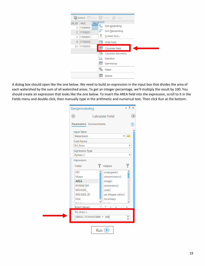
Let’s finish our calculations by right clicking the top of the Pct_Area variable and selecting the Calculate Field choice.

19

A dialog box should open like the one below. We need to build an expression in the input box that divides the area of each watershed by the sum of all watershed areas. To get an integer percentage, we’ll multiply the result by 100. You should create an expression that looks like the one below. To insert the AREA field into the expression, scroll to it in the Fields menu and double click, then manually type in the arithmetic and numerical text. Then click Run at the bottom.

20

Now when you view the Pct_Area field, each of the five watersheds will have a percent area calculation. Look at the size of each watershed in your Map viewer to confirm that these calculations generally make sense.

We can sort attributes by right clicking on the field heading of interest and choosing Sort Ascending or Sort Descending from the pop-up menu. Let’s experiment a little with this. You can also select records and see their locations in the map display area highlighted in bright blue. Let’s try this option also. We should also check our results by performing the Statistics option on the Pct_Area field; this should sum to 100 or something very close.

Notice that you can hold down the control or shift keys and make multiple record selections. When a record(s) is selected you can unselect it by choosing Clear Selection from the table toolbar. Notice your other selection choices too.

Let’s clean up our work by making the Pct_Area field active by right clicking on its top and choosing Delete Field from the pop-up menu. Let’s close this table.

Let’s explore some additional attribute table options by going to the Rivers layer and opening its attribute table. One of the tools we have in the attribute portion is the ability to summarize a variable. Let’s test how this works.

1. Scroll to the right to find the variable titled “PNAME” and make it active by right clicking on its top. “PNAME” is the name of each river in the Rivers layer.

2. From the pop-up menu choose Summarize and OK.

21

3. A summarize dialog box should open up. The input table should be Rivers. Direct the output to your gislab1 folder by using the browse button. Under Statistics Field(s), select PNAME for Field and Count for Statistic Type. Click Run.

4. This should create and add to your ArcGIS Pro session (in the Contents) another attribute table that shows the number or arcs, or line segments, that are associated with each unique occurrence of “PNAME.” Right click on the table and choose Open.

22

This process created a field summarizing how many line segments in the Rivers layer share the same name. Multiple line segments share the same name because of processes that occurred during digitization of the river network for GIS use. The computer program or GIS professional tasked with digitizing the River layer may have created multiple line features for one singular river. For example, in the table above, Beaver Creek is made up of two line features and Clatskanie River is made up of three line features. This presents a problem when trying to make certain calculations like total length of a river. Without combining the collection of line features comprising a river, we will only be able to calculate the lengths of each river segment individually. This will produce incorrect values representing the length of one segment versus the length of the entire river. You can experiment with this yourself by calculating river lengths before and after the next steps in this lab on pages 23-24. Notice how Frequency and Count produce the same numbers, because count is the same concept as frequency.

If we want more than just a frequency distribution, we’ll need to modify what we enter in the summarize box. Let’s find out which river is the longest. Close the output table we just created and go back to the attribute table for Rivers (you may need to re-open it from the Contents).

1. Right click on PNAME and choose the Summarize tool.

2. A summarize dialog box should open up. The input table should be Rivers. Direct the output to your gislab1 folder by using the browse button. Under Statistics Field(s), select LENGTH for Field and Sum for Statistic Type. Click Run.

23

Open the resulting table in the Contents by right clicking on it and choosing Open. The output table lists each river’s record number, name, number of arcs, and total length. Right click on the SUM_LENGTH field header and select “Sort Ascending” or “Sort Descending” to identify the longest or shortest river.

Let’s close these output tables and return to the Map display area.

Let’s rename our data frame by right clicking on “Map” and selecting Properties, or simply double clicking. Enter the name “Watershed Area” into the Name box. You will see the name change in the Contents window.

Choose OK to make the change take effect.

24

In the next lab, we’ll create a set of maps for our watersheds and their locations. We will need to create multiple data frames to accomplish this. Let’s create a new data frame that will hold only the Oregon outline and the watershed polygons. Rename the state outline layer to “Oregon” if you have not done so already. From the Insert menu, choose New Map.

Note that a new data frame called Map1 will appear in your Map viewer and activating it will switch the Contents window to the layer stack contained in that data frame. If your Map1 appeared in a new viewing window, drag and dock the Map1 tab into the same viewing window as the Watershed Area map. You should now see two tabs at the top. You can toggle back and forth between them, noticing the Contents change simultaneously.

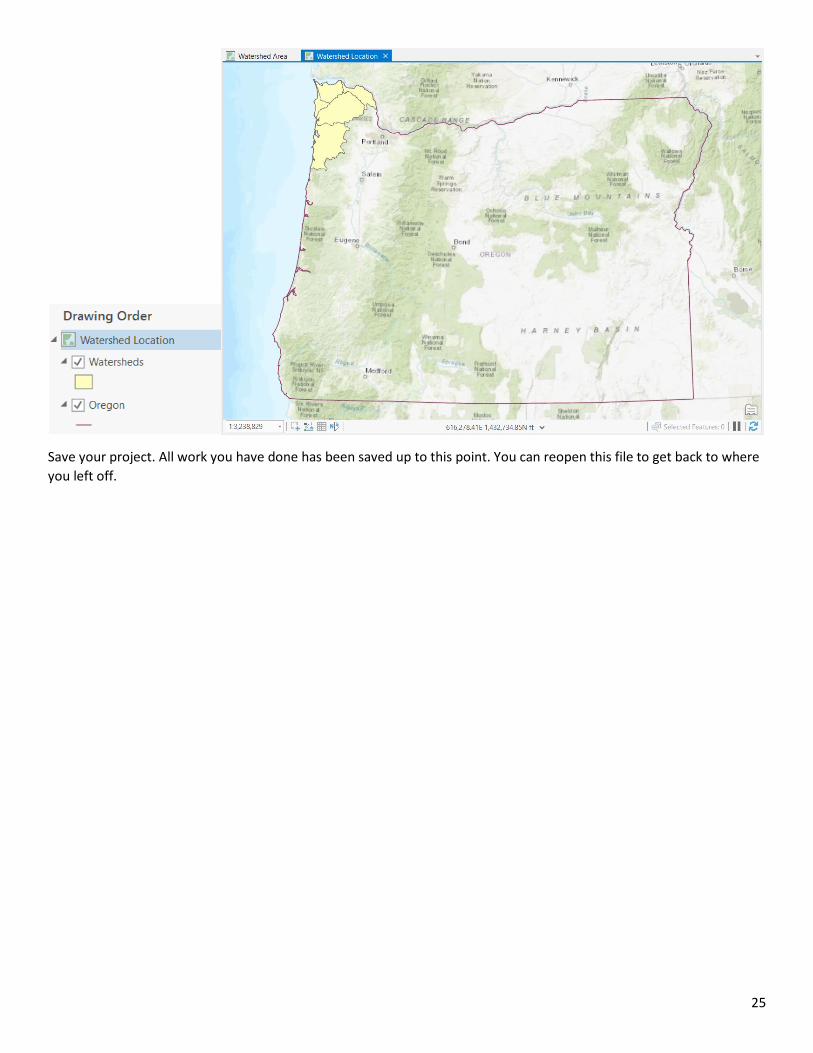
Let’s right click on the Oregon layer in your Watershed Area data frame and choose Copy from the pop-up menu. Right click on the new Map1 data frame in the Contents and choose Paste. Let’s repeat this process for the Watersheds layer. When finished pasting, remove the Oregon layer from the Watershed Area data frame by right clicking on it and choosing Remove. Let’s also rename the new data frame to Watershed Location. When Watershed Location is activated your Contents and Map viewer should look like the screenshot below. Use the Full Extent button to refresh the display.

25

Save your project. All work you have done has been saved up to this point. You can reopen this file to get back to where you left off.

26

LAB 1 Application: Calculating Stream Lengths and Watershed Areas. Assignment 1. Please answer the following questions and present your type written answers by the start of your lab during week 2. Be sure to include your name, course number (FE 257), assignment number, and lab day and time (please include both so we can keep track of your assignments) in the upper left-hand corner of the first page. 1A. We worked with several databases during the lab assignment in class. Two of the layers we examined were a watershed and a river coverage from Oregon's coast. Once you complete the lab assignment, you should have the skills to answer a few questions about the layers. Please answer the following (five points):

A. What is the relative size percentage by HUC number for the two most southern watersheds? You should create a table with two columns for your results. One column should contain the HUC number for each of you watersheds and the other column should contain the percent size. Each column should have a title.

Example: HUC Percent area

B. What are the names of the third shortest and third longest rivers/creeks in the Rivers layer?

C. What is the name of the city located farthest to the north? 1B. GIS concepts and definitions were presented during the first lecture and in Chapter 1 of your book. On pages 24-25 of the course text, please answer the following questions:

1.5 – List one pioneer and briefly describe their accomplishments (two points)

1.11 – List three techniques- you don’t need to describe them (three points) Please read chapter 1 for this week, and chapters 2 and 4 (read chapter 4 before chapter 2 to prepare for the week 2 lab) in your text book in preparation for next week.