1

FastMag: Fast micromagnetic simulator for complex magnetic structures

R. Chang, S. Li, M. V. Lubarda, B. Livshitz, and V. Lomakin

Center for Magnetic Recording Research and Department of Electrical and Computer

Engineering, University of California, San Diego

Abstract

A fast micromagnetic simulator (FastMag) for general problems is presented. FastMag solves the

Landau-Lifshitz-Gilbert equation and can handle problems of a small or very large size with a

high speed. The simulator derives its high performance from efficient methods for evaluating the

effective field and from implementations on massively parallel Graphics Processing Unit (GPU)

architectures. FastMag discretizes the computational domain into tetrahedral elements and

therefore is highly flexible for general problems. The magnetostatic field is computed via the

superposition principle for both volume and surface parts of the computational domain. This is

accomplished by implementing efficient quadrature rules and analytical integration for

overlapping elements in which the integral kernel is singular. Thus discretized superposition

integrals are computed using a non-uniform grid interpolation method, which evaluates the field

from N sources at N collocated observers in ( )O N operations. This approach allows handling

any uniform or non-uniform shapes, allows easily calculating the field outside the magnetized

domains, does not require solving linear system of equations, and requires little memory.

FastMag is implemented on GPUs with GPU-CPU speed-ups of two orders of magnitude.

Simulations are shown of a large array and a recording head fully discretized down to the

exchange length, with over a hundred million tetrahedral elements on an inexpensive desktop

computer.

2

1 Introduction

Micromagnetic solvers for the Landau-Lifshitz-Gilbert equation have a significant predictive

power and are important for our ability to analyze and design magnetic systems. Micromagnetic

simulations of complex structures, however, may be very time consuming and their acceleration

methods are of high importance. Currently available micromagnetic solvers are based on the

finite-difference method (FDM) [1-3] or finite element method (FEM) [4-6]. FDMs can be

efficient for problems of regular shapes discretized uniformly but they are less suited for general

problems with complex geometrical and material compositions. FEMs provide flexible tools for

micromagnetic simulations of complex general structures but their efficient implementations for

large-scale structures may be complicated.

Due to the speed saturation of single-core computing systems, modern and future computational

tools should rely on parallelization to allow for continued scaling of the computational power.

Several parallel implementations of FDMs and FEMs on CPU shared memory computers and

clusters exist [7-9]. However, current shared memory computers are limited in the number of

available cores while large clusters are expensive, consume much power, and are available only

as specialized facilities. New massively parallel Graphics Processing Unit (GPU) computer

architectures have emerged, offering massive parallelization at a low cost. A simple desktop with

a single GPU may offer the computational power matching or exceeding that of a CPU cluster

but at a fraction of its cost. Multiple-GPU parallelization can lead to further significant

computational power increases. The use of GPUs has been recently demonstrated for FDM- and

FEM-based micromagnetic solvers with significant acceleration rates [10-12]. However, the

currently reported solvers have several limitations. The FDM solvers cannot easily handle

general geometries while FEM-based approaches do not parallelize the fast algorithm for the

magnetostatic field evaluation and may reduce their performance for large problems due to the

need to solve linear systems at each time step.

3

In this paper, we present a fast micromagnetic simulator, referred to as FastMag, that can handle

problems of a small or very large size with a high speed. FastMag discretizes the computational

domain into tetrahedral elements and, therefore, is highly flexible for problems of any geometry

and material composition. The differential operators are implemented in an FEM-like manner.

The magnetostatic field is computed via the superposition principle for both volume and surface

parts of the computational domain. The superposition integrals are discretized using an efficient

approach and are computed via the non-uniform grid interpolation method (NGIM) in ( )VO N

operations for a problem with VN degrees of freedom (e.g. mesh nodes) [10, 13-15]. FastMag

has advantages of both FDM and FEM and offers additional benefits. It allows handling any

uniform or non-uniform geometries, does not require solving a linear system of equations for

magnetostatics, and requires little memory. FastMag is implemented on CPUs and GPUs with

GPU-CPU speed-ups of two orders of magnitude, allowing for simulating structures meshed into

over a hundred million tetrahedrons on inexpensive desktop computer and it has a potential for

simulating much larger structure on larger computer systems. The efficiency of FastMag is

demonstrated by simulating a large array of magnetic elements and a complex recording head

fully discretized with the mesh edge size of the exchange length. FastMag and its extensions can

be used to micromagnetically model general magnetic structures, such as uniform and non-

uniform arrays of generally shapes magnetic dots, recording heads, and magnetic media, among

others.

The paper is organized as follows. Section 2 formulates the problem. Section 3 presents the

discretized formulation. Section 4 describes how the effective fields are computed. Section 5

discusses aspects of the code implementation on GPUs. Section 6 demonstrates the code

performance via numerical results. Section 7 summarizes findings of the paper.

2 Problem formulation

Micromagnetic phenomena are governed by the Landau-Lifshitz-Gilbert (LLG) equation, which

assumes that the magnetization is a temporally and spatially continuous function. The LLG

equation can be written as

4

eff eff2( )

1 st M

MM H M M H , (1)

where M is the magnetization vector, sM is the saturation magnetization, t is time, is the

gyromagnetic ratio, and is the damping constant.

The effective magnetic field effH in Eq. (1) is comprised of the external field extH , anisotropy

field aniH , exchange field excH , and magnetostatic field msH , which are given (assuming the

CGS system) by

eff ext ani exc s

2

m

2

'.

( )

2

Ka

m

ni

s

exc

s

s

V S

H

M

A

dV dS

M

H H H H H

n

r r

H k M k

H M

r

M

r

MH

(2)

Here, the anisotropy field is assumed to be uniaxial, KH is the anisotropy field, A is the

exchange constant, and the external field is a prescribed function of space and time. The

magnetostatic field is given as a volume integral over the effective volume charges M and

surface integral over the effective surface charges M n defined with respect to the normal to

the computational domain surface n . The superposition approach in Eq. (2) allows computing

the magnetostatic field without a need for an iterative solver, which is an advantage over

conventional FEM micromagnetic solvers. However, the evaluation of the magnetostatic field as

in Eq. (2) may be slow unless it is implemented using fast techniques. An implementation of

such a technique is presented in Sec. 4.

3 Magnetization representation

To solve the LLG equation accurately the magnetic structure of interest is discretized into a mesh

of tetrahedrons. Tetrahedral elements are preferred over other elements, e.g. rectangular or prism

5

elements, because of their ability to accurately represent structures of arbitrary shape and aspect

ratio. Several types of basis functions can be used to represent the fields. For example SWG

basis functions used for electromagnetic integral equations can be used [16]. In this work we use

standard scalar linear basis functions defined on the tetrahedral elements. This approach makes

various parts of the developed codes compatible with other existing micromagnetic codes.

Let the total number of tetrahedral elements be TN , the total number of nodes (i.e. tetrahedron’s

vertices) be VN , and the number of surface triangles be SN . Let the nodes, volume elements,

and surface triangles be numbered, e.g. by a mesher. Assume that the volume connectivity table

( , )VC e i is available that defines the volume elements e in terms of node numbers i , with 4

nodes per element. Assume that the surface connectivity table ( , )SC e i is available that defines

the surface triangles in terms of the node number i , with 3 nodes per triangle. Assume also that

the magnetization is defined at the nodes, with the total 3 VN degrees of freedom. The

magnetization vector at a location r in space can be represented in the following form

4

( , ) ,

1 1

( ) ( )T

V

N

C e i e i

e i

M Mr r . (3)

Here, the summation represents the magnetization at each element e in terms of interpolation

function ,e i corresponding to the node i of the element e , weighted with the magnetization

vector at this node. The interpolation function is non-vanishing in the domain of the element

only, is unity at the node i of this element, and linearly tapers to zero at the element’s face

opposite to the node. Higher order interpolation functions can be chosen as well.

The expansion of the magnetization in Eq. (3) is substituted into the LLG equation (1), the

resulting effective field is computed at the nodes. Such computation can be considered as a

transformation from 3 VN magnetization states to 3 VN effective field states. An approach to

perform this transformation is discussed next.

6

4 Calculations of the effective field

4.1 Anisotropy, external, and exchange fields

Computing the external and anisotropy fields is straightforward. These fields are directly

sampled at the nodes and if required they can be calculated in space as in Eq. (3). The

computational cost associated with these operations is ( )VO N and is very low.

Computation of the exchange field can proceed as in conventional FEM/BEM methods. For

example, the exchange field can be computed via the box method, as outlined in Ref. [17]. Since

the exchange field is given by local differential operators, it can be represented in terms of sparse

matrix-vector products with a computational cost of ( )VO N .

4.2 Magnetostatic field

The magnetostatic field is computed directly as the spatial superposition in Eq. (2). This

approach, therefore, combines the generality of FEM/BEM and high speed of FDMs. Achieving

high accuracy using this approach requires developing methods for fast and accurate evaluation

of the superposition integrals on tetrahedral meshes. Approaches to accomplish this task are

described next.

4.2.1 Discretization

The use of the linear basis functions leads to constant charge densities in the tetrahedrons and

linear surface charge densities over the triangular surfaces. The volume and surface charge

densities can be written as

4

( , ) ,

11 1

3

( , ) ,

11 1

( ) ( ) ( ) ( ),

ˆ ˆ( ) ( ) ( ) ( ) ( ).

T T

V

S

S S

N N

C e i e i e

ie e

N N

e C e i e i e

ie e

q q

r rM M r r

r n r rM n rM

(4)

7

Here, the volume charge density 4

( , ) ,1( ) ( )

Ve C e i e iiq

rMr is a constant in the domain of the

volume of the element e and vanishes outside this domain (for the linear interpolation functions

used). The surface charge density 3

( , ) ,1ˆ( ) ( ) ( )

Se e C e i e ii

r n rM is a linear function in the

surface triangle e with the outward normal ˆen and it vanishes outside this triangle. The function

, ( )e i r is a surface interpolation function, which is non-vanishing in the domain of the surface

triangle e , is unity at the node i of this triangle, and linearly tapers to zero at the triangle’s side

opposite to the node. Higher order interpolation functions can be used as well.

The magnetostatic field is obtained similar to the framework of electromagnetic integral equation

solvers. The scalar potential ms

j is evaluated at the nodes (with coordinates jr ) via

11

( ) ( ).

T S

e e

N Nms ej

ee V Sj j

eqdV dS

r r

r r r r

(5)

where eV is the volume of the e -th tetrahedron and

eS is the surface of the e -th surface triangle.

Next, the potential in the entire domain is linearly interpolated from the nodal values as

4

( , ) ,

1 1

( ) ( )T

V

Nms

C e i e i

e i

ms

r r . (6)

The magnetostatic field is found via

4

( , ) ,

1 1 1

( ) ( ) ( )T T

V

N Nms ms

ms ms C e i e i e

e i e

rH rHr , (7)

where the fields ( )ms

eH r are magnetostatic fields that are constant over the domain of e -th

elements for the linear interpolation functions chosen. The value of the magnetostatic field at a

node is computed as the average of the fields in the surrounding tetrahedrons weighted by their

volumes.

8

A critical part in this procedure is evaluating the integrals in Eq. (5). In this paper, the integrals

are evaluated numerically using a quadrature rule and singularity extraction procedure similar to

the approaches used in the framework of electromagnetic integral equations [16]. The part of the

potential at a node generated by charges in its adjacent elements is computed analytically. All

other parts of the integrals are computed numerically via a quadrature rule [18]. We use a 4-point

rule in which the quadrature points coincide with the nodes (vertices) defining the tetrahedral

elements. Our numerical experiments demonstrate that such rules have a sufficiently high

accuracy while resulting in a significantly reduced computational cost as compared to rules with

quadrature points defined inside the element (see the discussion on accuracy in Sec. 6.1).

The entire procedure can be summarized in the following matrix form

0lms Z P ZH ZM QM . (8)

Here, M is a column vector of length 3 VN containing nodal magnetization components, Q is an

3V VN N matrix that projects the nodal magnetizations to the nodal point charges and the matrix

P is an 3 V VN N matrix that maps the nodal potentials to the nodal magnetostatic fields. The

matrix 0

Z is an V VN N matrix that describes the local corrections (singularity extractions) in

the potential. The matrices Q , P , and 0

Z are sparse and have nonvanishing entries only for

nodes that share the same tetrahedral element. The matrix l

Z is dense and it represents a

mapping from VN scalar charges to VN scalar observers with its entries given by

1 ;{ }

0;

ij

ijl

R i j

i j

Z

(9)

where ijR is the distance between the i -th and j -th node. This matrix represents the (long-range

interaction) integral kernel in a canonical (point-to-point) form.

The representation in Eq. (8) is efficient and flexible in that it decouples the basis function

representation from the integral kernel representation of the problem. In terms of the code

developments it allows easily switching between different types of basis and testing functions or

different types of the integral kernel. For example, SWG vector functions [19], edge elements

9

[20], or Voronoi tessellation can be used instead of the scalar hat function with the need to only

update the sparse matrices. Other types of integral kernels, e.g. periodic kernels or layered

substrate kernels [21], can be used without a need to change the rest of the code. The matrix [ ]lZ

is dense and the associated matrix-vector product has a computational cost of 2( )VO N if

evaluated as a direct summation. The following section describes how this product can be rapidly

evaluated in ( )VO N operations.

4.2.2 Non-uniform grid interpolation method for evaluating the dense interaction matrix

The multi-level NGIM divides the computational domain into a hierarchy of levels of boxes

similar to other multi-level algorithms. At each level (except the coarsest and the finest levels) a

box has one “parent” box and eight “child” boxes. This dividing process proceeds until boxes at

the finest level contain less than a prescribed number of sources. For a certain observation point,

boxes within a predefined distance are identified as the near-field boxes and are computed

directly. Other boxes farther than that distance are identified as the far-field boxes and are

computed via NGIM [10, 13-15].

NGIM saves the computational time by exploiting the fact that the static field/potential observed

outside a source domain varies slowly. This slowly varying field can be represented accurately

by samples at a highly sparse non-uniform grid (NG). Similarly, the field in a source-free domain

varies slowly. This field can also be sampled at a sparse Cartesian grid (CG) and interpolated to

the required observers. These interpolation operations are done in several stages of the multi-

level algorithm. Within each stage, the mathematical operations are independent with a small

overlapping of data, which makes massive parallelization possible.

The algorithm comprises five stages, including the near-field evaluation stage and four far-field

evaluation stages. In stage 1 of the far-field evaluation algorithm, NGs of boxes at the finest level

are constructed and the fields are evaluated on their NGs by direct superposition. In stage 2,

fields at NGs of higher level boxes are obtained via interpolation from their child boxes. In stage

3, field at CGs of boxes at all levels are evaluated by interpolating from NG samples at the same

10

level and the CGs of the corresponding parent boxes. Finally, in Stage 4, fields at the required

observers are obtained by interpolating from the CGs of the boxes at the finest level.

The computational time and memory of the algorithm scale as ( )VO N . NGIM can be applied to

uniform or non-uniform source-observer distributions. It can be automatically adaptive, e.g.

become faster, to reduced dimensionality geometries. It is also adaptive to sparse geometries, e.g.

geometries with empty spaces.

5 Implementation on Graphics Processing Units (GPUs)

The approaches discussed above are well suited to be implemented on GPUs. NVIDIA CUDA

programming environment provides a convenient framework for such implementations [22]. A

single GPU contains several hundred of stream processors, e.g. a recently released NVIDIA

GeForce GTX 480 has 480 stream processors (double number compared to the previous

generation). The processors are addressed via CUDA threads. The “atomic” thread unit is a

group of 32 threads, which is referred to as “warp”. A certain number of warps executing similar

operations can form a thread block. The blocks are given special privilege in utilizing fast shared

memory, which can be used efficiently as an intermediate storage. Most of the data is stored in

global memory. The maximal speed of the global memory is high (e.g. 177 GBits/sec bandwidth

for nVidia GeForce GTX 480), but it has a noticeable latency in handling every read or write

instruction (e.g., 400-500 cycles for nVidia GeForce GTX 480). This latency can be overcome

by a coalesced accessing scheme, where several reading or writing instructions are combined

within one transaction. This faster scheme is triggered when threads in the same warp access a

contiguous address. These features of the GPU architecture has to be carefully taken into account

when implementing the methods described above [14]. In particular, the NGIM implementation

on a CPU and a GPU has significant differences. Some of the key points allowing for efficient

GPU implementations of NGIM are summarized next.

1) A key feature in the GPU codes is the layout of data structure. To allow for the coalesced

accessing of the GPU global memory, all data belonging to a certain box is stored in

contiguous physical addresses. Special patterns of storage are adopted to make one copy

of source data, e.g. the arrays containing the coordinates and amplitudes of the

11

sources/observers are rearranged at all boxes at all levels. This leads to major

improvements as compared to more random data arrangement or to using mapping

matrixes as can be done on CPUs.

2) In all four far-field stages, only absolutely necessary data is stored. The interpolation

coefficients for all NGs and CGs at all levels are constructed on-fly at every effective

field call. This is unlike in the CPU code, where most repeated operations are tabulated in

the preprocessing stage. This approach increases the total number of calculation but in

fact leads to a better performance.

3) In all stages of the algorithm, we use “one thread per observer” approach. In this

approach, one thread is allocated for calculating the field at one observer. In different

stages, such “observers” can be of different nature, either actual observation points or

intermediate observer such as NG or CG samples. Several threads handling the observers

belongs to the same box are bundled to form a thread block. Benefitted from the shared

memory, they only need to load and save one copy of data, which leads to major speed-

ups in the memory and total performance.

The points above are outlined for the magnetostatics part of the implementation, which is the

most complex part of the resulting code in terms of the data structure. Similar approaches are

followed when implementing on GPUs the operations involving sparse matrix-vector products,

required for computing the magnetostatic and exchange fields. Specifically, the sparse matrices

are constructed once in the preprocessing stage running on a CPU and transferred to the GPU. To

allow for coalesced access the non-zero elements of the sparse matrices are arranged in blocks of

16 (half-warp) with zero padding when needed.

6 Results

6.1 Accuracy and convergence

The procedure in Sec. 4.2 relies on a series of approximations with several sources of error,

including the error of the magnetization representation in Eq. (3), errors of evaluating the

exchange field, and errors of evaluating the magnetostatic field. The magnetization

12

representation and exchange field errors are the same as those in standard FEM/BEM methods

and their discussion is therefore omitted.

The error of evaluating the magnetostatic field is due to the evaluation of the integrals in Eq. (5)

and NGIM of Sec. 4.2.2 for evaluating dense matrix-vector product in Eq. (8) with (9) . The error

of evaluating the integrals in Eq. (5) is determined by the quadrature rule. The chosen linear

interpolation functions lead to a quadratic convergence with respect to the element size. An

important point of achieving a proper convergence is the use of exact integrations for

overlapping source and observation elements, for which the integrand is singular. The numerical

integration is used for separated source and observation elements for which the integrand is

smooth.

To confirm the accuracy and validity of the code we performed several tests. We computed the

magnetic potential and field generated by charge distributions for which analytical solutions

exist, e.g. for a magnetization given by ˆ ˆ ˆx y z m x y z in a sphere of unit radius, evaluating

the dense product in Eqs. (8)-(9) by direct superposition (without using NGIM). For a mesh of an

average edge length of 0.1, 0.06, and 0.04 the potential error was 0.35%, 0.12%, 0.05%,

respectively, confirming quadratic convergence. These potential errors corresponded to the field

errors of 2.88%, 1.47%, 0.87%, respectively. The error of the NGIM used here was characterized

in Ref. [14]. We extended the work in Ref. [14] to higher order (e.g. cubic) interpolations with

faster convergence. Next, we tested the error of computing the magnetostatic field with known

solutions as discussed above, including the NGIM for the dense matrix-vector product and

confirmed that it is quadratic in the potential as in the computations using direct superposition

(without NGIM) and it can be controlled. Next, the accuracy of the solver was validated against

μMAG standard problems 3. With the discretization of 20 nodes per linear dimension, the

transition between the flower and vortex states were obtained at the cube edge length

8.5 exL l (using the exl definition given in the problem description). In the vortex state,

0.35ym and in the flower state 0.97zm , while other components were zero, which is

in a good agreement with other reported results. Finally, we also ran many simulations, including

reversal in magnetic particles and arrays, domain wall motion in wires or rings, and head

13

switching. In all the simulations the magnetization dynamics exhibited proper physical behavior

and robustness with respect to the mesh density.

6.2 Computational performance

To demonstrate the code performance, results of simulations of large arrays of magnetic islands

and a write head are then presented. Simulations were run on two computer systems. System 1

was a desktop with Intel Core i7-920 2.66GHz CPU with 12GB RAM and NVIDIA GeForce 480

GPU (with 480 cores and 1.5 GB global memory). On this system, all effective field components

were run on the GPU. It had the fastest speed performance but it allowed simulations smaller

problem (up to around 8.5 M tetrahedrons) due to the memory limit. The second system was a

desktop workstation with Intel Xeon X5482 3.2GHz CPU with 32 GB RAM and NVIDIA

TESLA C1060 GPU (with 240 cores and 4 GB global memory). On this system, the dense

matrix-vector products using NGIM were run on the GPU while the sparse products for the

magnetostatic and exchange fields were run on the CPU. These sparse products took about 50%

of the computational time but it allowed running larger problems (up to about 150 million

tetrahedrons). We used “lsodes” ODE solver [23] with Adams method of 12-th order. All

computational times in the tables are given per time step of the LLG solver. The time step in all

the simulations was around 0.1-0.5 ps. The preprocessing time, which is required for the NGIM

tree and sparse matrix constructions varied from about 5 sec for problems of ~200 thousand

tetrahedrons to about 20 min for problems with over 120 million tetrahedrons.

We first show the computational time and memory consumption of evaluating the magnetostatic

potential via the NGIM on GPUs and CPUs. The results showing the time for different problem

sizes are summarized in Table 1 for the case of using 64 samples in NGs with linear interpolation

and 64 samples in CGs with cubic interpolation, which resulted in the RMS error around 1.8%. It

is evident that the time scales linearly with the problem size for both CPU and GPU codes.

However, the GPU version is much faster with the GPU-CPU speed-ups in the range 30-75 for

Tesla S1060 to 70-150 for GeForce GTX480. The memory consumption of the CPU code was

around 60 times lower than that of the GPU one. The error was reduced to 0.5% using 256 NG

samples, with almost unchanged computational time but 30% overall memory consumption

increase. Using 256 NG samples, 64 CG samples, and cubic interpolations for NGs and CGs

14

resulted in a reduced RMS error of around 0.15%, with three times larger computational time

(without an additional increase of memory consumption). Increasing the grid densities reduced

the error at the second and fourth order rate for the linear and cubic interpolations, respectively.

We note that the computational time performance of our CPU code is on par with (and often

faster than) other FMM-type codes (e.g. [24-27]), and hence the obtained GPU speed-ups are

high not only with respect to our CPU results but also with respect to other results. We note,

however, that making fair comparisons between CPU and GPU systems may be complicated

since the CPU and GPU codes can be run under different parameters with possibly different

performance, e.g. our CPU code could in principle be further optimized. The ultimate test of a

code is its absolute performance. Therefore, the rest of the results show absolute times of the

GPU accelerated version of FastMag without comparisons with our fully CPU-based code.

To demonstrate the computational scaling and verify performance of FastMag we ran

simulations of large arrays of magnetic islands of hexagonal cylinder shape with material

parameters and position distribution (see the simulation parameters in the caption to Table 1 and

Fig. 1). This problem is relevant for a number of applications, such as magnetic recording (e.g.

bit patterned media), tape recording (in which case the array would be 3D and more random),

and any applications involving regular or irregular arrays of magnetic particles. The

computational time results are independent of the shape of the islands, i.e. the times in Table 2

approximately apply to islands of any shape with the same number of mesh nodes. It should be

noted that this problem is not easily accessible to currently available FFT-based FDMs due to the

random fluctuations in the island position and the spacing between the islands (and possibly

irregular island shape). It is also a complex problem for FEM/BEM due to the large proportion of

the surface unknowns. Furthermore, for large array sizes and number of elements the problem is

very computationally demanding.

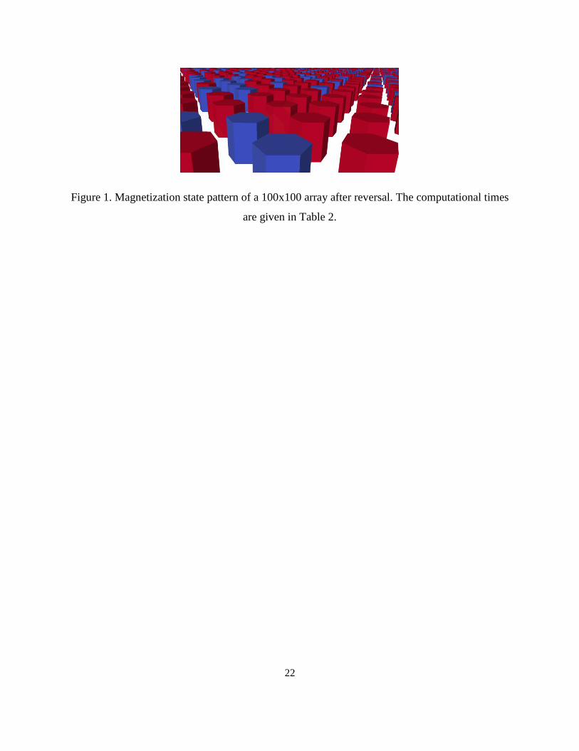
Due to the introduced distributions and magnetostatic interactions not all islands reverse under

the applied field. The resulting pattern for an 100 100 array is shown in Figure 1. The total

number of islands, discretization nodes, tetrahedral elements, and the computational time per

iteration are given in Table 2. It is evident that the computational time scales linearly with the

number of elements starting from a small size. The absolute computational time is small and the

15

largest problem that can be handled is large, especially taking into account that the simulations

were run on inexpensive desktops.

We note that System 2 allowed fitting larger problems, but it also had only around a third of the

computational performance of System 1. The reduced performance was due to the use of CPUs

for sparse products and the older generation GPU. For example, using a computer with a higher-

end Tesla C2070 GPU (with the performance of GeForce GTX 480 but a larger memory of 6

GB) and porting the sparse matrices to run on GPUs on-fly would result in a 3 fold reduction of

the computational time for Mesh 2 and would allow running significantly larger meshes

(estimated at 600 million tetrahedrons) on an inexpensive desktop computer with a single GPU.

This work is ongoing.

We have also considered a complex perpendicular recording head model with a soft underlayer

similar to that reported in Ref. [28], but with a more realistic size (of 5 μm 5 μm 3 μm ).

See the caption to Fig. 2 for details about the head model. This structure was chosen as it

demonstrates several aspects of the FastMag performance, such as its speed and the ability to

handle large problem sizes, non-uniform domains, and complex geometries. It is noted that it

would be hard (or even impossible) to use any currently existing micromagnetic methods and

solvers to model such a complex structure. In particular, FEM based approaches could have

significant convergence and boundary integral complications. FDM approaches could have

significant difficulties in resolving the complex and non-uniform geometries.

We have considered various meshes and show results for two specific meshes. The first mesh

(Mesh 1) had the edge length of around 30 nm and about 4.7 million tetrahedrons. The second

mesh was obtained as a refinement of Mesh 1 to make the edge length of around 10 nm in the

entire head and SUL and it had over 126 million tetrahedrons. We note that we experienced

difficulties in generating very large meshes (over 25 million tetrahedrons) with the mesher used.

These difficulties were overcome by generating smaller meshes determined by the geometry and

writing a refinement code for producing finer meshes determined by the exchange length. This

approach has an added benefit in that it does not require the entire dense mesh information, thus

allowing significantly reducing the peak memory consumption. The simulations for Mesh 1 were

16

run on the fastest System 1 as they were sufficiently small to fit the memory. The simulations for

Mesh 2 were run on System 2 having larger memory (but with around three times slower

performance).

The computational time of these simulations also scales well with the problem size. The absolute

simulation speeds are high. The computational time per simulation time step was 0.42 secs for

Mesh 1 (on System 1) and 36 secs for Mesh 2 (on System 2). Simulating a single switching

occurring on a scale of 200 ps took approximately 151 secs for Mesh 1 and 30 hours for Mesh 2.

Figure 2 shows snapshots of the magnetization state as a colormap for Mesh 1 and Mesh 2 at 97

ps after the switching current was applied. It is evident that the dynamics is different. This

difference was found for all meshes not properly resolving the exchange length, indicating that

proper discretization is important for simulating dynamics in such systems.

7 Summary

We presented FastMag, a fast micromagentic simulator for solving the LLG equation. FastMag

discretizes a general computational domain into tetrahedral elements. The differential operators

are calculated similar to conventional FEM method. The magnetostatic field is computed by

superposition for volume and surface computational domain parts. Efficient quadrature rules and

analytical integration for overlapping elements with singular integral kernel are used to discretize

the superposition integral. The discretized integrals are computed using NGIM with the

computational complexity of ( )VO N . The solver is implemented on Graphics Processing Units,

which offer massive parallelization at a low cost, converting a simple desktop to a powerful

machine matching performance of a CPU cluster. The main features of FastMag are summarized

next.

1) The solver has a high computational speed with computational time scaling linearly from

small to very larger problems.

2) It allows handling very large computational sizes. The largest computational problem size

that can be run on the used systems with 32 GB of CPU RAM and 4GB of GPU memory

is about 150 million tetrahedrons. Increasing the system memory to 128 GB would allow

17

handling up to 0.6 billion tetrahedrons, which is sufficient to accurately model very

complex structures (e.g. realistic recording heads or large arrays).

3) High speed is obtained for general geometries and meshes, e.g. for structured and

unstructured meshes, for uniform and non-uniform meshes, for meshes with small or

large ratios between the surface and volume unknowns, and for geometries with large

empty spaces between magnetic domains distributed regularly or randomly. This makes

FastMag suitable for simulating a host of complex magnetic structures, such as media for

magnetic recording with hard drives and tapes, recording heads, read heads, spin wave

phenomena, arrays of magnetic particles, and magnetic wires, among others.

While the performance of FastMag already allows solving very complex problems, there is a

number of ways the simulator can be enhanced. Implementing the construction of the sparse

matrix-vector products on-fly on GPUs would significantly reduce the memory consumption,

which is critical to fit large problem sizes and increase the speed. In particular, it would

increase by around 3 times the speed of the head simulations with largest Mesh 2 shown in

this paper. It also would increase by around 4 times the largest problem size that can be

handled for a given memory. Using multi-GPU parallelization on shared memory computers,

FastMag can be relatively easily accelerated additionally up to 4 times by simply performing

independent operations on different GPUs in parallel (e.g. sparse products or near- and far-

field components in the dense products). Using multi-GPU distributed memory clusters is

also possible, with a potential to leads to orders of magnitude of further speed-ups and

problem size increases. For example, our estimate is that a relatively inexpensive system with

4 nodes, each comprising 4 GPUs with 3-6 GB GPU memory, 1 quad or hex core CPU, and

128 GB CPU memory, would allow simulating problems of around 2 billion tetrahedrons.

Acknowledgements

The first and second authors contributed equally to the work. Discussions with Thomas Schrefl

and Dieter Suess stimulated the code development.

18

References

[1] K. Z. Gao and H. N. Bertram, "Write field analysis and write pole design in perpendicular

recording," Ieee Transactions on Magnetics, vol. 38, pp. 3521-3527, Sep 2002.

[2] B. Van de Wiele, A. Manzin, O. Bottauscio, M. Chiampi, L. Dupre, and F. Olyslager,

"Finite-Difference and Edge Finite-Element Approaches for Dynamic Micromagnetic

Modeling," Ieee Transactions on Magnetics, vol. 44, pp. 3137-3140, Nov 2008.

[3] R. D. McMichael, M. J. Donahue, D. G. Porter, and J. Eicke, "Comparison of

magnetostatic field calculation methods on two-dimensional square grids as applied to a

micromagnetic standard problem," Journal of Applied Physics, vol. 85, pp. 5816-5818, Apr

1999.

[4] D. R. Fredkin and T. R. Koehler, "Hybrid method for computing demagnetizing fields,"

Ieee Transactions on Magnetics, vol. 26, pp. 415-417, Mar 1990.

[5] J. Fidler and T. Schrefl, "Micromagnetic modelling - the current state of the art," Journal of

Physics D-Applied Physics, vol. 33, pp. R135-R156, Aug 2000.

[6] R. Hertel and H. Kronmuller, "Adaptive finite element mesh refinement techniques in

three-dimensional micromagnetic modeling," Ieee Transactions on Magnetics, vol. 34, pp.

3922-3930, Nov 1998.

[7] W. Scholz, J. Fidler, T. Schrefl, D. Suess, R. Dittrich, H. Forster, and V. Tsiantos,

"Scalable parallel micromagnetic solvers for magnetic nanostructures," Computational

Materials Science, vol. 28, pp. 366-383, Oct 2003.

[8] M. J. Donahue, "Parallelizing a Micromagnetic Program for Use on Multiprocessor Shared

Memory Computers," Ieee Transactions on Magnetics, vol. 45, pp. 3923-3925, Oct 2009.

[9] Y. Kanai, M. Saiki, K. Hirasawa, T. Tsukamomo, and K. Yoshida, "Landau-Lifshitz-

Gilbert micromagnetic analysis of single-pole-type write head for perpendicular magnetic

recording using full-FFT program on PC cluster system," Ieee Transactions on Magnetics,

vol. 44, pp. 1602-1605, Jun 2008.

[10] S. Li, B. Livshitz, and V. Lomakin, "Graphics Processing Unit Accelerated O(N)

Micromagnetic Solver," Ieee Transactions on Magnetics, vol. 46, pp. 2373-2375, June

2010.

[11] T. Sato and Y. Nakatani, "Effect of the calculation precision in micromagnetic simulation,"

in Joint MMM-Intermag Conference, 2010, pp. CF-02.

[12] A. Kakay, E. Westphal, and R. Hertel, "Speedup of FEM Micromagnetic Simulations With

Graphical Processing Units," Ieee Transactions on Magnetics, vol. 46, pp. 2303-2306, Jun

2010.

[13] A. Boag and B. Livshitz, "Adaptive nonuniform-grid (NG) algorithm for fast capacitance

extraction," IEEE Transactions on Microwave Theory and Techniques, vol. 54, pp. 3565-

3570, September 2006.

[14] S. Li, B. Livshitz, and V. Lomakin, "Fast evaluation of Helmholtz potential on graphics

processing units (GPUs)," Journal of Computational Physics, vol. 229, pp. 8463-8483,

2010.

[15] B. Livshitz, A. Boag, H. N. Bertram, and V. Lomakin, "Nonuniform grid algorithm for fast

calculation of magnetostatic interactions in micromagnetics," Journal of Applied Physics,

vol. 105, pp. 07D541 (3 pp.)-07D541 (3 pp.), 1 April 2009.

19

[16] A. F. Peterson, S. L. Ray, and R. Mittra, Computational Methods for Electromagnetics:

IEEE Press, 1997.

[17] D. Suess, V. Tsiantos, T. Schrefl, J. Fidler, W. Scholz, H. Forster, R. Dittrich, and J. J.

Miles, "Time resolved micromagnetics using a preconditioned time integration method,"

Journal of Magnetism and Magnetic Materials, vol. 248, pp. 298-311, July 2002.

[18] M. Gellert and R. Harbord, "Moderate Degree Cubature Formulas for 3D tetrahedral finite-

element approximations," Communications in Applied Numerical Methods, vol. 7, pp. 487-

495, 1991.

[19] S. Balasubramanian, S. N. Lalgudi, and B. Shanker, "Fast-integral-equation scheme for

computing magnetostatic fields in nonlinear media," Ieee Transactions on Magnetics, vol.

38, pp. 3426-3432, Sep 2002.

[20] O. Bottauscio, M. Chiampi, and A. Manzin, "An edge element approach for dynamic

micromagnetic modeling," Journal of Applied Physics, vol. 103, Apr 2008.

[21] S. Li, D. V. Orden, and V. Lomakin, "Fast Periodic Interpolation Method for Periodic Unit

Cell Problems," IEEE Transactions on Antennas and Propagation, vol. 58, pp. 4005-4014,

2010.

[22] NVIDIA, "CUDA Compute Unified Device Architecture Programming Guide, V2.3,"

2009.

[23] ODEPACK. Available: https://computation.llnl.gov/casc/software.html

[24] W. Zhang and S. Haas, "Adaptation and performance of the Cartesian coordinates fast

multipole method for nanomagnetic simulations," Journal of Magnetism and Magnetic

Materials, vol. 321, pp. 3687–3692, 2009.

[25] Y. Takahashi, S. Wakao, T. Iwashita, and M. Kanazawa, "Micromagnetic simulation by

using the fast multipole method specialized for uniform brick elements," Journal of

Applied Physics, vol. 105, Apr 2009.

[26] W. Fong and E. Darve, "The black-box fast multipole method," Journal of Computational

Physics, vol. 228, pp. 8712-8725, Dec 2009.

[27] N. A. Gumerov and R. Duraiswami, "Fast multipole methods on graphics processors,"

Journal of Computational Physics, vol. 227, pp. 8290-8313, Sep 2008.

[28] T. Schrefl, M. E. Schabes, D. Suess, O. Ertl, M. Kirschner, F. Dorfbauer, G. Hrkac, and J.

Fidler, "Partitioning of the perpendicular write field into head and SUL contributions," Ieee

Transactions on Magnetics, vol. 41, pp. 3064-3066, Oct 2005.

20

# of points

(VN )

GPU CPU

Time (S1) Time (S2) Memory Time Memory

4K 0.0012 sec 0.0018 sec 0.14 MB 0.1527 sec 22 MB

260K 0.068 sec 0.118 sec 11.2 MB 7.79 sec 250 MB

1M 0.28 sec 0.56 sec 72MB 30.8 sec 1 GB

67M N/A 53.51 sec 1.8GB N/A N/A

150M N/A 220 sec 3.8GB N/A N/A

Table 1. Computational time and memory consumption of NGIM implemented on CPUs and

GPUs. The times are given for a single evaluation of the potential at VN nodes due to VN

collocated charges distributed in a cube. Times for S1 and S2 refer to simulations run on System

1 and System 2, respectively, as explains in Sec. 6. A linear scaling of the computational time is

obtained from small problems (e.g. 2000 nodes) to very large problems (up to about 70 million

nodes for the available GPUs). The largest achievable size is about 150 million (but it is obtained

under suboptimal NGIM level 6, due to the memory limitations of the used GPU).

21

Array size # of nodes # of tet. Time (S1) Time (S2)

20x20 8.4K 14.4K 1.1e-2 5e-3 sec

50x50 52.5K 90K 2.69e-2 sec 3.5e-2 sec

100x100 210K 360K 6.06e-2 sec 0.143 sec

200x200 840K 1.44M 0.284 sec 0.573 sec

300x300 1.89M 3.24M 0.560 sec 1.29 sec

400x400 3.36M 5.76M N/A 2.33 sec

800x800 13.44M 23.04M N/A 9.35 sec

1600x1600 53.76M 92.16M N/A 40.8 sec

Table 2. Computational time per simulation time step for the case of a square (M M ) array of

magnetic islands. Each island was a hexagonal cylinder with height and largest lateral size of

10 nml . To model material and patterning fluctuations, distributions in island anisotropy and

position were introduced. The mean island anisotropy field and the array’s pitch were

25 kOeKH and 27 nmb , respectively. The random variations for the two quantities were

15% and 10% , respectively. All islands were initially oriented up. An external field of strength

0.91 ext KH H was applied downwards at ο1 to the z -axis over the entire BPM array, where

extH was the switching field of a single island having the mean anisotropy field. The NGIM was

used under the setting of Table 1. The time step was around 1ps. The computational times scale

linear from small to very large arrays. The absolute computational times are small.

22

Figure 1. Magnetization state pattern of a 100x100 array after reversal. The computational times

are given in Table 2.

23

Figure 2. Snapshots of switching process at 97 ps after applying a field for Mesh 1 and Mesh 2.

The color presents the vertical component of the magnetization. The overall dimensions of the

head were 5 μm 5 μm 3 μm (height, width, depth) and the tip lateral size was

65 nm 97 nm with a soft underlayer. The switching was induced by a four-turn coil around

the main pole with a pulsed current. The magnetic material was soft with 31900emu cmsM ,

0.05 , and exchange constant 6 31.5 10 emu cmA . Both the head and underlayer were

meshed and modeled micromagnetically. Mesh 1 had the edge length of around 30 nm and about

4.7 million tetrahedrons. Mesh 2 had the edge length of around 10 nm and over 126 million

tetrahedrons. The NGIM was set to have 256 NG samples with linear interpolation and 64 CG

samples with cubic interpolation, and the number of NGIM levels was 6 and 7 for Mesh 1 and 2,

respectively. For Mesh 1 the computational time per time step was 0.42 sec and the time step

was about 0.55 ps. For Mesh 2, the computational time was 36 sec per time step and the time

step was about 0.07 ps. The magnetization time evolution for the two meshes is different, due to

the fact that Mesh 1 does not represent the magnetization dynamics properly.