Embed Size (px)
Citation preview

EÆcient Kernel Density Estimation Using the
Fast Gauss Transform with Applications to
Segmentation and Tracking
Ahmed Elgammal, Ramani Duraiswami, Larry S. Davis
Computer Vision Laboratory
The University of Maryland
College Park, MD 20742, USA
Abstract
The study of many vision problems is reduced to the estimation of a proba-
bility density function from observations. Kernel density estimation techniques
are quite general and powerful methods for this problem, but have a signi�cant
disadvantage in that they are computationally intensive. In this paper we ex-
plore the use of kernel density estimation with the fast gauss transform (FGT)
for problems in vision. The FGT allows the summation of a mixture ofM Gaus-
sians at N evaluation points in O(M + N) time as opposed to O(MN) time
for a naive evaluation, and can be used to considerably speed up kernel density
estimation. We present applications of the technique to problems from image
segmentation and tracking, and show that the algorithm allows application of
advanced statistical techniques to solve practical vision problems in real time
with today's computers.
1 Introduction
Many problems in computer vision can be posed as obtaining the probability
density function describing an observed random quantity. In general the forms
of the underlying density functions are not known. While classical parametric
densities are mostly unimodal, practical computer vision problems involve mul-
timodal densities. Further, high-dimensional densities can not often be simply
represented as the product of one-dimensional density functions. While mix-
ture methods partially alleviate this problem, they require knowledge about
the problem to choose the number of mixture functions, and their individual
parameters.
An attractive feature of nonparametric procedures is that they can be used
with arbitrary distributions and without the assumption that the forms of the
1

2nd Int'l workshop on Statistical and Computational Theories of Vision 2
underlying densities are known. However, most nonparametric methods require
that all of the samples be stored or that the designer have extensive knowledge
of the problem. Since a large number of samples is needed to obtain good
estimates, the memory requirements can be severe [1].
A particular nonparametric technique that estimates the underlying density
and is quite general is the kernel density estimation technique. In this technique
the underlying probability density function is estimated as
f(x) =Xi
�iK(x� xi) (1)
where K is a \kernel function" (typically a Gaussian) centered at the data
points, xi; i = 1::n and �i are weighting coeÆcients (typically uniform weights
are used, i.e., �i = 1=n). Note that choosing the Gaussian as a kernel function is
di�erent from �tting the distribution to a Gaussian model. Here, the Gaussian
is only used as a function that is weighted around the data points. The use of
such an approach requires a way to eÆciently evaluate the estimate f(xj) at
any new point xj . A good discussion of kernel estimation techniques can be
found in [2].
In general, given N original data samples and M points at which the den-
sity must be evaluated, the complexity is O(NM) evaluations of the kernel
function, multiplications and additions. For many applications in computer vi-
sion, where both real-time operation and generality of the classi�er are desired,
this complexity can be a signi�cant barrier to the use of these density estimation
techniques. In this paper we discuss the application of an algorithm, the Fast
Gauss Transform (FGT) [3, 4], that improves the complexity of this evaluation
to O(N +M) operations, to computer vision problems.
The FGT is one of a class of very interesting and important new families
of fast evaluation algorithms that have been developed over the past dozen
years, and are revolutionizing numerical analysis. These algorithms use the fact
that all computations are required only to a certain accuracy (which can be
arbitrary) to speed up calculations. These algorithms enable rapid calculation
of approximations of arbitrary accuracy to matrix-vector products of the form
Ad where aij = �(jxi � xj j) and � is a particular special function. These
sums �rst arose in applications that involve potential �elds where the functions
� were spherical harmonics, and go by the collective name \fast multipole"
methods [3]. The basic idea is to cluster the sources and target points using
appropriate data structures, and to replace the sums with smaller summations
that are equivalent to a given level of precision. Interesting applications of these
algorithms include fast versions of Fourier transforms that do not require evenly
spaced data points [5]. An algorithm for evaluating Gaussian sums using this
technique was developed by Greengard and Strain [4]. We will be concerned
with this algorithm and its extensions in this paper. Related work also includes
the work by Lambert et al [6] for eÆcient on-line computation of kernel density
estimation.
Section 2 introduces some details of the Fast Gauss Transform, and our im-
provements to it. We also present practical demonstrations of the improvement

2nd Int'l workshop on Statistical and Computational Theories of Vision 3
in complexity. In Section 3 we introduce using kernel density estimation to
model the color of homogenous regions and use this approach to segment fore-
ground region corresponding to people into major body parts. In Section 4 we
show how the fast Gauss algorithm can be used to eÆciently compute estimates
for density gradient and use this for tracking people. The tracking algorithm is
robust to partial occlusion and rotation in depth and can be used with station-
ary or moving cameras. Appropriate reviews of the relevant related work are
provided in these self-contained sections.
2 Fast Gauss Transform
The FGT was introduced by Greengard and Strain [3, 4] for the rapid evaluation
of sums of the form
S (ti) =
NXj=1
fj exp
�(sj � ti)
2
�2
!; i = 1; : : : ;M: (2)
Here sj and ti are respectively the d�dimensional \source" and \target" coor-
dinates, while � is a scalar and fj are source strengths. They showed that using
their fast algorithm this sum could be computed in O(N+M) operations. They
also showed results from 1-D and 2-D tests of the algorithm. It was extended by
Strain [7] to sums where � in equation 2 varied with the position of the target
or the source, i.e., for the case where � depends on the source location the sum
is
S (ti) =
NXj=1
fj exp
�(sj � ti)
2
�2j
!; i = 1; : : : ;M: (3)
A puzzling aspect of the FGT is that even though the algorithm was pub-
lished fourteen years ago, and Gaussian mixture sums arise often in statistics
(as already noted by Greengard and Strain), the algorithm has not been used
much in applications. Subsequent publications on the FGT have only begun to
appear again over the last two years.
An important reason for the lack of use of the algorithm is probably the
fact that it is inconvenient to do so. First, it is not immediately clear what the
cross-over point is when the algorithm begins to manifest its superior asymptotic
complexity and o�sets the pre-processing overhead. While the nominal complex-
ity of the algorithm is O(M + N);the constant multiplying it is O(pd), where
p is the number of retained terms in a polynomial approximation (described
below). This makes it unclear if the algorithm is useful for higher dimension
applications seen in statistical pattern recognition. The fact that there is no
readily available implementation to test these issues acts as a further barrier to
its wide adoption.
Another reason for the delay in applying the FGT to problems in compu-
tational statistics might be that the algorithm, as originally presented, are not
directly applicable to general mixture of gaussian sums that statisticians are

2nd Int'l workshop on Statistical and Computational Theories of Vision 4
used to thinking about. General d�dimensional mixture of gaussian sums have
the form
S(ti) =
NXj=1
fj exp�� (ti � sj)
0
V �1 (ti � sj)�
(4)
with V �1 is a symmetric positive de�nite covariance matrix, which is much more
complex than 2. Even in the case of kernel density estimation with Gaussians,
the form of the Gaussian sum encountered is
S(ti) =
NXj=1
fje�
Pdk=1
�(ti�sj)k
�k
�2
=
NXj=1
fje�
��(ti�sj)1
�1
�2
+:::+
�(ti�sj)d
�d
�2�; (5)
where the subscript k indicates the component along the kth coordinate axis,
i.e., the covariance matrix is diagonal. The applications we present below in
segmentation and tracking use this form which is a generalization over the orig-
inal FGT algorithm. Our ongoing work (the details of which, including a proof
of convergence are to be reported elsewhere) extends the variable scale FGT
algorithm to sums of the form 5.
2.1 Speeding up computations with Gaussians
Before describing the FGT, it is appropriate to describe some algorithmic im-
provements for evaluating Gaussian mixture sums proposed in the literature,
which are distinct from the FGT.
The evaluation of a special function such as the exponential is usually ex-
pensive, requiring ~O(100) oating point operations using the normal libraries
supplied with compilers. Approximate libraries that achieve accuracy almost
everywhere, and require fewer oating point operations are available, e.g., the
Intel approximate math library [8] claims a speedup of a factor of 5 for eval-
uating exponentials over the corresponding x87 implementation. The FGT is
distinct from these, and indeed the approximate math libraries can be used in
conjunction with it to achieve further speed-up.
A second speed-up of gaussian sums is based on the observation that since
a Gaussian typically decays relatively quickly, leading to insigni�cant additions
when it is evaluated beyond a speci�ed distance, heuristics can be used to avoid
unnecessary evaluations when ��1 (js� tj) is small. Some authors (e.g., Fritsch& Rogina, 1996 [9]) have formalized this by developing a data structure that
enables automating this heuristic. The FGT also employs such data structures,
and automates the observation that lies behind this heuristic by providing rig-
orous error bounds.

2nd Int'l workshop on Statistical and Computational Theories of Vision 5
2.2 Overview of the Algorithm
The shifting identity that is central to the algorithm is a re-expansion of the
exponential in terms of a Hermite series by using the identity
e�(t�s� )
2
= e�
�t�s0�(s�s0)
�
�2= e�(
t�s0� )
21Xn=0
1
n!
�s� s0
�
�nHn
�t� s0
�
�; (6)
where Hn are the Hermite polynomials. This formula tells us how to evaluate
the Gaussian �eld exp���t�s�
�2�at the target t due to the source at s, as an
Hermite expansion centered at any given point s0: Thus a Gaussian centered at
s can be shifted to a sum of Hermite polynomials times a Gaussian, all centered
at s0: The series converges rapidly and for a given precision only p terms need
to be retained. The quantities t and s can be interchanged to obtain a Taylor
series around the target location as
e�(t�s� )
2
= e�
�t�t0�(s�t0)
�
�2'
pXn=0
1
n!hn
�s� t0
�
��t� t0
�
�n: (7)
where the Hermite functions hn (t)are de�ned by
hn (t) = e�t2
Hn (t) : (8)
The algorithm achieves its gain in complexity by avoiding evaluating every
Gaussian at every evaluation point (which leads to O(NM) operations). Rather,
equivalent p term series are constructed about a small number of source cluster-
centers using Equation 6 (for O(Npd) operations). These series are then shifted
to target cluster-centers, and evaluated at theM targets in O(Mpd) operations.
Here the number of terms in the series evaluations, p; is related to the desired
level of precision �, and is typically small as these series converge quickly.
The process is illustrated in Figure 1. The sources and targets are divided
into clusters using a simple boxing operation. This permits the division of the
Gaussians according to their locations The domain is scaled to be of O(1), and
the box sizes are chosen to be of size rp2� where r is a scale parameter.
Since Gaussians decay rapidly, sources in a given box will have no e�ect (in
terms of the desired accuracy) to targets relatively far from there sources (in
terms of distance scaled by the standard deviation �). Therefore the e�ect of
sources in a given box need to be computed only for targets in close boxes. Given
the sources in one box and the targets in a neighboring box, the computation
is performed using one of the following four methods depending on the number
of sources and targets in these boxes: Direct evaluation is used if the number
of sources and targets are small. If the sources are clustered in a box then
they can be transformed into Hermite expansion about the center of the box
using equation 6. This expansion is directly evaluated at each target if the
number of the targets is small. If the targets are clustered then the sources or
their expansion are converted to a local Taylor series (equation 7) which is then

2nd Int'l workshop on Statistical and Computational Theories of Vision 6
Figure 1: The fast gauss transform performs gaussian sums to a prescribed
degree of accuracy by using either direct evaluations of the Gaussian for isolated
sources and targets, or consolidates sources with Hermite series evaluation at
isolated targets, or consolidates many sources near a clustered target location
via Taylor series, or combines Hermite and Taylor series for clustered sources
and targets.
evaluated at each target in the box. The number of terms to be retained in
the series, p, depends on the required precision, the box size scale parameter
r and the standard deviation �. The break-even point when using expansion
is more eÆcient than direct evaluation is O(pd�1). Further details may be
obtained from [4]. The clustering operation is aided by the use of appropriate
data structures.
2.3 Fast Gauss Transform Experimental Results
Before presenting applications of the FGT to vision problems, we present some
experimental results, that illustrate further how the algorithm achieves its speedup.
The �rst experiment compares the performance of the FGT with di�erent choices
of the required precision � with direct evaluation for a 2D problem. Table 1 and
Figure 2 shows the CPU time using direct evaluation versus that using FGT
for di�erent precisions, � = 10�4; 10�6; and 10�8 for sources with � = 0:05.

2nd Int'l workshop on Statistical and Computational Theories of Vision 7
The box size scale parameter r was set to 0.51. The sources and targets were
uniformly distributed in the range [0,1] and the strength of the sources were
random between 0 and 1. Table 2 shows the division of work between the di�er-
ent components of the FGT algorithm for the � = 10�6 case. From the division
of work we notice that for relatively small number of sources and targets only
direct evaluation is performed. Although, in this case, the algorithm performs
only direct evaluations, it gives �ve to ten times speed up when compared with
direct evaluation because of the way the algorithm divides the space into boxes
and the locality of the direct evaluation based on the desired precision. i.e.,
the FGT algorithm does a smart direct evaluation. This is comparable to the
speed-ups reported by Fritsch and Rogina with their bucket-box data structure.
As the number of sources and targets increases and they become more clus-
tered, other evaluation decisions are made by the algorithm, and the algorithm
starts to show the linear (O(N +M)) performance. For very large number of
sources and targets, the computation are performed through Hermite expan-
sions of sources transformed into Taylor expansions as described above, and
this yields a signi�cant speedup. For example, for N =M = 105, the algorithm
gives more than 800 time speedup than direct evaluation for 10�4 precision.
From the �gures we also note that the FGT starts to outperform direct
evaluation for number of sources and targets as low as 60-80 based on the desired
accuracy. This break-even point can be pushed further down by increasing the
box size scale parameter, r. This will enhance the performance of the algorithm
for small N;M but will worsen the asymptotic performance.
Direct Fast Gauss
N=M Evaluation � = 10�4 � = 10�6 � = 10�8
50 0.7 0.8 0.9 1.1100 2.7 1.3 1.7 2.0200 10.8 2.9 3.7 4.6400 43 8.2 10.8 14800 174 27 36 461600 689 96 130 1633200 2754 319 493 6406400 11917 660 1281 193512800 58500 942 2022 3277
25600 234x 103 1429 3210 5113
51200 936x 103 2405 5602 8781
102400 3744x 103 4382 10410 16181
204800 14976x 103 8428 20191 31106
1024000 374x 106 43843 100263 153791
Table 1: Run time in milliseconds for direct evaluation vs. FGT with di�erentprecision
Figure 3 shows the performance of the algorithm for cases where the sources
and the targets are clustered di�erently. The direct evaluation is compared with
1The software was written in Visual C++ and the results were obtained on a 700MHz Intel
Pentium III PC with 512 MB RAM.

2nd Int'l workshop on Statistical and Computational Theories of Vision 8
102
103
104
105
106
10−4
10−2
100
102
104
106
N=M
seco
nds
Direct evaluationFGT tol = 1e−8 FGT tol = 1e−6 FGT tol = 1e−4
Figure 2: Run time for direct evaluation vs. FGT with di�erent precision
Division of work (%) - Uniform sources and targets
Direct Taylor Hermit Hermit + TaylorN=M Evaluation Expansion Expansion Expansion
� 800 100 0 0 01600 96.6 1.6 1.8 03200 65.7 15.6 15 3.76400 5.3 18.3 16.9 59.512800 0 0.3 0.3 99.4� 25600 0 0 0 100
Table 2: Division of work between di�erent computational methods for uni-formly distributed random sources and targets
the FGT for three con�gurations of sources and targets: in the �rst case, the
sources and targets are uniformly distributed between 0 and 1. In the second
case the sources are clustered inside a circle of radius 0.1 and the targets are
uniformly distributed between 0 and 1. In the third case, both the sources
and the targets are clustered inside a circle of radius 0:1. For all three cases the
desired precision was set to 10�6, the sources have a scale � = 0:05 and a random
strength between 0 and 1. The division of work for the three cases are shown
in Tables 2, 3, and 4. From the �gures we note that for the cases where sources
and/or targets are clustered the computation shows linear time behavior for
number of sources and targets as low as 100, which yields a signi�cant speedup.
For a very large number of sources and targets, the computations are performed
through Hermite expansions of sources transformed into Taylor expansions.
Figure 4 shows the same experiment with the three con�gurations of sources
and targets for the 3D case with precision set to 10�6 and r = 0:5. Note that the

2nd Int'l workshop on Statistical and Computational Theories of Vision 9
102
103
104
105
106
10−4
10−2
100
102
104
106
N=M
seco
nds
Direct evaluation FGT: uniform sources & targets FGT: Clustered sources FGT: Clustered sources & targets
Figure 3: Run time for FGT with di�erent con�guration of sources and targets
layout
Division of work (%) - Clustered sources, Uniform targets
Direct Taylor Hermit Hermit + TaylorN=M Evaluation Expansion Expansion Expansion
100 83.7 0 16.3 0200 65.2 0 34.8 0400 32.7 0 67.3 0800 21.3 0 78.7 01600 17.1 0.3 81.4 1.23200 9.2 2.7 69.2 18.96400 1.8 5.6 22.5 70.112800 0 2.6 0.4 97� 25600 0 0 0 100
Table 3: Division of work between di�erent computational methods for clusteredsources and uniformly distributed targets
algorithm starts to utilize computations using Hermite and/or Taylor expansion
only when the number of sources and/or targets in a box exceeds a break point
of order pd�1 which is higher in the 3D case. This causes the algorithm to do
mostly direct evaluation for the uniform sources and targets case while Hermite
and Taylor expansion computations were utilized for large number of clustered
sources and/or targets.
Figure 5 shows e�ect of the source scale on the run time of the FGT algo-
rithm. The �gure shows the run time for three cases where sources have scale
� = 0:1; 0:05; 0:01. For all the cases, the sources and targets were uniformly
distributed between 0 and 1. The box size scale parameter was set to r = 0:5
for all the cases. The run time in all the cases converges asymptotically to the
linear behavior.

2nd Int'l workshop on Statistical and Computational Theories of Vision 10
Division of work (%) - Clustered sources and targets
Direct Taylor Hermit Hermit + TaylorN=M Evaluation Expansion Expansion Expansion
100 69.4 13.9 13.9 2.8200 36.9 28.7 19.3 15.1400 12.7 21.6 24.4 41.3800 4.8 16.8 17.4 61.01600 2.8 15.1 13.0 69.13200 2.2 10.3 15.3 72.26400 0.8 6.8 9.3 83.112800 0.1 2.4 2.4 95.1� 25600 0 0 2.4 97.6
Table 4: Division of work between di�erent computational methods for clusteredsources and targets
102
103
104
105
10−3
10−2
10−1
100
101
102
103
104
105
N=M
seco
nds
Direct evaluation FGT: uniform sources & targets FGT: clustered sources, uniform FGT:clustered sources & targets
Figure 4: Run time for 3D - FGT with di�erent con�guration of sources and
targets layout
3 Region Segmentation via Color Modeling
3.1 Color Density Estimation
In this application we utilize the fast Gauss algorithm for eÆcient density es-
timation of color distribution of a region. We use this approach to model the
color distribution on people's clothing and to segment major body parts based
on clothing. A variety of parametric and non-parametric statistical techniques
have been used to model the color and the spatial properties of colored regions.
In [10] the color properties of a region (blob) were modeled using a single Gaus-
sian in the three dimensional Y UV space. The use of a single Gaussian to
model the color of a blob restricts the blob to be of a single color which is not a
general enough assumption about the clothes people wear which usually contain

2nd Int'l workshop on Statistical and Computational Theories of Vision 11
102
103
104
105
106
10−4
10−2
100
102
104
106
N=M
seco
nds
Direct EvaluationFGT: scale = 0.1 FGT: scale = 0.05FGT: scale = 0.01
Figure 5: Run time for 2D - FGT with uniformly distributed sources and targets
with di�erent scales.
patterns and have many colors. Fitting a mixture of Gaussian using the EM al-
gorithm provides a way to model blobs with a mixture of colors. This technique
was used in [11, 12] for color based tracking of a single blob and was applied for
tracking faces. The mixture of Gaussian technique faces the problem of choosing
the right number of Gaussians for the assumed model. Non-parametric tech-
niques using histograms have also been used for modeling color distributgions.
In [13] 3-dimensional adaptive histograms in RGB space were used to model
the color of the whole person. Color histograms have also been used in [14]
for tracking hands. The major drawback with color histograms is the lack of
convergence to the right density function if the data set is small.
We use a non-parametric approach to model the color distribution of a uni-
form region. Given a sample S = fxig taken from the region where i = 1:::N
and xi is a d-dimensional vector representing the color, we can estimate the
density function at any point y of the color space directly from S using kernel
density estimation [2]
P (y) =1
N�1:::�d
NXi=1
dYj=1
K
�yj � xij
�j
�; (9)
where the same kernel function is used in each dimension with a di�erent band-
width �j for each dimension of the color space.
Theoretically, kernel density estimators can converge to any density shape
with enough samples [2]. Unlike histograms, even with a small number of sam-
ples, kernel density estimation leads to a smooth continuous density estimate. If
the underlying distribution is a mixture of Gaussians, kernel density estimation
converges to the right density with a small number of samples. Unlike paramet-
ric �tting of a mixture of Gaussians, kernel density estimation is a more general
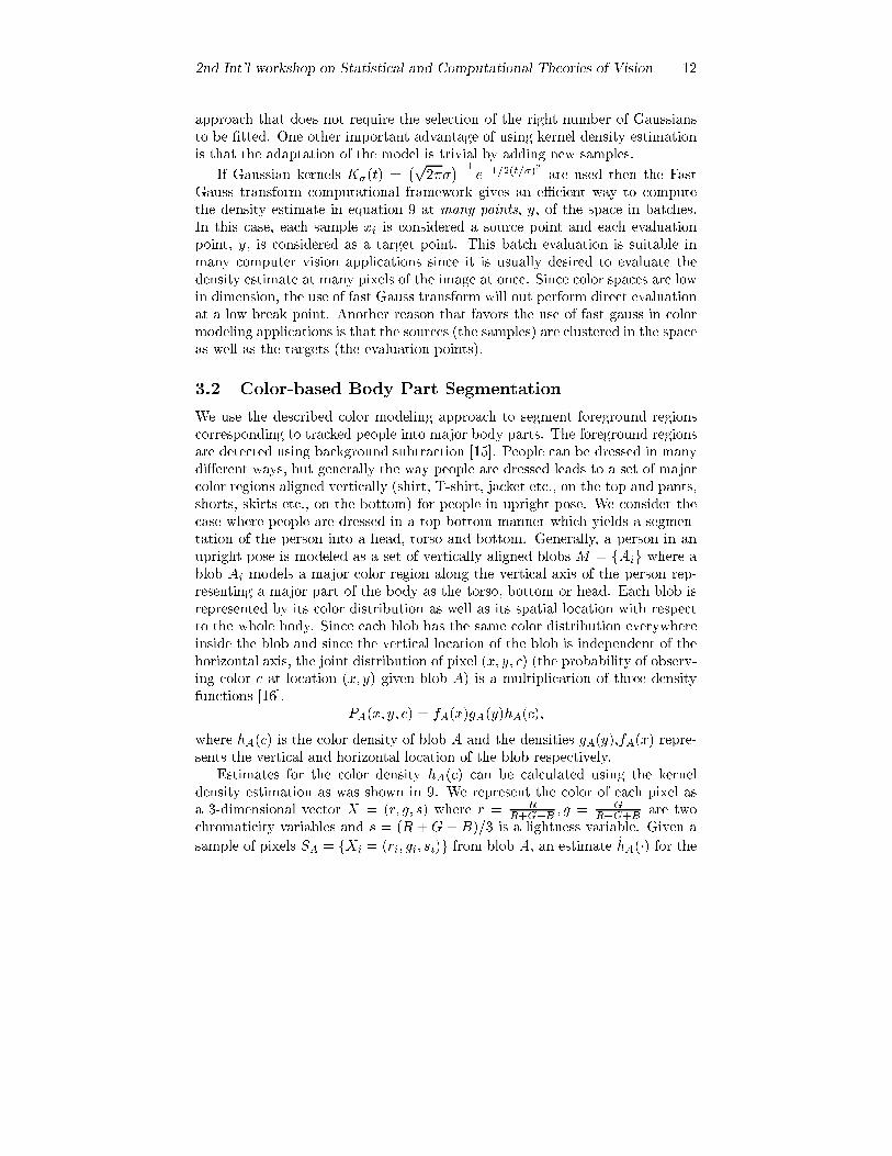
2nd Int'l workshop on Statistical and Computational Theories of Vision 12
approach that does not require the selection of the right number of Gaussians
to be �tted. One other important advantage of using kernel density estimation
is that the adaptation of the model is trivial by adding new samples.
If Gaussian kernels K�(t) =�p
2����1e�1=2(t=�)
2
are used then the Fast
Gauss transform computational framework gives an eÆcient way to compute
the density estimate in equation 9 at many points, y, of the space in batches.
In this case, each sample xi is considered a source point and each evaluation
point, y, is considered as a target point. This batch evaluation is suitable in
many computer vision applications since it is usually desired to evaluate the
density estimate at many pixels of the image at once. Since color spaces are low
in dimension, the use of fast Gauss transform will out perform direct evaluation
at a low break point. Another reason that favors the use of fast gauss in color
modeling applications is that the sources (the samples) are clustered in the space
as well as the targets (the evaluation points).
3.2 Color-based Body Part Segmentation
We use the described color modeling approach to segment foreground regions
corresponding to tracked people into major body parts. The foreground regions
are detected using background subtraction [15]. People can be dressed in many
di�erent ways, but generally the way people are dressed leads to a set of major
color regions aligned vertically (shirt, T-shirt, jacket etc., on the top and pants,
shorts, skirts etc., on the bottom) for people in upright pose. We consider the
case where people are dressed in a top-bottom manner which yields a segmen-
tation of the person into a head, torso and bottom. Generally, a person in an
upright pose is modeled as a set of vertically aligned blobs M = fAig where a
blob Ai models a major color region along the vertical axis of the person rep-
resenting a major part of the body as the torso, bottom or head. Each blob is
represented by its color distribution as well as its spatial location with respect
to the whole body. Since each blob has the same color distribution everywhere
inside the blob and since the vertical location of the blob is independent of the
horizontal axis, the joint distribution of pixel (x; y; c) (the probability of observ-
ing color c at location (x; y) given blob A) is a multiplication of three density
functions [16].
PA(x; y; c) = fA(x)gA(y)hA(c);
where hA(c) is the color density of blob A and the densities gA(y),fA(x) repre-
sents the vertical and horizontal location of the blob respectively.
Estimates for the color density hA(c) can be calculated using the kernel
density estimation as was shown in 9. We represent the color of each pixel as
a 3-dimensional vector X = (r; g; s) where r = RR+G+B
; g = GR+G+B
are two
chromaticity variables and s = (R +G + B)=3 is a lightness variable. Given a
sample of pixels SA = fXi = (ri; gi; si)g from blob A, an estimate hA(�) for the

2nd Int'l workshop on Statistical and Computational Theories of Vision 13
color density hA(�)can be calculated as
hA(r; g; s) =1
N
NXi=1
K�r(r � ri)K�g (g � gi)K�s(s� si);
whereK�(t) = 1=�K(t=�). Using Gaussian kernels, i.e.,K�(t) =�p
2����1e�1=2(t=�)
2
with di�erent bandwidths in each dimension, the density estimation can be eval-
uated as a sum of Gaussians as
hA(r; g; s) =1
N� C
NXi=1
e�1=2(r�ri�r
)2e�1=2(
g�gi�g
)2
e�1=2(s�si�s
)2
where C is a constant. At each new frame, it is desired to evaluate this proba-
bility at di�erent locations. The FGT algorithm is used to eÆciently compute
these probabilities. Here the sources are the sample locations SA;while the tar-
gets are the vectors (r; g; s) at each evaluation location. The estimation of the
bandwidths for each dimension is done o�ine by considering batches of regions
with a single color distribution taken from images of people's clothing and es-
timating the variance in each color dimension. This model is not restricted to
a particular color space, and can be extended to any three dimensional color
space.
Given a set of samples S = fSAig corresponding to each blob and initial
estimates for the position of each blob yAi, each pixel is classi�ed into one of
the three blobs based on maximum likelihood classi�cation assuming that all
blobs have the same prior probabilities
X 2 Ak s.t. k =argkmaxP (X j Ak)
= argkmax gAk(y)hAk
(c) (10)
where the vertical density gAk(y) is assumed to have a Gaussian distribution
gAk(y) = N(yAk
; �Ak). Since the blobs are assumed to be vertically above each
other, the horizontal density fA(x) is irrelevant to the classi�cation.
A horizontal blob separator is detected between each two consecutive blobs
by �nding the horizontal line that minimizes the classi�cation error. Given the
detected blob separators, the color model is recaptured be sampling pixels from
each blob. Blob segmentation is performed and blob separators are detected at
each new frame as long as the target is isolated and tracked.
Model initialization is done automatically by taking three samples S =
fSH ; ST ; SBg of pixels from three con�dence bands corresponding to the head,
torso and bottom. The locations of these con�dence bands are learned o�ine
as follows: A set of training data2 is used to learn the location of blob sepa-
rators (head-torso, torso-bottom) with respect to the body for a set of people
in upright pose where these separators are manually marked. Figure 6-a shows
2The training data consists of 90 samples of di�erent people from both genders in di�erent
orientations in upright pose.

2nd Int'l workshop on Statistical and Computational Theories of Vision 14
0 0.2 0.4 0.6 0.8 10
0.005
0.01
0.015
0.02
0.025
Propotional height
Fre
quen
cy Head Torso Bottom
a b c d
Figure 6: a- Blob separator histogram from training data. b- Con�dence bands.
c - Blob segmentation. d- Detected blob separators
a histogram of the locations of head-torso (left peak) and torso-bottom (right
peak) in the training data. Based on these separator location estimates, we can
determine the con�dence bands proportional to the height where we are con�-
dent that they belong to head, torso and bottom and use them to capture initial
samples S = fSH ; ST ; SBg. Figure 6-b shows initial bands used for initializationwhere the segmentation result is shown in 6-c and the detected separators are
shown in 6-d.
Figure 7: Example results for blob segmentation
Figure 7 illustrates some blob segmentation examples for various people. No-
tice that the segmentation and separator detection is robust even under partial
occlusion of the target as in the rightmost result. Also in some of these examples
the clothes are not of a uniform color. In [16] we showed how this representation
can be used to segment foreground regions corresponding to multiple people in
occlusion.

2nd Int'l workshop on Statistical and Computational Theories of Vision 15
4 People Tracking Application
In this application we show how the fast Gauss transform algorithm can be used
to eÆciently compute estimate for the gradient of the density as well as estimate
for the density itself. Estimation of density gradient is useful in applications
that use the mean shift algorithm [17, 18, 19, 20]. We utilize the color-spatial
joint distribution of a region as a constraint that is used to locate that region
in subsequent frames and therefore to track this region. The color-spatial joint
density is estimated using kernel density estimation. An estimate of the gradient
of the joint density is used to drive a gradient based search that is used to track
that region. In order to reduce the dimensionality of the problem, we use one
spatial dimension and two color dimensions to represent the joint color-spatial
density. This is justi�ed, since for the majority of clothing for people in upright
pose, the color distribution is independent of the horizontal axis and depends
only on the vertical axis. That is, we are most likely to observe the same color
distribution orthogonal to the vertical axis. (Note that this does not assume
constant horizontal color). This allows us to use only the vertical dimension in
our representation of the joint color-spatial density. The independence of the
color distribution from the abscissa makes the representation robust to rotation
in depth.
Let S = fXigi=1::n be a set of sample pixels from the target region so
that Xi = (xi; yi; ui) where xi; yi is the sample pixel location around an origin
o, and ui 2 Rd is a d-dimensional color vector. Given the sample S as a
model for the target region, the joint spatial-color probability of observing a
pixel X at location (x; y) with color u can be expressed as two independent
density functions (since the color distribution is assumed to be independent of
the horizontal axis and depends only on the vertical axis)
P (x; y; u) = F (x)H(y; u); (11)
where H(y; u) represents the joint density between the vertical location and
the color features and F (x) represents the distribution along the horizontal
axis. If we use two chromaticity variables u = (u1; u2) with diagonal covariance
matrix to represent the color for each pixel, then we can estimate joint density
H(y; u j S) as:
H(y; u) =1
N
NXi=1
K�y (y � yi)K�u1(u1 � ui1)K�u2
(u2 � ui2);
where �y; �u1 ; �u2 are the kernel bandwidths in the three dimensions. Given a
translation of the region origin to a location (xc; yc) and a scaling hc, we can
estimate the probability of a pixel X = (x; y; u) coming from S by shifting and
scaling as
H(yc;hc)(y; u) =1
N
NXi=1
K�y
�y � yc
hc� yi
�K�u1
(u1� ui1)K�u2(u2� ui2): (12)

2nd Int'l workshop on Statistical and Computational Theories of Vision 16
Let R(c) be a region that represents the target with respect to a location
and a scaling hypothesis c = (xc; yc; hc), we de�ne the likelihood function (c)
by integrating log probabilities over R as:
(c) =
ZR
wc(x; y)L(Pc(x; y; u))dx (13)
where Pc(x; y; u) is an estimate of the joint density in 11, L(�) is a log functionand wc(x; y) is a weight kernel. Practically, we can assign more weights to pixel
inside the region and less weights for pixels on the region boundary since their
inclusion in R is expected to be noisy. The target localization at frame t can be
formalized as a search for a 2-D translation and a scaling that maximizes (c).
i.e., the location and scale hypothesis c = (xc; yc; hc) that maximizes (c):
c = argcmax (c)
Given the joint density in equation 11 the likelihood function can be written as
(c) =X
(x;y;u)2R
wc(x; y)L(Fc(x)) + wc(x; y)L(Hc(y; u)) (14)
We can drop the �rst term since this will be the same for all hypotheses, and
so we can rede�ne (:) in a simpler way as
(c) =X
(x;y;u)2R
wc(x; y)L(Hc(y; u)) (15)
For the weights wc(x; y), we use Gaussian kernels N(xc; �xhc); N(yc; �yhc)
where �x; �y are scaling constants in the horizontal and vertical direction.
0
50
100
150
200
250
300
350
0
50
100
150
200
2500
2
4
6
8
a) original image b) plot of surface (c)
Figure 8: Likelihood function surface
The optimal target hypothesis represents a local maxima in the discrete three
dimension search space. The log likelihood function is continuous and di�eren-
tiable and, therefore, a gradient based optimization technique would converge
to that solution as long as the initial guess is within a small neighborhood of
that maxima. Figure 8 shows a plot of the function (c) for each location in

2nd Int'l workshop on Statistical and Computational Theories of Vision 17
the image as a hypothesis for the target origin. For this plot, R was de�ned as
a vertical ellipse of the same size as the target.
The derivation of the gradient of the objective function yields (after some
manipulation):
(�xh)2 �
rx (c)
(c)=
P(x;y) xwc(x; y)L(Hc)P(x;y)wc(x; y)L(Hc)
� xc
(�yh)2 �
ry (c)
(c)=
0@(�yh)2
P(x;y)wc(x; y)
ryHc
HcP(x;y)wc(x; y)L(Hc)
+
P(x;y) ywc(x; y)L(Hc)P(x;y)wc(x; y)L(Hc)
!� yc
where the termryHc
Hc
is the normalized gradient of the joint density Hc which
can be derived from equation 12 and can be expressed as
ryHc(x; y; u)
Hc(x; y; u)=
�1�2h
� (16)
PNi=1 xiK�y (
y�ychc
� yi)K�u1(u1 � ui1)K�u2
(u2 � ui2)PNi=1K�y (
y�ychc
� yi)K�u1(u1 � ui1)K�u2
(u2 � ui2)�y � yc
hc
!
The main computation overhead is the calculation of the joint density esti-
mate Hc(y; u1; u2) and its gradient, ryHc(x; y; u). That is, the evaluation of
Gaussian summation
S1(�y; u1; u2) = C1
NXi=1
e�
12(�y�yi�y
)2
e�
12(u1�ui1�u1
)2
e�
12(u2�ui2�u2
)2
and a weighted version of it
S2(�y; u1; u2) = C2
NXi=1
yie�
12(�y�yi�y
)2
e�
12(u1�ui1�u1
)2
e�
12(u2�ui2�u2
)2
Where C1,C2 are normalization constants and N is the number of samples in
the target model. At each iteration We need to evaluate these sums at each
pixel (x; y; u1; u2) in the region de�ned by each new region origin hypothesis
c = (xc; yc; hc) where �y = y�ychc
. These summation is evaluated using Fast
Gauss algorithm where the sources are the sample points (yi; ui1; ui2)i=1::n and
the targets are the evaluation pixels (y; u1; u2) in candidate region R(c). Notice
that in the second summation each source is assigned a strength yi=PN
i=1 yiTo achieve eÆcient implementation, we developed a two phase version of the
fast Gauss algorithm where in the �rst phase all the source data structures and
expansions are calculated from the samples. Then, at each new frame, these

2nd Int'l workshop on Statistical and Computational Theories of Vision 18
Figure 9: Tracking result
structures and expansions are reused to evaluate the new targets. Since targets
(evaluation points) are expected to be similar from frame to frame, the results of
each evaluation are kept in a look up table to avoid doing repeated computation.
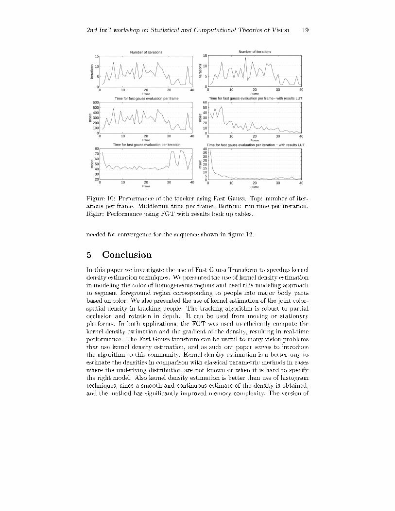
Figure 9 shows four frames from the tracking result for a sequence. The
sequence contains 40 frames taken at about 5 frames per second rate. The
tracker successfully locate the target at this low frame rate. Notice that the
target changes his orientation during the tracking. Figure 10-left shows the
performance of the tracker on this sequence using Fast Gauss only (no look up
tables). The average run-time per frame is about 200-300 msec. Figure 10-right
shows the performance of the tracker with look up tables used in conjunction
with fast Gauss transform to save repeated computation. In this case, the run
time decreases with time and the average run time per frame is less than 20
msec. This is more than 10 times speed up per iteration.
Figure 11 shows examples of tracking under partial occlusion. The target in
this case is waiting for the elevator and is not moving signi�cantly. The results
shows that the tracker continued to locate the target successfully throughout
several signi�cant occlusion situation. Notice also that the horizontal location of
the located region is not a�ected if some parts of the body are occluded. Since
there is no signi�cant motion in most of these sequence, motion based tracking
would fail in such a sequence. Also algorithms based on adaptive background
subtraction might adapt to the target. Figure 12 shows results of tracking a
person in a crowd. These results are for videos captured at 10-12 frame per
second. The tracker successfully locates the targets at this low frame rate. The
bandwidths for the joint distribution kernels were set to 5%, 1%, 1% of each
dimension space size for �y,�u1 and �u1 respectively. The weight kernel w is
narrow in the horizontal direction (�x = 0:5 � width2
) and wide in the vertical
direction (�y = 1:8 � height2
). Figure 13 shows a plot of the number of iterations
2nd Int'l workshop on Statistical and Computational Theories of Vision 19
0 10 20 30 400
5
10
15
Frameite
ratio
ns
Number of iterations
0 10 20 30 400
100200300400500600
Frame
mse
c
Time for fast gauss evaluation per frame
0 10 20 30 4020304050607080
Frame
mse
c
Time for fast gauss evaluation per iteration
0 10 20 30 400
5
10
15
Frame
itera
tions
Number of iterations
0 10 20 30 400
102030405060
Frame
mse
c
Time for fast gauss evaluation per frame− with results LUT
0 10 20 30 4005
10152025303540
Frame
mse
c
Time for fast gauss evaluation per iteration − with results LUT
Figure 10: Performance of the tracker using Fast Gauss. Top: number of iter-
ations per frame. Middle:run time per frame. Bottom: run time per iteration.
Right: Performance using FGT with results look up tables.
needed for convergence for the sequence shown in �gure 12.
5 Conclusion
In this paper we investigate the use of Fast Gauss Transform to speedup kernel
density estimation techniques. We presented the use of kernel density estimation
in modeling the color of homogeneous regions and used this modeling approach
to segment foreground region corresponding to people into major body parts
based on color. We also presented the use of kernel estimation of the joint color-
spatial density in tracking people. The tracking algorithm is robust to partial
occlusion and rotation in depth. It can be used from moving or stationary
platforms. In both applications, the FGT was used to eÆciently compute the
kernel density estimation and the gradient of the density, resulting in real-time
performance. The Fast Gauss transform can be useful to many vision problems
that use kernel density estimation, and as such our paper serves to introduce
the algorithm to this community. Kernel density estimation is a better way to
estimate the densities in comparison with classical parametric methods in cases
where the underlying distribution are not known or when it is hard to specify
the right model. Also kernel density estimation is better than use of histogram
techniques, since a smooth and continuous estimate of the density is obtained,
and the method has signi�cantly improved memory complexity. The version of

2nd Int'l workshop on Statistical and Computational Theories of Vision 20
Figure 11: Tracking under partial occlusion
the FGT algorithm that we presented here is a generalization of the original
algorithm as it uses a diagonal covariance matrix instead of a scalar variance.
Similar generalizations to the variable scale case will be reported elsewhere.

2nd Int'l workshop on Statistical and Computational Theories of Vision 21
Figure 12: Tracking person in a crowd
1680 1720 1760 1800 18400
2
4
6
8
10
12
14
Frames
Itera
tion
Figure 13: Number of iterations for convergence

2nd Int'l workshop on Statistical and Computational Theories of Vision 22
References
[1] R. O. Duda, D. G. Stork, and P. E. Hart, Pattern Classi�cation. Wiley,
John & Sons,, 2000.
[2] D. W. Scott, Mulivariate Density Estimation. Wiley-Interscience, 1992.
[3] L. Greengard, The Rapid Evaluation of Potential Fields in Particle Sys-
tems. Cambridge, MA: MIT Press, 1988.
[4] L. Greengard and J. Strain, \The fast gauss transform," SIAM J. Sci.
Comput., 2, pp. 79{94, 1991.
[5] A. Ware, \Fast approximate fourier transforms for irregularly spaced data,"
SIAM Review, vol. 40, pp. 838{856, December 1998.
[6] C. Lambert, S. Harrington, C. Harvey, and A. Glodjo, \EÆcient on-line
nonparametric kernel density estimation," Algorithmica, no. 25, pp. 37{57,
1999.
[7] J. Strain, \The fast gauss transform with variable scales," SIAM J. Sci.
Comput., vol. 12, pp. 1131{1139, 1991.
[8] \Approximate math library for intel streaming simd extensions, release
2.0." October 2000 Documentation File, Intel Corporation.
[9] J. Fritsch and I. Rogina, \The bucket box intersection (bbi) algorithm for
fast approximative evaluation of diagonal mixture gaussians," in Procedings
of the ICASSP 96, May 2-5, Atlanta, Georgia USA, 1996.
[10] C. R. Wern, A. Azarbayejani, T. Darrell, and A. P. Pentland, \P�nder:
Real-time tracking of human body," IEEE Transaction on Pattern Analysis
and Machine Intelligence, 1997.
[11] Y. Raja, S. J. Mckenna, and S. Gong, \Colour model selection and adapta-
tion in dynamic scenes," in 5th European Conference of Computer Vision,
1998.
[12] Y. Raja, S. J. Mckenna, and S. Gong, \Tracking colour objects using adap-
tive mixture models," Image Vision Computing, no. 17, pp. 225{231, 1999.
[13] S. J. McKenna, S. Jabri, Z. Duric, and A. Rosenfeld, \Tracking groups of
people," Computer Vision and Image Understanding, no. 80, pp. 42{56,
2000.
[14] J. Martin, V. Devin, and J. Crowley, \Active hand tracking," in IEEE In-
ternational Conference on Automatic Face and Gesture Recognition, 1998.
[15] A. Elgammal, D. Harwood, and L. S. Davis, \Nonparametric background
model for background subtraction," in 6th European Conference of Com-
puter Vision, 2000.

2nd Int'l workshop on Statistical and Computational Theories of Vision 23
[16] A. Elgammal and L. S. Davis, \Probabilistic framework for segmenting peo-
ple under occlusion," in 8th IEEE International Conference on Computer
Vision, 2001.
[17] Y. Cheng, \Mean shift, mode seeking, and clustering," IEEE Transaction
on Pattern Analysis and Machine Intelligence, vol. 17, pp. 790{799, Aug
1995.
[18] Y. Cheng and K. Fu, \Conceptual clustering in knowledge organization,"
IEEE Transaction on Pattern Analysis and Machine Intelligence, vol. 7,
pp. 592{598, 1985.
[19] D. Comaniciu, V. Ramesh, and P. Meer, \Real-time tracking of non-rigid
objects using mean shift," in IEEE Conference on Computer Vision and
Pattern Recognition, vol. 2, pp. 142{149, Jun 2000.
[20] D. Comaniciu and P. Meer, \Mean shift analysis and applications," in IEEE
7th International Conference on Computer Vision, vol. 2, pp. 1197{1203,
Sep 1999.