Embed Size (px)
Citation preview

Faster Training of Neural Networks for Recommender
Systems
by
Wendy Kogel
A Thesis
Submitted to the Faculty
of the
WORCESTER POLYTECHNIC INSTITUTE
in partial fulfillment of the requirements for the
Degree of Master of Science
in
Computer Science
by
May 2002
APPROVED:
Professor Carolina Ruiz, Thesis Advisor
Professor Sergio A. Alvarez (Boston College), Thesis Advisor
Professor Lee A. Becker, Thesis Reader
Professor Micha Hofri, Head of Department

Abstract
In this project we investigate the use of artificial neural networks (ANNs) as the coreprediction function of a recommender system. In the past, research concerned with rec-ommender systems that use ANNs have mainly concentrated on using collaborative-basedinformation. We look at the effects of adding content-based information and how alteringthe topology of the network itself affects the accuracy of the recommendations generated.In particular, we investigate a mixture of experts topology. We create two expert clusters inthe hidden layer of the ANN, one for content-based data and another for collaborative-baseddata. This greatly reduces the number of connections between the input and hidden layers.Our experimental evaluation shows that this new architecture produces the same accuracyof recommendation as the fully connected configuration with a large decrease in the amountof time it takes to train the network. This decrease in time is a great advantage because ofthe need for recommender systems to provide real time results to the user.

Acknowledgments
I would like to thank Prof. Carolina Ruiz and Prof. Sergio Alvarez for all their helpthroughout the whole of my master’s thesis work. Prof. Lee A. Becker for taking the time toread and critique my thesis. Prof. Michael Ciaraldi for his help in figuring out Weka. TheKnowledge Discovery and Data Mining Research Group (KDDRG) at WPI for their helpwith Weka and input on my thesis presentation.
i
Contents
1 Introduction 1
2 Background and Related Work 5
2.1 Neural Networks . . . . . . . . . . . . . . . . . . . . . . . . . . . . . . . . . 52.2 Error Back-Propagation . . . . . . . . . . . . . . . . . . . . . . . . . . . . . 72.3 Recommender Systems . . . . . . . . . . . . . . . . . . . . . . . . . . . . . . 9
2.3.1 Content-based and Collaborative Recommendation . . . . . . . . . . 102.4 Weka . . . . . . . . . . . . . . . . . . . . . . . . . . . . . . . . . . . . . . . . 11
3 A New ANN Architecture for Recommender Systems 13
3.1 Network Architecture . . . . . . . . . . . . . . . . . . . . . . . . . . . . . . . 133.2 Recommender System . . . . . . . . . . . . . . . . . . . . . . . . . . . . . . 163.3 Implementation in Weka . . . . . . . . . . . . . . . . . . . . . . . . . . . . . 17
3.3.1 ANN Code Modifications . . . . . . . . . . . . . . . . . . . . . . . . . 183.3.2 Output Measures Added . . . . . . . . . . . . . . . . . . . . . . . . . 193.3.3 Input Data and Experts . . . . . . . . . . . . . . . . . . . . . . . . . 19
4 Experimental Protocol and Evaluation 20
4.1 Protocol . . . . . . . . . . . . . . . . . . . . . . . . . . . . . . . . . . . . . . 204.1.1 Data . . . . . . . . . . . . . . . . . . . . . . . . . . . . . . . . . . . . 204.1.2 Performance Measures . . . . . . . . . . . . . . . . . . . . . . . . . . 224.1.3 Evaluation Techniques . . . . . . . . . . . . . . . . . . . . . . . . . . 24
4.2 Tuning Our System . . . . . . . . . . . . . . . . . . . . . . . . . . . . . . . . 254.2.1 Initial Test and Parameter Settings . . . . . . . . . . . . . . . . . . . 26
4.3 Evaluation of Our System . . . . . . . . . . . . . . . . . . . . . . . . . . . . 294.3.1 Increasing the Number of Target Users . . . . . . . . . . . . . . . . . 314.3.2 Adding More Content-Based Information . . . . . . . . . . . . . . . . 334.3.3 Results . . . . . . . . . . . . . . . . . . . . . . . . . . . . . . . . . . . 35
5 Conclusions 38
5.1 Future Work . . . . . . . . . . . . . . . . . . . . . . . . . . . . . . . . . . . . 39
Bibliography 40
ii

List of Figures
1.1 Example: Mixture of Experts Architecture for Artificial Neural Networks . . 3
2.1 ANN node . . . . . . . . . . . . . . . . . . . . . . . . . . . . . . . . . . . . . 62.2 Fully connected neural network . . . . . . . . . . . . . . . . . . . . . . . . . 7
3.1 Mixture of experts neural network . . . . . . . . . . . . . . . . . . . . . . . . 143.2 Fully connected neural network . . . . . . . . . . . . . . . . . . . . . . . . . 14
4.1 Confusion Matrix . . . . . . . . . . . . . . . . . . . . . . . . . . . . . . . . . 224.2 4-Fold Cross-Validation . . . . . . . . . . . . . . . . . . . . . . . . . . . . . . 244.3 Precision with varying collaborative user group size . . . . . . . . . . . . . . 274.4 Time required to build ANN model . . . . . . . . . . . . . . . . . . . . . . . 284.5 Precision for varying number of epochs . . . . . . . . . . . . . . . . . . . . . 294.6 Precision for varying validation set size . . . . . . . . . . . . . . . . . . . . . 304.7 Precision vs. Training Time for 100 Target Users . . . . . . . . . . . . . . . 324.8 Precision values for different datasets . . . . . . . . . . . . . . . . . . . . . . 354.9 Training Time with Varying Number of Content Attributes . . . . . . . . . . 364.10 Results taken from the Billsus and Pazzani Paper [BP98]. . . . . . . . . . . . 37
iii

Chapter 1
Introduction
Artificial neural networks are a machine learning method that are capable of expressing a
rich variety of nonlinear decision surfaces for real-valued and vector-valued functions over
continuous and discrete-valued attributes. ANNs are also robust to noise in the training data
[Mit97]. One of the major problems with using ANNs is the time that it takes to train them.
This thesis addresses the training time problem, and proposes a possible solution under
certain conditions. The resulting product of this thesis is the creation of a new architecture
for ANNs that we call the mixture of experts architecture. The key to this architecture
is that it reduces the number of connections in the neural network, consequently reducing
the amount of time it takes to train the ANN while producing comparable results. The
number of connections is reduced by exploiting natural divisions in the input data. For our
set of experiments we test our architecture in the recommender systems domain. It is an
application area that is sensitive to time because of the need to make recommendations to
users in real time. There is also a natural division of input data types commonly used in
recommender system, content-based and collaborative-based information.
1
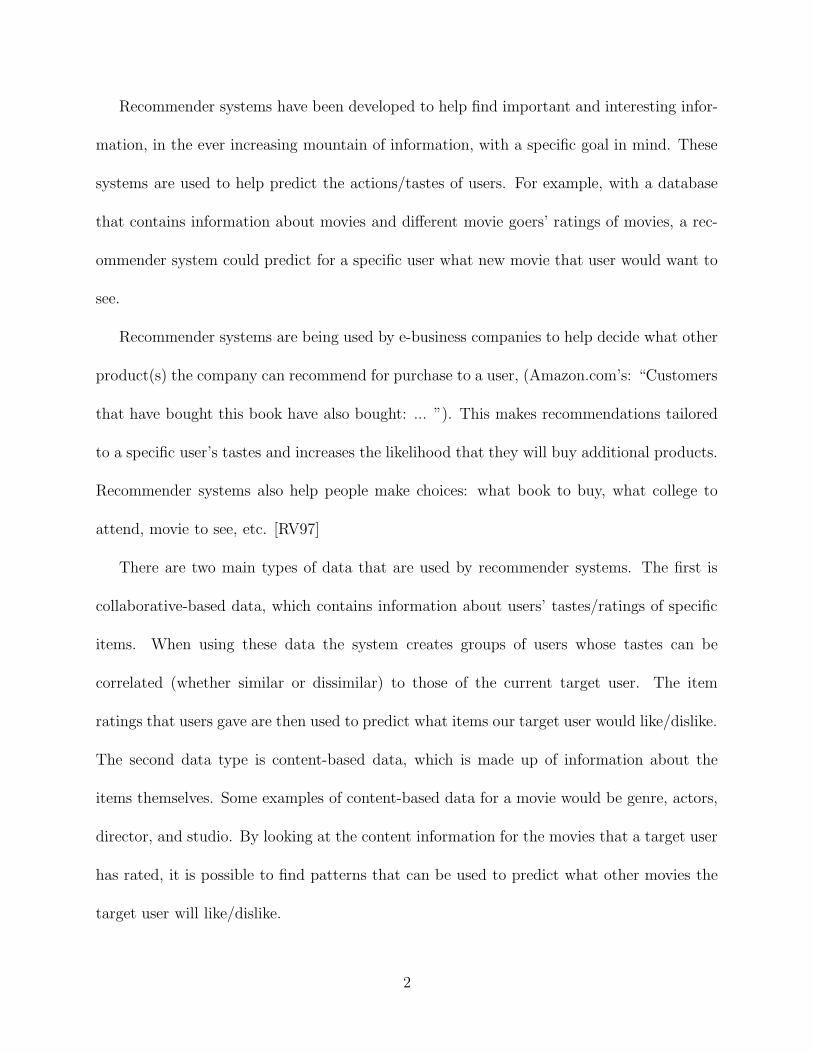
Recommender systems have been developed to help find important and interesting infor-
mation, in the ever increasing mountain of information, with a specific goal in mind. These
systems are used to help predict the actions/tastes of users. For example, with a database
that contains information about movies and different movie goers’ ratings of movies, a rec-
ommender system could predict for a specific user what new movie that user would want to
see.
Recommender systems are being used by e-business companies to help decide what other
product(s) the company can recommend for purchase to a user, (Amazon.com’s: “Customers
that have bought this book have also bought: ... ”). This makes recommendations tailored
to a specific user’s tastes and increases the likelihood that they will buy additional products.
Recommender systems also help people make choices: what book to buy, what college to
attend, movie to see, etc. [RV97]
There are two main types of data that are used by recommender systems. The first is
collaborative-based data, which contains information about users’ tastes/ratings of specific
items. When using these data the system creates groups of users whose tastes can be
correlated (whether similar or dissimilar) to those of the current target user. The item
ratings that users gave are then used to predict what items our target user would like/dislike.
The second data type is content-based data, which is made up of information about the
items themselves. Some examples of content-based data for a movie would be genre, actors,
director, and studio. By looking at the content information for the movies that a target user
has rated, it is possible to find patterns that can be used to predict what other movies the
target user will like/dislike.
2
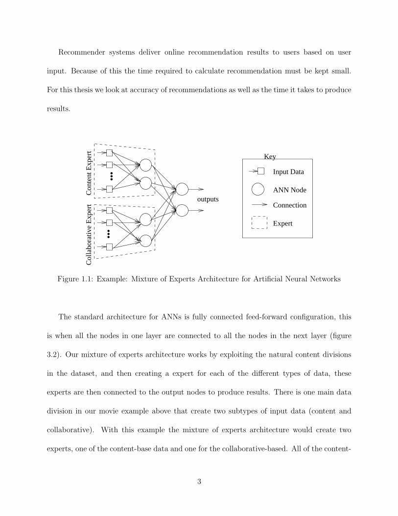
Recommender systems deliver online recommendation results to users based on user
input. Because of this the time required to calculate recommendation must be kept small.
For this thesis we look at accuracy of recommendations as well as the time it takes to produce
results.
...
...
Con
tent
Exp
ert
Expert
Connection
ANN Node
Input Data
Key
Col
labo
rativ
e E
xper
t
outputs
Figure 1.1: Example: Mixture of Experts Architecture for Artificial Neural Networks
The standard architecture for ANNs is fully connected feed-forward configuration, this
is when all the nodes in one layer are connected to all the nodes in the next layer (figure
3.2). Our mixture of experts architecture works by exploiting the natural content divisions
in the dataset, and then creating a expert for each of the different types of data, these
experts are then connected to the output nodes to produce results. There is one main data
division in our movie example above that create two subtypes of input data (content and
collaborative). With this example the mixture of experts architecture would create two
experts, one of the content-base data and one for the collaborative-based. All of the content-
3

based input data would connect to a group of hidden nodes that would be designated the
content-based expert, and likewise all of the collaborative-based input data would connect
to a set of hidden nodes that would be the collaborative-based expert (figure 1.1). The data
are propagated through the network following the connections (the arrows) and an output
value is produced. Splitting the content-base and collaborative-base information allow us
to greatly reduced the number of connections, which in turn reduces the amount of time it
takes to make a recommendation to our target user.
We have found through experimentation that the mixture of experts architecture reduces
the training time by approximately 40% compared to the fully connected architecture. Also,
mixture of experts achieves the same accuracy of the fully connected architecture, and has
only a 5% decrease in the precision values. We compared our work to the seminal work
of Billsus and Pazzani, as presented in [BP98]. We were able to achieve better accuracy
of recommendations than Billsus and Pazzani and comparable results when recommending
the top 3 and 10 movies to a target user. We achieved this without having to employ
dimensionality reduction techniques to pre-process the data as they did. Unlike Billsus and
Pazzani, we were able to obtain better recommendation accuracy and precision when using
both content and collaborative data over those obtained when using only collaborative data.
These results added upon the Billsus and Pazzani’s future work of attempting to create a
beneficial combination of content and collaborative data using neural networks.
4
Chapter 2
Background and Related Work
2.1 Neural Networks
Neural networks were originally introduced as a model of our brain (or at least the neurons
that make up the brain). This idea was originally proposed by N. Rashevsky in 1938 [Ras38]
and further developed by McCulloch and Pitts in 1943 [MP43]. The brain is composed of
neurons that when stimulated will fire or not fire based on the amount of stimulation received.
Neurons are connected to other neurons by synapses. When a neuron fires it causes some
action (whether it is stimulating another neuron or causing an end result, like moving your
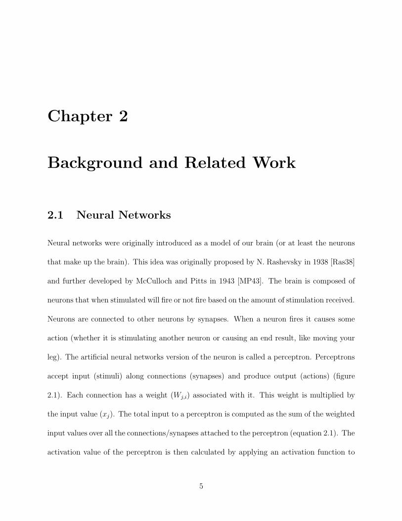
leg). The artificial neural networks version of the neuron is called a perceptron. Perceptrons
accept input (stimuli) along connections (synapses) and produce output (actions) (figure
2.1). Each connection has a weight (Wj,i) associated with it. This weight is multiplied by
the input value (xj). The total input to a perceptron is computed as the sum of the weighted
input values over all the connections/synapses attached to the perceptron (equation 2.1). The
activation value of the perceptron is then calculated by applying an activation function to
5

this sum of weighted inputs (equation 2.2). An activation function commonly used is the
sigmoid activation function. The sigmoid activation function like other activation functions
is nonlinear. The perceptron’s output (ai) is then propagated through the network in a
similar fashion.
.
.
.
inputs
output
O
WW
W
W01
2
n
kΣ
Figure 2.1: ANN node
xi =∑
j∈ in connections
Wj,ixj (2.1)
ai = σ(xi) =1
1 + e−xi
(2.2)
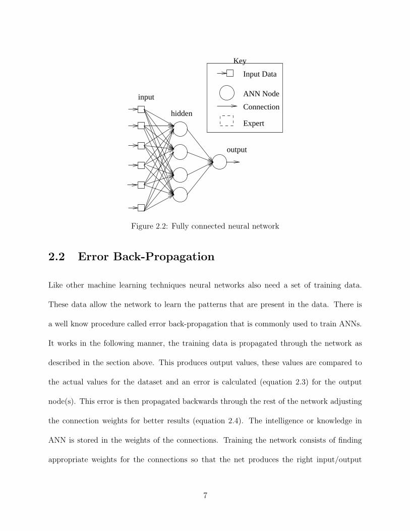
The fully connected network consists of three layers that are connected to each other.
The first layer is called the input layer. In this layer there is a node for each input value.
The second layer is called the hidden layer which consists of the middle set of nodes. In our
experiments we will only be using one hidden layer although it is possible to have many.
The last layer is the output layer, from which we get the results of the ANN. We construct
a feed-forward ANN in which all nodes are only connected to nodes in the next layer (figure
2.2). There are other types of ANN where it is allowed to have connections between any two
nodes in the network.
6
Expert
Connection
ANN Node
Input Data
Key
input
output
hidden
Figure 2.2: Fully connected neural network
2.2 Error Back-Propagation
Like other machine learning techniques neural networks also need a set of training data.
These data allow the network to learn the patterns that are present in the data. There is
a well know procedure called error back-propagation that is commonly used to train ANNs.
It works in the following manner, the training data is propagated through the network as
described in the section above. This produces output values, these values are compared to
the actual values for the dataset and an error is calculated (equation 2.3) for the output
node(s). This error is then propagated backwards through the rest of the network adjusting
the connection weights for better results (equation 2.4). The intelligence or knowledge in
ANN is stored in the weights of the connections. Training the network consists of finding
appropriate weights for the connections so that the net produces the right input/output
7

behavior dictated by the data. In equations 2.3 and 2.4, δk is the kth output node’s error. It
is calculated from ok the network’s predicted output value for that node and tk the desired
output value. Hidden nodes’ errors are calculated by taking the sum of all the weights (Wkh)
multiplied by the errors from the connecting output (δk) nodes, and then multiplying the
sum by the output of the hth hidden node (oh). The error back-propagation algorithm is an
implementation of a gradient descent search method. The error back-propagation algorithm
searches in the space of weights for the minimum of the mean squared error metric [Mit97].
δk = ok(1 − ok)(tk − ok) (2.3)
δh = oh(1 − oh)∑
k∈outputs
Wkh · δk (2.4)
There is one problem with the gradient descent algorithm, the local minimum problem.
In the gradient descent algorithm you traverse a space by taking a step in the direction that
looks the best at the current moment in hopes that you will find the best overall (or global)
position in that space. The algorithm stops searching when all possible next steps bring
you farther away from your goal (the lowest possible error). The local minimum problem
occurs when you have areas in your space that are a local minimum (the lowest in their
local neighborhood) but are not the lowest value in the whole space, so as you traverse the
space you can be drawn into a local minimum thinking that it is the global minimum. One
solution to this problem it using a decay the varies the size of the steps that are taken on
each iteration through the algorithm. This solves the problem by allowing you to step over
local minimums on the way to finding the global minimum. Because the size of the step
degrades as the number of iterations increases as you approach the true answer you will be
8

taking smaller steps to focus in on the exact answer.
2.3 Recommender Systems
When individual people and companies are faced with a problem or decision, it is com-
mon for them to try to find other information that will make the process easier. Some-
times a person will find a huge quantity of data. For example, when a student is trying
to pick a college, or a company is trying to make product recommendations to its clients.
It takes a lot of time and effort to sort through all of this information. Recommender
systems help make this process easier, by taking the gathered information and producing
recommendations to the user. Some examples of existing systems that do recommenda-
tion are WiseWire (www.wisewire.com), Content Advisor (www.contentadvisor.com), Gus-
tos (www.gustos.com), and GroupLens (www.cs.umn.edu/Research/GroupLens).
Recommender systems work by creating a model from the data and then using this
model to predict the desired results. With movie data, we could give the system information
about the content of the movies as well as what other people’s view and some of our own
movie ratings, and the system could produce recommendations about other movies that we
would like. How exactly the input data gets converted to recommendations is a large area
of research. Some examples can be found in [BS97], [BP98], [LAR02], and [RV97]. They
use techniques such as correlation, association rules, and neural networks. In this work
we will be looking how an adaptation of neural networks can convert the input data into
recommendations for the user.
Previous work using ANN-based recommender systems has mainly focused on using
9

collaborative-based information, with major work from Billsus and Pazzani [BP98]. In their
paper, they show how using singular value decomposition with ANNs produces a better rec-
ommender system than just a correlation method or decision tree approaches alone. singular
value decomposition (also known as principal components analysis) is a well-known linear al-
gebra dimensionality reduction technique that can be used to make sparse data more compact
[DJ99]. They tested their system with movie data from the EachMovie database [McJ97].
We used the same database so that we can compare our results with theirs.
The correlation approach models similarities between users. It does this by calculating
a vote for a instance by a weights sum of the votes other users gave this instance and the
target users rating [BR94]. Decision trees use an entropy measure to select the attributes
that will most quickly determine the classification. This is done by creating a hierarchical
tree structure. The attribute that has the lowest entropy over the training data is places at
the root of the tree, then for each attribute value pair of the root node a new entropy value
is calculated for all the other attributes. The lowest attribute to selected for each of the
roots attribute value pairs and this process continues until the entropy for all of the leaves
is 0 (so total classification is possible) or some small value if error is acceptable.
2.3.1 Content-based and Collaborative Recommendation
There generally two different types of data that are given to recommender systems, content-
based information and collaborative-based information.
Content-based information describes the actual data. In the movie domain content-
based data would be genre (comedy, horror, action ...), actors names, the year a movie
10
came out, whether it was in color or black and white, etc. If you are doing content-based
recommendation you will find patterns between the target user and the content. For example
you will find things like a particular target user likes movies that are comedies that don’t have
Jim Carrey but do have Tom Hanks. One of the down sides to content-based information is
that it is hard to find/extract the useful features from different domains.
Collaborative information contains other users opinions on the data, an example in the
same domain would be people’s ratings of movies. Recommender systems that just use
collaborative information will find correlations between the users in the system and the
target user. One of the down falls of many research efforts that just use collaborative-
based information is that they only find correlations between users that have rated things in
common. This is a problem when your database contains thousands of instances and a given
target user will only have rated a handful. Two users might have extremely correlated tastes
(the both like exactly the same movies or if one likes it the other hates it), but if they have
not rated any movies in common this commonality will not be found and could consequently
decrease the accuracy of the resulting recommendations. There are also existing systems
that attempt to combine content and collaborative information [BS97] and [Yu98].
2.4 Weka
In order to gather experimental results we have adapted Weka (version 3-2), a data min-
ing tool from the University of Waikato in New Zealand [FW00] and [F+02]. Weka is an
open source Java application. The Weka system contains some visualization, pre- and post-
processing tools as well as a suite of data mining algorithms for classification, clustering and
11
associations.
There are three main modes that Weka can run in: command line, experimenter GUI,
and explorer GUI. The command line has all the functionality that the GUIs provide, but
the GUI provides ease of use. The experimenter holds all of the visualization, pre- and
post- processing functionality as well as letting you run single experiments with any of the
mining algorithms. The explorer allows users to run sets of test with any of the classification
algorithms. The input data for this system is in an ARFF or database format. The ARFF
format is a text file that specifies the attributes and comma or tab separated data.
This system is extremely useful because of its wealth of functionality and the ability that
it give the user to implement new functions or change existing code to better suit his or her
purpose. There is also an active Weka email list on which you can ask other users for help
or make suggestions for future changes to the system.
The original Weka ANN architecture, allows you to specify: number of hidden nodes
and layers, momentum, learning rate, decay, validation set size and threshold, maximum
number of epochs, the random seed, whether or not you want to normalize the attributes
and the class. They also have an option that will let you see a graphical representation of
your network configuration. This implementation of ANNs produces a feed forward fully
connected architecture and uses the error back-propagation algorithm to train the network.
12

Chapter 3
A New ANN Architecture for
Recommender Systems
This chapter is broken up into two main sections. First, we describe the design of our
mixture of expert architecture, how it is constructed in ANNs and its impact when used in
a recommender system. Second, we describe the implementation of our system.
3.1 Network Architecture
In section 2.1 we described the standard fully connected architecture for neural networks.
Taking advantage of the natural division between collaborative and content data, we now
propose a different neural network architecture which we refer to by the name mixture of
experts. The mixture of experts architecture is depicted in figure 3.1. For comparison,
the fully connected architecture appears in figure 3.2. The mixture of experts architecture
creates groups of input nodes by data type. These groups of input nodes are each connected
to one group of hidden nodes (each group of hidden nodes becomes an expert for that data
13
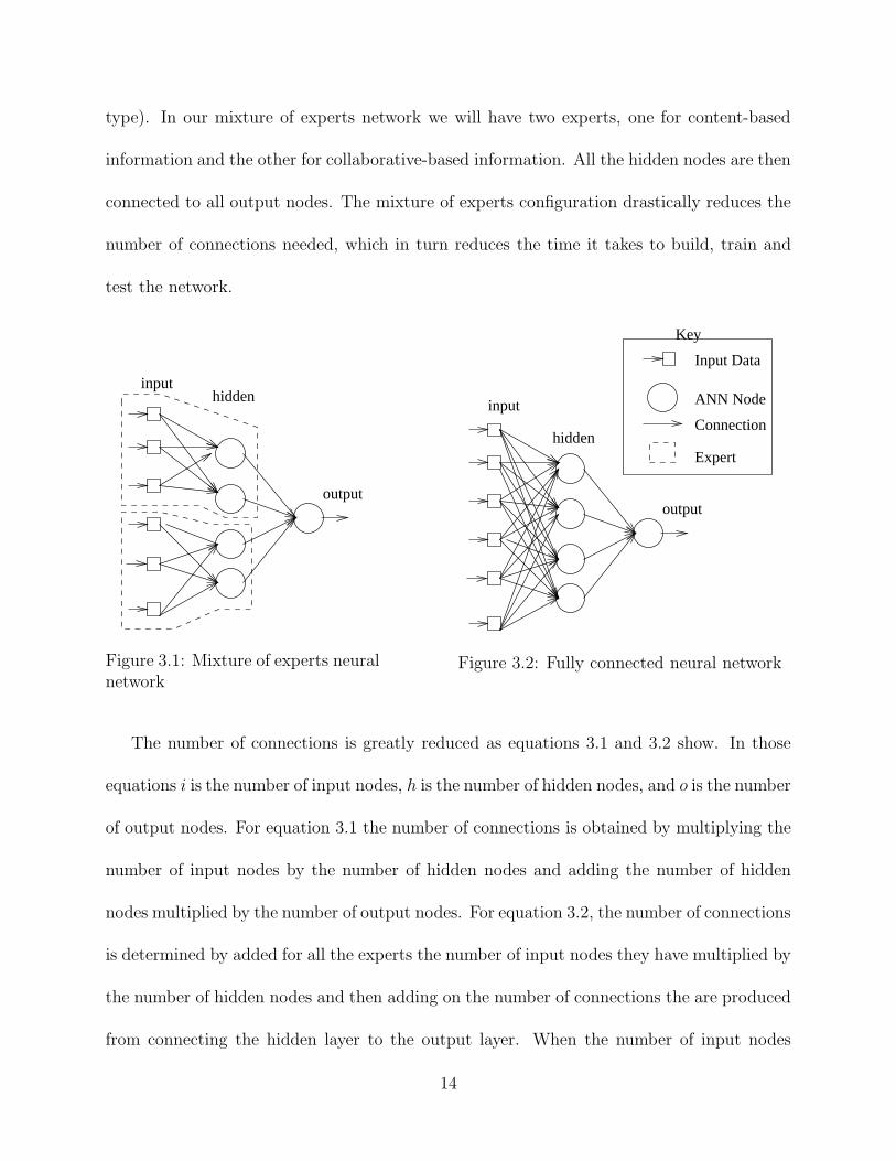
type). In our mixture of experts network we will have two experts, one for content-based
information and the other for collaborative-based information. All the hidden nodes are then
connected to all output nodes. The mixture of experts configuration drastically reduces the
number of connections needed, which in turn reduces the time it takes to build, train and
test the network.
output
inputhidden
Figure 3.1: Mixture of experts neuralnetwork
Expert
Connection
ANN Node
Input Data
Key
input
output
hidden
Figure 3.2: Fully connected neural network
The number of connections is greatly reduced as equations 3.1 and 3.2 show. In those
equations i is the number of input nodes, h is the number of hidden nodes, and o is the number
of output nodes. For equation 3.1 the number of connections is obtained by multiplying the
number of input nodes by the number of hidden nodes and adding the number of hidden
nodes multiplied by the number of output nodes. For equation 3.2, the number of connections
is determined by added for all the experts the number of input nodes they have multiplied by
the number of hidden nodes and then adding on the number of connections the are produced
from connecting the hidden layer to the output layer. When the number of input nodes
14
gets large the difference between the number of connections produced will increase. Also
the more hidden nodes you have the fewer connection the mixture of experts architecture
will have relative to the fully connected architecture. It is important to note that random
experts should not be defined just to reduce the number of connections. This is because the
weights on the connections hold the knowledge of the neural network, so when a connection
is randomly removed there is no guarantee that the neural network will be able to produce
the right output. An expert should only be added if a natural division in the data can
be found. For example if you take the movie domain, you can have data on user ratings
of movies (collaborative information) and descriptive information about the movie (content
information), this would give you two experts (one for collaborative and one for content
information). You would not want to split the collaborative users into two different experts
because then you are limiting the influence that different collaborative users can have.
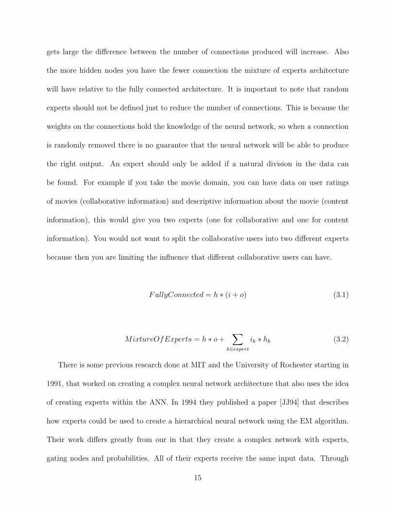
FullyConnected = h ∗ (i + o) (3.1)
MixtureOfExperts = h ∗ o +∑
k∈expert
ik ∗ hk (3.2)
There is some previous research done at MIT and the University of Rochester starting in
1991, that worked on creating a complex neural network architecture that also uses the idea
of creating experts within the ANN. In 1994 they published a paper [JJ94] that describes
how experts could be used to create a hierarchical neural network using the EM algorithm.
Their work differs greatly from our in that they create a complex network with experts,
gating nodes and probabilities. All of their experts receive the same input data. Through
15

training and use of the gating networks experts will focus on one area or aspect in the data.
With their algorithm there is no distinct separation between what data each of the experts
can cover, they calls this “soft” split of data. Our mixture of network architecture uses a
“hard” split of the data more like CART [OS84], MARS [Fri90] and ID3 [Qui86], where
overlap between data splits are not allowed. Their hierarchical mixture of experts reduces
neural network error very quickly, but their network is very large compared to ours. With
only 12 input nodes the equivalent of 60 hidden nodes are used in 4 different hidden layers.
With our mixture of experts architecture we use a little over 2000 input nodes and only 1
hidden layer with 4 hidden nodes and achieve a high quality of recommendations.
3.2 Recommender System
The job of the mixture of experts architecture is to fill the black box in recommender systems
that takes in the input data and produces recommendations to the user. Our architecture
does a better job than the standard fully connected ANN model when there is a natural
division in the data. It does this by producing results faster without reducing the quality of
the recommendations.
After construction of the mixture of experts architecture, a recommender system that
uses this method will do testing and training just like any other recommender system. The
mixture of experts architecture will take in the different types of data and, as specified
by the user, will construct a neural network with the correct number of experts. Next,
the recommender system will train over the training portion of the input data. When the
training is completed, new unseen test data instances will be pushed through the neural
16
network and the mixture of experts architecture will produce a classification for each of the
instances. If the network classifies an instance as the type we want to recommend (i.e. we
want to recommend movies that the use will like, not dislike) then the score (in our case the
ANN output value) is stored. After all the testing instances have been pushed through the
ANN, the recommender system sorts the instances by their scores and recommends the top
instances to the user.
To our knowledge, although research has been done involving ANN and recommender
systems [BP98], no one has looked into using a mixture of experts architecture in this context.
We show in this next chapter that this new architecture makes similarly accurate predictions
to the fully connected architecture, in less time. This contributes greatly in an area of
research where it is important to get high quality recommendations to the user in real time.
3.3 Implementation in Weka
Weka version 3-2 comes with an standard feed-forward implementation of ANN that allows
you to do cross-validation, validation, vary the number of epochs, the random seed, as well
as several other parameters (see section 4.1.3 for discussion of these techniques). Because of
all the features that Weka already provided, we decided to adapt their version so that it was
possible to create mixture of experts architectures rather than implementing the architecture
from scratch.
17

3.3.1 ANN Code Modifications
We modified Weka’s neural network code to accept an optional string that if given would
describe how the user wanted to split up the input data into experts and also designate how
many hidden nodes should be allocated to each of of the experts. The format follows from
3.3, where xi designates the number of contiguous inputs for the ith expert and hi represents
how many hidden nodes the xi inputs should connect to. This string was then read into the
system and connections were setup accordingly. For example: [1000,2][36,3] would create
two experts, the first would use the first 1000 inputs into the ANN and 2 hidden nodes, and
the second would use the next 36 inputs and 3 hidden nodes.
[x0, h0][x1, h1]...[xn, hn] (3.3)
The mixture of experts string can be passed into the system as run time as a command
or GUI option. If the string length was zero then the ANN code would create a fully
connected architecture with the specified number of hidden nodes. Code was added to deal
with creating the correct connections if the mixture of experts string was present. The code
does the following: it extracts the next expert from the string ([y,n]) for the next y inputs
would be connected to the next unused n hidden nodes. This would loop until all of the
experts were read off the string. Then all of the hidden nodes would be connected to the
output nodes. If the user specified that there would be more inputs or hidden nodes than
were actually present an error message would be sent to the screen. One of the drawbacks of
this implementation is that one cannot have multiple hidden layers or overlapping experts.
18

3.3.2 Output Measures Added
We also added several performance measures that would be outputed during experimenta-
tion. The average number of epochs used during training by a target user, accuracy, and the
top n precision. Top n precision, is the precision value for the top n raked recommendations
for a given target user. This metric provides a way to measure the correctness of the top
recommendations. This was calculated by counting the n instances with the highest ANN
output value that was above some predefined threshold. We then took the percentage of
those recommended.
3.3.3 Input Data and Experts
Weka’s implementation of neural networks creates one output node for each of the possible
nominal values of the classification attribute. In our case, the class value represented whether
the target user liked or disliked a specific movie. So, ANNs were created with 2 output nodes,
one that classified for liking a movie and the other that classified for disliking a movie (figure
1.1). When we used the mixture of experts architecture 2 experts were created, one for
collaborative-based data and one for content-based data.
19

Chapter 4
Experimental Protocol and Evaluation
This chapter explains the protocol we used to evaluate our new mixture of experts archi-
tecture. First we present the dataset used and some measures for evaluating our system’s
performance. Then we present and analyze the results of our experimentation. This analysis
includes comparisons between the mixture of experts and fully connected ANNs architectures
and comparisons of our results with those from Billsus’ and Pazzani’s work [BP98].
4.1 Protocol
4.1.1 Data
We have run experiments with data from the EachMovie database [McJ97]. The Each-
Movie database contains information about users’ movie ratings (our collaborative-based
information) and genre (our content-based information). We selected the first 1000 users as
collaborative users that had rated more than 100 movies. The target users were selected
from the users who’s id was over 70000 ( so that the collaborative group and the test group
20

of users are disjoint) and had also rated approximately 50 movies.
Because the EachMovie database only contains 10 content attributes we have also gather
content information from MovieLens database developed by GroupLens [Gro] and the In-
ternet Movie Database (IMDB) [Inc02]. This increased the number of content attributes to
36 with 1100 attribute value pairs, making the number of collaborative inputs and content
inputs almost the same. However, content data are only available for 430 out of 999 movies
that are present in our EachMovie dataset.
Dataset Num. of Num. of Num. of Total % Avg. Num. of Non-
Collab. Content Attr. Val. Pairs Missing Missing Val. per Inst.
EachMovie 1000 10 1010 96.001% 80.419
MovieLens 1000 36 2100 96.298% 75.417
Even though there is a large number of attributes and attribute value pairs for these
datasets, only approximately 4% of data values are present in this dataset and the rest of
the data is missing. This means that on average there are only about 75 to 80 values per
instance out of 1010 or 2100 depending on the dataset. This sparseness of the data will make
generating recommendation extremely hard.
The latter part of this chapter contains a series of graphs that display the results of our
experimentation. The following notation is used to depict the number of experts used and
hidden nodes that each expert uses: [n] and [y][z]. The first one, [n], denotes a unique
expert with n hidden nodes. The second one [y][z] denotes two experts, the first expert has
y hidden nodes and the second expert has z hidden nodes. For example [4] would denote a
fully connected architecture with 4 hidden nodes and [2][2] would denote a mixture of experts
21

architecture with two hidden nodes for content and two for collaborative. We can use this
notation without specifying the number of inputs given to an expert because each experiment
has a well-defined number of content and collaborative inputs, so they are omitted in this
notation.
4.1.2 Performance Measures
There are several metrics commonly used in evaluating recommender systems. We will be
using precision and recall along with the time needed to build a neural network to evaluate
the different network architectures.
Precision is the percentage of correctly recommended items out of the total number of
recommended items (equation 4.1). Accuracy is the number of correctly classified items
divided by the number of classified items (equation 4.2).
System PredictionLike Dislike
True+ False- Like ActualFalse+ True- Dislike User Ratings
Figure 4.1: Confusion Matrix
Figure 4.1 is a confusion matrix, the columns represent the systems prediction (of like
or dislike of a movie) and the rows represent the actual user rating. The confusion matrix
keeps track of how many test items were correctly and incorrectly classified for a given target
user. For example if the system predicted that a target user would like a movie and the user
actually did, the number of true positives would be incremented. Likewise if the system
predicted that the target user would dislike a movie and the user actually like it than the
22

number of false negatives would be incremented. A confusion matrix is calculated for each of
the target users over the testing dataset, is then used to calculate the precision and accuracy
values for that target user.
Precision =number of true positives
number of true positives + number of false positives(4.1)
Accuracy =number of true positives + number of true negatives
number of test instances in the dataset(4.2)
For our experiments we would like high precision and high accuracy. Most of the target
users in our dataset have rated more movies as dislike than like, which provides us with
more data to help us classify when a target user will not like a movie. From this we expect
that our experiments will produce higher accuracy than precision, because precision is only
concerned with predicting movies that the target user will like, and accuracy is concerned
with classifying both likes and dislikes.
Finally, measuring the time allocated to build the model will allow us to compare how
much time is gained by eliminating connections in the network and how this affects the
precision and accuracy.
Billsus and Pazzani also show the top n precision value for all their target users. The top
n precision is defined as taking the best n recommendations and calculating their precision if
the recommendation value is above some predefined threshold. For example, after performing
training we input our test data and we get the following ordered top 5 results:
23
Movie Predicted Score User Rating
Big 0.9 Like
Dead Poet’s Society 0.8 Dislike
Crimson Tide 0.8 Like
The One 0.75 Like
Babe 0.5 Dislike
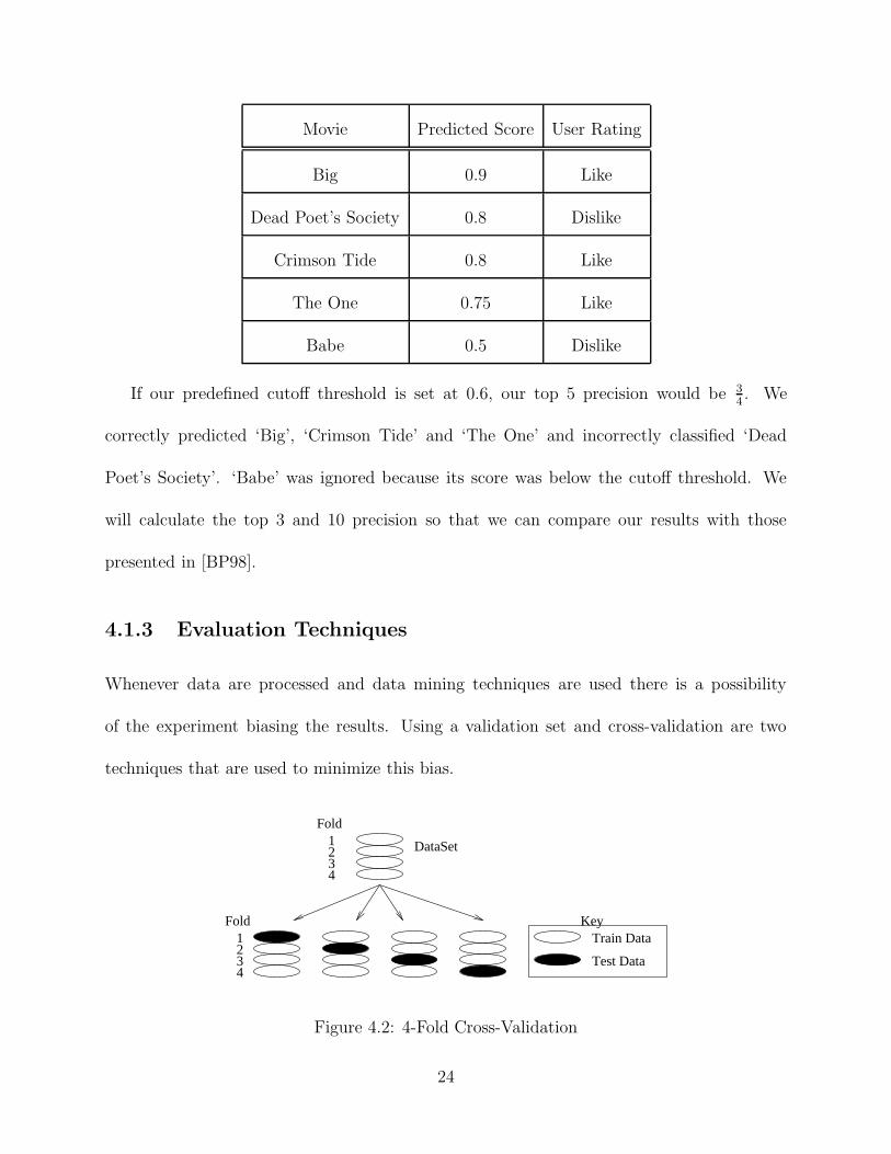
If our predefined cutoff threshold is set at 0.6, our top 5 precision would be 3
4. We
correctly predicted ‘Big’, ‘Crimson Tide’ and ‘The One’ and incorrectly classified ‘Dead
Poet’s Society’. ‘Babe’ was ignored because its score was below the cutoff threshold. We
will calculate the top 3 and 10 precision so that we can compare our results with those
presented in [BP98].
4.1.3 Evaluation Techniques
Whenever data are processed and data mining techniques are used there is a possibility
of the experiment biasing the results. Using a validation set and cross-validation are two
techniques that are used to minimize this bias.
1234
1234
Test Data
Train DataKey
DataSet
Fold
Fold
Figure 4.2: 4-Fold Cross-Validation
24

Cross-validation eliminates bias by creating n-folds (or sections) in the dataset and pro-
ducing results that are the average of the testing results across all fold. For this thesis we are
using 4-fold cross-validation. Our dataset is randomly broken into 4 sections. Evaluation is
repeated 4 times, each one with a different fold used as the test section while the remaining 3
sections are used as the training data (figure 4.2). The results of each test are then averaged
together to get the desired metric values. This makes sure that one produces reliable results,
by reducing the bias that could occur if one only tested over one section of the data only.
On the other hand, using a validation set reduces the probability of over-fitting the
constructed model to the data. When using a validation set, a percentage of the training
dataset is used to check if the accuracy of a partially trained ANN is still improving during
the training process. This is done by training one iteration over the training data minus the
validation set and then using the validation set to calculate the system’s error. On the next
training iteration the old error is compared to the new system’s error. If the error increases
during each of a predefined number of consecutive iterations, or some error level is reached
then the training is stopped.
4.2 Tuning Our System
Through our experiments we show that a mixture of experts approach gives an advantage
over the normal network configuration. We performed several different experiments in order
to gather reliable results.
25

4.2.1 Initial Test and Parameter Settings
After modifying Weka so that it could construct a mixture of experts architecture, we wanted
to test our architecture to see if it would work in a simple case. To do this we began by
gathering content and collaborative data for one user (user id 9030). For this initial test
we used 10 content-based attributes from the EachMovie database, although we added more
in later experiments. We then ran several experiments playing with different parameters to
find the best combination.
Parameters to be Set:
• Collaborative Group Size
• Maximum Number of Epochs
• Validation Set size
We ran the experiments with four hidden nodes (for mixture of experts 2 hidden nodes
for collaborative and 2 hidden nodes for content) and calculated both the precision for target
users liking and disliking movies. We varied the collaborative group size (figure 4.3), and the
number of epochs (figure 4.5). We also looked at the time it took to build the network (figure
4.4) and how different validation set sizes effected the results (figure 4.6). Precision values
were calculated using confusion matrixes (figure 4.1) generated during testing. Equation 4.1
shows the formula for calculating the precision for movies predicted to be liked by the user.
The equation for the precision of movies predicted to be disliked by the target user is the
number of true negatives divided by the sum of false negatives and true negatives.
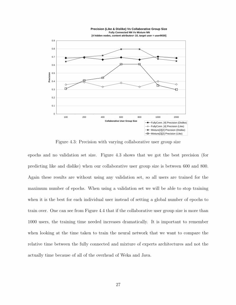
Experiments displayed in figures 4.3 and 4.4 helped us to determine how many many
collaborative users we should use. These experiments were run with a maximum of 500
26
Precision (Like & Dislike) Vs Collaborative Group Size Fully Connected NN Vs Mixture NN
[4 hidden nodes, content attributes= 10, target user = user9030]
0
0.1
0.2
0.3
0.4
0.5
0.6
0.7
0.8
0.9
100 200 400 600 800 1000 2000
Collaborative User Group Size
Pre
cisi
on
FullyConn. [4] Precision (Dislike)
FullyConn. [4] Precision (Like)
Mixture[2][2] Precision (Dislike)
Mixture[2][2] Precision (Like)
Figure 4.3: Precision with varying collaborative user group size
epochs and no validation set size. Figure 4.3 shows that we got the best precision (for
predicting like and dislike) when our collaborative user group size is between 600 and 800.
Again these results are without using any validation set, so all users are trained for the
maximum number of epochs. When using a validation set we will be able to stop training
when it is the best for each individual user instead of setting a global number of epochs to
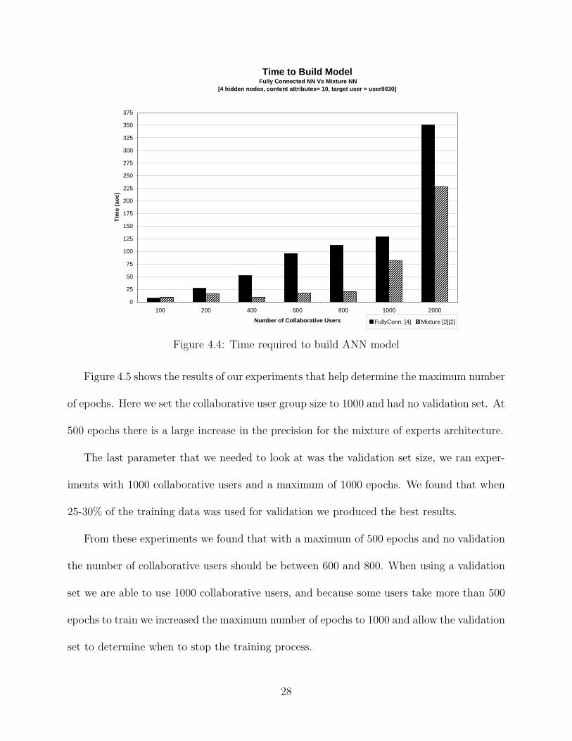
train over. One can see from Figure 4.4 that if the collaborative user group size is more than
1000 users, the training time needed increases dramatically. It is important to remember
when looking at the time taken to train the neural network that we want to compare the
relative time between the fully connected and mixture of experts architectures and not the
actually time because of all of the overhead of Weka and Java.
27
Time to Build Model Fully Connected NN Vs Mixture NN
[4 hidden nodes, content attributes= 10, target user = user9030]
0
25
50
75
100
125
150
175
200
225
250
275
300
325
350
375
100 200 400 600 800 1000 2000
Number of Collaborative Users
Tim
e (s
ec)
FullyConn. [4] Mixture [2][2]
Figure 4.4: Time required to build ANN model
Figure 4.5 shows the results of our experiments that help determine the maximum number
of epochs. Here we set the collaborative user group size to 1000 and had no validation set. At
500 epochs there is a large increase in the precision for the mixture of experts architecture.
The last parameter that we needed to look at was the validation set size, we ran exper-
iments with 1000 collaborative users and a maximum of 1000 epochs. We found that when
25-30% of the training data was used for validation we produced the best results.
From these experiments we found that with a maximum of 500 epochs and no validation
the number of collaborative users should be between 600 and 800. When using a validation
set we are able to use 1000 collaborative users, and because some users take more than 500
epochs to train we increased the maximum number of epochs to 1000 and allow the validation
set to determine when to stop the training process.
28

Parameter Value
Collaborative Group Size 1000
Maximum Number of Epochs 1000
Validation Set size 30%
As the result of this preliminary experimentation, the following parameters were selected:
1000 collaborative users, 30% validation set size, and 1000 epochs.
Precision (Like & Dislike) Vs Epochs Fully Connected NN Vs Mixture NN
[4 hidden nodes, content attributes= 10, collaborative attr. = 600 target user = user9030]
0
0.1
0.2
0.3
0.4
0.5
0.6
0.7
0.8
0.9
100 300 500 700 900 1100
Epochs
Pre
cisi
on
FullyConn. [4] Precision (Dislike)
FullyConn. [4] Precision (like)
Mixture[2][2] Precision (Dislike)
Mixture[2][2] Precision (like)
Figure 4.5: Precision for varying number of epochs
4.3 Evaluation of Our System
After determining values for the parameters, we ran a series of experiments described in
the table below to further validate our initial findings. This table is broken up by dataset
29
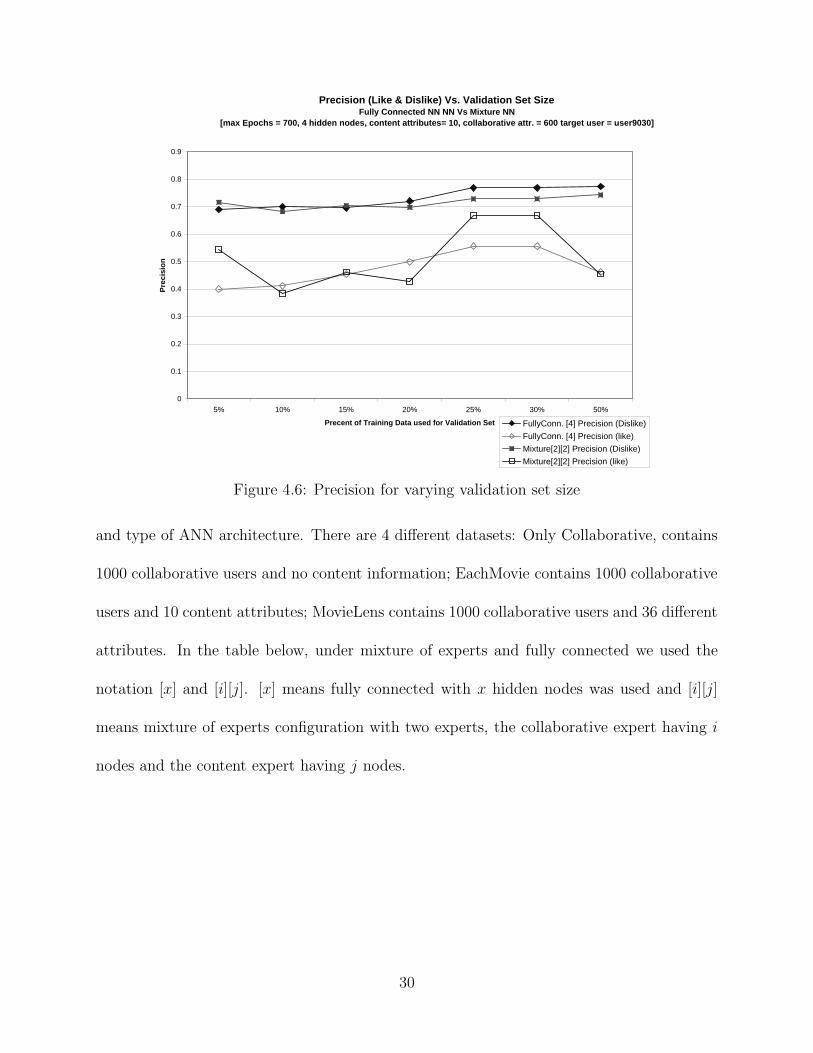
Precision (Like & Dislike) Vs. Validation Set SizeFully Connected NN NN Vs Mixture NN
[max Epochs = 700, 4 hidden nodes, content attributes= 10, collaborative attr. = 600 target user = user9030]
0
0.1
0.2
0.3
0.4
0.5
0.6
0.7
0.8
0.9
5% 10% 15% 20% 25% 30% 50%
Precent of Training Data used for Validation Set
Pre
cisi
on
FullyConn. [4] Precision (Dislike)
FullyConn. [4] Precision (like)
Mixture[2][2] Precision (Dislike)
Mixture[2][2] Precision (like)
Figure 4.6: Precision for varying validation set size
and type of ANN architecture. There are 4 different datasets: Only Collaborative, contains
1000 collaborative users and no content information; EachMovie contains 1000 collaborative
users and 10 content attributes; MovieLens contains 1000 collaborative users and 36 different
attributes. In the table below, under mixture of experts and fully connected we used the
notation [x] and [i][j]. [x] means fully connected with x hidden nodes was used and [i][j]
means mixture of experts configuration with two experts, the collaborative expert having i
nodes and the content expert having j nodes.
30

Dataset Mixture Of Experts Fully Connected
[2][2] [1][1] [4] [2] [1]
Only Collaborative yes yes yes yes yes
EachMovie yes yes yes yes yes
MovieLens yes yes yes yes yes
The following sections have the results from all of these different experiments as well as
how our results compared to those presented in the Billsus and Pazzani paper [BP98].
4.3.1 Increasing the Number of Target Users
We extended our experiments to cover 100 different target users. We also checked to make
sure that the random seed value does not influence the results. Experiments in the following
sections were ran with 4 hidden node configurations and also with 2 hidden nodes (mixture
of experts 1 node for content and 1 node for collaborative).
The 4-fold cross validation results gave us a very slightly worse precision for the mixture
of experts (0.5875 vs. 0.611) than the fully connected architecture (figure 4.7), although
this is a statistically significant difference the actual difference is not large (5%). Mixture of
experts completes 14.724 sec faster (19.516 sec for mixture of experts and 34.24 sec for the
fully connected model) (figure 4.7). Although we were hoping for better precision produced
in less time having about the same precision in 43% less time than the fully connected
configuration is still a great advantage.
To test the random seed values we selected 7 different random seeds and ran the same
experiment with each of the seed values. We found that the random seed value did not affect
31
Precision Vs Training Time
0
0.1
0.2
0.3
0.4
0.5
0.6
0.7
0.8
0.9
1
0 10 20 30 40 50 60 70 80 90 100 110 120 130 140 150 160 170 180 190
Training Time (sec)
Pre
cisi
on
Mixture of Experts Fully Connected
Average Fully ConnectedPrecision (0.611)
Average Mixture of ExpertsPrecision (0.5875)
Average Fully ConnectedTraining Time (34.24)
Average Mixture of ExpertsTraining Time (19.516)
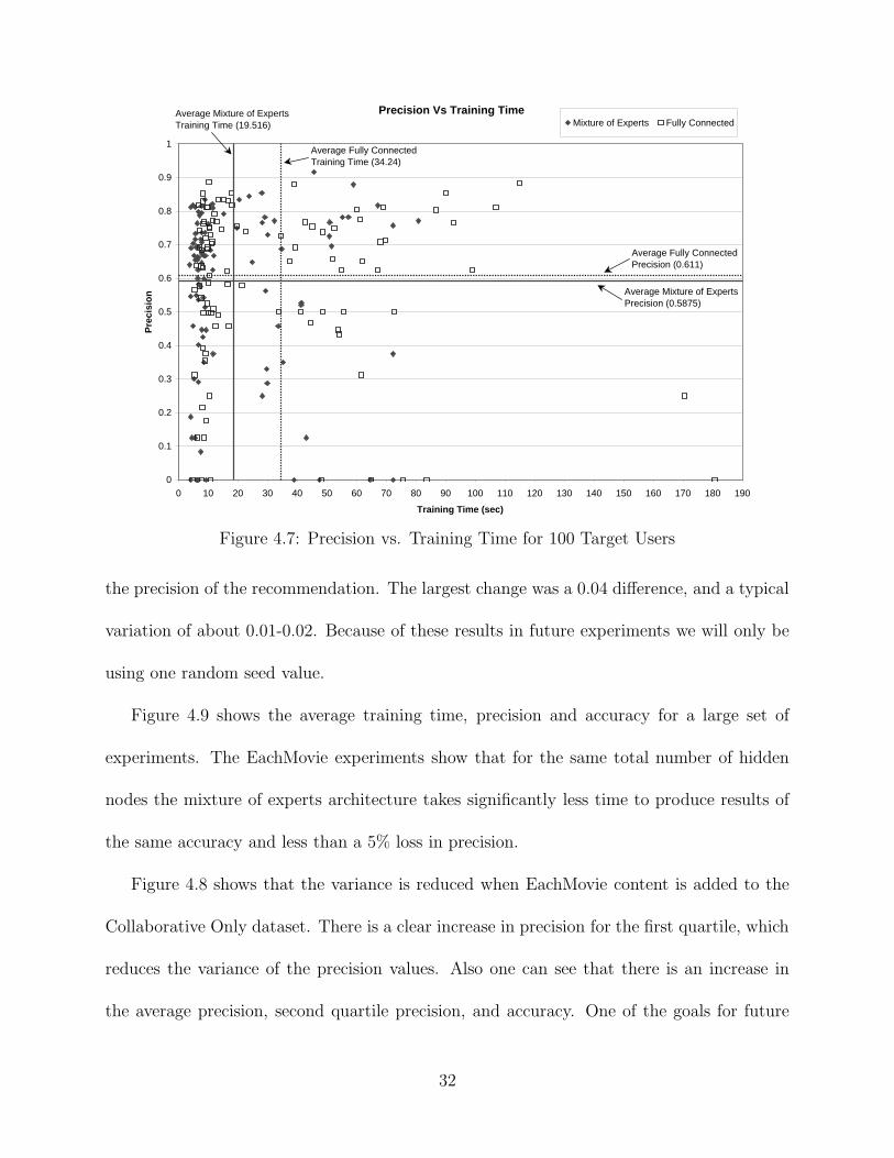
Figure 4.7: Precision vs. Training Time for 100 Target Users
the precision of the recommendation. The largest change was a 0.04 difference, and a typical
variation of about 0.01-0.02. Because of these results in future experiments we will only be
using one random seed value.
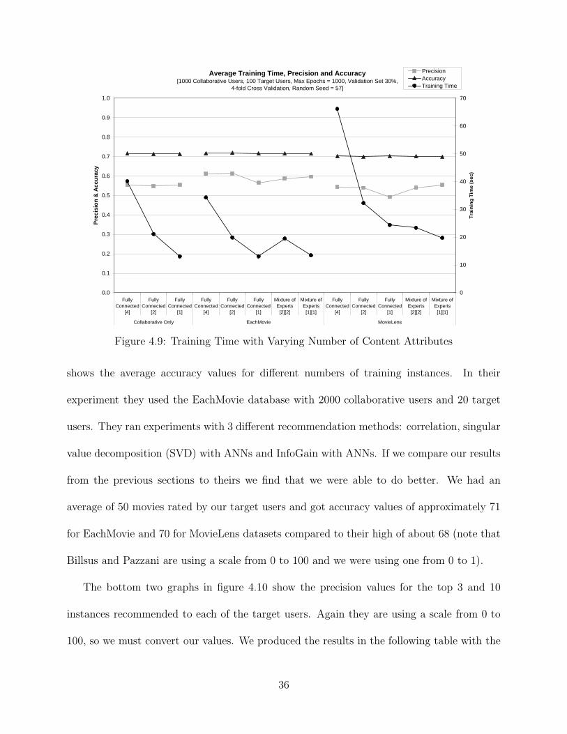
Figure 4.9 shows the average training time, precision and accuracy for a large set of
experiments. The EachMovie experiments show that for the same total number of hidden
nodes the mixture of experts architecture takes significantly less time to produce results of
the same accuracy and less than a 5% loss in precision.
Figure 4.8 shows that the variance is reduced when EachMovie content is added to the
Collaborative Only dataset. There is a clear increase in precision for the first quartile, which
reduces the variance of the precision values. Also one can see that there is an increase in
the average precision, second quartile precision, and accuracy. One of the goals for future
32

work suggested in [BP98] was to develop a neural network method for use in recommender
systems that would produce better results when both content and collaborative input data
are used. We have shown that the mixture of experts architecture accomplishes this goal,
when there is content data for all of the data instances.
4.3.2 Adding More Content-Based Information
In our previous experiments there were 1000 collaborative data points and only 10 content
data points for each tuple. We would like to increase the number of content data points
so that there is enough information to create two strong experts. Instead of one strong
and one weak expert. We also ran some experiments with no content data to complete our
comparison.
We have selected data from the GroupLens’ MovieLens database [Gro] as well as gathering
extra information from the Internet Movie Database [Inc02]. This gave us 36 different
attributes with a range of 2 to 236 values for a given attribute. Making the total number
of attribute values pairs 1100. Even through the number of attribute value pairs is very
large a sparse dataset is produced (96% of the data is missing values). This content for the
MovieLens dataset only covers approximately 430 movies in our database of 999 movies.
Adding MovieLens Content-Based Attributes
By replacing the content from our original dataset with the data from GroupLens we were
able to slightly increase the precision results for the third quartile and maximum precision
value (figure 4.8), however the average precision results decreased 8.1% for mixture of experts
and 11.1% for fully connected. This seems like a large loss of precision but in fact it is not,
33

since the average user has rated about 49.6 movies, 20.3 as like and 29.27 as dislike, and we
are only recommending one less movie to the user (the average for the number of movies
recommended by the fully connected architecture decreases from 12.4 to 11.03 movies, and
the corresponding average for the mixture of experts architecture decreases from 11.93 to
10.95 movies). This loss in precision could have been caused by the number of movies
without any content-based information. The accuracy that was produced (figure 4.9) stayed
almost constant between the mixture of experts and fully connected architectures for the
same dataset. There was a 2% decrease in precision between the EachMovie dataset and the
MovieLens dataset (accuracy values of 0.715 and 0.703 respectively).
When we compare the precision results for the different architectures of the MovieLens
data we can see that the mixture of experts does do slightly better (about 1-2%) than the
fully connected architecture depending on whether 4 or 2 hidden nodes are used. The big
difference is in the time that it takes to train the neural network. For 4 hidden nodes,
mixture of experts took 35.27% less time than the fully connected architecture, and with 2
hidden nodes mixture of experts took 38.75% less time. These results are expected if you
look at the calculations for the number of connections (equation 4.3 for fully connected; 4.4
for mixture of experts). There are 49.952% fewer connections for the mixture of experts
architecture.
ConnectionsFullyConnected = 2100 ∗ 4 + 4 ∗ 2 = 8408 (4.3)
ConnectionsMixtureExperts = 1000 ∗ 2 + 1100 ∗ 2 + 4 ∗ 2 = 4208 (4.4)
34

These results show that there was no statistically significant difference, between the
mixture of experts and the fully connected architectures, in accuracy or precision with the
MovieLens dataset even though the training time was significantly decreased when using the
same number of hidden nodes.
Precision Values for Mixture of Experts Vs Fully Connected[1000 Collaborative Users, 100 Target Users, Max Epochs = 1000, Validation Set 30%,
4-fold Cross Validation, Random Seed = 57]
0.0
0.1
0.2
0.3
0.4
0.5
0.6
0.7
0.8
0.9
1.0
FullyConnected
[4]
FullyConnected
[2]
FullyConnected
[4]
FullyConnected
[2]
Mixture ofExperts
[2][2]
Mixture ofExperts
[1][1]
FullyConnected
[4]
FullyConnected
[2]
Mixture ofExperts
[2][2]
Mixture ofExperts
[1][1]
Collaborative Only EachMovie MovieLens
Pre
cisi
on
Q1 MinMax Q3Average Q2Accuracy
Figure 4.8: Precision values for different datasets
4.3.3 Results
So far we have compared our new mixture of experts architecture with the fully connected
architecture and found that we are able to reduce the amount of time that it takes to make
a recommendation to the target user while keeping approximately the same precision. Next
we will compare our results to the results found in the Billsus and Pazzani paper [BP98].
The first thing that we will compare is the top left graph in figure 4.10, this graph
35
Average Training Time, Precision and Accuracy[1000 Collaborative Users, 100 Target Users, Max Epochs = 1000, Validation Set 30%,
4-fold Cross Validation, Random Seed = 57]
0.0
0.1
0.2
0.3
0.4
0.5
0.6
0.7
0.8
0.9
1.0
FullyConnected
[4]
FullyConnected
[2]
FullyConnected
[1]
FullyConnected
[4]
FullyConnected
[2]
FullyConnected
[1]
Mixture ofExperts
[2][2]
Mixture ofExperts
[1][1]
FullyConnected
[4]
FullyConnected
[2]
FullyConnected
[1]
Mixture ofExperts
[2][2]
Mixture ofExperts
[1][1]
Collaborative Only EachMovie MovieLens
Pre
cisi
on
& A
ccu
racy
0
10
20
30
40
50
60
70
Tra
inin
g T
ime
(sec
)
PrecisionAccuracyTraining Time
Figure 4.9: Training Time with Varying Number of Content Attributes
shows the average accuracy values for different numbers of training instances. In their
experiment they used the EachMovie database with 2000 collaborative users and 20 target
users. They ran experiments with 3 different recommendation methods: correlation, singular
value decomposition (SVD) with ANNs and InfoGain with ANNs. If we compare our results
from the previous sections to theirs we find that we were able to do better. We had an
average of 50 movies rated by our target users and got accuracy values of approximately 71
for EachMovie and 70 for MovieLens datasets compared to their high of about 68 (note that
Billsus and Pazzani are using a scale from 0 to 100 and we were using one from 0 to 1).
The bottom two graphs in figure 4.10 show the precision values for the top 3 and 10
instances recommended to each of the target users. Again they are using a scale from 0 to
100, so we must convert our values. We produced the results in the following table with the
36
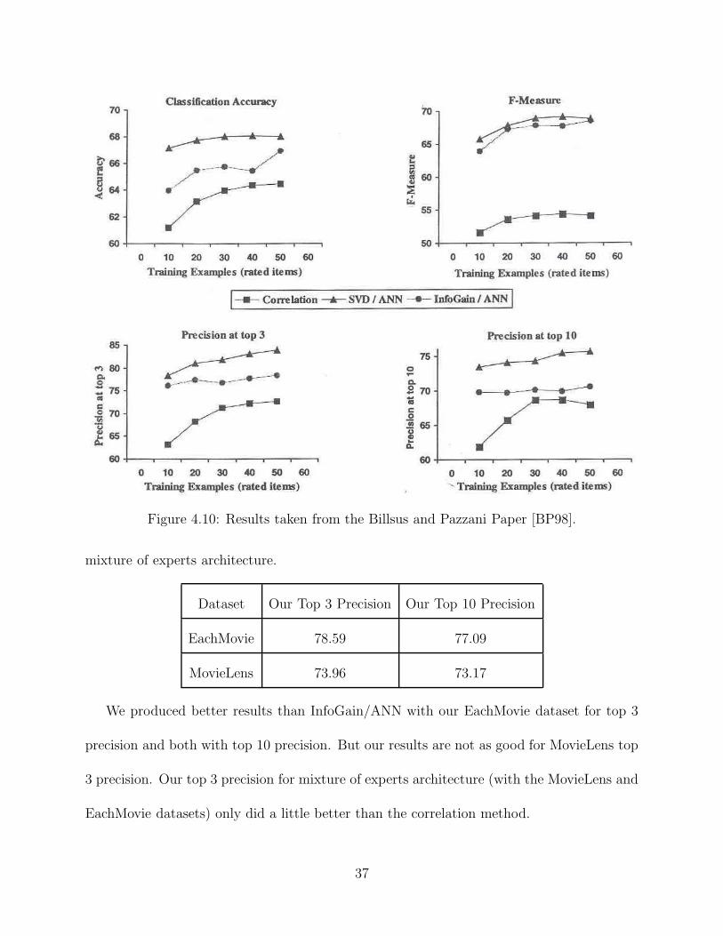
Figure 4.10: Results taken from the Billsus and Pazzani Paper [BP98].
mixture of experts architecture.
Dataset Our Top 3 Precision Our Top 10 Precision
EachMovie 78.59 77.09
MovieLens 73.96 73.17
We produced better results than InfoGain/ANN with our EachMovie dataset for top 3
precision and both with top 10 precision. But our results are not as good for MovieLens top
3 precision. Our top 3 precision for mixture of experts architecture (with the MovieLens and
EachMovie datasets) only did a little better than the correlation method.
37
Chapter 5
Conclusions
The main contribution of this work is the creation of a new architecture for neural networks.
The mixture of experts architecture successfully reduces the amount of time required to train
an ANN, when a natural division is present in the input data, without reducing the accuracy
of results. This is accomplished by decreasing the number of connections between the input
and hidden layers of the neural network. Connections are reduced by creating clusters of
input nodes and hidden nodes to form an expert, and only making connections between
input and hidden nodes in the same cluster.
This architecture is extremely useful in recommender systems where recommendations
need to be computed and presented to the user in real time. Besides from being a domain
where time performance is important, recommender system research has identified two main
types of input data, content-based and collaborative-based information. This type of domain
makes an excellent testbed for our mixture of experts architecture.
We implemented a Java version of our mixture of experts architecture for neural networks
in the Weka system [F+02]. Using this program we performed a series of experiments using
38

data from the EachMovie database and additional information from the MovieLens and
Internet Movie Databases. In order to make recommendations to our target users, we trained
an ANN for each target user using a portion of the dataset, allowing thereby the ANN to
learn the taste of the target user. Next we tested our trained neural network, by passing a
set of test data through the ANN which produced predictions about which movies the target
users would like and dislike. The movies predicted to be liked by the target users would
then be recommended. When compared to the fully connected architecture, our mixture of
experts architecture was able to reduce the amount of training time by approximately 40%
while keeping the accuracy constant and only having small changes in the precision. We also
compared our work to work presented in the paper [BP98], and found that we were able to
achieve better accuracy than their singular value decomposition (SVD) and ANN method
even though 96% of our dataset values were missing. Our mixture of experts architecture’s
top n precision was not as high as Billsus and Pazzani’s SVD/ANN method but we were
able to do better in some cases than their InfoGain/ANN implementation. With content
information available for all instances in a dataset we were able to construct a system that
effectively combined content and collaborative information to increase the accuracy and
precision of the recommendations compared to a system that just used collaborative-based
data.
5.1 Future Work
To be able to further compare our work to that of Billsus and Pazzani, it would be interesting
to use singular value decomposition over our data. This would greatly reduce the amount
39

of missing values in our dataset and most likely further increase the accuracy and precision
of our results. Along the same lines it would be nice to gather more content information for
the MovieLens dataset so that we would have content for all the movies instead of for half
of them. This would allow the mixture of experts architecture to more effectively combine
content and collaborative information in a recommender system, as the content-based expert
would have access to less sparse data.
The EachMovie and MovieLens database have been extensively used in recommender
systems research. Nevertheless, it would be useful to test the mixture of experts architecture
with other datasets and also other domains. This would further evaluate the applicability of
our mixture of experts architecture.
The implementation of mixture of experts that was presented in this paper was written
in Weka using Java. Weka is an excellent system for performing data manipulation and
experimentation. But because of all of Weka’s extra features and the overhead of using Java,
the testing and training times that are presented in this paper are large (on the order of
tens of seconds). Although the ratio between the time it takes the fully connected and the
mixture of experts architectures to complete training should not change, it would be worth-
while to implement another version of both architectures in a more efficient programming
language without all of this overhead. This would allow us to compare the mixture of experts
architecture time performance with recommender systems presented in other papers.
Another area of interest is finding other ways, besides identifying natural division in the
data, to determine experts. For example possibly looking at clustering, or even random
selection of the input data for each expert.
40

Bibliography
[AR99] Sergio A. Alvarez and Carolina Ruiz. Combined collaborative and content-based
recommendation using artificial neural networks. Pre print, 1999.
[BP98] Daniel Billsus and Michael J. Pazzani. Learning collaborative information filters.
In Proc. of the Fifteenth International Conference on Machine Learning, pages
46–54, Madison, Wisconsin, 1998. Morgan Kaufmann Publishers.
[BR94] P. Resnick N. Iacovou M. Suchak P. Bergstrom and J. Rield. Grouplens: an open
architecture for collaborative filtering of netnews. In Proceedings of the Conference
on Computer Supported Cooperative Work (CSCW94), pages 175–186, 1994.
[BS97] Marko Balabanovic and Yoav Shoham. Fab: Content-based, collaborative recom-
mendation. Communications of the ACM, 40(3):66–72, March 1997.
[DJ99] Michael Berry Zlatko Drac and Elizabeth Jessup. Matrices, vector spaces, and
information retrieval. Society for Industraial and Applied Mathematics (SIAM)
Review, 41(2):335–362, 1999.
[F+02] Eibe Frank et al. Weka 3: Machine learning software in Java.
http://www.cs.waikato.ac.nz/ ml/weka/, 1999-2002.
41

[Fri90] J.H. Friedman. Multivariate adaptive regression splines. The Annals of Statistics,
19:1–141, 1990.
[FW00] Eibe Frank and Ian H. Witten. Data Mining: Practical Machine Learning Tools
and Techniques with Java Implementations. Morgan Kaufmann Publishers, 2000.
From the University of Waikato, New Zealand.
[Gro] GroupLens. Movielens dataset. http://www.cs.umn.edu/Research/GroupLens/.
[Inc02] Internet Movie Database Inc. Internet movie database. http://www.imdb.com,
1990-2002.
[JJ94] M.I. Jordan and R.A. Jacobs. Hierarchical mixtures of experts and the EM algo-
rithm. Neural Computation, 6(2):181–214, 1994.
[LAR02] W.-Y. Lin, S.A. Alvarez, and C. Ruiz. Efficient adaptive–support association rule
mining for recommender systems. Data Mining and Knowledge Discovery Journal,
6(1):83–105, January 2002.
[Lin00] W. Lin. Association rule mining for collaborative recommender systems. Master’s
thesis, Department of Computer Science, Worcester Polytechnic Institute, May
2000.
[McJ97] P. McJones. Eachmovie collaborative filtering data set.
http://www.research.compaq.com/SRC/eachmovie, 1997. Compaq Systems
Research Center.
42
[Mit97] Tom M. Mitchell. Machine Learning. The McGraw-Hill Companies, Inc., New
York, 1997.
[MP43] W. McCulloch and W. Pitts. A logical calculus of the ideas immanent in nervous
activity. Bulletin of Mathematical Biophysics, 7, 1943.
[OS84] L. Breiman J.H. Friendman R.A. Olshen and C.J. Stone. Classification and Re-
gression Trees. Wadsworth International Group, Belmont, CA, 1984.
[Qui86] J.R. Quinlan. Induction of decision trees. Machine Learning, 1:81–106, 1986.
[Ras38] N. Rashevsky. Mathematical Biophysics. University of Chicago Press, 1938.
[RV97] Paul Resnick and Hal R. Varian. Recommender systems. Communications of the
ACM, 40(3):56–58, March 1997.
[Yu98] Philip S. Yu. Data mining and personalization technologies. In Proc. of the Sixth
International Conference on Database System for Advanced Applications. IEEE,
1998.
43