Embed Size (px)
Citation preview
HAL Id: hal-01651842https://hal.inria.fr/hal-01651842
Submitted on 29 Nov 2017
HAL is a multi-disciplinary open accessarchive for the deposit and dissemination of sci-entific research documents, whether they are pub-lished or not. The documents may come fromteaching and research institutions in France orabroad, or from public or private research centers.
L’archive ouverte pluridisciplinaire HAL, estdestinée au dépôt et à la diffusion de documentsscientifiques de niveau recherche, publiés ou non,émanant des établissements d’enseignement et derecherche français ou étrangers, des laboratoirespublics ou privés.
Faster ICA under orthogonal constraintPierre Ablin, Jean-François Cardoso, Alexandre Gramfort
To cite this version:Pierre Ablin, Jean-François Cardoso, Alexandre Gramfort. Faster ICA under orthogonal constraint.International Conference on Acoustics, Speech, & Signal Processing, 2018, Calgary, Canada. �hal-01651842�
Faster ICA under orthogonal constraint
Pierre Ablin ∗, Jean-Francois Cardoso †, and Alexandre Gramfort ‡
November 29, 2017
Abstract
Independent Component Analysis (ICA) is a technique for unsuper-vised exploration of multi-channel data widely used in observational sci-ences. In its classical form, ICA relies on modeling the data as a linearmixture of non-Gaussian independent sources. The problem can be seenas a likelihood maximization problem. We introduce Picard-O, a pre-conditioned L-BFGS strategy over the set of orthogonal matrices, whichcan quickly separate both super- and sub-Gaussian signals. It returns thesame set of sources as the widely used FastICA algorithm. Through nu-merical experiments, we show that our method is faster and more robustthan FastICA on real data.
Keywords : Independent component analysis, blind source separation,quasi-Newton methods, maximum likelihood estimation, preconditioning.
1 Introduction
Independent component analysis (ICA) [1] is a popular technique for multi-sensor signal processing. Given an N × T data matrix X made of N signals oflength T , an ICA algorithm finds an N × N ‘unmixing matrix’ W such thatthe rows of Y = WX are ‘as independent as possible’. An important class ofICA methods further constrains the rows of Y to be uncorrelated. Assumingzero-mean and unit variance signals, that is:
1T Y Y
> = IN . (1)
The ‘whiteness constraint’ (1) is satisfied if, for instance,
W = OW0 W0 = ( 1TXX
>)−1/2 (2)
∗P. Ablin works at Inria, Parietal Team, Universite Paris-Saclay, Saclay, France; e-mail:[email protected]†J. F. Cardoso is with the Institut d’Astrophysique de Paris, CNRS, Paris, France; e-mail:
[email protected]‡A. Gramfort is with Inria, Parietal Team, Universite Paris-Saclay, Saclay, France; e-mail:
1
and the matrix O is constrained to be orthogonal: OO> = IN . For this reason,ICA algorithms which enforce signal decorrelation by proceeding as suggestedby (2) —whitening followed by rotation— can be called ‘orthogonal methods’.
The orthogonal approach is followed by many ICA algorithms. Among them,FastICA [2] stands out by its simplicity, good scaling and a built-in ability todeal with both sub-Gaussian and super-Gaussian components. It also enjoys animpressive convergence speed when applied to data which are actual mixtureof independent components [3, 4]. However, real data can rarely be accuratelymodeled as mixtures of independent components. In that case, the convergenceof FastICA may be impaired or even not happen at all.
In [5], we introduced the Picard algorithm for fast non-orthogonal ICA onreal data. In this paper, we extend it to an orthogonal version, dubbed Picard-O, which solves the same problem as FastICA, but faster on real data.
In section 2, the non-Gaussian likelihood for ICA is studied in the orthog-onal case yielding the Picard Orthogonal (Picard-O) algorithm in section 3.Section 4 connects our approach to FastICA: Picard-O converges toward thefixed points of FastICA, yet faster thanks to a better approximation of the Hes-sian matrix. This is illustrated through extensive experiments on four types ofdata in section 5.
2 Likelihood under whiteness constraint
Our approach is based on the classical non-Gaussian ICA likelihood [6]. TheN×T data matrix X is modeled as X = AS where the N×N mixing matrix A isinvertible and where S has statistically independent rows: the ‘source signals’.Further, each row i is modeled as an i.i.d. signal with pi(·) the probabilitydensity function (pdf) common to all samples. In the following, this assumptionis denoted as the mixture model. It never perfectly holds on real problems.Under this assumption, the likelihood of A reads:
p(X|A) =∏Tt=1
1|det(A)|
∏Ni=1 pi([A
−1x]i(t)) . (3)
It is convenient to work with the negative averaged log-likelihood parametrizedby the unmixing matrix W = A−1, that is, L(W ) = − 1
T log p(X|W−1). Then,(3) becomes:
L(W ) = − log|det(W )| − E[∑N
i=1 log(pi(yi(t))], (4)
where E denotes the empirical mean (sample average) and where, implicitly,[y1, · · · , yN ]> = Y = WX.
We consider maximum likelihood estimation under the whiteness constraint (1).By (2) and (4), this is equivalent to minimizing L(OW0) with respect to theorthogonal matrix O. To do so, we propose an iterative algorithm. A giveniterate Wk = OkW0 is updated by replacing Ok by a more likely orthonormal
2

matrix Ok+1 in its neighborhood. Following classical results of differential ge-ometry over the orthogonal group [7], we parameterize that neighborhood byexpressing Ok+1 as Ok+1 = eEOk where E is a (small) N ×N skew-symmetricmatrix: E> = −E .
The second-order Taylor expansion of L(eEW ) reads:
L(eEW ) = L(W ) + 〈G|E〉+1
2〈E|H|E〉+O(||E||3). (5)
The first order term is controlled by the N × N matrix G = G(Y ), calledrelative gradient and the second-order term depends on the N × N × N × Ntensor H(Y ), the relative Hessian. Both quantities only depend on Y = WXand have simple expressions in the case of a small relative perturbation of theform W ← (I+E)W (see [5] for instance). Those expressions are readily adaptedto the case of interest, using the second order expansion exp(E) ≈ I + E + 1
2E2.
One gets:
Gij = E[ψi(yi)yj ]− δij , (6)
Hijkl = δilδjkE[ψi(yi)yi] + δik E[ψ′i(yi)yjyl] . (7)
where ψi = −p′i
piis called the score function.
This Hessian (7) is quite costly to compute, but a simple approximation isobtained using the form that it would take for large T and independent signals.In that limit, one has:
E[ψ′i(yi)yjyl] ≈ δjl E[ψ′i(yi)]E[y2j ] for i 6= j, (8)
hence the approximate Hessian (recall E[y2j ] = 1):
Hijkl = δilδjkE[ψi(yi)yi] + δikδjl E[ψ′i(yi)] if i 6= j. (9)
Plugging this expression in the 2nd-order expansion (5) and expressing the resultas a function of the N(N − 1)/2 free parameters {Eij , 1 ≤ i < j ≤ N} of askew-symmetric matrix E yields after simple calculations:
〈G|E〉+1
2〈E|H|E〉 =
∑i<j
(Gij −Gji) Eij +κi + κj
2E2ij (10)
where we have defined the non-linear moments:
κi = E[ψi(yi)yi]− E[ψ′i(yi)] . (11)
If κi+κj > 0 (this assumption will be enforced in the next section), the form (10)is minimized for Eij = −(Gij −Gji)/(κi + κj): the resulting quasi-Newton stepwould be
Wk+1 = eDWk for Dij = − 2
κi + κj
Gij −Gji2
. (12)
That observation forms the keystone of the new orthogonal algorithm describedin the next section.
3
3 The Picard-O algorithm
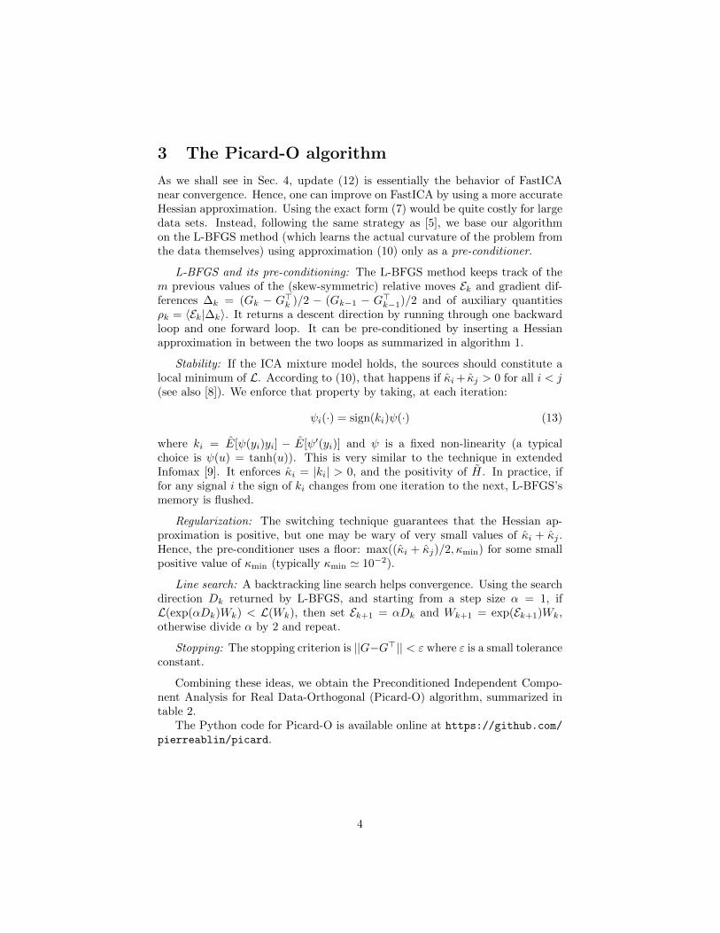
As we shall see in Sec. 4, update (12) is essentially the behavior of FastICAnear convergence. Hence, one can improve on FastICA by using a more accurateHessian approximation. Using the exact form (7) would be quite costly for largedata sets. Instead, following the same strategy as [5], we base our algorithmon the L-BFGS method (which learns the actual curvature of the problem fromthe data themselves) using approximation (10) only as a pre-conditioner.
L-BFGS and its pre-conditioning: The L-BFGS method keeps track of them previous values of the (skew-symmetric) relative moves Ek and gradient dif-ferences ∆k = (Gk − G>k )/2 − (Gk−1 − G>k−1)/2 and of auxiliary quantitiesρk = 〈Ek|∆k〉. It returns a descent direction by running through one backwardloop and one forward loop. It can be pre-conditioned by inserting a Hessianapproximation in between the two loops as summarized in algorithm 1.
Stability: If the ICA mixture model holds, the sources should constitute alocal minimum of L. According to (10), that happens if κi+ κj > 0 for all i < j(see also [8]). We enforce that property by taking, at each iteration:
ψi(·) = sign(ki)ψ(·) (13)
where ki = E[ψ(yi)yi] − E[ψ′(yi)] and ψ is a fixed non-linearity (a typicalchoice is ψ(u) = tanh(u)). This is very similar to the technique in extendedInfomax [9]. It enforces κi = |ki| > 0, and the positivity of H. In practice, iffor any signal i the sign of ki changes from one iteration to the next, L-BFGS’smemory is flushed.
Regularization: The switching technique guarantees that the Hessian ap-proximation is positive, but one may be wary of very small values of κi + κj .Hence, the pre-conditioner uses a floor: max((κi + κj)/2, κmin) for some smallpositive value of κmin (typically κmin ' 10−2).
Line search: A backtracking line search helps convergence. Using the searchdirection Dk returned by L-BFGS, and starting from a step size α = 1, ifL(exp(αDk)Wk) < L(Wk), then set Ek+1 = αDk and Wk+1 = exp(Ek+1)Wk,otherwise divide α by 2 and repeat.
Stopping: The stopping criterion is ||G−G>|| < ε where ε is a small toleranceconstant.
Combining these ideas, we obtain the Preconditioned Independent Compo-nent Analysis for Real Data-Orthogonal (Picard-O) algorithm, summarized intable 2.
The Python code for Picard-O is available online at https://github.com/pierreablin/picard.
4

Algorithm 1: Two-loop recursion L-BFGS formula
Input : Current gradient Gk, moments κi, previous El, ∆l, ρl∀l ∈ {k −m, . . . , k − 1}.
Set Q = −(Gk −G>k )/2;for l=k-1,. . . ,k-m do
Compute al = ρl〈El|Q〉 ;Set Q = Q− al∆i ;
end
Compute D as Dij = Qij/max(κi+κj
2 , κmin
);
for l=k-m,. . . ,k-1 doCompute β = ρl〈∆l|D〉 ;Set D = D + El(al − β) ;
endOutput: Descent direction D
Algorithm 2: The Picard-O algorithm
Input : Initial signals X, number of iterations KSphering: compute W0 by (1) and set Y = W0X;for k = 0 · · ·K do
Compute the signs sign(ki) ;Flush the memory if the sign of any source has changed ;Compute the gradient Gk ;Compute search direction Dk using algorithm 1 ;Compute the step size αk by line search ;Set Wk+1 = exp(αkDk)Wk and Y = Wk+1X ;Update the memory;
endOutput: Unmixed signals Y , unmixing matrix Wk
4 Link with FastICA
This section briefly examines the connections between Picard-O and symmetricFastICA [10]. In particular, we show that both methods essentially share thesame solutions and that the behavior of FastICA is similar to a quasi-Newtonmethod.
Recall that FastICA is based on an N × N matrix C(Y ) matrix definedentry-wise by:
Cij(Y ) = E[ψi(yi)yj ]− δijE[ψ′i(yi)] . (14)
The symmetric FastICA algorithm, starting from white signals Y , can be seenas iterating Y ← Cw(Y )Y until convergence, where Cw(Y ) is the orthogonalmatrix computed as
Cw(Y ) = (CC>)−12C . (15)
5
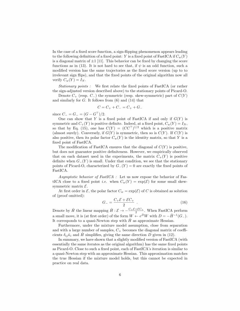
In the case of a fixed score function, a sign-flipping phenomenon appears leadingto the following definition of a fixed point: Y is a fixed point of FastICA if Cw(Y )is a diagonal matrix of ±1 [11]. This behavior can be fixed by changing the scorefunctions as in (13). It is not hard to see that, if ψ is an odd function, such amodified version has the same trajectories as the fixed score version (up to toirrelevant sign flips), and that the fixed points of the original algorithm now allverify Cw(Y ) = IN .
Stationary points : We first relate the fixed points of FastICA (or ratherthe sign-adjusted version described above) to the stationary points of Picard-O.
Denote C+ (resp. C−) the symmetric (resp. skew-symmetric) part of C(Y )and similarly for G. It follows from (6) and (14) that
C = C+ + C− = C+ +G−
since C− = G− = (G−G>)/2.One can show that Y is a fixed point of FastICA if and only if G(Y ) is
symmetric and C+(Y ) is positive definite. Indeed, at a fixed point, Cw(Y ) = IN ,so that by Eq. (15), one has C(Y ) = (CC>)1/2 which is a positive matrix(almost surely). Conversely, if G(Y ) is symmetric, then so is C(Y ). If C(Y ) isalso positive, then its polar factor Cw(Y ) is the identity matrix, so that Y is afixed point of FastICA.
The modification of FastICA ensures that the diagonal of C(Y ) is positive,but does not guarantee positive definiteness. However, we empirically observedthat on each dataset used in the experiments, the matrix C+(Y ) is positivedefinite when G−(Y ) is small. Under that condition, we see that the stationarypoints of Picard-O, characterized by G−(Y ) = 0 are exactly the fixed points ofFastICA.
Asymptotic behavior of FastICA : Let us now expose the behavior of Fas-tICA close to a fixed point i.e. when Cw(Y ) = exp(E) for some small skew-symmetric matrix E .
At first order in E , the polar factor Cw = exp(E) of C is obtained as solutionof (proof omitted):
G− =C+E + EC+
2. (16)
Denote by H the linear mapping H : E → −C+E+EC+
2 . When FastICA perform
a small move, it is (at first order) of the form W ← eDW with D = −H−1(G−).It corresponds to a quasi-Newton step with H as approximate Hessian.
Furthermore, under the mixture model assumption, close from separationand with a large number of samples, C+ becomes the diagonal matrix of coeffi-cients δij κi and H simplifies, giving the same direction D given in (12).
In summary, we have shown that a slightly modified version of FastICA (withessentially the same iterates as the original algorithm) has the same fixed pointsas Picard-O. Close to such a fixed point, each of FastICA’s iteration is similar toa quasi-Newton step with an approximate Hessian. This approximation matchesthe true Hessian if the mixture model holds, but this cannot be expected inpractice on real data.
6
5 Experiments
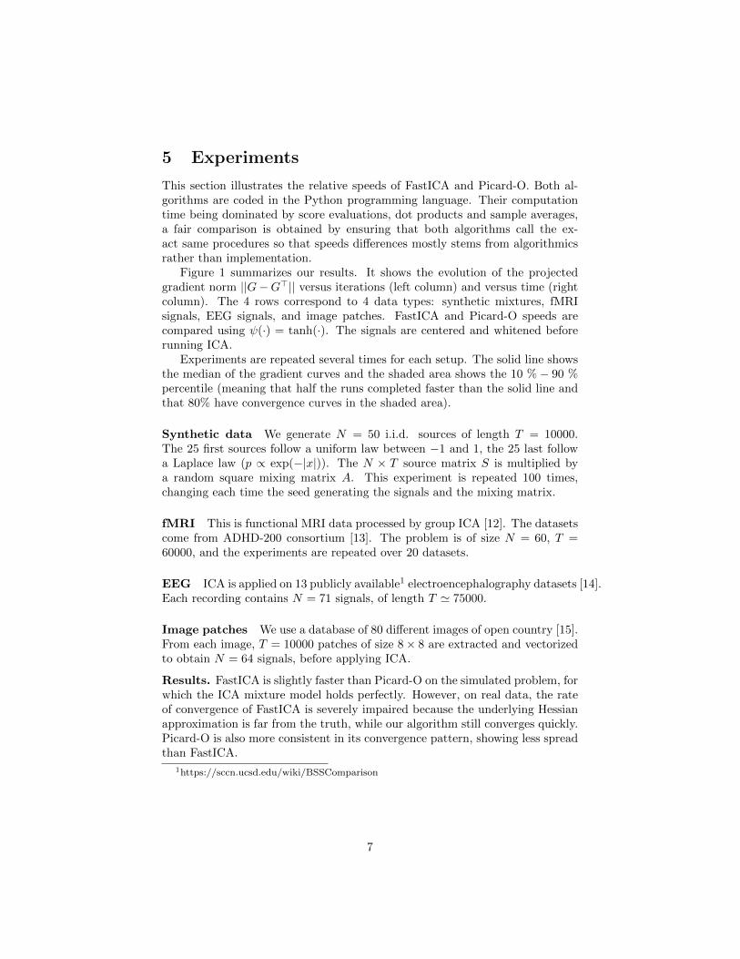
This section illustrates the relative speeds of FastICA and Picard-O. Both al-gorithms are coded in the Python programming language. Their computationtime being dominated by score evaluations, dot products and sample averages,a fair comparison is obtained by ensuring that both algorithms call the ex-act same procedures so that speeds differences mostly stems from algorithmicsrather than implementation.
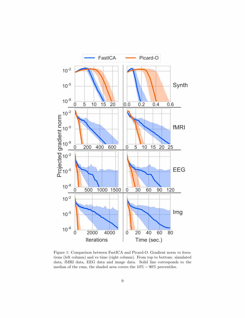
Figure 1 summarizes our results. It shows the evolution of the projectedgradient norm ||G−G>|| versus iterations (left column) and versus time (rightcolumn). The 4 rows correspond to 4 data types: synthetic mixtures, fMRIsignals, EEG signals, and image patches. FastICA and Picard-O speeds arecompared using ψ(·) = tanh(·). The signals are centered and whitened beforerunning ICA.
Experiments are repeated several times for each setup. The solid line showsthe median of the gradient curves and the shaded area shows the 10 %− 90 %percentile (meaning that half the runs completed faster than the solid line andthat 80% have convergence curves in the shaded area).
Synthetic data We generate N = 50 i.i.d. sources of length T = 10000.The 25 first sources follow a uniform law between −1 and 1, the 25 last followa Laplace law (p ∝ exp(−|x|)). The N × T source matrix S is multiplied bya random square mixing matrix A. This experiment is repeated 100 times,changing each time the seed generating the signals and the mixing matrix.
fMRI This is functional MRI data processed by group ICA [12]. The datasetscome from ADHD-200 consortium [13]. The problem is of size N = 60, T =60000, and the experiments are repeated over 20 datasets.
EEG ICA is applied on 13 publicly available1 electroencephalography datasets [14].Each recording contains N = 71 signals, of length T ' 75000.
Image patches We use a database of 80 different images of open country [15].From each image, T = 10000 patches of size 8× 8 are extracted and vectorizedto obtain N = 64 signals, before applying ICA.
Results. FastICA is slightly faster than Picard-O on the simulated problem, forwhich the ICA mixture model holds perfectly. However, on real data, the rateof convergence of FastICA is severely impaired because the underlying Hessianapproximation is far from the truth, while our algorithm still converges quickly.Picard-O is also more consistent in its convergence pattern, showing less spreadthan FastICA.
1https://sccn.ucsd.edu/wiki/BSSComparison
7
6 Discussion
In this paper, we show that, close from its fixed points, FastICA’s iterationsare similar to quasi-Newton steps for maximizing a likelihood. Furthermore,the underlying Hessian approximation matches the true Hessian of the problemif the signals are independent. However, on real datasets, the independenceassumption never perfectly holds. Consequently, FastICA may converge veryslowly on applied problems [16] or can get stuck in saddle points [17].
To overcome this issue, we propose the Picard-O algorithm. As an extensionof [5], it uses a preconditioned L-BFGS technique to solve the same minimiza-tion problem as FastICA. Extensive experiments on three types of real datademonstrate that Picard-O can be orders of magnitude faster than FastICA.
8
0 5 10 15 2010-8
10-5
10-2
0.0 0.2 0.4 0.6
0 200 400 60010-8
10-5
10-2
0 5 10 15 20 25
0 500 1000 150010-8
10-5
10-2
0 30 60 90 120
0 2000 4000Iterations
10-8
10-5
10-2
0 20 40 60 80Time (sec.)
FastICA Picard-OP
roje
cted
gra
dien
t nor
m
fMRI
Synth
Img
EEG
Figure 1: Comparison between FastICA and Picard-O. Gradient norm vs itera-tions (left column) and vs time (right column). From top to bottom: simulateddata, fMRI data, EEG data and image data. Solid line corresponds to themedian of the runs, the shaded area covers the 10%− 90% percentiles.
9
References
[1] P. Comon, “Independent component analysis, a new concept?” Signal Pro-cessing, vol. 36, no. 3, pp. 287 – 314, 1994.
[2] A. Hyvarinen, “Fast and robust fixed-point algorithms for independentcomponent analysis,” IEEE Transactions on Neural Networks, vol. 10,no. 3, pp. 626–634, 1999.
[3] E. Oja and Z. Yuan, “The fastica algorithm revisited: Convergence analy-sis,” IEEE Transactions on Neural Networks, vol. 17, no. 6, pp. 1370–1381,2006.
[4] H. Shen, M. Kleinsteuber, and K. Huper, “Local convergence analysis ofFastICA and related algorithms,” IEEE Transactions on Neural Networks,vol. 19, no. 6, pp. 1022–1032, 2008.
[5] P. Ablin, J.-F. Cardoso, and A. Gramfort, “Faster independent componentanalysis by preconditioning with hessian approximations,” Arxiv Preprint,2017.
[6] D. T. Pham and P. Garat, “Blind separation of mixture of independentsources through a quasi-maximum likelihood approach,” IEEE Transac-tions on Signal Processing, vol. 45, no. 7, pp. 1712–1725, 1997.
[7] W. Bertram, “Differential Geometry, Lie Groups and Symmetric Spacesover General Base Fields and Rings,” Memoirs of the American Mathe-matical Society, 2008.
[8] J.-F. Cardoso, “On the stability of some source separation algorithms,” inProc. of the 1998 IEEE SP workshop on neural networks for signal pro-cessing (NNSP ’98), 1998, pp. 13–22.
[9] T.-W. Lee, M. Girolami, and T. J. Sejnowski, “Independent componentanalysis using an extended infomax algorithm for mixed subgaussian andsupergaussian sources,” Neural computation, vol. 11, no. 2, pp. 417–441,1999.
[10] A. Hyvarinen, “The fixed-point algorithm and maximum likelihood esti-mation for independent component analysis,” Neural Processing Letters,vol. 10, no. 1, pp. 1–5, 1999.
[11] T. Wei, “A convergence and asymptotic analysis of the generalized sym-metric FastICA algorithm,” IEEE transactions on signal processing, vol. 63,no. 24, pp. 6445–6458, 2015.
[12] G. Varoquaux, S. Sadaghiani, P. Pinel, A. Kleinschmidt, J.-B. Poline,and B. Thirion, “A group model for stable multi-subject ICA on fMRIdatasets,” Neuroimage, vol. 51, no. 1, pp. 288–299, 2010.
10
[13] A.-. Consortium, “The ADHD-200 consortium: a model to advance thetranslational potential of neuroimaging in clinical neuroscience,” Frontiersin systems neuroscience, vol. 6, 2012.
[14] A. Delorme, J. Palmer, J. Onton, R. Oostenveld, and S. Makeig, “Indepen-dent EEG sources are dipolar,” PloS one, vol. 7, no. 2, p. e30135, 2012.
[15] A. Oliva and A. Torralba, “Modeling the shape of the scene: A holisticrepresentation of the spatial envelope,” International journal of computervision, vol. 42, no. 3, pp. 145–175, 2001.
[16] P. Chevalier, L. Albera, P. Comon, and A. Ferreol, “Comparative perfor-mance analysis of eight blind source separation methods on radiocommuni-cations signals,” in Proc. of IEEE International Joint Conference on NeuralNetworks, vol. 1, 2004, pp. 273–278.
[17] P. Tichavsky, Z. Koldovsky, and E. Oja, “Performance analysis of the Fas-tICA algorithm and cramer-rao bounds for linear independent componentanalysis,” IEEE transactions on Signal Processing, vol. 54, no. 4, pp. 1189–1203, 2006.
11