FASTENING ANALYSIS USING LOW FIDELITY FINITE ELEMENT …

FASTENING ANALYSIS USING LOW FIDELITY FINITEELEMENT MODELS

Rodrigo de Sá Martins∗ , Marco Túlio dos Santos∗∗, Ernani Sales Palma∗∗Universidade Federal de Minas Gerais , ∗∗Embraer

Keywords: Joints, finite elements, fastener stiffness, joint load distribution

Abstract

There are several ways to create a finite elementmodel of a fastener. The models are divided intotwo categories: low-fidelity models and high-fidelity models. The former is usually used in thesub-component analysis and the latter when deal-ing with details. Low-fidelity models are simplermodels, using a static linear solution and one-dimensional elements for the fasteners. The pur-pose of this type of model is to obtain a loaddistribution in a joint. High-fidelity models usesolutions with displacement and material nonlin-earities, as well as contact, friction, etc. They areused when it is desired to verify the influence ofdifferent effects on the resistance of the joint (theinterference, the friction, the size of the head ofthe fastener, etc.). High fidelity models are notalways more accurate when compared to low fi-delity models. This is because the non-linearitiesintroduced in the model to simulate the associ-ated physical phenomena may include undesir-able numerical errors. To use high fidelity mod-els, strict validation is required. The paper re-views the methods that are currently used to ana-lyze fasteners using finite element analysis.

1 Introduction

An aircraft structure is assembled from manycomponents. These components can be madefrom thin skins and extrusions, as well as ma-chined, cast and forged parts. When connected,these components form the major sub-assembliesof the airplane. Ideally, each component should

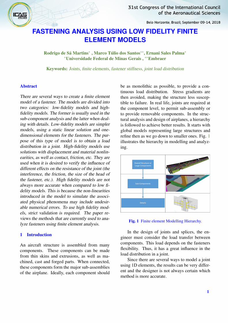
be as monolithic as possible, to provide a con-tinuous load distribution. Stress gradients arethen avoided, making the structure less suscep-tible to failure. In real life, joints are required atthe component level, to permit sub-assembly orto provide removable components. In the struc-tural analysis and design of airplanes, a hierarchyis followed to achieve better results. It starts withglobal models representing large structures andrefine then as we go down to smaller ones. Fig. 1illustrates the hierarchy in modelling and analyz-ing.

Fig. 1 Finite element Modelling Hierarchy.

In the design of joints and splices, the en-gineer must consider the load transfer betweencomponents. This load depends on the fastenersflexibility. Thus, it has a great influence in theload distribution in a joint.

Since there are several ways to model a jointusing 1D elements, the results can be very differ-ent and the designer is not always certain whichmethod is more accurate.

1

RODRIGO DE SÁ MARTINS , MARCO TÚLIO DOS SANTOS , ERNANI SALES PALMA

1.1 Axial Stiffness

To define the axial stiffness of mechanically fas-tened joints with no pre-torque (such as rivetedjoints), can be approximated by a single rod[1].The standard formula for a single rod is definedin equation 1.

k =E f A

t1 + t2=

E f

(πd2

4

)t1 + t2

(1)

1.2 Transverse Stiffness

There are extra difficulties to obtain a generalanalytic formula to estimate transverse stiffness.Several empirical studies had been made and thefinal results of some of them are presented here.For more information refer to [1], [2], [3],[4], and[5].

• Swiftf =

5E f d

+0.8t1E1

+0.8t2E2

(2)

• Grumman

f =(t1 + t2)2

E f d3 +3.7( 1

t1E1+

1t2E2

)(3)

• Huth

f =(t1 + t2

2d

)bn

( 1E1t1

+1

nE2t2

+1

nE f t1+

12nE f t2

) (4)

• Tate and Rosenfeld

f =1

E f t1+

1E f t2

+1

E1t1+

+32

9E f πd2 (1+ν f )(t1 + t2)+

+8

5E f πd4 +(

t31 ++5t2

1 t2+

+5t1t22 + t3

2

)(5)

• Morris

f ={(2845

EL1t1+

2845EL2t2

)+ c f

[( 500E f t1

+

1000EST1t1

)(t1d

)2+( 500

E f t2+

1000EST2t2

)×(t2

d

)2(dhead

d

)−0.34( sd

)−0.5( pd

)0.34e0.3r

(6)

When the mesh is refined enough, a hole canbe modeled with at least eight nodes[4]. Whendealing with a coarser mesh, the union can bemade by nodes or elements. Fig. 2 and Fig. 3shows fasteners modelled as element do elementand node to node conections respectively.

Fig. 2 Detailed Model an elevator[4].

Fig. 3 Detailed Model of a leading edge[4].

1.3 Multi Spring Models

The "multi-spring" modelling method, createdby Rutman [6], is one of the most used in theaerospace industry and presents several advan-tages when compared with others. The most sig-nificant advantage comes from the fact that it canbe used for any joint, with any number of ele-ments joined together. Rutman’s modelling tech-nique differs from the traditional approach of alap joint with a unique link element.

2

FASTENING ANALYSIS USING LOW FIDELITY FINITE ELEMENT MODELS

The traditional approach cannot be used forother joint configurations or joints with a largernumber of connected components. The Rut-man procedure is free from these limitations.However, Rutman did not validate his findingsthrough experiments.

In the Rutman modelling technique describedusing the NASTRAN software, the fastener isrepresented by a CBAR (Beam) element and thecontact between the plates and the fasteners isrepresented by a CBUSH (Spring) element.

The following components of rigidity areconsidered:

• Translational stiffness on plate bearing;

• Translational stiffness of the fastener bear-ing;

• Rotational stiffness on plate bearing;

• Rotational stiffness of the fastener bearing;

• Shear stiffness of the fastener;

• Bending stiffness of the fastener.

Fig. 4 illustrate the elements used in themulti-spring modelling approach.

Fig. 4 Multi Spring Model [6].

For more information please refer to refer-ence [7] and [6].

2 Modelling Comparison Techniques

2.1 Flexibility equation comparison

For the following section, a series of models werebuilt and the fastener stiffness(an input for the 1Delement) was compared with the expected value.Since the sheet flexibility is known, the fastenerflexibility can be indirectly estimated by[1]:

f =(

δtotal

Ftotal−

l0 + 12 l1 + l2EA

)(7)

In this step, the models will be made in NAS-TRAN using different modelling techniques. Thecomparison will be carried out in the followingway: The joint will be modeled, and it will beassigned a stiffness value according to the corre-sponding equation. The error of the modellingtechnique is computed as the difference betweenthe expected stiffness (assigned to the spring us-ing the empirical equation), and the measuredjoint stiffness using equation 7.

The test data used in this paper can be foundin [1]. Since Morris equation was developed tofit in the data he collected, the comparison of dif-ferent approaches will be made using his expres-sion.

The mesh will be composed of square ele-ments 2mm wide. The load was 0.4mm of en-forced displacement. The models will be dividedinto four categories and for each of them, onemodel will be generated with the rigidity relativeto each empirical equation. The categories are:

1 - Model with gap: Models with the platesmodeled on the middle surface with a gapthat is the result of the distance between thecenter lines of the plates, that is, equal tothe sum of the thicknesses over two. Themodel used is shown in Fig. 5.

3


Fig. 5 Model with gap between shell elements

2 - Gap with Rigid Element Model: Modelswith the plates modeled on the middlesurface, exactly as before, however usingthe rigid element technique shown in Fig.6.

A rigid element is created by replacing thelink. It connects one of the plates to an aux-iliary node created that matches the nodeon the next plate. The spring is then cre-ated between the two matching nodes.

Visually the model is exactly as in Fig. 5,but conceptually, it is eliminated (at least intheory) the secondary bending.

Fig. 6 Technique of rigid element to model fas-teners [8].

3 - No gap model: Models with the plates mod-eled in the plane of the connection, with thebinding elements with infinitesimal length.See Fig. 7.

Fig. 7 Model with no offset between shell elements

4 - Element offset model: Models with theplates modeled in the plane of the con-nection, with the offset applied to theshell element, maintaining the bendingstiffness of the assembly. The technique isillustrated in Fig. 8.

Fig. 8 Model with no offset between shell ele-ments and internal offset in the element property

Table 1 Comparison between modelling techniquesModel Fx (daN) f (mm/daN) k (daN/mm)

kexpected(daN/mm) Difference

1 192.3 0.00231111 432.69 1215 64%2 153.1 0.00337505 296.29 76%3 283.0 0.00097805 1022.44 16%4 254.1 0.00129978 769.36 37%

From the results obtained, shown in table 1,it can be seen that the numerical results are verypoor. Even when the elimination of the sourcesof error, such as plates modeled in the same plane(type 3 modelling), the results still show signifi-cant differences.

When evaluating the results of the other mod-els, it is noticed that the connection has becomeso flexible that it represents very little the actualstructure. The following list will present somepossible reasons for why this discrepancy mayhave occurred and then each hypothesis will benumerically evaluated.

4


1) The model can be very refined so that eachelement no longer meets the plate condi-tion (two dimensions much larger than theother). According to [9], the ratio shouldbe at least 1/20. This is hardly observed inrefined models (for example, the thicknessis equal to 1.27mm and the element sizeequal to 2mm). It is clear that the authorrefers in the overall analysis (dimensions ofthe specimen and not of the elements), butsince there is a concentrated load, it maybe that the model does not work well in theelements close to the connection, causing alarge decrease in local rigidity.

Thus, it is suggested the evaluation of the re-lationship between mesh size and the calculatedstiffness.

2) The next test would be to model the holeand create a rigid element to join the partsthrough a connector.

2.2 Study of the mesh size

In order to better understand the first hypothesisthat pointed out for the differences between thestiffness that is used in the spring element in themodel and the stiffness calculated through equa-tion 7 , the calculation was redone by varying thesize of the mesh. In this case, it was used as inputthe rigidity calculated with the Grumman equa-tion and the plates modeled in the same plane(condition where the smallest error was found inthe previous item). The result is shown in Fig. 9.

Mesh size(mm)0 2 4 6 8 10 12 14 16

Err

or

-21.2%

-17.8%

-15.0%

-12.5%

-5.4%

-21.2%

-17.8%

-15.0%

-12.5%

-5.4%

Fig. 9 Influence of mesh size in the joint stiffnesserror.

As it was expected, the error tends to decreasewhen the mesh size increases. However, makinga mesh as coarse as possible alone does not solvethe problem of modelling fasteners, once, in gen-eral, the engineer needs to use models refinedenough to represent the geometry. The modelof the joint is simple enough to allow the useof elements 16mm wide. Even with the meshthis coarse mesh (Fig. 10), the error was not ne-glectable.

Fig. 10 Joint model with element size equal to16mm.

2.3 Study of additional modelling techniques

More ways of modelling are tested below. Theyare compared to the base model, with an elementsize equal to 2 millimeters. The base model willbe denoted by "Model 1". The next configura-tion would be to create a RBE3[7] interpolationelement in the area of influence of the fastener,i.e., all nodes that are at a distance of half the di-ameter. This model, shown in Fig. 11, will bedenoted by "Model 2".

Fig. 11 Model 2 details.

5


Next, a model with the same mesh size wasbuilt, but the hole was modeled as shown in Fig.12. This model will be denoted by "Model 3".

Fig. 12 Model 3 details.

The three models were built with gap (platesmodeled in the original center line) and withoutoffset (plates modeled in the same plane). Theresults are shown in table 2.

Table 2 Results of the improved models.Condition Model Force f k k Error

(daN) (mm/daN) (daN/mm) expected(daN/mm)

With gap 1 191.2 0.00233468 428.32 1214.66 -65%2 209.9 0.00196258 509.53 -58%3 205.6 0.00204217 489.68 -60%

Without gap 1 280.7 0.00100162 998.38 -18%2 295.6 0.00085704 1166.81 -4%3 292.1 0.00088966 1124.03 -7%

It can be seen that the improvements are quiteeffective, especially when the error associatedwith the gap condition is removed. Model 2 gota relatively low error, even with a refined mesh.

3 Comparison with experimental results

In this section the experimental results shownin [1] are compared with finite element models.Models were created (one for each modelling ap-proach) containing the four test specimens whoseresults are shown in section 3.2. One of the mod-els is shown in Fig. 13.

Fig. 13 Finite Element Models for validationwith test specimens.

It was noticed that the model of simple springthat obtained less numerical error was the modelwith the plates are modeled in the same plane anda rigid element is modeled in the nodes in the areaof influence of the fastener. The Multi-Springsmodel will be used with the same characteristics,except that the plates will be modeled on theiroriginal average surfaces. To have a fair compar-ison, the simple spring model will be modeledalso on the original surface.

Fig. 14 shows the comparison for the 1 rowspecimen.

Displacement(mm)

0 0.05 0.1 0.15 0.2 0.25 0.3 0.35 0.4

Reaction Force(daN)

0

50

100

150

200

250Model comparison of a joint with 1 row

Test DataRutman ModelMorris Model with gapMorris Model without gap

Fig. 14 Comparison between numerical and ex-perimental data for the 1 row specimen.

It can be seen that the best results for this casewere for the model using Morris stiffness withoutgap. The Rutman and Morris models without gapobtained very similar poor results. This can beexplained by the excessive secondary bending ofthe model that rotate the connection causing themodel to move more than the specimen.

For models with two rows of rivets, the re-sults were compared with the three test specimen

6


results provided in [1]. The comparison is shownin Fig. 15.

Displacement(mm)

0 0.05 0.1 0.15 0.2 0.25 0.3 0.35 0.4 0.45 0.5

Reaction Force(daN)

0

50

100

150

200

250

300

350

400Model comparison of a joint with 2 rows

Data from test 1Data from test 2Data from test 3Rutman ModelMorris Model with gapMorris Model without gap

Fig. 15 Comparison between numerical and ex-perimental data for the 2 rows specimen.

Again, the Morris model with no gap is closerto that obtained in the tests, followed by the Rut-man Model and the Morris model with gap. Fig.16 shows the result for the three-row rivet model.

Displacement(mm)

0 0.1 0.2 0.3 0.4 0.5 0.6 0.7 0.8

Reaction Force(daN)

0

100

200

300

400

500

600




In this case, the results were closer, and, theRutman model behaved slightly better than theMorris model without gap. The Morris modelwith gap continued with more flexible resultsthan the test. Next, in Fig. 17, the results areshown for four-row rivet models.

Displacement(mm)

0 0.1 0.2 0.3 0.4 0.5 0.6 0.7 0.8

Reaction Force(daN)

0

100

200

300

400

500

600

700

800




In this case, all the results are reasonablygood. The best approximation was the Morrismodel without gap.

Comparison with the tests gives a new per-spective on the accuracy of the models. In gen-eral, the model using the Morris equation andwithout modelling the gap has the best result. Asthe number of rivets increases, the Rutman modeltends to become stiffer and therefore closer to thetest. In the four-row test, Rutman’s model getsstiffer than the test and that can be an issue. Thisputs in check the trend of greater precision in afive-row test, for example.

Another point to consider is the fact that theMorris equation was empirically developed withthe same data that was used. Therefore, all pa-rameters were obtained by minimizing the er-ror with the test, something that was not donewith the Rutman model. Even so, when mod-elling gap structures (something extremely rec-ommended for large assemblies), the error intro-duced by the model will significantly worsen theresult.

Finally, it should be remembered that thestudy was performed for lap joints. In an aero-nautical structure, there are several other types ofriveted joints, such as butt joints, double shearand tension.

7


4 Use of high-fidelity models to compare themodelling techniques

Finally, to have a better understanding of the be-havior and the accuracy of each modelling tech-nique in other types of models, a high-fidelitymodel is built and its result is assumed to be cor-rect. In order to make that assumption, the non-linear model parameters will be calibrated withthe four specimen tested by Morris[1]. With themodels calibrated, the same parameters will beused for all the other models.

4.1 Calibration of the high-fidelity models

The models were built in Altair Hypermesh [10]and the solver that was used were RADIOSS[11].The baseline model were the one with two rowsof fasteners. This choice was obvious, since it isthe configuration which has the most data.

The model has 64898 nodes and 51814 el-ements. The elements are mostly eight-nodebricks. The gap between the elements is 0.15mmand the friction coefficient is 0.3.

The test procedure was developed by Huth[2]. He tested several specimens with 6000 Fal-staff loading cycles. The flexibility results afterthe cycles were the same of a quasi-static load-ing test at two thirds of the maximum load. Thefinite element analysis is non-linear static with alinear enforced displacement in one end of theplate. The curve was draw based in the Ramberg-Osgood 3 parameters)[12]. The material data wasfound in [13]. To comply with the test a penaltyfactor was applied equals to 2/3. The results forthe 1 row specimen is shown in Fig. 18.

Displacement(mm)

0 0.05 0.1 0.15 0.2 0.25 0.3 0.35 0.4

Reaction Force(daN)

0

50

100

150

200

250Model validation of the joint with 1 row

Test Data

FEM

Fig. 18 High-fidelity model results of the onerow specimen.

The model accuracy was observed in themodels with two, three and four row of fasten-ers too.This proves that the penalty factor of 2/3is shown to be effective. Thus, the high-fidelitymodels can be then used to calibrate the low-fidelity ones. The next step consists in comparingthe 1D approaches best (single and multi-spring)to model different joint configuration using thedetailed model as a baseline.

4.2 Double Shear Joints

In this section the approaches of Rutman andMorris are compared with the detailed models us-ing a single line of one to four fasteners. Bothmodels use gap between plates. The results areshown in Fig. 19.

Displacement(mm)

0 0.05 0.1 0.15 0.2 0.25 0.3 0.35 0.4 0.45

Reaction Force(daN)

0

50

100

150

200

250

300

350Double Shear 1 fastener

Rutman

Morris

Detailed Model

Fig. 19 Comparison between 1D and 3D fasten-ers modelling of a 1 row double shear joint.

As can be seen from 19, the Rutman modelis very close to the detailed one. The small dif-

8


ference occurs only in the nonlinear part of theDetailed Model.

Displacement(mm)

0 0.05 0.1 0.15 0.2 0.25 0.3 0.35 0.4 0.45

Reaction Force(daN)

0

50

100

150

200

250

300

350

400

450

500Double Shear 2 fasteners

Rutman

Morris

Detailed Model

Fig. 20 Comparison between 1D and 3D fasten-ers modelling of a 2 rows double shear joint.

Fig. 20 shows that both approaches tend tomake the fastening more rigid when compared tothe detailed model.

Using free-body diagrams it is possible to de-termine the load on each row of fasteners. Theload on each fastener was obtained using thestresses before and after the fasteners. Fig. 21shows the procedure to obtain the fastener loadin the detailed model.

Fig. 21 Free body diagram of a joint model.

Fig. 22 shows the obtained results.

Rows

1 1.1 1.2 1.3 1.4 1.5 1.6 1.7 1.8 1.9 2

Load Distribution

30%

35%

40%

45%

50%

55%

60%

65%

70%Double Shear 2 fasteners

Rutman

Morris

Detailed Model

Fig. 22 Load distribution in 2 rows double shearjoint.

Although the average stiffness of the 1D jointmodels are higher that the detailed model, theload on the fasteners are non-conservative whencompared to the detailed model (the detailedmodel presents a higher load concentration).

The tendency of the models to get stiffer andnon-conservative increases with the number offasteners in the joint. The difference betweenload distributions of single spring and multi-spring models are neglectable when compared tothe detailed models.

4.3 Butt Joints

This section continue the study performed before.The main objective is to assert if the tendenciescontinue be observed for butt joints. Fig. 23shows the results for the butt joint with one row.

Displacement(mm)

0 0.05 0.1 0.15 0.2 0.25 0.3 0.35 0.4 0.45

Reaction Force(daN)

0

20

40

60

80

100

120

140

160

180Butt Joint 1 fastener

Rutman

Morris

Detailed Model

Fig. 23 Comparison between 1D and 3D fasten-ers modelling of a 1 row butt joint.

The detailed model is much more rigid thanthe 1D models. The Rutman model provide a bet-ter representation, but still a poor representationof the joint behavior.

It was noticed that by using the same param-eter as in the calibration, the detailed models ofthe 3x3 and 4x4 butt joint took several hours torun and presented a very unusual behavior. Thus,only the results from the 1x1 and 2x2 lap jointswill be analyzed. In the case of a butt joint, thedetailed model tends to be stiffer than the linearones. On the other hand, the load distribution ofthe linear models tends to be conservative whencompared to the detailed ones.

9


5 Conclusions

Based on the analyzes and results obtained, thefollowing conclusions can be drawn:

• The results of the numerical experimentswith the low-fidelity models show that themajor sources of error in the modelling offasteners is the secondary bending gener-ated by the gap between the plates.

• Another source of error in fastener modelsis discrete load transfer. It has been ob-served that an efficient way of reducing er-ror is by dividing the load in the area ofinfluence of the fastener, being effective inall forms of modelling (single spring andmulti-springs).

• The multi-spring model has been shownto be less sensitive to excessive secondarybending, however, as the number of rivetsincreases, it begins to become stiffer thanthe tested values.

• For the case of double and butt shear joints,none of the models presented satisfactoryresults. This shows that specific tests forthese configurations are necessary for thedevelopment of more robust methodolo-gies.

References

[1] Geoff Morris. Defining a standard formula andtest-method for fastener flexibility in lap-joints.PhD thesis, Technical University Delft, 2004.

[2] Heimo Huth. Influence of fastener flexibility onthe prediction of load transfer and fatigue lifefor multiple-row joints. In ASTM, editor, Fa-tigue in Mechanically Fastened Composite andMetallic Joints, page 30, 1985.

[3] S. Rosenfeld M. B. Tate. Preliminary investiga-tion on loads carried by individual joints - naca-tn-1051. Technical report, 1946.

[4] Rodrigo Martins. Investigação da precisão demodelos de juntas rebitadas utilizando elemen-tos finitos, 2018.

[5] Swift T. Development of fail-safe design fea-tures of the dc-10. damage tolerance in aircraftstructures. Technical report, 1971.

[6] Alexander Rutman. Fasteners modeling formsc.nastran finite element analysis. In SAE In-ternationa, editor, World Aviation Conference.,page 19, 2000.

[7] MD/MSC. Md/msc nastran quick referenceguide. Technical report, MSC.Software Corpo-ration., 2010.

[8] Rodrigo Martins. Influence of types of dis-crete modelling of fasteners in fem models.In NAFEMS, editor, NAFEMS World Congress2017, page 26, 2017.

[9] A. Ugural. Stresses In Plates and Shells.McGraw-Hill, 1st edition edition, 1991.

[10] Altair. Hypermesh introduction pre-processingmodels for finite element analysis. Technical re-port, 2016.

[11] Altair. Radios user guide. Technical report,2017.

[12] William R. Osgood Walter Ramberg. Descrip-tion of stress-strain curves by three parameters.Technical report, 1943.

[13] FAA. Metallic materials properties develop-ment and standardization. Technical report,2013.

6 Contact Author Email Address

For contacting the authors, please refer to:[email protected]@[email protected]

Copyright Statement

The authors confirm that they, and/or their companyor organization, hold copyright on all of the origi-nal material included in this paper. The authors alsoconfirm that they have obtained permission, from thecopyright holder of any third party material includedin this paper, to publish it as part of their paper. Theauthors confirm that they give permission, or have ob-tained permission from the copyright holder of thispaper, for the publication and distribution of this pa-per as part of the ICAS proceedings or as individualoff-prints from the proceedings.

10

Documents

FASTENING ANALYSIS USING LOW FIDELITY FINITE ELEMENT …