FastCourse Microsoft Excel 2019 & 365 · DEVELOP YOUR SKILLS: E3-D1. In this exercise, you will create a formula using the SUM function to calculate the final grade for each . student

In this chapter, you will begin using functions in your formulas to make complex calculations quicker and easier.

You will also learn about the difference between a relative and an absolute reference and practice using both in your formulas.

L E A R N I N G O B J E C T I V E S■■ Create formulas with functions

■■ Use AutoSum

■■ Use relative and absolute cell references in formulas

■■ Define names for cells and ranges

■■ Use names in formulas

C H A P T E R T I M I N G■■ Concepts/Develop Your Skills: 1 hr 45 mins

■■ Self-Assessment: 20 mins

■■ Apply Your Skills: 40 mins

■■ Total: 2 hrs 45 mins

P R O J E C T: T R A C K I N G P R O G R E S SAs an instructor at LearnFast College, you have already recorded the student grades for your Introduction to Business course. Now you will use functions to perform a variety of calculations that will help you analyze the students’ performance.

3Performing Calculations Using Functions

E X C E L

FC19-EX-Level1.indb 67 11/3/19 3:41 PM

FastCourse Microsoft Excel 2019 & 365 © 2020 Labyrinth Learning – Not for Sale or Classroom Use

Labyrinth Learning http://www.lablearning.com

EVALUATIO

N ONLY

68 FastCourse Excel, Chapter 3: Performing Calculations Using Functions

Using Functions in FormulasFunctions are an important part of Excel. They allow you to do much more than simple mathematical operations. For example, adding two or three cells together is not a problem; however, if you needed to add up hundreds or even thousands of cells, it would be quite the tedious task! You would need a formula such as: =A1+A2+A3+A4… and so on.

The SUM function, in this case, is easier because it allows you to specify a range instead of individual cells. The function then tells Excel what operation to perform on the range, in this case addition. This is one of the reasons Excel is much more efficient than using a calculator!

Formulas with functions are inserted into a cell starting with the equals (=) sign, just like other formulas. This is followed by the function name and one or more arguments inside parentheses. An argument is the name for the numbers, cells, or ranges used in the function.

The function name SUM follows the = sign.

The function arguments must be placed inside parentheses. The argument is the range A1:A12, so Excel will add all of the values contained in that range.

This function has three arguments; two individual cells, A1 and A4, as well as the range A7:A12, separated by commas.

Functions can be typed directly into a cell, if you know the name of the function you wish to use, or inserted a number of other ways. Functions are available from the Formulas tab on the Ribbon, by using AutoSum, or by using the Insert Function button on the Formula Bar. The most common functions can be inserted quickly and easily from the AutoSum drop-down menu on the Home tab of the Ribbon.

When you insert a function by typing, Excel will suggest names for functions as you type. For example, typing =s will generate a list of functions that start with the letter S; you can ignore the prompt and type the full function name or double-click one of the suggestions that appears.




EVALUATIO

N ONLY

Using Functions in Formulas 69

DEVELOP YOUR SKILLS: E3-D1

In this exercise, you will create a formula using the SUM function to calculate the final grade for each student.

1. Start Excel; open E3-D1-SummerGrades from your Excel Chapter 3 folder and save it as: E3-D1-FallGrades

2. On the Final Grades worksheet select cell G6, and then type =SUM(C6:F6) and click Enter .

The formula in the Formula Bar shows the SUM function, and the total of cells C6:F6 is displayed in cell G6. The final grade for the first student, Ashley, is 37%.

Currently there are only two grades being added (28% and 9%). The other grades will be added to the total once they are calculated on the Quizzes and Exam worksheets.

3. In cell G7, type =SUM( and use the mouse to select the range C7:F7; then click Enter .

It’s good practice to type the closing parenthesis after the function arguments, but notice in the Formula Bar that Excel automatically inserts it for you. The sum for the second student, Atif, now shows 36%.

4. Point to the fill handle in cell G7 and double-click to fill the formula down column G.

5. Save the workbook.

The AutoSum FeatureThe AutoSum feature not only makes it easy to find some of the simplest functions, it also helps identify and enter the range of cells you are most likely to use in your function. Often when you have a column of numbers, you want to add a total at the bottom of the column. In a row, the total would be placed on the right side of the row.

AutoSum will automatically search for adjacent data, either directly above or to the left of the selected cell. Therefore, selecting the cell at the bottom of a column or the right side of a row and clicking AutoSum will very quickly enter the SUM function, as well as the range of cells necessary to add all the numbers in that column or row. If necessary, you can alter the range Excel selects by dragging to select the desired cells before completing the entry.

Another option is to select the data in the row or column first and then click AutoSum.

SUM, AVERAGE, COUNT, MAX, and MINThe SUM function is just one of the AutoSum options; other frequently used functions can be found via the AutoSum drop-down menu. These functions take a set of numbers identified in the arguments and can be used to find the average, count how many numbers are in the set, or locate the highest or lowest value. Similar to AutoSum, these functions automatically search for adjacent data, either directly above or to the left of the selected cell.




EVALUATIO

N ONLY


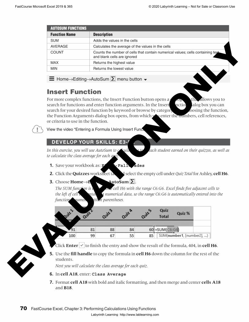
AUTOSUM FUNCTIONSFunction Name DescriptionSUM Adds the values in the cells

AVERAGE Calculates the average of the values in the cells

COUNT Counts the number of cells that contain numerical values; cells containing text and blank cells are ignored

MAX Returns the highest value

MIN Returns the lowest value

ÍÍ Home→Editing→AutoSum menu button �

Insert FunctionFor more complex functions, the Insert Function button opens a dialog box that allows you to search for functions and enter function arguments. In the Insert Function dialog box you can search for your desired function by keyword or browse by category. After choosing the function, the Function Arguments dialog box opens, from which you enter the numbers, cell references, or criteria to use in the function.

View the video “Entering a Formula Using Insert Function.”


In this exercise, you will use AutoSum to calculate the total each student earned on their quizzes, as well as to calculate the class average for each quiz.

1. S ave your workbook as: E3-D2-FallGrades

2. Click the Quizzes worksheet tab and select the empty cell under Quiz Total for Ashley, cell H6.

3. Choose Home→Editing→AutoSum .

The SUM function is entered into cell H6 with the range C6:G6. Excel finds five adjacent cells to the left of cell H6 containing numerical data, so the range C6:G6 is automatically entered into the function arguments within parentheses.

4. Click Enter to finish the entry and show the result of the formula, 404, in cell H6.

5. Use the fill handle to copy the formula in cell H6 down the column for the rest of the students.

Next you will calculate the class average for each quiz.

6. In cell A18, enter: Class Average

7. Format cell A18 with bold and italic formatting, and then merge and center cells A18 and B18.




EVALUATIO

N ONLY

Using Relative and Absolute Cell References 71

8. Select cell C18 and choose Home→Editing→AutoSum menu button �→Average.

9. Complete the entry in cell C18 and then use the fill handle to copy the average formula from cell C18 to the right, into the range D18:G18 below all five quizzes.

10. Decrease the decimal in the range of selected cells so only one decimal place is displayed and then apply bold formatting and a top cell border.

Now you want to find the average for each student.

11. Insert a new column to the left of column I.

12. Enter Student Average into cell I4.

13. Select cell I6 and choose Home→Editing→AutoSum menu button �→Average but do not complete the entry.

This time AutoSum selects the range C6:H6, which is incorrect because the average for the five quizzes should not include the total. Now you will select the correct range.

14. Use the mouse to drag and select the correct range C6:G6 and then complete the entry.

15. Use the fill handle in cell I6 to copy the formula down the column for the rest of the students.

Next you need to calculate the exam grades for each student.

16. Click the Exam worksheet tab and select the empty cell under Exam Total for Ashley, cell H6.

17. Use AutoSum to add the Section 1 to Section 5 exam marks for Ashley, and then copy the formula down column H for the other students.

18. Save your work.

Using Relative and Absolute Cell References

Cell references make it easier to copy formulas when you want to perform the same calculation with new numbers each time. Without cell references, each calculation would need to be typed individually, like with a calculator—slowly and tediously. A relative cell reference, which is the default in Excel, is one in which the location of the cell remains relative to the cell that contains the formula. This makes repeating the same calculation many times quick and easy!

For example, if the formula =A3-B3 is in cell C3, the relative position of A3 is two cells to the left of C3, and B3 is one cell to the left of C3. When you copy the formula to another cell, the cell references change to be in the same relative position. So, if you copy the formula =A3-B3 from cell C3 down to cell C4, the formula there will be =A4-B4. Excel updates the new cell references to be in the same relative position to cell C4; that is, two cells to the left and one cell to the left.

TIP! Remember that a relative cell reference changes when it is copied.




EVALUATIO

N ONLY


The copied formula is displayed with the new cell references A4 and B4.

Absolute Cell ReferencesIn some situations, you do not want the cell reference to change when you move or copy the formula. To ensure the cell reference does not change, use an absolute cell reference. You can think of an absolute cell reference as being locked in place; that is, the cell reference will not change when copied to other cells.

To make a cell reference absolute, start with a relative cell reference such as A1 and add a dollar sign in front of the column and row components, like this: $A$1.

There are two ways to create an absolute cell reference:

1. Type the cell reference and include dollar signs in front of the column and row references.

2. Use the mouse pointer to select the cell and then tap [F4] on the keyboard, which inserts both dollar signs into the cell reference at once.

Example: If the formula =$A$3-B3 is entered in cell C3 and then copied to cell C4, the formula in cell C4 would be =$A$3-B4. $A$3 is an absolute reference, so it does not change; B3 is a relative reference, so it changes to B4.

After the formula is copied, the absolute reference $A$3 does not change.

View the Video “Relative and Absolute Cell References.”

Mixed Cell ReferencesIt’s also possible to create a mix between a relative and an absolute reference in a cell reference. For example, $A3 is a reference to cell A3 where the column reference is absolute (column A will not change when copied) and the row reference is relative (row 3 will change when copied). This can be useful when copying a formula both across a row and down a column.

After you have tapped the [F4] key once, tapping it a second time changes the absolute reference to a mixed reference with only a dollar $ sign in front of the row reference. A third tap of [F4] places the dollar $ sign in front of only the column reference, and a fourth tap removes all dollar $ signs so it is once again a relative cell reference.

The original formula is seen in the Formula Bar, with relative references to both cells A3 and B3.

The original formula shows in the Formula Bar and contains an absolute reference to cell $A$3.




EVALUATIO

N ONLY

Using Relative and Absolute Cell References 73

Display and Print FormulasTo see a formula you have entered, you must first select the cell and then check the Formula Bar because it is the result of the formula that is displayed in the worksheet cell. This means that to check your formulas, you have to click each cell and review them one at a time. When you have many cells with formulas, this is very hard and time-consuming to do.

An easier way is to display all formulas within their cells. The Show Formulas button is a toggle that can be turned on and off as necessary.

TIP! You can still edit the formulas and print the worksheet while Show Formulas is turned on.

When Show Formulas is turned on, Excel automatically widens columns to show more of the cell contents.

Normally the cell must be selected for you to see the formula.

After turning on Show Formulas, the formulas display in the worksheet without selecting the cell (but you can’t see the results).

ÍÍ Formulas→Formula Auditing→Show Formulas


In this exercise, you will use formulas with absolute references to find the percentage grades for the class’s exams and quizzes.

1. Save your workbook as: E3-D3-FallGrades

2. On the Exam worksheet, enter 150 in cell H5 and 40% in cell I5.

To get a grade out of 40% for each student, you need to divide their exam score by 150 then multiply by 40%. You will use the values in cells H5 and I5 to do this.




EVALUATIO

N ONLY


3. In cell I6, type =H6/H5 but do not complete the entry.

Cell H6 shows Ashley’s total exam grade. This will change for each student when we copy the formula. Cell H5 is the number of total points the exam is worth, in this case 150, which should not change for each student; therefore, cell H5 needs to be an absolute reference.

While using [F4] to edit a formula as we will, the insertion point must be immediately before or after the reference to cell H5 or the correct cell reference won’t be converted.

4. While still in edit mode in cell I6, tap [F4] on the keyboard to make the reference for cell H5 absolute (dollar $ signs are placed in front of the column and row).

NOTE! On some keyboards, including most laptops, you must press [Fn] (usually beside [Ctrl] near the bottom of the keyboard) before using the function [F] keys at the top of the keyboard because these may also be used for adjusting volume or other system controls.

The last step is to multiply each mark by 40%, which also does not change for each student.

5. Continuing in edit mode in cell I6, type *I5 and tap [F4], and then click Enter .

Cell I5 is now an absolute cell reference. Ashley’s total exam grade is calculated as 33%.

6. Copy the formula down column I for the other students.

7. Select cell I7 and ensure the formula copied correctly. The formula should be =H7/$H$5*$I$5 and the result for Atif is 32%.

Now you will use absolute cell references to calculate the students’ quiz grades.

8. Click the Quizzes worksheet tab and enter 500 in cell H5 and 20% in cell J5.

9. Enter this formula in cell J6 to calculate the quiz percentage: =H6/$H$5*$J$5

You can decide for yourself if you would prefer to type in the dollar signs individually or use the [F4] key!




EVALUATIO

N ONLY

Creating Names for Cells and Ranges 75

10. Copy the formula down column J to calculate the grades for the other students.

11. Click the Final Grades worksheet tab and notice the Final Grade now includes grades for the quizzes and exams, along with the grades for projects and participation.

12. Save your work.

Creating Names for Cells and RangesWhen you need to refer to the same cell or range of cells repeatedly in your formulas, consider creating a name for that cell or range. It’s easier to remember a name than to scroll or click around your workbook looking for the cells you want to use. This is especially true if you are using a cell or range from another worksheet or even another workbook.

NOTE! Cell names cannot contain spaces.

You can create names directly in the Name Box or via the Formulas tab on the Ribbon. You can also create, edit, or delete cell names using the Name Manager. Name references are automatically absolute cell references; that is, the reference will not change when moved or copied.

The default name for the selected

cell, A1, is displayed in the Name Box.

ÍÍ Formulas→Defined Names

Using Cell Names in FormulasYou use a cell name in a formula just as you would any other cell reference. The cell name can be typed, or the cell can be selected with the mouse. You can also begin to type the first few letters of the name and then double-click the name from the AutoComplete list that appears.

Typing the beginning of the cell name will bring up suggested names.

The formula, after the cell name has been inserted, highlights the cell named TaxRate.

The formula’s result is displayed; 100 multiplied by 18% is 18.

The cell name in the Name Box, TaxRate (does not contain a space), refers to cell B2.




EVALUATIO

N ONLY



In this exercise, you will define names for ranges and cells, and then enter formulas to analyze and update the grades using those names for the cell references.

1. Save your workbook as: E3-D4-FallGrades

2. On the Final Grades worksheet, select the range G6:G17.

3. Click inside the Name Box, which currently displays G6, and then type Final and tap [Enter].

Final is now the name that refers to the range G6:G17. The name Final can now be used in formulas to analyze the grades.

4. Beginning in cell I5, enter the following:

5. Add bold and italic formatting to the range I5:I8 and AutoFit the column width to fit the text you just entered.

6. In cell J6, type the formula =MAX(Final) and tap [Enter].

7. In cell J7, type =MIN( and then use the mouse to select the range G6:G17.

Excel automatically uses the name Final inside the formula for the range you just selected.

8. Type ) to complete the formula and then tap [Enter].

9. Now type =AVERAGE(Fi in cell J8 and then use the mouse to double-click the name Final from the suggested list.

10. Type) to complete the formula and then tap [Enter].

11. Apply bold formatting and the Percent Style number format to the range J6:J8.

The highest, lowest, and average grades for the class are now displayed.

Next you will create names for the values of each part of the students’ grades. This way, if the values change later you can easily update the grade formulas with the new values.




EVALUATIO

N ONLY


12. Enter this data in the range A21:B25:

13. AutoFit the width of column A to fit the word Participation in cell A24.

14. Select cell B22 and choose Formulas→Defined Names→Define Name .

Excel adds the name Quizzes into the Name field based on the adjacent cell.

15. Ensure that Quizzes is inserted in the Name field and click OK.

16. Repeat step 14 but select cell B23 and use the proposed cell name Projects.

17. Repeat for cell B24 and cell B25, using the proposed cell names Participation and Exam, respectively.

18. Choose Formulas→Defined Names→Name Manager and make sure all four names, as well as the name Final (five total names) have been added to the list, then close the Name Manager.

19. Click the Quizzes worksheet tab, select cell J5, and enter: =Quizzes

The formula enters the value from the cell named Quizzes (20%) in cell J5. If the value needs to be changed, it can be updated on the Final Grades sheet, and then the Quizzes sheet and all necessary formulas will instantly update, too.

20. Click the Exam worksheet tab, select cell I5, and enter: =Exam

21. Switch back to the Final Grades sheet and change the values in cell B22 and cell B25 to 10% and 50%, respectively.

The quiz grades now reflect a grade out of 10 in column C, and the exam grades reflect a grade out of 50 in column E. Review the Quizzes and Exam sheets to see the changes there.

22. Save the workbook and close Excel.

Self-AssessmentCheck your knowledge of this chapter’s key concepts and skills by completing the Self-Assessment on the Student Resource Center.




EVALUATIO

N ONLY


Apply Your Skills

APPLY YOUR SKILLS: E3-A1

Create an Invoice Using FormulasIn this exercise, you will create an invoice for Universal Corporate Events services using formulas with functions and absolute cell references. Once the appropriate formulas are entered, the invoice can be modified for each customer simply by changing the name, date, and number of guests at the top.

1. Start Excel; open E3-A1-Bill from your Excel Chapter 3 folder and save it as: E3-A1-Invoice

There are two sections to the invoice, the flat rate fees and per person fees. For flat rate fees the customer pays the price plus the deposit.

2. Use the SUM function in cell D7 to add the price plus deposit for the first item and then copy the formula down to cell D10.

The per-person fees must multiply the price by the number of guests, so you will do that next.

3. In cell D14, multiply the price for meals in cell B14 by the number of guests in cell D3. Use an absolute reference for the cell that does not change.

4. Copy the formula from cell D14 down to cell D17.

5. Enter a function in cell D20 to find the subtotal, which is the sum of all item totals in column D.

Be sure to include all flat-rate fees plus all per-person fees in the subtotal. You may need to manually change the range since there are blank cells between the two sections.

6. Test your formulas by changing the number of guests in cell D3 to: 150

Your subtotal should increase from $3,840 to $5,165.

7. Save the workbook.


Calculate Tax and Discount AmountIn this exercise, you will take the Universal Corporate Events invoice and enter formulas for tax and discount using named cells.

1. Save your workbook as: E3-A2-Invoice

2. Select cell C26 and define the name TaxRate to refer to that cell.

Remember: Cell names cannot contain spaces!

3. Use the name you just created in a formula to calculate the tax in cell D21; that is, multiply the subtotal by the tax rate.

Universal Corporate Events offers terms of 2/10, n/30 to their customers, which means customers get a 2% discount if they pay the invoice within 10 days or the net amount is due in 30 days.

4. Create a name for cell C25 and use the name: Discount




EVALUATIO

N ONLY


5. In cell D22, calculate the discount if the customer pays early using the name Discount in your formula.

6. In cell D23, calculate the total due, which is the subtotal plus the tax, minus the discount.

7. Test your formulas again by changing the tax and discount rates: Change the discount to zero (if the customer does not pay within ten days) and adjust the tax rate to 8%.

8. Save and close the workbook.


Create Formulas Using NamesUniversal Corporate Events has started a customer loyalty program. In this exercise, you will use formulas to calculate customer loyalty points.

1. Open E3-A3-Customers from your Excel Chapter 3 folder and save it as: E3-A3-Points

2. Begin by entering Points Earned in cell C5 and Total Points in cell D5.

3. Copy the formatting from cell B5 to the range C5:D5.

4. Enter the text Points Per Dollar in cell A25 and 15 in cell B25.

5. Apply bold and italic formatting to the range A25:B25.

6. In cell C6, insert a formula to calculate points for the first customer, Green Clean, by multiplying the total spent by the Points Per Dollar amount.

7. Change the number format in cell C6 to Number with no decimal places.

8. Copy the formula down the column for all customers.

All customers should show points. If any customers show 0 (zero), modify your formula to use an absolute cell reference.

You also want to give all of your customers a welcome bonus, which you will now add to their points earned.

9. Enter the text Welcome Bonus in cell A26 and 250 in cell B26.

10. Copy the formatting from cell A25 to the range A26:B26.

11. Name cell B26: Welcome

12. Enter a formula in cell D6 to add the welcome bonus amount to the points earned for Green Clean, and then copy the formula down the column for all customers.

13. Enter the text Average Points Per Customer in cell A20 and then use the Average function in cell D20 to calculate the average points per customer.

14. Copy the formatting from cell A25 to the range A20:D20.

15. Apply Number formatting with no decimal places to cell D20.

16. Save the workbook and close Excel.




EVALUATIO

N ONLY

Documents

FastCourse Microsoft Excel 2019 & 365 · DEVELOP YOUR SKILLS: E3-D1. In this exercise, you will create a formula using the SUM function to calculate the final grade for each . student