Fast Rigid Motion Segmentation via Incrementally-Complex Local Models

Fernando Flores-Mangas Allan D. JepsonDepartment of Computer Science, University of Toronto

{mangas,jepson}@cs.toronto.edu

Abstract

The problem of rigid motion segmentation of trajectorydata under orthography has been long solved for non-degenerate motions in the absence of noise. But becausereal trajectory data often incorporates noise, outliers, mo-tion degeneracies and motion dependencies, recently pro-posed motion segmentation methods resort to non-trivialrepresentations to achieve state of the art segmentation ac-curacies, at the expense of a large computational cost. Thispaper proposes a method that dramatically reduces this cost(by two or three orders of magnitude) with minimal accu-racy loss (from 98.8% achieved by the state of the art, to96.2% achieved by our method on the standard Hopkins 155dataset). Computational efficiency comes from the use of asimple but powerful representation of motion that explicitlyincorporates mechanisms to deal with noise, outliers andmotion degeneracies. Subsets of motion models with thebest balance between prediction accuracy and model com-plexity are chosen from a pool of candidates, which are thenused for segmentation.

1. Rigid Motion SegmentationRigid motion segmentation (MS) consists on separating

regions, features, or trajectories from a video sequence intospatio-temporally coherent subsets that correspond to in-dependent, rigidly-moving objects in the scene (Figure 1.bor 1.f). The problem currently receives renewed attention,partly because of the extensive amount of video sources andapplications that benefit from MS to perform higher levelcomputer vision tasks, but also because the state of the artis reaching functional maturity.

Motion Segmentation methods are widely diverse, butmost capture only a small subset of constraints or alge-braic properties from those that govern the image formationprocess of moving objects and their corresponding trajec-tories, such as the rank limit theorem [9, 10], the linear in-dependence constraint (between trajectories from indepen-dent motions) [2, 13], the epipolar constraint [7], and thereduced rank property [11, 15, 13]. Model-selection based

(a) Original video frames (b) Class-labeled trajectories

(c) Model support region (d) Model inliers and control points

(e) Model residuals (f) Segmentation result

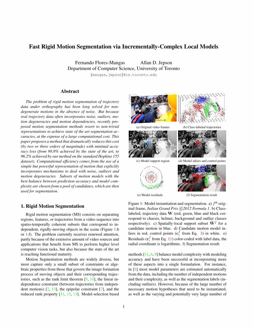
Figure 1: Model instantiation and segmentation. a) f th orig-inal frame, Italian Grand Prix c©2012 Formula 1. b) Class-labeled, trajectory data W (red, green, blue and black cor-respond to chassis, helmet, background and outlier classesrespectively). c) Spatially-local support subset Wf for acandidate motion in blue. d) Candidate motion model in-liers in red, control points (cfi from Eq. 3) in white. e)Residuals (rfi from Eq. 11) color-coded with label data, theradial coordinate is logarithmic. f) Segmentation result.

methods [11, 6, 8] balance model complexity with modelingaccuracy and have been successful at incorporating moreof these aspects into a single formulation. For instance,in [8] most model parameters are estimated automaticallyfrom the data, including the number of independent motionsand their complexity, as well as the segmentation labels (in-cluding outliers). However, because of the large number ofnecessary motion hypotheses that need to be instantiated,as well as the varying and potentially very large number of

1

model parameters that must be estimated, the flexibility of-fered by this method comes at a large computational cost.

Current state of the art methods follow the trend of us-ing sparse low-dimensional subspaces to represent trajec-tory data. This representation is then fed into a clusteringalgorithm to obtain a segmentation result. A prime exampleof this type of method is Sparse Subspace Clustering (SSC)[3] in which each trajectory is represented as a sparse linearcombination of a few other basis trajectories. The assump-tion is that the basis trajectories must belong to the samerigid motion as the reconstructed trajectory (or else, the re-construction would be impossible). When the assumptionis true, the sparse mixing coefficients can be interpreted asthe connectivity weights of a graph (or a similarity matrix),which is then (spectral) clustered to obtain a segmentationresult. At the time of publication, SSC produced segmenta-tion results three times more accurate than the best prede-cessor. The practical downside, however, is the inherentlylarge computational cost of finding the optimal sparse rep-resentation, which is at least cubic on the number of trajec-tories.

The work of [14] also falls within the class of subspaceseparation algorithms. Their approach is based on cluster-ing the principal angles (CPA) of the local subspaces associ-ated to each trajectory and its nearest neighbors. The clus-tering re-weights a traditional metric of subspace affinitybetween principal angles. Re-weighted affinities are thenused for segmentation. The approach produces segmenta-tion results with accuracies similar to those of SSC, but thecomputational cost is close to 10 times bigger than SSC’s.

In this work we argue that competitive segmentation re-sults are possible using a simple but powerful representationof motion that explicitly incorporates mechanisms to dealwith noise, outliers and motion degeneracies. The proposedmethod is approximately 2 or 3 orders of magnitude fasterthan [3] and [14] respectively, currently considered the stateof the art.

1.1. Affine Motion

Projective Geometry is often used to model the imagemotion of trajectories from rigid objects between pairs offrames. However, alternative geometric relationships thatfacilitate parameter computation have also been proven use-ful for this purpose. For instance, in perspective projection,general image motion from rigid objects can be modeledvia the composition of two elements: a 2D homography,and parallax residual displacements [5]. The homographydescribes the motion of an arbitrary plane, and the parallaxresiduals account for relative depths, that are unaccountedfor by the planar surface model.

Under orthography, in contrast, image motion of rigidobjects can be modeled via the composition of a 2D affinetransformation plus epipolar residual displacements. The

2D affine transformation models the motion of an arbitraryplane, and the epipolar residuals account for relative depths.Crucially, these two components can be computed sepa-rately and incrementally, which enables an explicit mech-anism to deal with motion degeneracy.

In the context of 3D motion, a motion is degenerate whenthe trajectories originate from a planar (or linear) object, orwhen neither the camera nor the imaged object exercise allof their degrees of freedom, such as when the object onlytranslates, or when the camera only rotates. These are com-mon situations in real world video sequences. The incre-mental nature of the decompositions described above, fa-cilitate the transition between degenerate motions and non-degenerate ones.

Planar Model Under orthography, the projection of tra-jectories from a planar surface can be modeled with theaffine transformation: xc

yc

1

=

[D t0> 1

] xw

yw

1

= Aw→c2D

xw

yw

1

, (1)

where D ∈ R2×2 is an invertible matrix, and t ∈ R2 isa translation vector. Trajectory coordinates (xw, yw) are inthe plane’s reference frame (modulo a 2D affine transfor-mation) and (xc, yc) are image coordinates.

Now, let W ∈ R2F×P be matrix of trajectory data thatcontains the x and y image coordinates of P feature pointstracked through F frames, as in

W =

x1,1 · · · x1,P

y1,1 · · · y1,P

.... . .

...xF,1 · · · xF,PyF,1 · · · yF,P

. (2)

To compute the parameters of A2D from trajectory data, letC = [c1, c2, c3] ∈ R2f×3 be three columns (three full tra-jectories) from W, and let cfi = [c2f−1

i , c2fi ]> be the x andy coordinates of the i-th control trajectory at frame f . Thenthe transformation between points from an arbitrary sourceframe s to a target frame f can be written as:[

cf1 cf2 cf31 1 1

]= As→f

2D

[cs1 cs2 cs31 1 1

], (3)

and As→f2D can be simply computed as:

As→f2D =

[cf1 cf2 cf31 1 1

] [cs1 cs2 cs31 1 1

]−1

. (4)

The inverse in the right-hand side matrix of Eq. 4 exists solong as the points csi are not collinear. For simplicity werefer to As→f

2D as Af2D and consequently As

2D is the identitymatrix.

3D Model In order to upgrade a planar (degenerate)model into a full 3D one, relative depth must be accountedusing the epipolar residual displacements. This means ex-tending Eq. 1 with a direction vector, scaled by the corre-sponding relative depth of each point, as in: xc

yc

1

=

[D ~t~0> 1

] xw

yw

1

+ δzw

a13

a23

0

. (5)

The depth δzw is relative to the arbitrary plane whose mo-tion is modeled by A2D; a point that lies on such planewould have δzw = 0. We call the orthographic version ofthe plane plus parallax decomposition, the 2D Affine PlusEpipolar (2DAPE) decomposition.

Eq. 5 is equivalent to

xc

yc

1

=

a11 a12 a13 t1a21 a22 a23 t20 0 0 1

xw

yw

δzw

1

(6)

where it is clear that the parameters of A3D define an or-thographically projected 3D affine transformation. Deter-mining the motion and structure parameters of a 3D modelfrom point correspondences can be done using the classicalmatrix factorization approach [10], but besides being sensi-tive to noise and outliers, the common scenario where thesolution becomes degenerate makes the approach difficultto use in real-world applications. Appropriately accommo-dating and dealing with the degenerate cases is one of thekey features of our work.

2. Overview of the MethodThe proposed motion segmentation algorithm has three

stages. First, a pool of M motion model hypothesesM ={M1, . . . ,MM} is generated using a method that combinesa Random Sampling and Consensus (RANSAC) [4] tech-nique with the 2DAPE decomposition. The goal is to gen-erate one motion model for each of the N independent,rigidly-moving objects in the scene; N is assumed to beknown a priori. The method instantiates many more mod-els than those expected necessary (M � N ) in an attemptincrease the likelihood of generating correct model propos-als for all N motions. A good model accurately describesa large subset of coherently moving trajectories with thesmallest number of parameters (§3).

In the second stage, subsets of motion models fromMare combined to explain all the trajectories in the sequence.The problem is framed as an objective function that mustbe minimized. The objective function is the negative log-likelihood over prediction accuracy, regularized by modelcomplexity (number of model parameters) and modelingoverlap (trajectories explained by multiple models). Notice

that after this stage, the segmentation that results from theoptimal model combination could be reported as a segmen-tation result (§5).

The third stage incorporates the results from a set ofmodel combinations that are closest to the optimal. Seg-mentation results are aggregated into an affinity matrix,which is then passed to a spectral clustering algorithm toproduce the final segmentation result. This refinement stagegenerally results in improved accuracy and reduced seg-mentation variability (§6).

3. Motion Model Instantiation

Each model M ∈ M is instantiated independently us-ing RANSAC. This choice is motivated because of thismethod’s well-known computational efficiency and robust-ness to outliers, but also because of its ability to incorpo-rate spatially local constraints and (as explained below) be-cause most of the computations necessary to evaluate a pla-nar model can be reused to estimate the likelihoods of apotentially necessary 3D model, yielding significant com-putational savings.

The input to our model instantiation algorithm is aspatially-local, randomly drawn subset of trajectory dataW[2F×I] ⊆ W[2F×P ] (§3.1). In turn, at each RANSACtrial, the algorithm draws uniformly distributed, randomsubsets of three control trajectories (C[2F×3] ⊂ W[2F×I]).Each set of control trajectories is used to estimate the fam-ily of 2D affine transformations {A1, . . . ,AF } between thebase frame and all other frames in the sequence, which arethen used to determine a complete set of model parametersM = {B,σ,C, ω}. The matrix B ∈ {0, 1}[F×I] indicateswhether the i-th trajectory should be predicted by modelM at frame f (inlier, bfi = 1) or not (outlier, bfi = 0),σ = {σ1, . . . , σF } are estimates of the magnitude of thenoise for each frame, and ω ∈ {2D, 3D} is the estimatedmodel type. The goal is to find the control points and theassociated parameters that minimize the objective function

O(W,M) =∑f∈F

∑i∈I

bfi Lω

(wf

i | Af , σf

)+ Ψ(ω) + Γ(B) (7)

across a number of RANSAC trials, where wfi =

(xfi , yfi ) = (w2f−1

i , w2fi ) are the coordinates of the i-th

trajectory from the support subset W at frame f . The neg-ative log-likelihood term Lω(·) penalizes reconstruction er-ror, while Ψ(·) and Γ(·) are regularizers. The three termsare defined below.

Knowing that 2D and 3D affine models have 6 and 8 de-grees of freedom respectively, Ψ(ω) regularizes over modelcomplexity using:

Ψ(ω) =

{6(F − 1), if ω = 2D8(F − 1), if ω = 3D.

(8)

Γ(B) strongly penalizes models that describe too fewtrajectories:

Γ(B) =

{∞, if

∑I

∑F b

fi < Fλi

0, otherwise(9)

The control set C whose M minimizes Eq. 7 across anumber of RANSAC trials becomes part of the pool of can-didatesM.

2D likelihoods. For the planar case (ω = 2D) the negativelog-likelihood term is evaluated with:

L2D(wfi | A

f , σf ) = − log

(1

2π|Σ|12

exp

{−

1

2rf>i Σ−1rfi

}),

(10)which is a zero-mean 2D Normal distribution evaluated atthe residuals rfi . The spherical covariance matrix is Σ =

(σf )2I. The residuals rfi are determined by the differencesbetween the predictions made by a hypothesized model Af ,and the observations at each frame[

rf

~1

]=

[wf

~1

]−Af

[ws

~1

]. (11)

3D likelihoods. The negative log-likelihood term for the3D case is based on the the 2DAPE decomposition. The2D affinities Af and residuals rf are reused, but to accountfor the effect of relative depth, an epipolar line segment ef

is robustly fit to the residual data at each frame (please seesupplementary material for details on the segment fitting al-gorithm). The 2DAPE does not constrain relative depths toremain constant across frames, but only requires trajectoriesto be close to the epipolar line. So, if the unitary vector ef⊥indicates the orthogonal direction to ef , then the negativelog-likelihood term for the 3D case is estimated with:

L3D(wfi | A

f , σf ) = −2 log

1√

2πσfexp

−(rf>i ef⊥

)2

2(σf )2

,

(12)which is also a zero-mean 2D Normal distribution com-puted as the product of two identical, separable, single-variate, normal distributions, evaluated at the distance fromthe residual to the epipolar line. The first one corresponds tothe actual deviation in the direction of ef⊥, which is analyti-cally computed using rf>i ef⊥. The second one correspondsto an estimate of the deviation in the perpendicular direc-tion (ef ), which cannot be determined using the 2DAPEdecomposition model, but can be approximated to be equalto rf>i ef⊥, which is a plausible estimate under the isotropicnoise assumption.

Note that Eq. 7 does not evaluate the quality of a modelusing the number of inliers, as it is typical for RANSAC.Instead, we found that better motion models resulted from

Algorithm 1: Motion model instantiationInput: Trajectory data W[2F×P ], number of RANSAC trialsK, arbitrary

base frame bOutput: Parameters of the motion model M = {B,σn, ω}

// determine the training set Wc← rand(1, P ); r ← rand(rmin, rmax) // random center and radiusW[2F×I] ← trajectoriesWithinDisk(W, r, c) // support subsetX← homoCoords(Wb) // points at base frame

forK RANSAC trials doc← rand3(1, I) // three random control trajectory indices

for f ∈ {1, . . . , F} − {b} doY ← homoCoords(Wf ) // points at frame fA← YcX

−1c // 2D affine model

R← AX−Y // residuals

[Bf2D, σ

f2D]← compute2DInliers(R)

Lf2D ← compute2DLikelihoods(R, σf

2D)[U, S, V ] = svd(weightedCov(R,B2D) // s1 ≥ s2if s1

s2> 1 + λ3D then

[Bf3D, σ

f3D]← compute3DInliers(R)

Lf3D ← compute3DLikelihoods(R, σf

3D)

// complete penalized neg-loglikleihoodsl2D ←

∑f

∑i B2D(f, i)L2D(f, i) + Ψ(2D) + Γ(B2D)

l3D ←∑

f

∑i B3D(f, i)L3D(f, i) + Ψ(3D) + Γ(B3D)

// keep the best model overallif (min(l2D, l3D) < l?) then

if (l2D < l3D) thenl? ← l2D;σ?

n ← σ2D;ω? ← 2;B? ← B2D

elsel? ← l3D;σ?

n ← σ3D;ω? ← 3;B? ← B3D

return M = {B?,σ?n, ω

?}

optimizing over the accuracy of the model predictions for an(estimated) inlier subset, which also means that the effect ofoutliers is explicitly uncounted.

Figure 1.b shows an example of class-labeled trajectorydata, 1.c shows a typical spatially-local support subset. Fig-ures 1.d and 1.e show a model’s control points and its corre-sponding (class-labeled) residuals, respectively. A pseudo-code description of the motion instantiation algorithm isprovided in Algorithm 1. Details on how to determine W,as well as B, σ, and ω follow.

3.1. Local Coherence

The subset of trajectories W given to RANSAC to gen-erate a model M is constrained to a spatially local region.The probability of choosing an uncontaminated set of 3 con-trol trajectories, necessary to compute a 2D affine model,from a dataset with a ratio r of inliers, after k trials is:p = 1 − (1 − r3)k. This means that the number of trialsneeded to find a subset of 3 inliers with probability p is

k =log(1− p)log(1− r3)

. (13)

A common assumption is that trajectories from the sameunderlying motion are locally coherent. Hence, a com-pact region is likely to increase r, exponentially reducing

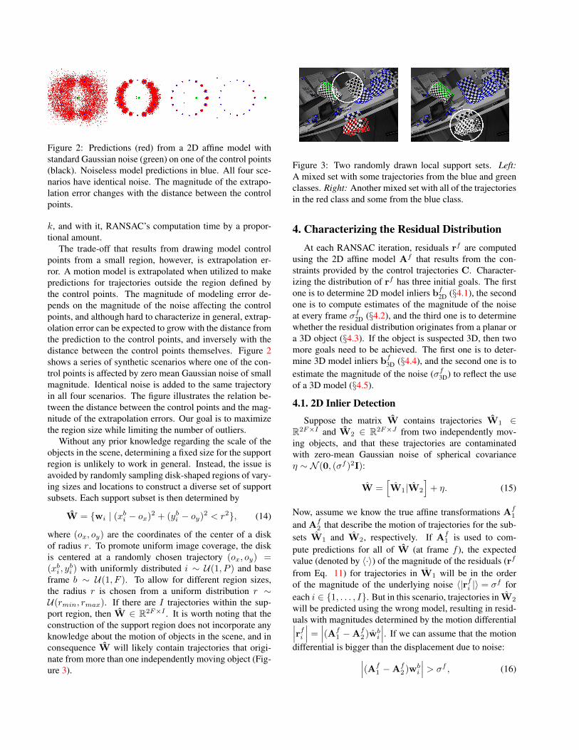
Figure 2: Predictions (red) from a 2D affine model withstandard Gaussian noise (green) on one of the control points(black). Noiseless model predictions in blue. All four sce-narios have identical noise. The magnitude of the extrapo-lation error changes with the distance between the controlpoints.

k, and with it, RANSAC’s computation time by a propor-tional amount.

The trade-off that results from drawing model controlpoints from a small region, however, is extrapolation er-ror. A motion model is extrapolated when utilized to makepredictions for trajectories outside the region defined bythe control points. The magnitude of modeling error de-pends on the magnitude of the noise affecting the controlpoints, and although hard to characterize in general, extrap-olation error can be expected to grow with the distance fromthe prediction to the control points, and inversely with thedistance between the control points themselves. Figure 2shows a series of synthetic scenarios where one of the con-trol points is affected by zero mean Gaussian noise of smallmagnitude. Identical noise is added to the same trajectoryin all four scenarios. The figure illustrates the relation be-tween the distance between the control points and the mag-nitude of the extrapolation errors. Our goal is to maximizethe region size while limiting the number of outliers.

Without any prior knowledge regarding the scale of theobjects in the scene, determining a fixed size for the supportregion is unlikely to work in general. Instead, the issue isavoided by randomly sampling disk-shaped regions of vary-ing sizes and locations to construct a diverse set of supportsubsets. Each support subset is then determined by

W = {wi | (xbi − ox)2 + (ybi − oy)2 < r2}, (14)

where (ox, oy) are the coordinates of the center of a diskof radius r. To promote uniform image coverage, the diskis centered at a randomly chosen trajectory (ox, oy) =(xbi , y

bi ) with uniformly distributed i ∼ U(1, P ) and base

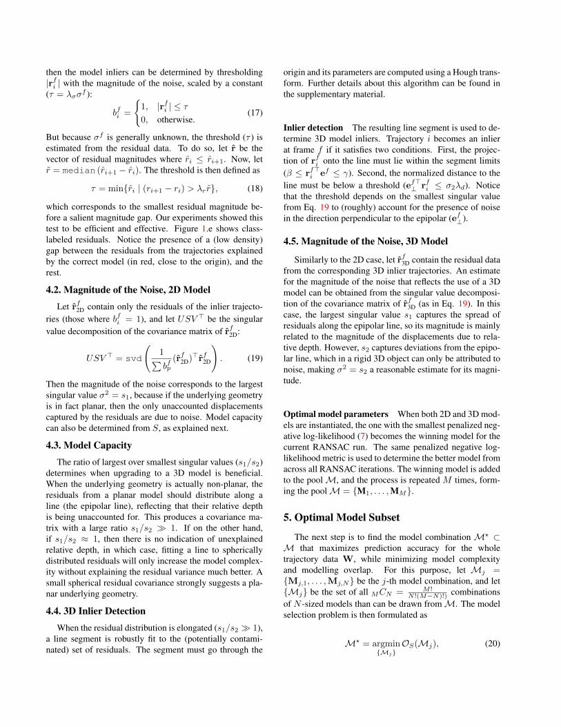
frame b ∼ U(1, F ). To allow for different region sizes,the radius r is chosen from a uniform distribution r ∼U(rmin, rmax). If there are I trajectories within the sup-port region, then W ∈ R2F×I . It is worth noting that theconstruction of the support region does not incorporate anyknowledge about the motion of objects in the scene, and inconsequence W will likely contain trajectories that origi-nate from more than one independently moving object (Fig-ure 3).

Figure 3: Two randomly drawn local support sets. Left:A mixed set with some trajectories from the blue and greenclasses. Right: Another mixed set with all of the trajectoriesin the red class and some from the blue class.

4. Characterizing the Residual DistributionAt each RANSAC iteration, residuals rf are computed

using the 2D affine model Af that results from the con-straints provided by the control trajectories C. Character-izing the distribution of rf has three initial goals. The firstone is to determine 2D model inliers bf2D (§4.1), the secondone is to compute estimates of the magnitude of the noiseat every frame σf2D (§4.2), and the third one is to determinewhether the residual distribution originates from a planar ora 3D object (§4.3). If the object is suspected 3D, then twomore goals need to be achieved. The first one is to deter-mine 3D model inliers bf3D (§4.4), and the second one is toestimate the magnitude of the noise (σf3D) to reflect the useof a 3D model (§4.5).

4.1. 2D Inlier Detection

Suppose the matrix W contains trajectories W1 ∈R2F×I and W2 ∈ R2F×J from two independently mov-ing objects, and that these trajectories are contaminatedwith zero-mean Gaussian noise of spherical covarianceη ∼ N (0, (σf )2I):

W =[W1|W2

]+ η. (15)

Now, assume we know the true affine transformations Af1

and Af2 that describe the motion of trajectories for the sub-

sets W1 and W2, respectively. If Af1 is used to com-

pute predictions for all of W (at frame f ), the expectedvalue (denoted by 〈·〉) of the magnitude of the residuals (rf

from Eq. 11) for trajectories in W1 will be in the orderof the magnitude of the underlying noise 〈|rfi |〉 = σf foreach i ∈ {1, . . . , I}. But in this scenario, trajectories in W2

will be predicted using the wrong model, resulting in resid-uals with magnitudes determined by the motion differential∣∣∣rfi ∣∣∣ =

∣∣∣(Af1 −Af

2 )wbi

∣∣∣. If we can assume that the motiondifferential is bigger than the displacement due to noise:∣∣∣(Af

1 −Af2 )wb

i

∣∣∣ > σf , (16)

then the model inliers can be determined by thresholding|rfi | with the magnitude of the noise, scaled by a constant(τ = λσσ

f ):

bfi =

{1, |rfi | ≤ τ0, otherwise.

(17)

But because σf is generally unknown, the threshold (τ ) isestimated from the residual data. To do so, let r be thevector of residual magnitudes where ri ≤ ri+1. Now, letr = median (ri+1 − ri). The threshold is then defined as

τ = min{ri | (ri+1 − ri) > λr r}, (18)

which corresponds to the smallest residual magnitude be-fore a salient magnitude gap. Our experiments showed thistest to be efficient and effective. Figure 1.e shows class-labeled residuals. Notice the presence of a (low density)gap between the residuals from the trajectories explainedby the correct model (in red, close to the origin), and therest.

4.2. Magnitude of the Noise, 2D Model

Let rf2D contain only the residuals of the inlier trajecto-ries (those where bfi = 1), and let USV > be the singularvalue decomposition of the covariance matrix of rf2D:

USV > = svd

(1∑bfp

(rf2D)>rf2D

). (19)

Then the magnitude of the noise corresponds to the largestsingular value σ2 = s1, because if the underlying geometryis in fact planar, then the only unaccounted displacementscaptured by the residuals are due to noise. Model capacitycan also be determined from S, as explained next.

4.3. Model Capacity

The ratio of largest over smallest singular values (s1/s2)determines when upgrading to a 3D model is beneficial.When the underlying geometry is actually non-planar, theresiduals from a planar model should distribute along aline (the epipolar line), reflecting that their relative depthis being unaccounted for. This produces a covariance ma-trix with a large ratio s1/s2 � 1. If on the other hand,if s1/s2 ≈ 1, then there is no indication of unexplainedrelative depth, in which case, fitting a line to sphericallydistributed residuals will only increase the model complex-ity without explaining the residual variance much better. Asmall spherical residual covariance strongly suggests a pla-nar underlying geometry.

4.4. 3D Inlier Detection

When the residual distribution is elongated (s1/s2 � 1),a line segment is robustly fit to the (potentially contami-nated) set of residuals. The segment must go through the

origin and its parameters are computed using a Hough trans-form. Further details about this algorithm can be found inthe supplementary material.

Inlier detection The resulting line segment is used to de-termine 3D model inliers. Trajectory i becomes an inlierat frame f if it satisfies two conditions. First, the projec-tion of rfi onto the line must lie within the segment limits(β ≤ rf>i ef ≤ γ). Second, the normalized distance to theline must be below a threshold (ef>⊥ rfi ≤ σ2λd). Noticethat the threshold depends on the smallest singular valuefrom Eq. 19 to (roughly) account for the presence of noisein the direction perpendicular to the epipolar (ef⊥).

4.5. Magnitude of the Noise, 3D Model

Similarly to the 2D case, let rf3D contain the residual datafrom the corresponding 3D inlier trajectories. An estimatefor the magnitude of the noise that reflects the use of a 3Dmodel can be obtained from the singular value decomposi-tion of the covariance matrix of rf3D (as in Eq. 19). In thiscase, the largest singular value s1 captures the spread ofresiduals along the epipolar line, so its magnitude is mainlyrelated to the magnitude of the displacements due to rela-tive depth. However, s2 captures deviations from the epipo-lar line, which in a rigid 3D object can only be attributed tonoise, making σ2 = s2 a reasonable estimate for its magni-tude.

Optimal model parameters When both 2D and 3D mod-els are instantiated, the one with the smallest penalized neg-ative log-likelihood (7) becomes the winning model for thecurrent RANSAC run. The same penalized negative log-likelihood metric is used to determine the better model fromacross all RANSAC iterations. The winning model is addedto the poolM, and the process is repeated M times, form-ing the poolM = {M1, . . . ,MM}.

5. Optimal Model Subset

The next step is to find the model combination M? ⊂M that maximizes prediction accuracy for the wholetrajectory data W, while minimizing model complexityand modelling overlap. For this purpose, let Mj ={Mj,1, . . . ,Mj,N} be the j-th model combination, and let{Mj} be the set of all MCN = M !

N !(M−N)!) combinationsof N -sized models than can be drawn fromM. The modelselection problem is then formulated as

M? = argmin{Mj}

OS(Mj), (20)

where the objective is

OS(Mj) =

N∑n=1

P∑p=1

πp,nE (wp,Mj,n)

+ λΦ

P∑i=1

Φ(wp,Mj,n) + λΨ

N∑n=1

Ψ(Mj,n).

(21)

The first term accounts for prediction accuracy, the othertwo are regularization terms. Details follow.

Prediction Accuracy In order to determine how well amodel M predicts an arbitrary trajectory w, the affine trans-formations estimated by RANSAC could be re-used. How-ever, the inherent noise in the control points, and the po-tentially short distance between them, often render this ap-proach impractical, particularly when w is spatially distantfrom the control points (see §3.1). Instead, model parame-ters are computed with a factorization based [10] method.Given the inlier labeling B in M, let WB be the subset oftrajectories where bfi = 1 for at least half of the frames. Theorthonormal basis S of a ω = 2D (or 3D) motion model canbe determined by the 2 (or 3) left singular vectors of WB.Using S as the model’s motion matrices, prediction accu-racy can be computed using:

E(w,M) =∣∣SS>w −w

∣∣2 , (22)

which is the sum of squared Euclidean deviations from thepredictions (SS>w), to the observed data (w). Our exper-iments indicated that, although sensitive to outliers, thesemodel predictions are much more robust to noise.

Ownership variables Π ∈ {0, 1}[P×N ] indicate whethertrajectory p is explained by the n-th model (πp,n = 1) ornot (πp,n = 0), and are determined by maximum predictionaccuracy (i.e. minimum Euclidean deviation):

πp,n =

1, if Mj,n = argminM∈Mj

E(wp,M)

0, otherwise.(23)

Regularization terms The second term from Eq. 21 pe-nalizes situations where multiple models explain a trajec-tory (w) with relatively small residuals. For brevity, letE(w,M) = exp{−E(w,M)}, then:

Φ(w,Mj) = − log

maxM∈Mj

E(w,M)∑M∈Mj

E(w,M). (24)

The third term regularizes over the number of model param-eters, and is evaluated using Eq. 8. The constants λΦ andλΨ modulate the effect of the corresponding regularizer.

Table 1: Accuracy and run-time for the H155 dataset. NaiveRANSAC included as a baseline with overall accuracy andtotal computation time estimated using data from [12].

Algorithm Average Accuracy [%] Computation time [s]SSC [3] 98.76 14500CPA [14] 98.75 147600RANSAC 89.15 30Ours 96.19 217

6. RefinementThe optimal model subset M? yields ownership vari-

ables Π? which can already be interpreted as a segmenta-tion result. However, we found that segmentation accuracycan be improved by incorporating the labellings Πt fromthe top T subsets {M?

t | 1 ≤ t ≤ T} closest to optimal.Multiple labellings are incorporated into an affinity ma-

trix F, where the fi,j entry indicates the frequency withwhich trajectory i is given the same label as trajectory jacross all T labellings, weighted by the relative objectivefunction Ot = exp

{−OS(W|M?

t )OS(W|M?)

}for such a labelling:

fi,j =1∑T

t=1 Ot

T∑t=1

(πti,:π

t>j,:

)Ot (25)

Note that the inner product between the label vectors(πi,:π

>j,:) is equal to one only when the labels are the same.

A spectral clustering method is applied on F to producethe method’s final segmentation result.

7. ExperimentsEvaluation was made through three experimental setups.

Hopkins 155 The Hopkins 155 (H155) dataset has beenthe standard evaluation metric for the problem of motionsegmentation of trajectory data since 2007. It consists ofcheckerboard, traffic and articulated sequences with either 2or 3 motions. Data was automatically tracked, but trackingerrors were manually corrected; further details are availablein [12]. The use of a standard dataset enables direct compar-ison of accuracy and run-time performance. Table 1 showsthe relevant figures for the two most competitive algorithmsthat we are aware of. The data indicates that our algorithmhas run-times that are close to 2 or 3 orders of magnitudefaster than the state of the art methods, with minimal ac-curacy loss. Computation times are measured in the same(or very similar) hardware architectures. Like in CPA, ourimplementation uses a single set of parameters for all theexperiments, but as others had pointed out [14], it remainsunclear whether the same is true for the results reported inthe original SSC paper.

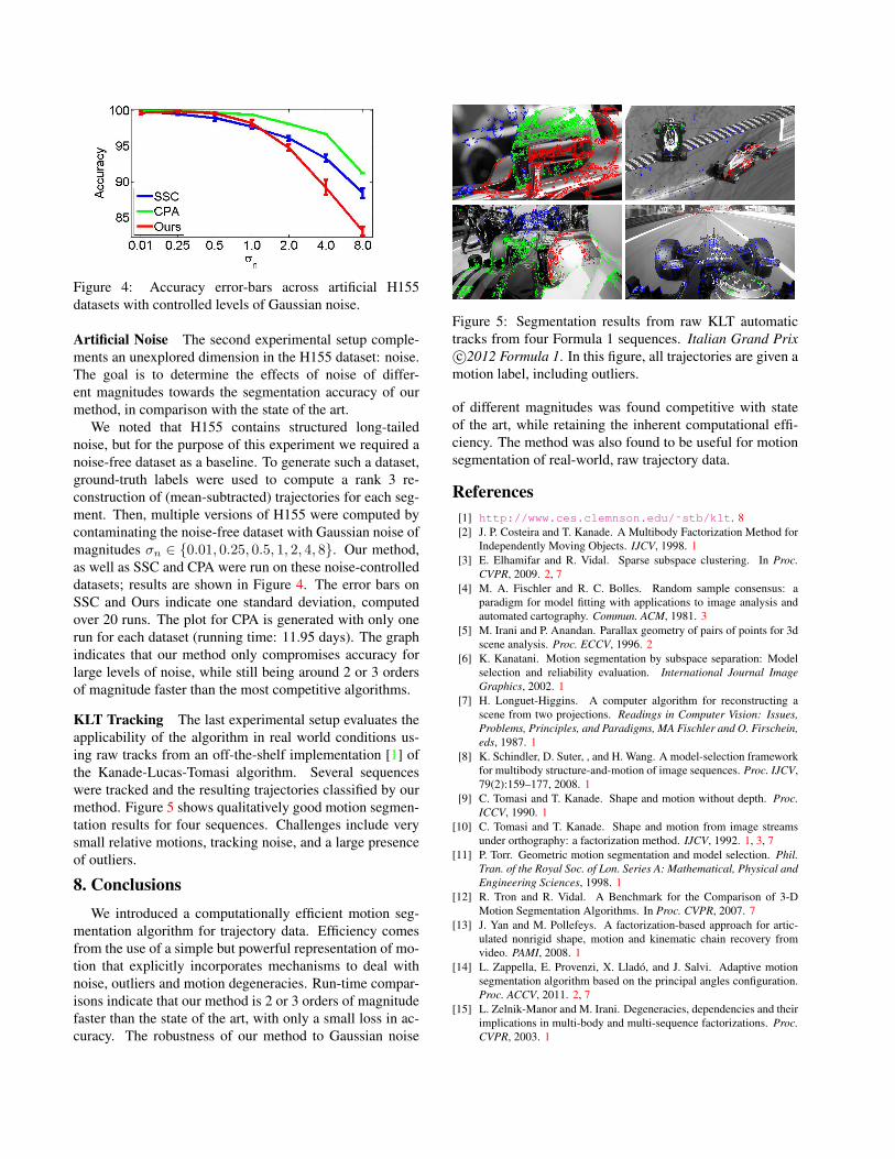
Figure 4: Accuracy error-bars across artificial H155datasets with controlled levels of Gaussian noise.

Artificial Noise The second experimental setup comple-ments an unexplored dimension in the H155 dataset: noise.The goal is to determine the effects of noise of differ-ent magnitudes towards the segmentation accuracy of ourmethod, in comparison with the state of the art.

We noted that H155 contains structured long-tailednoise, but for the purpose of this experiment we required anoise-free dataset as a baseline. To generate such a dataset,ground-truth labels were used to compute a rank 3 re-construction of (mean-subtracted) trajectories for each seg-ment. Then, multiple versions of H155 were computed bycontaminating the noise-free dataset with Gaussian noise ofmagnitudes σn ∈ {0.01, 0.25, 0.5, 1, 2, 4, 8}. Our method,as well as SSC and CPA were run on these noise-controlleddatasets; results are shown in Figure 4. The error bars onSSC and Ours indicate one standard deviation, computedover 20 runs. The plot for CPA is generated with only onerun for each dataset (running time: 11.95 days). The graphindicates that our method only compromises accuracy forlarge levels of noise, while still being around 2 or 3 ordersof magnitude faster than the most competitive algorithms.

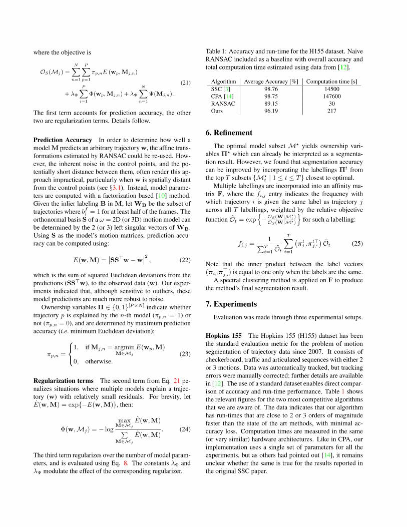
KLT Tracking The last experimental setup evaluates theapplicability of the algorithm in real world conditions us-ing raw tracks from an off-the-shelf implementation [1] ofthe Kanade-Lucas-Tomasi algorithm. Several sequenceswere tracked and the resulting trajectories classified by ourmethod. Figure 5 shows qualitatively good motion segmen-tation results for four sequences. Challenges include verysmall relative motions, tracking noise, and a large presenceof outliers.

8. ConclusionsWe introduced a computationally efficient motion seg-

mentation algorithm for trajectory data. Efficiency comesfrom the use of a simple but powerful representation of mo-tion that explicitly incorporates mechanisms to deal withnoise, outliers and motion degeneracies. Run-time compar-isons indicate that our method is 2 or 3 orders of magnitudefaster than the state of the art, with only a small loss in ac-curacy. The robustness of our method to Gaussian noise

Figure 5: Segmentation results from raw KLT automatictracks from four Formula 1 sequences. Italian Grand Prixc©2012 Formula 1. In this figure, all trajectories are given a

motion label, including outliers.

of different magnitudes was found competitive with stateof the art, while retaining the inherent computational effi-ciency. The method was also found to be useful for motionsegmentation of real-world, raw trajectory data.

References[1] http://www.ces.clemnson.edu/˜stb/klt. 8[2] J. P. Costeira and T. Kanade. A Multibody Factorization Method for

Independently Moving Objects. IJCV, 1998. 1[3] E. Elhamifar and R. Vidal. Sparse subspace clustering. In Proc.

CVPR, 2009. 2, 7[4] M. A. Fischler and R. C. Bolles. Random sample consensus: a

paradigm for model fitting with applications to image analysis andautomated cartography. Commun. ACM, 1981. 3

[5] M. Irani and P. Anandan. Parallax geometry of pairs of points for 3dscene analysis. Proc. ECCV, 1996. 2

[6] K. Kanatani. Motion segmentation by subspace separation: Modelselection and reliability evaluation. International Journal ImageGraphics, 2002. 1

[7] H. Longuet-Higgins. A computer algorithm for reconstructing ascene from two projections. Readings in Computer Vision: Issues,Problems, Principles, and Paradigms, MA Fischler and O. Firschein,eds, 1987. 1

[8] K. Schindler, D. Suter, , and H. Wang. A model-selection frameworkfor multibody structure-and-motion of image sequences. Proc. IJCV,79(2):159–177, 2008. 1

[9] C. Tomasi and T. Kanade. Shape and motion without depth. Proc.ICCV, 1990. 1

[10] C. Tomasi and T. Kanade. Shape and motion from image streamsunder orthography: a factorization method. IJCV, 1992. 1, 3, 7

[11] P. Torr. Geometric motion segmentation and model selection. Phil.Tran. of the Royal Soc. of Lon. Series A: Mathematical, Physical andEngineering Sciences, 1998. 1

[12] R. Tron and R. Vidal. A Benchmark for the Comparison of 3-DMotion Segmentation Algorithms. In Proc. CVPR, 2007. 7

[13] J. Yan and M. Pollefeys. A factorization-based approach for artic-ulated nonrigid shape, motion and kinematic chain recovery fromvideo. PAMI, 2008. 1

[14] L. Zappella, E. Provenzi, X. Llado, and J. Salvi. Adaptive motionsegmentation algorithm based on the principal angles configuration.Proc. ACCV, 2011. 2, 7

[15] L. Zelnik-Manor and M. Irani. Degeneracies, dependencies and theirimplications in multi-body and multi-sequence factorizations. Proc.CVPR, 2003. 1