Fast Pattern Recognition using Normalized Grey-Scale

Machine Vision & Applications manuscript No.(will be inserted by the editor)

Fast Pattern Recognition using Normalized

Grey-Scale Correlation in a Pyramid Image

Representation

W. James MacLean1, John K. Tsotsos2

1 University of Toronto, Department of Electrical & ComputerEngineering, Toronto, Canada M5S 1A1

2 York University, Department of Computer Science, Toronto,Canada M3J 1P3

February 16, 2007

Abstract The ability to quickly locate one or more instances of a modelin a

grey scale image is of importance to industry. The recognition/ localization must

be fast and accurate. In this paper we present an algorithm which incorporates nor-

malized correlation into a pyramid image representation structure to perform fast

recognition and localization. The algorithm employs an estimate of the gradient of

the correlation surface to perform a steepest descent search. Test results are given

detailing search time by target size, effect of rotation andscale changes on perfor-

mance, and accuracy of the subpixel localization algorithmused in the algorithm.

Finally, results are given for searches on real images with perspective distortion

and the addition of Gaussian noise.

Send offprint requests to: W. James MacLean

2 W. James MacLean, John K. Tsotsos

1 Introduction

Fast pattern recognition is an invaluable component of manymachine-vision al-

gorithms used in industry today. The ability to quickly identify an object, or a

marking on an object can aid in finding a desired part among a group of parts, or

to register a part so that work may be performed on it. This paper outlines an algo-

rithm for fast detection and localization of a pattern usingsimple and inexpensive

hardware. For example, typical search times are less than 0.25 S, and as low as 10–

30 mS when the expected number of targets is known in advance.1 Specifically, the

algorithm is suitable for implementation on a personal computer equipped with an

image acquisition board and a camera.

The algorithm relies on a pyramid representation of both themodel image

and the search image, as well as an estimate of the gradient ofthe correlation

surface. The algorithm begins by creating a pyramid representation of the model

image. A worst-case analysis is then used to determine the effect on the correlation

score of i) the number of pyramid levels combined with ii) thepossible different

registrations of the pyramid sampling grid with respect to the model, in order to

determine the optimum number of pyramid levels to use. This analysis is done

once off-line.

During the search phase, a pyramid representation is built from the image be-

ing searched for instances of the model. It is built to the same depth as the model

pyramid. The top-level of the model pyramid is convolved with the top-level of

the search-image pyramid to produce a correlation surface from which likely can-

1 These times are reported for a 750 MHz Athlon processor.

Fast NGC Pattern Recognition in an Image Pyramid 3

didates for model instances can be chosen. For each candidate, the search pro-

cess descends through the pyramid performing a steepest descent search based on

the correlation-gradient at each level. When the bottom level is reached, either a

model instance has been found or the candidate is rejected for failing to meet a

minimum threshold for its correlation score. Once a model instance is found, a

bi-quadratic sub-pixel localization algorithm can be applied if desired. Figure 1

shows an overview of the search algorithm.

Correlation does not generally allow for size or rotationalorientation varia-

tions, nor does it allow for model instances which are partially occluded. Non-

uniform lighting variations will also detract from the algorithm’s performance,

but it is assumed that these may be controlled in industrial settings. Despite these

drawbacks inherent in correlation-based matching, our algorithm is suitable for

incorporation into larger algorithms that address the issues of size and rotation

variance, possibly through the use of multiple search templates giving information

about a target in different sizes and orientations. It is also suitable for extending

matching methods based on principal components analysis (PCA), such as those

found in [37,26].

An outline of this paper is as follows: results of previous approaches are con-

sidered in section 2. Section 3 deals with the idea of performing normalized grey-

scale correlation in a pyramid structure. Section 3.1 develops an estimate of the

correlation gradient for gradient-descent search. An important feature of this esti-

mate is that it can be computed quickly. In section 3.3 a method for choosing the

depth of the pyramid is presented. Section 4 describes details of the algorithm’s


implementation and gives performance results. A discussion of the results of ap-

plying the algorithm are presented in section 5.

2 Review of Previous Work

The problem of finding targets in images involves two important steps:localization

of candidate matches within the image, and verification of each candidate through

a matchingprocess. Most of the relevant literature in the field involves the task of

matching, and as such assumes that the images being comparedare of the same

size. Matching algorithms can be broken down into two major categories, those

based on correlation and those based on features. The lattercategory includes fea-

tures based on colour, gradient orientation, moments and shape descriptors. Match-

ing algorithms often ignore issues related to scale and orientation, leaving those to

be determined during the localization stage. The task of localization involves find-

ing the right region within the search image (including determining the region’s

size) and passing this region to the verification process.

Some of the earliest attempts at matching have been done using correlation

methods, which are reviewed in detail in [10,29,5]. The concept of normalized

correlation was developed to combat the effect of differentillumination levels

on these techniques. A major downfall of correlation techniques is that, when

combined with naive localization methods such as brute-force search, they are

computationally very intensive, and as such tend to be slow.Despite this, they

have remained popular with the advent of appearance-based matching methods

such as eigenfaces and related techniques [37,26]. Anotherclass of techniques in-


volves matching moments [29], but is limited to the case where localization has

already been performed, and the pattern to be matched has been segmented from

the background prior to applying the moment operators. Whenthis can be done

these techniques are often powerful, as they can provide rotation and size invariant

recognition [11,6], although the issue of localization is seldom addressed. Other

moment-based approaches include [13,41,15], with the latter using Zernicke mo-

ments computed using polar coordinates.

Combining an approach similar to correlation with feature-type matching, both

[27,13] use deformable templates to match models to target instances. In [13] the

matching is performed on candidates retrieved using feature vector indexing. The

amount of warp and discrepancy in the resulting edge maps is used as a measure

of similarity to rank the top matches. Matches are performedon binary images.

Nastaret. al.[27] performs image matching using pixel intensities in a method de-

scribed as a generalization of optic flow and eigenfaces. Also based on deformable

templates, a description is given in [31] of a search technique which is somewhat

robust to scale changes and moderate rotation about the vertical axis. The tech-

nique involves dividing the target into columns, and allowing pixels from each

column to match one or more columns in the search image using adynamic pro-

gramming method. Robustness to moderate scale change is provided by searching

over three pre-defined scales in the search image. While it isclaimed that this

technique is superior to NGC (normalized grey-scale correlation), no timing com-

parison is done.


There exist a number of techniques for matching entire images [28,33,13,41].

These techniques typically generate indices to allow fast retrieval of similar im-

ages from a database, and they often assume that images have been normalized in

size. In [28] appearance-based matching is used to index into a database of im-

ages. This work is largely based on eigen-image matching with a Karhunen-Loeve

transformation to limit the size of the basis space required. In a method similar to

work reported later in [27], shape matching based on eigenmodes is also used to

index into the database.

One class of approaches to matching is based on extracting features from

the images under consideration. Two popular features are colour [4,33,41] and

edge orientation [33,18,13]. Colour features usually involve matching colour his-

tograms over the region of interest, but they are only applicable to colour images.

In [33] a technique for indexing images based on both colour and edge-orientation

histograms is given, with the intent of matching via nearestneighbour techniques.

Similarly [13] uses colour histograms with moment invariants as an indexing fea-

ture to find top candidates for subsequent matching with deformable templates. In

[4] the authors present a colour histogram matching metric,and demonstrate its

usefulness by finding Waldo in images from the popular “Where’s Waldo?” series.

Since the histograms are computed over local regions of fixedsize, the technique is

not only able to detect Waldo but also find his location. In [41] colour histograms

are combined with Fourier, moment-invariants and intensity projection ontox and

y axes to provide a means for indexing into a trademark database. Both [33,13]

use edge orientation histograms to provide indexing for matching. In a different


vein, Lowe [18,19] computes local features based on magnitude and orientation

information at image regions determined to have stable responses to a difference-

of-Gaussians filter, across multiple scales. The novel aspect of this work is that

it matches features in the target to features in a search image based on a Hough

transform for accumulating pose parameters. This estimation of pose parameters

seeks to solve localization as well as matching. This methodis better described as

a parts-based object recognition scheme, even though no semantics are attached

to individual features. The performance is fast (estimatedto be on the order of

100 mS or better on modern hardware), and is tolerant to scaling and rotation in,

and to some extent out, of the image plane. The features used are, however, sen-

sitive to global changes in illumination [3], unlike normalized correlation. Lowe’s

technique is not expected to be easily applied to small targets, for example an8×8

target, as it will be difficult to assess stability across scales since details will disap-

pear quickly as coarser scales are attempted. Further, thismethod does not appear

to be suitable for sub-pixel localization of the target. A number of affine-invariant

feature detection techniques have been developed in recentyears [1,21–23,25,24].

Maximally-stable extremal regions (MSER) [1] is a technique that identifies re-

gions based on their stability when thresholded using a range of thresholds. These

stable regions are considered features, and suitable descriptors can be used to de-

scribe their content. A number of affine-invariant descriptors [21–23] are based on

applying the standard Harris-Stephens corner detector [9]across multiple scales

to find a maximal response, and computing an elliptical region around the fea-

ture location whose scale and orientation can be used to created an affine-invariant


descriptor for the feature. These descriptors, like SIFT descriptors, are useful for

comparing features across different images and across different scales and orien-

tations. These techniques have proven useful in content-based image retrieval and

indexing in video sequences [35], using the “bag of features” concept. Any of the

techniques involving image gradients may run into problemsfor artificial images

with high contrast and considerable regularity in edge orientations, for example

corporate logos.

Another feature approach involves the use of probabilisticfeatures [32,36]. In

[32] object appearance is encoded using estimates of joint density functions for the

recovered features. While this system is fast (on the order of 100 mS on an SGI

O2 workstation), it is only intended for detection and not localization (localization

accuracy is 30 to 80 pixels). Stauffer & Grimson [36] use a setof training images

of the target to learn a joint distribution of pixel intensities in an image patch.

Comparison of the joint density to that of a candidate image patch takes about

1 second on a 500 MHz pentium, making the method too slow for fast object

localization.

A new class of technique is centred around neural networks, but to date they

are more suited to pattern classification than localization. Kulkarni [16] describes

a size/rotation invariant object recognition method usingback propagation to rec-

ognize feature vectors, but the vectors are based on momentsand thus are good

for matching but not localization. Work done by Wechsler & Zimmerman [39,40]

looks more promising, but seems too complex to be fast on modest hardware. In

[12] neural networks are used to learn optimal templates fornearest neighbour


matching. In [41] a neural network is used to classify based on recovered feature

vectors.

Finally, the concept of using pyramid representations for image analysis is

certainly not new, and is closely linked to the theory of scale-space [14,17]. In

this paper pyramid representations are used to overcome some of the computa-

tional problems associated with correlation methods. Burt[2] has constructed a

pyramid-based attention model which uses Gaussian and Laplacian pyramids, and

which is used for foveation, tracking and determining whereto look next based on

image saliency. Their system can be used for pattern recognition by using a pat-

tern tree to represent salient features of objects at different resolutions. If enough

features are matched, then the pattern has been found. Special hardware has been

developed [38] to aid in the construction of image pyramids.Lowe [18] uses mul-

tiple image scales to determine the stability of features. Ramapriyanet al. [30]

uses a multi-level decision tree approach to finding templates in images. A set of

target templates is partitioned in a manner that allows subsets of templates to be

removed from consideration should initial computations ata particular image lo-

cation contraindicates. If evidence supports further search, the candidates under

consideration is narrowed until a best match occurs. Since only a small number of

matches are expected over the large number of possible imagelocations, search

speed is greatly improved. In [7] Greenspan proposes a decision tree method for

determining 3-D object pose in images, again making use of hierarchical search in

pattern matching.


Worst CaseAnalysis

Image Pyramid

Top−LevelCorrelation

CandidateSelection

Search Image Model Image

Model Pyramid

Candidatefound?

pyramidsize

Yes

No

Yes

End

MultiscaleSearch

Abovethresh

No

YesNo

Max Targets?

Min Top−Level Score

SubpixelEstimation> 0?

level

YesNo

Pre

−pr

oces

sing

Fig. 1 Overview of pyramid-based NGC search.

3 NGC in a Pyramid Representation

This section describes the use of a pyramid image representation to reduce the

computational complexity associated with correlation search. LetI(x, y) represent

an imageIw × Ih pixels in size. The top-left corner of the image is defined to be

the origin. Each pixel is assumed to encode a grey value in therange0 . . . 255, one

byte per pixel, although colour correlation is easily achieved by replacing pixel

multiplications with inner-product operations performedon RGB values repre-

sented as vectors. If we wish to use correlation to search fora modelM(x, y)

of sizeMw × Mh in the image, the complexity for performing the correlationis

O(IwIhMwMh). However, the cost of the computation increases considerably if

normalized correlation is used (see Eq. 1).

C(x, y) =G(M(0, 0), I(x, y))

√

G(M(0, 0), M(0, 0))G(I(x, y), I(x, y)), (1)


where

G(f1(x1, y1), f2(x2, y2)) =

Mw−1∑

i=0

Mh−1∑

j=0

f1(x1 + i, y1 + j)f2(x2 + i, y2 + j)

andx < Iw − Mw + 1 andy < Ih − Mh + 1.

An overview of the method is as follows: build pyramid representations of

both the model and the image (search space), and perform correlation search at the

top levels of the two pyramids. This can be done very quickly due to the reduced

image sizes. The best match at the top level can be refined using a coarse-to-fine

strategy in which the best estimate of location at levelk in the pyramid is used

as the starting point for the search at levelk − 1. When the base of the pyramid

is reached, the model has been found. Multiple instances canbe found through

repeating this procedure by choosing more than one match at the top level of the

pyramid.

We now describe briefly the method of building both the image pyramid and

the model pyramid. The structure of the pyramid is quite simple. We have used an

averaging-with-no-overlap scheme, and use a sub-samplingrate of2. This means

that each level in the pyramid has dimensions equal to one-half of those for the

level below, meaning that each level is one-quarter the sizeof the one immediately

below. Each pixel in a given layer is the average of four pixels from the layer be-

low. These four pixels are termed the receptive field of the pixel on the higher level,

and the fact that the pyramid is non-overlapped means that oneach level the re-

ceptive fields do not overlap each other. This type of pyramidcan be built quickly,

as each pixel in a new level only requires 3 adds and one shift to compute. The

algorithm for building the pyramid isO(IwIh). The number of levels is limited


Fig. 2 The pyramid representation for a typical image is shown. Thepyramid has three

levels, with level 0 being the largest image at320×240 (top), and level 2 being the smallest

at80 × 60 (bottom right). In the level 0 image, a search model is defined.

by Kmax ≤ log2 min(Mw, Mh). The advantages of building a pyramid become

quickly obvious: theKth-level of a pyramid has22(K−1) times fewer pixels than

does the original image. Remember that the model pyramid at level K also has

22(K−1) times fewer pixels than at its level 0, so that the total cost of NGC at the

top level of the pyramid is24(K−1) times smaller than NGC on the original image.

For a 4-level pyramid, this factor is 4096.

To perform correlation search for the model at the top-levelof the pyramid,

the complexity isO((IwIhMwMh)/24(K−1)). Of course, the localization of the


Fig. 3 The pyramid representation of the model in Figure 2 is shown.It has the same

number of levels as the image pyramid.

pattern at the top level of the pyramid is not perfect, but this can be used as an

initial estimate for the next level of the pyramid. At each level of the pyramid a

small number of correlations is used to refine the location estimate.

Instead of performing an exhaustive local search for the newmaximum at each

level of the pyramid, it is possible to estimate the gradientof the correlation surface

and use a steepest descent method to perform the search. The following section

describes the derivation of the gradient estimate.

3.1 Derivation of Correlation Gradient

When the estimate of model location is refined at each level ofthe pyramid, it is

possible to use an estimate of the gradient of the correlation surface to perform

a steepest descent search. While it is possible to estimate the correlation surface

in a 3 × 3 neighbourhood centred on the current location estimate, this is com-

putationally expensive (it requires 9 full correlations).It is possible to estimate

the correlation gradient in a less expensive manner. However, in applying steepest

descent to a surface that we expect will have multiple maxima, it is important to


identify regions expected to contain local maxima to allow the search to converge

quickly. The use of the image pyramid does this: not only doesit limit complexity

of the top-level correlation, but it facilitates finding candidate regions and pro-

vides a means of quickly refining the search. In the derivation which follows the

continuous case is developed: the transition to the discrete case is straighforward.

Given an imageI(x, y) and a modelM(x, y), with M being differentiable

over allx andy, the correlation coefficient surface can be defined as

C(u, v) =

∫

∞

∞

∫

∞

∞I(x, y)(MW )(x − u, y − v)dx dy

[∫

∞

∞

∫

∞

∞I2(x, y)W (x − u, y − v)dx dy

]1/2. (2)

(Note: the integration limits in subsequent equations are the same, but are omit-

ted for compactness of notation.) The functionW (x, y) is a windowing function

which is used to force the contribution fromM to zero at its boundaries:

W (x, y) = 0 ∀ x < 0, x > Mw, y < 0 and y > Mh . (3)

The notation(MW )(x, y) is shorthand forM(x, y)W (x, y). For simple correla-

tion computation,W is normally chosen to be a box function. However, since we

will want to differentiate Eq. 2, the windowing function should be chosen such

that its derivative goes to zero at the borders of the window.It is assumed that

∫∫

M2(x, y)W (x, y)dx dy = 1, i.e. that M(x, y) is normalized with respect to

the windowing function. Since this need only be done once, itcan be done off-

line before the search is performed. Assuming that our functionsM andW are

well-behaved we can differentiate Eq. 2 to derive the gradient:

∇C(u, v) =

∂C∂u

∂C∂v

. (4)


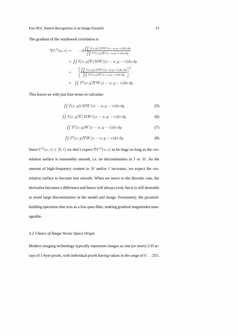
The gradient of the windowed correlation is

∇C2(u, v) = −2

∫∫

I(x,y)(MW )(x−u,y−v)dx dy∫∫

I2(x,y)W (x−u,y−v)dxdy

×∫∫

I(x, y)∇(MW )(x − u, y − v)dx dy

+

[∫∫

I(x,y)(MW )(x−u,y−v)dxdy∫∫

I2(x,y)W (x−u,y−v)dx dy

]2

×∫∫

I2(x, y)∇W (x − u, y − v)dx dy .

This leaves us with just four terms to calculate:

∫∫

I(x, y)(MW )(x − u, y − v)dx dy (5)

∫∫

I(x, y)∇(MW )(x − u, y − v)dx dy (6)

∫∫

I2(x, y)W (x − u, y − v)dx dy (7)

∫∫

I2(x, y)∇W (x − u, y − v)dx dy (8)

SinceC2(u, v) ∈ [0, 1] we don’t expect∇C2(u, v) to be huge so long as the cor-

relation surface is reasonably smooth,i.e. no discontinuities inI or M . As the

amount of high-frequency content inM and/orI increases, we expect the cor-

relation surface to become less smooth. When we move to the discrete case, the

derivative becomes a difference and hence will always exist, but it is still desirable

to avoid large discontinuities in the model and image. Fortunately, the pyramid-

building operation also acts as a low-pass filter, making gradient magnitudes man-

ageable.

3.2 Choice of Image Vector Space Origin

Modern imaging technology typically represents images as one (or more) 2-D ar-

rays of 1-byte pixels, with individual pixels having valuesin the range of0 . . . 255.


(a) (b) (c)

(d) (e)

Fig. 4 This figure shows the various representations required at each level of the pyra-

mid for gradient correlation search. The model is given in (a). The windowed version of

the model is shown in (b), with the windowing function shown in (c). The horizontal and

vertical components of the gradient are shown in (d) and (e).

While correlation values are in the range of−1 to 1, images represented solely by

non-negative integers will lead to purely non-negative correlation values.

An important example of this occurs when comparing the modelto a section

of the image which has uniform intensity. LetIconst = [a . . . a]T be a column

vector representing the uniform background. The correlation of a model with this

uniform background vector yields the following result:

C =M

TIconst

||M|| ||Iconst||.

Substituting the value ofIconst we get

C =

∑MhMw

i=1 mi

||M||√

MhMw

(9)

wheremi is the ith element ofM. We see that we get a correlation value that

depends only on the model. We also see that the choice of origin affects the value of

the correlation score. This is easily illustrated by remembering that the normalized


θ′

I′

M

I

θ

M′

Fig. 5 In this figure we see the effect of the choice of origin on the correlation score com-

puted for the two vectors. On the left we see two vectors whichcould easily result from

a positive-only imaging system, and the angle between them.On the right we see a much

larger angle achieved by choosing a different origin for thevector coordinates. In general,

for any two distinct vectors it is possible to choose an origin which makes the angle between

them any value, including 90 and 180 degrees.

correlation score is just the cosine of the angle between thetwo vectors, i.e.C =

cos θ whereθ is the angle betweenM andI.

In Figure 5 we see a graphic depiction of the effect of choice of the origin on

the correlation score. On the left we see a pair of vectors,M andI, which could

be a typical pair of image vectors. The angle between the two vectors isθ, which

is directly related to the correlation score (smaller angles correspond to higher

correlation scores, andvice versa). When all the vector components are positive,

then the resulting image vectors are limited to a subset of the image space. In the

2-D case shown here (think of the image vectors as having two pixels), the vectors

are limited to one quadrant of the vector space. In the 3-D case (think of the image


vectors as having three pixels), the vectors are limited to one octant of the vector

space. In general, the image vector will be confined to12N of the space, whereN is

the total number of pixels in the image. Since the models we are searching for will

routinely have hundreds and even thousands of pixels, we seethat the net result

of having only positive components in the vectors is that correlation scores will

tend to be high in most cases. On the right of Figure 5, the sametwo vectors are

depicted, but a new origin is being used. In this case the vectors are represented by

M′ andI′, and the angle between them isθ′. In this case the origin has been chosen

to makeθ′ = 90◦. In general, we can choose the origin to make the correlation

score anything we want (we can only makeC = 1 in the limiting case where the

origin tends to infinity).

Given an infinite number of choices for a new origin, which oneshould we

choose? One reasonable choice would be to choose an origin such that correlation

of the model with a uniform background leads to a score of0. Examining Eq. 9,

we see that subtracting the mean of the model vector components from the model

will cause

MwMh∑

i=1

m′

i = 0 .

Since a correlation score of+1 indicates a perfect match, and a score of−1 indi-

cates a perfect mismatch, then a score of0 for comparison with a featureless back-

ground seems reasonable. This method of subtracting the mean from the model

has been very successful in practice. It should also be notedthat subtracting the

mean from the model is the equivalent of removing any D.C. component from the

model image’s energy—thus only the energy related to model features is left.


A final issue to consider involves the effect of subtracting the model’s mean

from the image region being correlated with the model. Whileit seems reasonable

in practice to treat the image region in an identical fashionto the model, there are

some practical problems. If the mean is subtracted before the normalization is ap-

plied, then raw intensity of the model can affect the matching process. Since one

of the reasons we use NGC is for its robustness against changes in image intensity,

this is undesirable. In an image captured with pixel values in the range0 . . . 255,

pure multiplicative changes about the origin (0) are equivalent to a translation and

a multiplication when any other origin is chosen. It was observed in practice that

subtracting the same mean from both the model and the image region being com-

pared made the entire process very sensitive to changes in lighting. As a result, it is

proposed that the mean of the image region be subtracted instead. In this case we

are no longer doing pure NGC (since each vector has a different value subtracted

from it), but it works far better in practice. Again, one can think of this as having

removed the D.C. component from the image region.

3.3 Tuning the Pyramid

Up until now the only mention made ofK is that it is limited by the size of the

model. In many cases the details in the model may degrade too quickly for this

limit to be realistic. Take, for example, a model which consists of a checkerboard

pattern, with alternating pixels black and white. In this case even a 2-level pyramid

is too much, because the second level of the model pyramid will be a uniform

(featureless) grey region which will be useless for correlation.


Instead, the depth of the pyramid must be chosen according tothe characteris-

tics of the model itself. One method of doing this is to build the model pyramid one

level at a time, and as each new level is added estimate the worst-case correlation

score of the model with itself at that level.

By tuning the pyramidwe refer to the problem of deciding how many levels

to choose for a pyramid representation of a given model. Notethat this concept

is similar to the idea of finding an optimal template for matching, as described in

[12], although in our case we are searching for an optimal representation based on

a single exemplar, as opposed to combining multiple exemplar images into a tem-

plate. The more levels the pyramid has, the greater the savings in computation, but

building the pyramid with too many levels may render the model unrecognizable

to the NGC algorithm running at the top of the pyramid. The following discus-

sion on the effects of pyramid sampling gives a possible solution to the problem of

tuning the pyramid.

3.3.1 Issues Surrounding Sampling of the PyramidUsually a model is chosen

as a sub-image in a larger image. It is possible that we will then look for other

instances of that model in the same image, or we may wish to remember the model

and try and find it again later.

Consider, for example, that we have a model of size50×50 located at(96, 96)

in the image. The model pyramid will have 4 levels of size50 × 50, 25 × 25,

12 × 12 and6 × 6. If we look at the top-level of the model we will find an exact

replica of it in the top-level of the image pyramid (save integer division truncation

errors), since the location of the model is on an integral 8-pixel boundary, and our


4 level pyramid has a top-level where each pixel is represented by8× 8 = 64 pix-

els from the bottom-level. This guarantees that the same information is averaged

and combined in the exact same way while building both the image and model

pyramids. But what would happen if the model had been at(97, 97)? Then the

top-level representation of the target is not the same in theimage pyramid as in the

model pyramid. Since at(96, 96) the top-level instance will have a score of1, the

score when the model is at(97, 97) will generally be worse. For a two-level pyra-

mid we require the model to be on an even pixel boundary in order for the image

and model pyramid to match at the top. Therefore, for a randomly placed model

there is one chance in four that it will land perfectly. For a three-level pyramid, the

model must land on an even boundary of 4 pixels, giving one chance in sixteen

of perfect alignment. There is one chance in 64 for perfect alignment in a 4-level

pyramid.

It should be noted that perfect alignment is not required in order to be able to

find the target at the top level of the pyramid. How well an imperfectly aligned

model will match at the top of the pyramid is dependent on the features of the

model.

3.3.2 Tuning the Pyramid using Worst-Case AnalysisAs discussed earlier, the

representation of a target at the top of the pyramid may be better or worse depend-

ing on its location in the image. This suggests a possible method for tuning the

pyramid.

The first step is to set an upper limit on the number of levels inthe pyramid.

Obviously correlation is meaningless with only one pixel atthe top level of the


pyramid, so we can choose a minimum size for the model at the top-level. For the

current implementation of the search tool this minimum sizehas been chosen to

be4 × 4. This means that the maximum number of levels in the pyramid will be

chosen so that the model has a minimum dimension between4 and7 (a minimum

dimension of8 could be reduced to4 by adding another level to the pyramid).

Depending on the features of the model it may be possible to successfully search

at this maximum pyramid depth.

The second step is to consider the worst-case score of the model at different

pyramid depths. The worst-case will be be due to the effects of pyramid sampling

as discussed in Section 3.3.1. In order to determine the worst-case score of a model

in a K-level pyramid, we build the model pyramid toK levels, and then build a

test pyramid based on the model but with offsets(x, y) where bothx andy are in

the range0 . . . 2k−1−1. Therefore we end up considering22(k−1) different offsets

at each pyramid levelk. Of course, the offset(0, 0) is expected to have a score of

1.

It is important to note that this worst-case analysis is onlyan estimate of the

worst score of the model at the top of the pyramid, since in a real search situation

that score will depend on image content outside the target for which we have no

a priori knowledge. As we consider different offsets, the size of thetest pyramid

(really just a shifted version of the model) can be as much as one-pixel smaller

than the model in each level. If we consider the most extreme case, we compare a

4 × 4 model to a3 × 3 test-image. In this case our estimate involves comparing

56.25% of the model with a shifted version of itself.


The third step is to perform this worst-case analysis for pyramids from level

2 up to and including the maximum possible number of levels, and choosing the

maximum pyramid depth that still yields an acceptable worst-case score.

A number of pathological targets can be imagined in order to test this scheme.

Consider black & white checkerboard patterns where each cell of 2 white and 2

black squares takes on the following dimensions:2× 2, 4× 4, 8× 8 and16× 16.

The first pattern can only be searched with a 1-level pyramid,since the2 × 2

receptive field used to go to the next level will blur the checks into a featureless

pattern of grey. The second pattern could be searched with a 2-level pyramid if we

were confident that the target would always align perfectly on a 2-pixel boundary.

However, since this is not guaranteed, we will likely end up with a featureless grey

again (corresponding to an offset of(1, 1)), so we must restrict ourselves to a 1-

level pyramid. The next two patterns (for similar reasons) may be searched reliably

with a 2-level pyramid, but no more.

To recap the worst-case analysis algorithm, we perform the following steps:

1. Based on the size of the model in the original image, determine the maximum

depth (number of levels) of the pyramid that will make the top-level repre-

sentation of the model larger than a pre-set minimum size (inour case4 × 4

pixels). Call this depthKmax.

2. Build the model pyramid to this depth.

3. For each pyramid of depthk in the range of2 . . .Kmax perform a worst-case

analysis of the test-image representation of the model at level k. This is done

by building a test-image pyramid based on the original model, but offset by


Fig. 6 The correlation surface from the top level of the pyramid is shown. Two strong

peaks, representing the location of the two instances of themodel, are evident. These peaks

provide coarse location estimates, which are refined as the algorithm descends through the

pyramid.

(x, y) where each ofx andy takes on values in the range0 . . . 2K−1 − 1. For

each image, compute the correlation score between thekth level representation

of the image and the model.

4. Choose the number of levels in the pyramid to be the largestvalue ofk for

which the worst-case correlation score between model and test-image is above

some pre-set threshold (currently we are using 0.1 for this threshold).

Intuitively this method is quite appealing, in that it mimics the actual search

process when deciding how to tune the pyramid. Unfortunately, it may well be that

always catering to the worst-case is unduly pessimistic. Variations on the method,

in which the average or median of returned scores is used instead of just the worst-

case itself, may prove useful.


The worst-case score found at the top-level of the model pyramid can be used

to determine what threshold to use in accepting candidates at the top-level cor-

relation. If, for example, the worst-case score is 0.7, and the correlation accept

threshold entered by the user is 0.8, then the threshold for accepting candidates at

the top-level could be set to0.56 = 0.7×0.8. In this way candidates that are imper-

fect matches in the original image, and whose scores degradein coarser pyramid

levels, can still be found by the algorithm.

4 Implementation, Experiments & Results

The algorithm has been implemented in C++, and compiled on a Windows-based

PC using Visual C++ V6.0. The core algorithms are not Windowsspecific and can

be (and have been) re-compiled on other platforms, including Linux. No special

effort has been made to optimize the run-time efficiency of the code. The results

that follow are from an AMD Athlon Thunderbird 750 MHz systemwith 256 MB

of RAM. In all cases the accept threshold is set to 0.75, representing a correlation

score of0.866 =√

0.75. Except where otherwise noted, the algorithm has been

given the expected number of targets in advance. Results aregiven for search time

vs. number and size of targets and false positive/negative results are also given.

Finally, the algorithm is tested for sensitivity to slight variations in scale and rota-

tion of the targets. Results are also shown for real-world images where the target

undergoes mild perspective distortion. Finally, the performance of the algorithm

with respect to sub-pixel localization is presented.


4.1 Comparison with Full Correlation

To demonstrate the speedup of our method over full correlation (no pyramid struc-

ture or gradient search), the two were compared for a typicalimage search. The

search shown in Figure 16(a) was conducted on the full-sizedimage,2272 ×

1704pixels , using a target260 × 96 pixels in size. Our method required 0.547

seconds2 The same search performed using full correlation yielded identical re-

sults, but took 450.922 seconds to complete. Both the searchand target images

were resized by 50%, and the experiment repeated. This time our method took

0.312 seconds, while full correlation required 29.375 seconds. By way of con-

firmation, note that450.922/16 ≈ 28, suggesting that the full correlation result

scales roughly according to the inverse of the product of thesearch and target pixel

counts, as expected. This simple experiment demonstrates the potential speedup

using our technique.

4.2 Top-Level Correlation Scores

As an example of how candidate scores can degrade in higher (coarser) levels of

the pyramid, Table 1 shows the squared-correlation scores at the lowest and highest

pyramid levels for the target instances shown in Figure 2. Instance 1, which also

serves as the model, has perfect scores at both levels as we might suspect. However,

instance 2 has a score of 0.950 at the lowest level (the original search image), but

a poorer score of 0.796 two levels higher in the pyramid.

2 This test was performed using a VMware virtual machine running Windows XP, on a

host machine running Ubuntu Linux on a 2.16 GHz Centrino Duo processor.


Instance Location Score (level 0) Score (level 2)

1 (322,304) 1.000 1.000

(model)

2 (318, 95) 0.950 0.796

Table 1 Squared Correlation Scores for Model in Figure 2

4.3 Search Timevs.Number of Target Instances

Results are shown in Figure 7 for the effect of number of target instances on the

search time. In the lower trace we see that as the number of instances increases, the

search time increases in a roughly linear fashion. This is tobe expected. The search

time can be thought of as the overhead of building the pyramidrepresentation of

the search image, plus the time to evaluate individual candidates. If the algorithm

has already found the requested number of target instances,it can terminate early.

If it does not have an upper bound, then it will continue to evaluate candidates

until no more suitable candidates are found in the top-levelcorrelation. This may

prolong the search if the image contains distractor patterns that are sufficiently

similar to the target. This extra time may be reduced by setting a higher accept

threshold, which in turn causes less candidates to be considered at the top-level

correlation. The upper trace in the figure is an example of roughly constant search

time in the case of not knowing how many instances to expect. In this case, random

distractor blobs were used to test the algorithm’s ability to find the correct target.

When distractors are not present, the search time in both cases is very similar.


0 5 10 150

0.05

0.1

0.15

0.2

0.25

0.3

0.35

Number of Targets

Sea

rch

Tim

e (s

econ

d)

Figure: Search Time vs number of targets

Not Knowing MaxHit

Knowing MaxHit

Fig. 7 This figure shows the increase in search time as more target instances are found. In

the upper trace the algorithm does not know the number of targets to expect in advance,

and has to consider distractor blobs in the image. In the lower trace it knows the expected

number of targets, illustrating the advantage of giving thealgorithm an upper bound on the

expected number of targets.

It should be noted that in the case where multiple targets areto be searched for

in the same image, the overhead of constructing the image pyramid will only be

required once, leading to more efficient searches.

4.4 Search Timevs.Size of Model

Using NGC in a non-pyramid framework we would expect search times to increase

as the size of the model increased. As the model size increases, we reach a point

where another level may be added to the model pyramid (depending on the results

of the worst-case analysis), resulting in asmallermodel at the top of the pyramid,

as well as a smaller search image at the top of the pyramid. There is extra overhead


to build one more level in the search pyramid, but this gets smaller for each level

of the pyramid by a factor of 4, and the savings in correlationcomputations more

than offsets this. It should also be noted that rectangular models use the minimum

dimension to limit pyramid size, so this further complicates the relation between

size and search time.

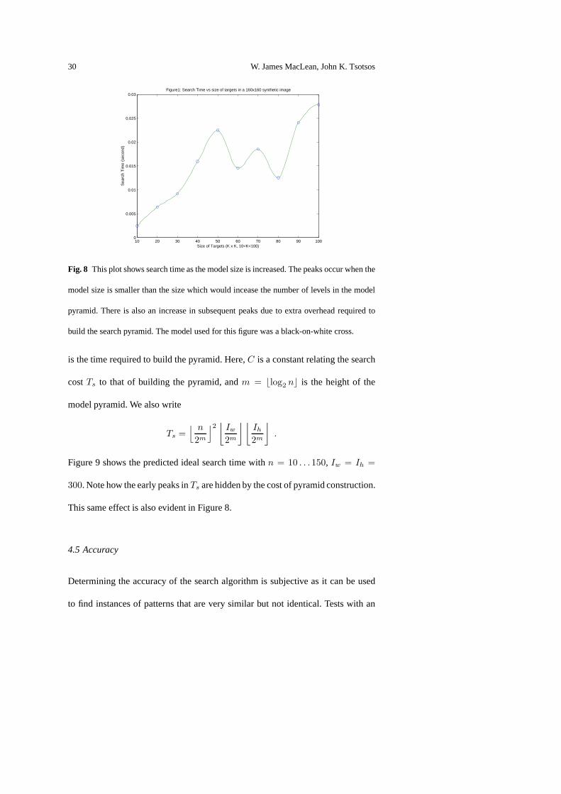
In Figure 8 we see the results of varying model size on search times with the

number of target instances held fixed, and the size of the image being searched

held fixed. The results shown are from a set of real images captured using a cam-

era at varying distances from the target and distractors. Inthe graph we see that

search times gradually increase as the target is increased in size to 50 pixels, then

they suddenly decrease, only to incease to a new maximum at 70pixels, and fi-

nally another increase to a new maximum at greater than 100 pixels. The point at

which new pyramid levels are built is further controlled by the worst-case analy-

sis, so changes may not occur exactly at sizes that are an evenpower of 2. The line

joining the data is a smooth interpolation. For small model sizes we may not see

the same pattern of increases and decreases as the algorithmplaces a hard-limit on

the smallest allowed model at the top of the model pyramid, thus preventing the

pyramid from attaining its full depth in some cases.

It is instructive to develop a simple model explaining the search-time as a func-

tion of model size. Assume we have a model of sizen × n in an image of size

Iw × Ih. The total search time (up to the end of the top level correlation) can be

written asT = Ts + Tp where

Tp = CIwIh

(

1 +1

22+

1

24+ · · · + 1

22(m−1)

)


10 20 30 40 50 60 70 80 90 1000

0.005

0.01

0.015

0.02

0.025

0.03

Size of Targets (K x K, 10<K<100)

Sea

rch

Tim

e (s

econ

d)

Figure1: Search Time vs size of targets in a 160x160 synthetic image

Fig. 8 This plot shows search time as the model size is increased. The peaks occur when the

model size is smaller than the size which would incease the number of levels in the model

pyramid. There is also an increase in subsequent peaks due toextra overhead required to

build the search pyramid. The model used for this figure was a black-on-white cross.

is the time required to build the pyramid. Here,C is a constant relating the search

costTs to that of building the pyramid, andm = ⌊log2 n⌋ is the height of the

model pyramid. We also write

Ts =⌊ n

2m

⌋2⌊

Iw

2m

⌋⌊

Ih

2m

⌋

.

Figure 9 shows the predicted ideal search time withn = 10 . . .150, Iw = Ih =

300. Note how the early peaks inTs are hidden by the cost of pyramid construction.

This same effect is also evident in Figure 8.

4.5 Accuracy

Determining the accuracy of the search algorithm is subjective as it can be used

to find instances of patterns that are very similar but not identical. Tests with an


0 50 100 1500.033

0.0332

0.0334

0.0336

0.0338

0.034

0.0342

Size of Model (pixels)

Rel

ativ

e S

earc

h T

ime

Idealized Search Time vs. Model Size

Fig. 9 Idealized search times generated by search complexity model. Notice the similarity

to Figure 8. As the relative cost of building the pyramid increases, early peaks in the plot

are smoothed out.

accept threshold of 0.95 have yielded a false positive rate of less than0.1%. As the

threshold is lowered, the algorithm will match instances with increasing variabil-

ity. In the extreme, one could imagine matching anything with an accept thresh-

old of 0. Even an accept threshold of 0.75 may miss target instances which we

would consider good, as is shown in Figure 10 (a). In this case, a change in the

background surrounding the instance, plus different shading in the middle of the

target, is enough to cause its rejection at this threshold level. The important thing

to recognize here is that correlation scores do not always coincide with perceptual

judgements. Occlusion and shading are also known to adversely affect correlation

matching, and are not explicitly examined in this section.

False negative rates are affected not only by accept threshold, but also by the

maximum target instance parameter if it is specified. Targetinstances may also be


(a)

(b)

Fig. 10 Two images in which searches have taken place. In (a) we have an example of

a false negative (white box), but the missed target instanceis noticeably different due to

background shading. In (b) we have no false results despite relative similarity of all objects

in terms of size and intensity levels.

rejected if they cross the borders of the image, as the current implementation only

looks for instances wholly contained within the search image. In summary, almost


all false results occur when the target instance is not identical, or close to identical,

to the model.

4.6 Sensitivity to Small Scale and Orientation Changes

Even though normalized correlation is not designed to accomodate changes in

scale and orientation, tests show that in some cases it may doquite well. In Fig-

ure 11 correlation scores are shown for small changes in scale and orientation of

the target instance.

These results suggest mechanisms by which scale and orientation invariance

might be built into the algorithm. In the case of scale, the pyramid would easily

allow for searching over different scales separated by a factor of 2. If we create a

number of re-scaled versions of the model to be searched at each pyramid level (in

this case each about 1.2 times larger/smaller than the previous one), then the algo-

rithm could be used to search over the range of1/√

2 to√

2. Anything larger or

smaller could be searched in the next scale. A schedule for searching at the differ-

ent pyramid levels can be devised, and the number of additional models required

at each level can be determined via worst-case analysis. In the case of rotation, a

method similar to that of [26] can be used to determine the number of additional

target templates required to search for rotated versions ofa target.

4.7 Subpixel Localization

In identifying an object in an image using NGC, it may be the case that the object as

found will not align with the pixel grid in the same way as the model (or template)


−15 −10 −5 0 5 10 150.75

0.8

0.85

0.9

0.95

1

Scale (percent)

Sco

re

Figure1: the correlation score of circles vs Scale

(a)

−15 −10 −5 0 5 10 150.4

0.5

0.6

0.7

0.8

0.9

1

Angle rotated (degree)

Sco

re

Figure1: the correlation score vs degree of rotation

(b)

Fig. 11 This figure shows the effect of slight changes in both (a) scale and (b) orientation

on the correlation scores. Scale was varied by±10% resulting in correlation scores from 0.8

to 1.0. The target used was a black ellipse on a white background. Orientation was varied

by ±14◦ resulting in squared-correlation scores from 0.418 to 1.0.The target used was a

black cross on a white background. The use of simple, high-contrast targets is intended to

isolate the method’s ability to recognize shapes.


did. In this event, our estimate for the location of the object is expected to lie

betweenpixels. Since NGC only allows us to compute the correlation at integral

pixel locations, some method of determining the sub-pixel location is needed. One

such method is interpolation using abi-quadraticsurface as described in [20]. In

this section we give performance results for this method.

Two sets of tests were done. The first set involves a series of 10 images pro-

duced by synthetic means. Software was devised to simulate atarget moving in

the horizontal direction at 0.1 pixels/frame. The main advantage to using synthetic

images is that ground truth is known for the target location.However, the synthetic

data ignore the possibility of effects introduced by imperfections in the imaging

system.

The synthetic images were created by creating a target at a higher resolution

than the original image, and then averaging over the required subset of pixels in

order to determine the target’s representation in the low-resolution image.

The second set of images involve a printed circuit board, with the board being

shifted left by roughly1/20 of a pixel in each subsequent image using a camera

mounted on a mechanical X-Y translation stage. No absolute orientation between

the camera and the stage is sought—the important thing is that the base of the

stage is stationary with respect to the scene, so the changesbetween images is

solely related to the controlled movement of the camera. Themethod of fixing the

camera to the stage rougly aligns the camera’s horizontal and vertical directions

to those used by the stage itself. There are 20 images in the sequence. This image


sequence permits meaningful testing of the subpixel localization algorithm on real

images.

In both sets of images, the model is defined in the first image, where its location

(by definition) lies exactly on an integer pixel boundary. Ineach image sequence

the target is assumed to shift by roughly equal amounts from one image to the

next.3 As a model is tracked, therefore, the subpixel estimate for its location should

form a straight line with respect to the frame number.

For analysis of the images, four image regions were selectedas models, and

each region was searched in each image in order to obtain an estimate of its loca-

tion using subpixel localization.

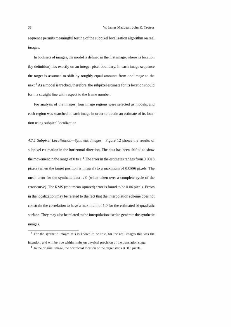
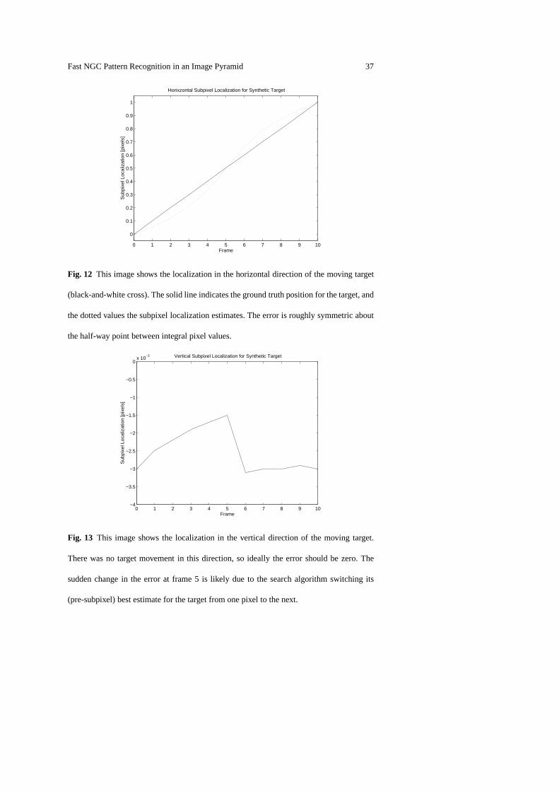
4.7.1 Subpixel Localization—Synthetic ImagesFigure 12 shows the results of

subpixel estimation in the horizontal direction. The data has been shifted to show

the movement in the range of0 to1.4 The error in the estimates ranges from0.0018

pixels (when the target position is integral) to a maximum of0.0886 pixels. The

mean error for the synthetic data is0 (when taken over a complete cycle of the

error curve). The RMS (root mean squared) error is found to be0.06 pixels. Errors

in the localization may be related to the fact that the interpolation scheme does not

constrain the correlation to have a maximum of 1.0 for the estimated bi-quadratic

surface. They may also be related to the interpolation used to generate the synthetic

images.

3 For the synthetic images this is known to be true, for the realimages this was the

intention, and will be true within limits on physical precision of the translation stage.4 In the original image, the horizontal location of the targetstarts at 318 pixels.


0 1 2 3 4 5 6 7 8 9 10

0

0.1

0.2

0.3

0.4

0.5

0.6

0.7

0.8

0.9

1

Frame

Sub

pixe

l Loc

aliz

atio

n [p

ixel

s]

Horixzontal Subpixel Localization for Synthetic Target

Fig. 12 This image shows the localization in the horizontal direction of the moving target

(black-and-white cross). The solid line indicates the ground truth position for the target, and

the dotted values the subpixel localization estimates. Theerror is roughly symmetric about

the half-way point between integral pixel values.

0 1 2 3 4 5 6 7 8 9 10−4

−3.5

−3

−2.5

−2

−1.5

−1

−0.5

0x 10

−3

Frame

Sub

pixe

l Loc

aliz

atio

n [p

ixel

s]

Vertical Subpixel Localization for Synthetic Target

Fig. 13 This image shows the localization in the vertical directionof the moving target.

There was no target movement in this direction, so ideally the error should be zero. The

sudden change in the error at frame 5 is likely due to the search algorithm switching its

(pre-subpixel) best estimate for the target from one pixel to the next.


Figure 13 shows the vertical error. Since the target was not moving vertically,

we expect this error to be roughly constant, and ideally0. The mean error was

−0.0025 pixels, and the RMS error was0.0026 pixels. We see a sharp change in

the error around frame 5. To understand this, recall that thesubpixel localization

algorithm starts from9 correlation values centred on the best integral estimate of

the target position. At frame 5 we are half-way between pixels, and we should

expect the best integral estimate to switch from one pixel tothe next at this point.

4.7.2 Subpixel Localization—Structured ImagesThe data derived from the four

image regions tracked through a real image sequence, of a printed circuit board,

was analyzed in an attempt to gauge the performance of the subpixel localization

algorithm. First, since it was assumed that all movement in the image sequence

was purely in the horizontal direction, any changes in the vertical ordinate of the

estimates should represent noise. In Figure 14 we see a plot of they-ordinates from

the four data sets. Each data set has been adjusted to start at0 so that they could

be plotted together. The mean error,y is calculated as

y =1

N

N∑

i=1

yi

whereyi are the adjustedy data. The value obtained is 0.003 pixels. Since each

target is defined in the first image in the sequence, we expect the error to have

zero average over the image sequence, assuming the translation stage is properly

aligned with the camera. The root-mean-square error, defined as

σy =

√

√

√

√

1

N

N∑

i=1

(yi − y)2


0 2 4 6 8 10 12 14 16 18 20−0.025

−0.02

−0.015

−0.01

−0.005

0

0.005

0.01

0.015

0.02

0.025

Frame

Sub

pixe

l Loc

atio

n [p

ixel

s]

Subpixel Measurement: IMG01−20 (Vertical)

Fig. 14 This figure shows the vertical ordinates of the subpixel localization estimates over

the entire image sequence. The estimate shown for Frame 0 is that obtained with subpixel

localization turned off. Each data set has been adjusted so that the first element is zero. Data

sets 1–4 are represented by *, +, X and o, respectively.

was measured to be 0.009 pixels. As expected from looking at Figure 14, this error

is quite small.

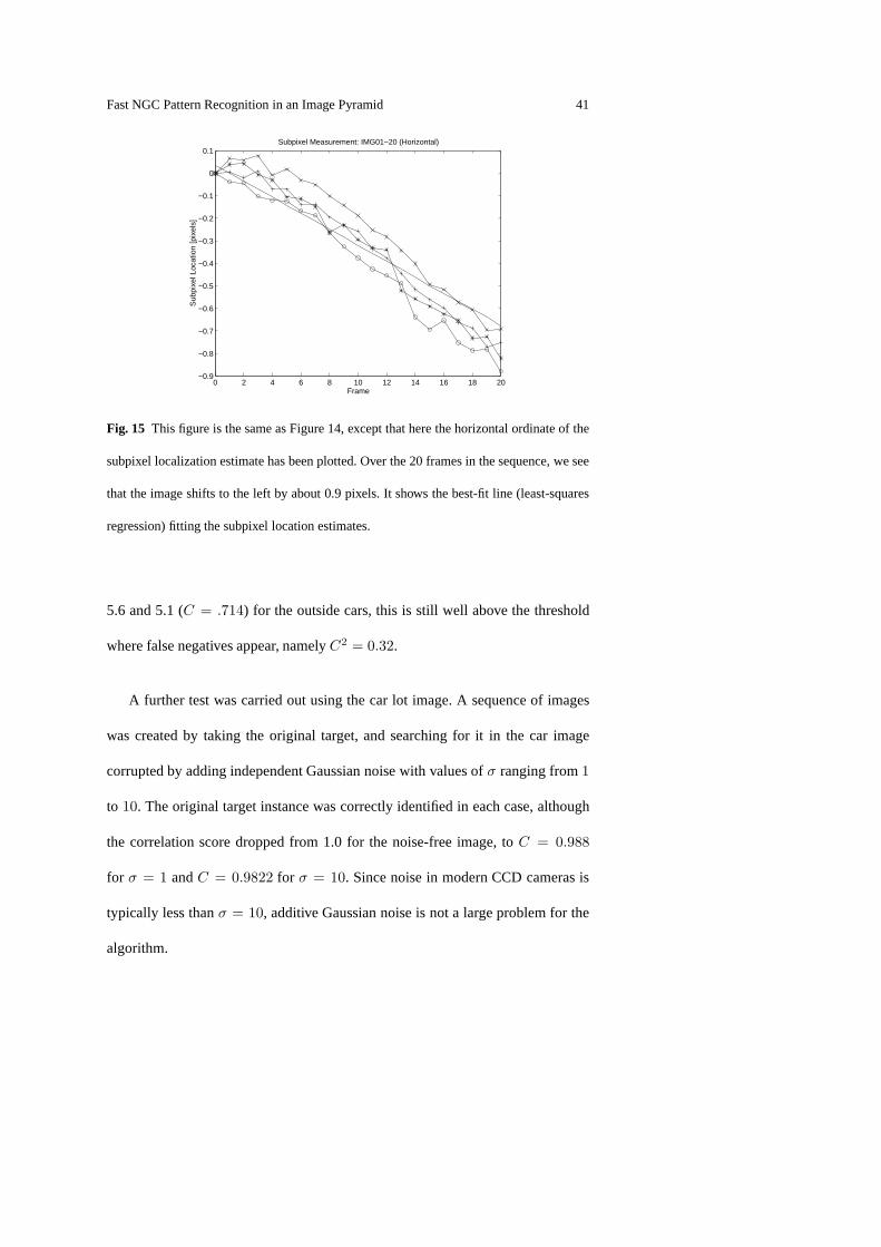
Unlike the vertical ordinates, the horizontal (x) ordinate estimates are expected

to change. Since the image moves approximately one pixel to the left over 20

frames, we would expect a change of about−0.05 pixels/frame. As seen from the

plot in Figure 15, the slope of these lines is indeed negative, and a quick estimate

shows it to be approximately the right size. In order to get a more accurate measure

of the error, a linear least-squares regression was performed on the data.

Figure 15 shows the best-fit line from the regression done assuming the line

had zero intercept. The line has a slope of−0.0356 pixels/frame. The mean error


in the data with respect to the regression line is−0.0034 pixels, and the RMS error

is 0.09 pixels.

Another meaningful test is to pick out multiple regions in animage as targets,

and then search for them in the same image. In this case the exact target loca-

tion is known, and it is known to be an exact integral value. The subpixel location

estimates will not return exactly integral values and are expected to be in error—

the question is “how much?”. In a set of data collected using this approach (15

regions), the horizontal location error was found to have a mean error of0.0676

pixels and an RMS error of0.1264 pixels in the horizontal direction. The corre-

sponding values for the vertical direction are0.0094 and0.0305 pixels, respec-

tively. It must be mentioned that several of the targets werestructure deficient,i.e.

they were composed of lines almost exclusively in one direction, in this case hori-

zontal, leading to some large error values in the horizontalestimate. The mean and

RMS error values would doubtlessly be lower if these sampleswere omitted.

4.8 Results From Unstructured Scenes

In this section, real-life examples of searching for targets are presented. In Fig-

ure 16 two examples are shown of images acquired at a car dealership. In Fig-

ure 16(a) the technique is applied to find matches for the front end of the middle

car. Due to perspective distortion, the front-end details of the cars to both the right

and left of centre are noticeably different from those of thecentre car. While the

squared correlation scores drop to 7.0 and 7.5 for the immediate neighbours, and


0 2 4 6 8 10 12 14 16 18 20−0.9

−0.8

−0.7

−0.6

−0.5

−0.4

−0.3

−0.2

−0.1

0

0.1

Frame

Sub

pixe

l Loc

atio

n [p

ixel

s]

Subpixel Measurement: IMG01−20 (Horizontal)

Fig. 15 This figure is the same as Figure 14, except that here the horizontal ordinate of the

subpixel localization estimate has been plotted. Over the 20 frames in the sequence, we see

that the image shifts to the left by about 0.9 pixels. It showsthe best-fit line (least-squares

regression) fitting the subpixel location estimates.

5.6 and 5.1 (C = .714) for the outside cars, this is still well above the threshold

where false negatives appear, namelyC2 = 0.32.

A further test was carried out using the car lot image. A sequence of images

was created by taking the original target, and searching forit in the car image

corrupted by adding independent Gaussian noise with valuesof σ ranging from1

to 10. The original target instance was correctly identified in each case, although

the correlation score dropped from 1.0 for the noise-free image, toC = 0.988

for σ = 1 andC = 0.9822 for σ = 10. Since noise in modern CCD cameras is

typically less thanσ = 10, additive Gaussian noise is not a large problem for the

algorithm.


In Figure 17 we show results for images similar to those used in [4]. The target

(Figure 17(b)) was obtained by scanning Waldo’s face from the instruction page

at the front of “Where’s Waldo? The Wonder Book” [8]. This image was rescaled

by eye to approximately match the size it appears elsewhere in the book using the

GIMP (GNU Image Manipulation Program). The target image was21× 40 pixels

in size. The search was performed on a grey-scale version of the images, and was

successful, as shown in the subset of the search region reproduced in Figure 17(a).

The squared correlation score was0.37 (C = 0.608), which is good considering

the slight changes in the details of Waldo’s face and the dot-screening process used

to print the book (we do not expect the dots on the target to align exactly with those

in the recovered instance). Finding Waldo without colour ishelpful, since in at

least one Waldo image all other characters are dressed just like Waldo, meaning a

method such as [4] that only uses colour information will be confounded. However,

if colour information is helpful, our method can use colour correlation instead of

grey-scale to take advantage of colour as well as image structure.

4.9 Timing Comparison with Feature Detectors

In order to better describe the performance of our method, this section provides

some timing comparisons with a number of current feature detectors, including

SIFT and some affine-invariant techniques.

In Table 2 we see a timing comparison of a number of feature detectors. The

first two entries in the table give different reports of SIFT detectors, and both show

times of 0.3 seconds for small images [34] and medium size images [19], even


(a)

(b)

Fig. 16 Two examples from unstructured images are shown. In (a) the target was chosen

from the centre car, and squared correlation scores range from 0.51 for the car on the ex-

treme left to 1.0 for the centre car as expected. This exampleshows performance in the

presence of a moderate amount of perspective distortion. In(b) the target was chosen from

the left wheel, and the right wheel is recovered, despite thepresence of some rotation, as

well as differences in the brake and pavement details.

though the latter is using a much faster processor than the first (or than the pro-

cessors used in this paper). The next four entries are found in [25], which contains

a comparison of a number of affine-invariant feature detectors. Both the Harris-

Affine and the Hessian-Affine attempt to localize the feature, and compute an el-

lipsoidal region describing its scale and orientation (as opposed to Mikolajczyk &

Schmid’s affine-invariant detector, which iteratively warps the image around the

feature point to create a circular region). IBR (intensity extrema-based region de-

tector) explores regions around intensity extrema, using an affine-invariant func-


(a)

(b)

Fig. 17 In (a) we see an example of “Where’s Waldo?”. Our algorithm easily finds Waldo

in the lower-left corner. The target, shown enlarged in (b),was taken from the instructions

at the front of “Where’s Waldo? The Wonder Book” [8], while the search region (a subset of

which is shown in (a)), was scanned from later in the book (“The Corridors of Time” page).

The match score wasC2= 0.37, but given the slight differences in Waldo’s appearance and

the dot-screening process used to print the book, this is quite good for a correlation-based

search technique. [Permission to reproduce these images courtesy Mike Gornall, Egerton,

Kent, England.]


Algorithm Time Image Size Hardware Reference

SIFT 0.3–0.4 S 340 × 240 Pentium III 700 MHz [34]

SIFT 0.3 S 640 × 314 Pentium IV 2 GHz [19]

Harris-Affine 1.43 S 800 × 640 Pentium IV 2 GHz [25]

Hessian-Affine 2.73 S

MSER 0.66 S

IBR 10.82 S

Table 2 This chart shows a comparison of the running time of several popular feature de-

tection algorithms.

tion of intensity evaluated along radial lines, and the lociof the extremums of

this function are approximated by an ellipse, whose scale and orientation define

the feature region. MSER (maximally-stable extremal regions) identifies regions

based on their intensity with respect to a threshold, and finds regions that are stable

over a number of threshold levels [1]. Note that feature computation times for the

non-SIFT features does not include grouping or matching against known objects.

We see that even SIFT, although it is closest in terms of computation time to our

method, is still somewhat slower that our technique.

The MSER detector is the only other detector whose speed comes close to

SIFT, albeit for larger images and running on a faster processor than used in this

paper. While these detectors have similarity/affine invariance that our method does

not provide, our method typically runs faster, and may proveuseful in situations

where only translation invariance is required. One such example is automated vi-


sual inspection tasks where the part under inspection has a known orientation and

distance with respect to the camera.

5 Discussion

In Section 4 we see that our method has good performance in finding targets even

in the presence of small amounts of rotation and scale change.

The algorithm is also very fast even on modest hardware, making it attrac-

tive for machine vision applications in industry. Only two other methods, those of

Lowe [18] and Schiele & Pentland [32] cite similar speeds. Since the latter system

is designed for detection, and not localization, we will notconsider it further. In

comparing our algorithm to that of [18], we note that it is more complex to imple-

ment than our algorithm, and that its method of finding features through analysis

of feature stability across scale makes it less suitable forsearching for small tar-

gets such as that shown in Figure 17(b). Further, we expect our method to better

detect subtle differences in target instances as it does a pixel-by-pixel compari-

son. As mentioned in Section 2, Lowe’s algorithm uses features that may fail to

match under global illumination changes, causing the search to fail. While it may

be possible to correct this using features such as those in [3], this would incur

considerable computational expense and hinder the speed ofthe algorithm. Our

algorithm, being based on NGC, is robust over a wide range of global illumination

changes. In defense of SIFT, it has rotation and scale invariance while our method

does not. This is a great advantage. Finally, our algorithm is applicable to tech-

niques such as those cited by [37,26], since these techniques perform matching by


correlating candidate images against a set of templates determined by PCA. It is

possible that a combination of our method with that of [26] would allow efficient

search for rotated targets. Further, searching for slightly re-scaled versions of the

target across pyramid levels (as described in Section 4.6) would allow our method

to find targets across a range of scales.

The speed of the search is largely dependant on the number of levels in the

target pyramid. In the case of the checkerboard pattern where each square is one

pixel, we expect performance to be very slow since only one level exists in the

pyramid, and the algorithm is reduced to that of ordinary NGC. Nonetheless, it

will still work. In practice such degenerate target patterns are the exception and

not the rule, and the system typically works with a 3- or 4-level target pyramid,

resulting in substantially faster operation.

The choice of the accept threshold will have a strong effect on the results. As

this threshold is reduced we would expect to find a larger number of false positives.

Of course, it is somewhat subjective as to what constitutes amatch in the first place,

and this will vary depending on the task for which the search is used. It must be

remembered that lowering the accept threshold also leads toa larger number of

candidate matches at the top level of the pyramid, and this inturn will generally

lengthen the search time.

6 Conclusion

This paper describes a novel approach to pattern matching based on normalized

correlation matching in a pyramid image representation. Three main contributions


are made: (1) incorporation of NGC search into a multi-scaleimage representa-

tion, (2) use of an estimate of the correlation gradient to perform steepest descent

search at each level of the pyramid, and (3) a method for choosing the appropri-

ate pyramid depth of the model using a worst-case analysis. The result is a fast

and robust method for localising target instances within images. Further, since it

is based on correlation search, the technique is simple and easily combined with

PCA techniques for target matching.

The algorithm is limited in that it does not attempt to deal with variable size or

orientation of target instances, although it is shown to be robust to small variations

in either parameter. The level of robustness is dependent onthe actual pattern to

be searched for, but this can be included in the worst-case analysis. The technique

is also sensitive to image warping due to out-of-plane rotations, although again a

small amount can be tolerated. A procedure for allowing size-invariant searches is

outlined. Future work includes further investigation of size, and even orientation,

invariance in the search framework.

Possible applications for this algorithm include machine inspection of printed

circuit boards, finding parts in an industrial setting, and identifying trademarks and

copyright material on the Internet. In this latter vein the authors have built a search

engine that follows HTML links, download images and searches them, and records

the URLs of any matches found. Through judicious choice of the accept threshold,

unauthorized modifications to trademarks were also found.


Aknowledgements

The authors would like to thank Fernando Nuflo and Fang Liu fortheir contribu-

tions to the testing of the algorithm.

References

1. A. Baumberg. Reliable feature matching across widely separated views. InIEEE

Conference on Computer Vision & Pattern Recognition, pages 774–781, 2000.

2. P. Burt. Attention mechanisms for vision in a dynamic world. In Proceedings of the

International Conference on Pattern Recognition, pages 977–987, 1988.

3. Gustavo Carneiro and Allan D. Jepson. Multi-scale phase-based local features. InPro-

ceedings of the IEEE Computer Society Conference on Computer Vision and Pattern

Recognition, volume 1, pages 736–743, Madison, WI, June 2003.

4. Francois Ennesser and Gerard Medioni. Finding Waldo, or focus of attention using

local colour information.IEEE Transactions on Pattern Analysis and Machine Intelli-

gence, 17(8):805–809, August 1995.

5. Rafael C. Gonzalez and Paul Wintz.Digital Image Processing. Addison-Wesley Pub-

lishing Company, Reading, Massachusetts, 2nd edition, 1987.

6. Ardeshir Goshtasby. Template matching in rotated images. IEEE Transactions on

Pattern Analysis and Machine Intelligence, PAMI-7(3):338–344, May 1985.

7. Michael A. Greenspan. Geometric probing of dense range data. IEEE Trans. Pattern

Anal. Mach. Intell., 24(4):495–508, 2002.

8. Martin Handford.Where’s Waldo? The Wonder Book. Candlewick Press, 1997.

9. Chris Harris and Mike Stephens. A combined corner and edgedetector. InProceedings

Fourth Alvey Vision Conference, pages 147–151, Manchester, United Kingdom, 1988.


10. Berthold Klaus Paul Horn.Robot vision. The MIT Press, Cambridge, Massachusetts,

1986.

11. M. K. Hu. Visual pattern recognition by moment invariants. IRE Trans. Information

Theory, IT-8:179–187, 1962.

12. Y. S. Huang, C. C. Chiang, J. W. Shieh, and Eric Grimson. Prototype optimization for

nearest neighbour classification.Pattern Recognition, 35:1237–1245, 2002.

13. Anil K. Jain and Aditya Vailaya. Shape-based retrieval:A case study with trademark

image databases.Pattern Recognition, 31(9):1369–1390, 1998.

14. Jean-Michel Jolion and Azriel Rosenfeld.A pyramid framework for early vision.

Kluwer Academic Publishers, P.O. Box 17, 3300 AA Dordrecht,The Netherlands,

1994. ISBN: 0-7923-9402-X.

15. Yong-Sung Kim and Whoi-Yul Kim. Content-based trademark retrieval system using

visually salient feature. In1997 Conference on Computer Vision and Pattern Recogni-

tion, pages 307–312, Peurto Rico, June 1997.

16. Arun D. Kulkarni.Artificial Neural Networks for Image Understanding. Van Nostrand

Reinhold, New York, 1994. ISBN 0-442-00921-6; LofC QA76.87.K84 1993.

17. Tony Lindeberg.Scale-space theory in computer vision. Kluwer Academic Publishers,

P.O. Box 17, 3300 AA Dordrecht, The Netherlands, 1994. ISBN:0-7923-9418-6.

18. David G. Lowe. Object recognition from local scale-invariant features. InProceed-

ings of the Seventh International Conference on Computer Vision, pages 1150–1157,

Kerkyra, Greece, 1999.

19. David G. Lowe. Distinctive image features from scale-invariant keypoints.Interna-

tional Journal of Computer Vision, 60:90–110, 2004.

20. W. James MacLean and John K. Tsotsos. Fast pattern recognition using gradient-

descent search in an image pyramid. InProceedings of 15th Annual International Con-


ference on Pattern Recognition, volume 2, pages 877–881, Barcelona, Spain, Septem-

ber 2000.

21. Krystian Mikolajczyk and Cordelia Schmid. Indexing based on scale invariant interest

points. InIEEE International Conference on Computer Vision, pages 525–531, 2001.

22. Krystian Mikolajczyk and Cordelia Schmid. An affine invariant interest point detector.

In European Conference on Computer Vision, volume 4, pages 128–142, 2002.

23. Krystian Mikolajczyk and Cordelia Schmid. Scale and affine invariant interest point

detectors.International Journal of Computer Vision, 60(1):63–86, 2004.

24. Krystian Mikolajczyk and Cordelia Schmid. A performance evaluation of local descrip-

tors. IEEE Transactions on Pattern Analysis & Machine Intelligence, 27(10):1615–

1630, 2005.

25. Krystian Mikolajczyk, Tinne Tuytelaars, Cordelia Schmid, Andrew Zisserman,

J. Matas, F. Schaffalitzky, T. Kadir, and L. Van Gool. A comparison of affine region

detectors.International Journal of Computer Vision, 65(1/2):43–72, 2005.

26. Hiroshi Murase and Shree K. Nayar. Visual learning and recognition of 3-D objects

from appearance.International Journal of Computer Vision, 14:5–24, 1995.

27. Chahab Nastar, Baback Moghaddam, and Alex Pentland. Flexible images: Matching

and recognition using learned deformations.Computer Vision & Image Understanding,

65(2):179–191, 1997.

28. Alex Pentland, Rosalind W. Picard, and Stan Sclaroff. Photobook: Content based ma-

nipulation of image databases.International Journal of Computer Vision, 18(3):233–

254, 1996.

29. William K. Pratt.Digital Image Processing. John Wiley & Sons, Inc., New York, 2nd

edition, 1991.

30. H. K. Ramapriyan. A multilevel approach to sequential detection of pictorial features.

IEEE Trans. Computers, 25(1):66–78, 1976.


31. Aparna Lakshmi Ratan, W. Eric L. Grimson, and William M. Wells. Object detection

and localization by dynamic template warping.International Journal of Computer

Vision, 36(2):131–147, 2000.

32. Bernt Schiele and Alex Pentland. Probabilistic object recognition and localization. In

Proceedings of the Seventh International Conference on Computer Vision, pages 177–

182, 1999.

33. Stan Sclaroff, Marco La Cascia, and Saratendu Sethi. Unifying textual and visual cues

for content-based image retrieval on the world wide web.Computer Vision & Image

Understanding, 75(1/2):86–98, 1999.

34. Stephen Se, David Lowe, and Jim Little. Mobile robot localization and mapping with

uncertainty using scale-invariant visual landmarks.International Journal of Robotics

Research, 21(8):735–758, August 2002.

35. Josef Sivic, Frederik Schaffalitzky, and Andrew Zisserman. Object level grouping for

video shots. InProceedings of the European Conference on Computer Vision, volume

LNCS 3022, pages 85–98, 2004.

36. Chris Stauffer and Eric Grimson. Similarity templates for detection and recognition.

In IEEE Conference on Computer Vision & Pattern Recognition, Kauai, Hawaii, 2001.

37. M. Turk and A. Pentland. Eigenfaces for recognition.Journal of Cognitive Neuro-

science, 3:71–86, 1991.

38. G. van der Wal and P. Burt. A VLSI pyramid chip for multiresolution image analysis.

Int. Journal of Computer Vision, 8:177–190, 1992.

39. Harry Wechsler and George Lee Zimmerman. 2-D invariant object recognition using

distributed associative memory.IEEE Transactions on Pattern Analysis and Machine

Intelligence, 10(6):811–821, November 1988.

40. Harry Wechsler and George Lee Zimmerman. Distributed associative memory (dam)

for bin-picking. IEEE Transactions on Pattern Analysis and Machine Intelligence,


11(8):814–822, November 1989.

41. J. K. Wu, C. P. Lam, B. M. Mehtre, Y. J. Gao, and A. Desai Narasimhalu. Content-based

retrieval for trademark registration.Multimedia Tools & Applications, 3(3):245–267,

1996.

Documents

Fast Pattern Recognition using Normalized Grey-Scale