HAL Id: inria-00599051https://hal.inria.fr/inria-00599051v2

Submitted on 11 Sep 2015

HAL is a multi-disciplinary open accessarchive for the deposit and dissemination of sci-entific research documents, whether they are pub-lished or not. The documents may come fromteaching and research institutions in France orabroad, or from public or private research centers.

L’archive ouverte pluridisciplinaire HAL, estdestinée au dépôt et à la diffusion de documentsscientifiques de niveau recherche, publiés ou non,émanant des établissements d’enseignement et derecherche français ou étrangers, des laboratoirespublics ou privés.

Fast dictionary learning for sparse representations ofspeech signals

Maria Jafari, Mark D. Plumbley

To cite this version:Maria Jafari, Mark D. Plumbley. Fast dictionary learning for sparse representations of speechsignals. IEEE Journal of Selected Topics in Signal Processing, IEEE, 2011, 5 (5), pp.17.�10.1109/JSTSP.2011.2157892�. �inria-00599051v2�

1

Fast dictionary learning for sparse

representations of speech signalsMaria G. Jafari and Mark D. Plumbley

Abstract

For dictionary-based decompositions of certain types, it has been observed that there might be a link

between sparsity in the dictionary and sparsity in the decomposition. Sparsity in the dictionary has also

been associated with the derivation of fast and efficient dictionary learning algorithms. Therefore, in this

paper we present a greedy adaptive dictionary learning algorithm that sets out to find sparse atoms for

speech signals. The algorithm learns the dictionary atoms on data frames taken from a speech signal. It

iteratively extracts the data frame with minimum sparsity index, and adds this to the dictionary matrix.

The contribution of this atom to the data frames is then removed, and the process is repeated. The

algorithm is found to yield a sparse signal decomposition, supporting the hypothesis of a link between

sparsity in the decomposition and dictionary.

The algorithm is applied to the problem of speech representation and speech denoising, and its

performance is compared to other existing methods. The method is shown to find dictionary atoms that

are sparser than their time-domain waveform, and also to result in a sparser speech representation. In the

presence of noise, the algorithm is found to have similar performance to the well established principal

component analysis.

Index Terms

Sparse decomposition, adaptive dictionary, sparse dictionary, dictionary learning, speech analysis,

speech denoising.

M. G. Jafari and Mark D. Plumbley are with the Queen Mary University of London, Centre for Digital Music, Department

of Electronic Engineering, London E1 4NS, U.K., (e-mail: maria.jafari@elec.qmul.ac.uk, mark.plumbley@elec.qmul.ac.uk).

This work was supported in part by the EU Framework 7 FET-Openproject FP7-ICT-225913- SMALL: Sparse Models,

Algorithms and Learning for Large-Scale data; and a Leadership Fellowship (EP/G007144/1) from the UK Engineering and

Physical Sciences Research Council (EPSRC).

Reproducible research: the results and figures in this papercan be reproduced using the source code available online at

http://www.elec.qmul.ac.uk/digitalmusic/papers/2010/Jafari10gadspeech/.

May 20, 2011 DRAFT

2

I. INTRODUCTION

Sparse signal representations allow the salient information within a signal to be conveyed with only a

few elementary components, calledatoms. For this reason, they have acquired great popularity over the

years, and they have been successfully applied to a variety of problems, including the study of the human

sensory system [1]–[3], blind source separation [4]–[6], and signal denoising [7]. Successful application

of a sparse decomposition depends on the dictionary used, and whether it matches the signal features

[8].

Two main methods have emerged to determine a dictionary within a sparse decomposition: dictionary

selection and dictionary learning. Dictionary selection entails choosing a pre-existing dictionary, such

as the Fourier basis, wavelet basis or modified discrete cosine basis, or constructing aredundantor

overcompletedictionary by forming a union of bases (for example the Fourier and wavelet bases) so that

different properties of the signal can be represented [9]. Dictionary learning, on the other hand, aims at

deducing the dictionary from the training data, so that the atoms directly capture the specific features of

the signal or set of signals [7]. Dictionary learning methods are often based on an alternating optimization

strategy, in which the dictionary is fixed, and a sparse signal decomposition is found; then the dictionary

elements are learned, while the signal representation is fixed.

Early dictionary learning methods by Olshausen and Field [2] and Lewicki and Sejnowski [10] were

based on a probabilistic model of the observed data. Lewickiand Sejnowski [10] clarify the relation

between sparse coding methods and independent component analysis (ICA), while the connection between

dictionary learning in sparse coding, and the vector quantization problem was pointed out by Kreutz-

Delgado et al. [11]. The authors also proposed finding sparserepresentations using variants of the

focal underdetermined system solver (FOCUSS) [12], and then updating the dictionary based on these

representations. Aharon, Elad and Bruckstein [13] proposed the K-SVD algorithm. It involves a sparse

coding stage, based on a pursuit method, followed by an update step, where the dictionary matrix is

updated one column at the time, while allowing the expansioncoefficients to change [13]. More recently,

dictionary learning methods for exact sparse representation based onℓ1 minimization [8], [14], and online

learning algorithms [15], have been proposed.

Generally, the methods described above are computationally expensive algorithms that look for a sparse

decomposition, for a variety of signal processing applications. In this paper, we are interested in targeting

speech signals, and deriving a dictionary learning algorithm that is computationally fast. The algorithm

May 20, 2011 DRAFT

3

should be able to learn a dictionary from a short speech signal, so that it can potentially be used in

real-time processing applications.

A. Motivation

The aim of this work is to find a dictionary learning method that is fast and efficient. Rubinstein et

al. have shown that this can be achieved by means of ’double sparsity’ [16]. Double sparsity refers to

seeking a sparse decomposition and a dictionaryD = AB such that the atoms inA are sparse over the

fixed dictionaryB, such as Wavelets or the discrete cosine transform (DCT). Also, in previous results in

[17], it was found that dictionary atoms learned from speechsignals with a sparse coding method based

on ICA (SC-ICA) [18], are localized in time and frequency. This appears to suggest that for certain

types of signals (e.g. speech and music) there might be a linkbetween sparsity in decomposition and

sparsity in dictionary. This is further supported by the success of transforms such as the Wavelet transform

whose basis functions are localized, and are well-suited tothe analysis of natural signals (audio, images,

biomedical signals), often yielding a sparse representation.

Thus in this paper we propose to learn sparse atoms as in [16],but rather than learning atoms that

are sparse over a fixed base dictionary, we directly learn sparse atoms from a speech signal. In order to

build a fast transform, the proposed algorithm seeks to learn an orthogonal dictionary from a set of local

frames that are obtained by segmenting the speech signal. Over several iterations, the algorithm ’grabs’

the sparsest data frame, and uses a Gram-Schmidt-like step to orthogonalize the signal away from this

frame.

The advantage of this approach is its computational speed and simplicity, and because of the connection

that we have observed between sparsity in the dictionary andin the representation, we expect that the

signal representation that is obtained with the learned dictionary will be also sparse.

B. Contributions

In this paper we consider the formulation of our algorithm from the point of view of minimizing

the sparsity index on atoms. We seek the sparsity of the dictionary atoms alone rather than of the

decomposition, and to the authors’ knowledge this perspective has not been considered elsewhere.1

1The approach proposed in [16] looks for a sparse dictionary over a base dictionary, as well as a sparse decomposition, and

therefore is quite different to the method proposed here.

May 20, 2011 DRAFT

4

Further, we propose a stopping rule that automatically selects only a subset of the atoms. This has the

potential of making the algorithm even faster, and to aid in denoising applications by using a subset of

the atoms within the signal reconstruction.

C. Organization of the paper

The structure of the paper is as follows: the problem that we seek to address is outlined in Section II,

and our sparse adaptive dictionary algorithm is introducedin Section III, along with the stopping rule.

Experimental results are presented in Section IV, including the investigation of the sparsity of the atoms

and speech representation, and speech denoising. Conclusions are drawn in Section VII.

II. PROBLEM STATEMENT

Given a one-dimensional speech signalx(t), we divide this into overlapping framesxk, each of length

L samples, with an overlap ofM samples. Hence, thek-th framexk is given by

xk = [x((k − 1)(L − M) + 1), . . . , x(kL − (k − 1)M)]T (1)

wherek ∈ {1, . . . ,K}. Then we construct a new matrixX ∈ RL×K whosek-th column corresponds to

the signal blockxk, and whose(l, k)-th element is given by

[X]l,k = x(l + (k − 1)(L − M)) (2)

wherel ∈ {1, . . . , L}, andK > L.

The task is to learn a dictionaryD consisting ofL atomsψl, that isD = {ψl}Ll=1

, providing a sparse

representation for the signal blocksxk. We seek a dictionary and a decomposition ofxk, such that [19]

xk =L∑

l=1

αlkψ

l (3)

whereαlk are the expansion coefficients, and

||αk||0 ≪ L. (4)

Theℓ0-norm ||αk||0 counts the number of non-zero entries in the vectorαk, and therefore the expression

in equation (4) defines the decomposition as “sparse”, if||αk||0 is small. In the remainder of this paper,

we use the definition of sparsity given later in equation (5).

May 20, 2011 DRAFT

5

The dictionary is learned from the newly constructed matrixX. In the case of our algorithm, we

begin with a matrix containingK columns, and we extract the firstL columns according to the criterion

discussed in the next section.

III. G REEDY ADAPTIVE DICTIONARY ALGORITHM (GAD)

To find a set of sparse dictionaryatomswe consider the sparsity indexξ [20] for each columnxk, of

X, defined as

ξ =‖x‖1

‖x‖2

, (5)

where|| · ||1 and || · ||2 denote theℓ1- andℓ2-norm respectively. The sparsity index measures the sparsity

of a signal, and is such that the smallerξ, the sparser the vectorx. Our aim is to sequentially extract

new atoms fromX to populate the dictionary matrixD, and we do this by finding, at each iteration, the

column ofX with minimum sparsity index

mink

ξk. (6)

Practical implementation of the algorithm begins with the definition of a residual matrixRl = [rl1, . . . , r

lK ],

whererlk ∈ RK is a residual column vector corresponding to thek-th column ofRl. The residual matrix

changes at each iterationl, and is initialized toX. The dictionary is then built by selecting the residual

vectorrlk that has lowest sparsity index, as indicated in Algorithm 1.

Algorithm 1 Greedy adaptive dictionary (GAD) algorithm

1. Initialize: l = 0, D0 = [ ] {empty matrix}, R

0 = X

2. repeat

3. Find residual column ofRl with lowestℓ1- to ℓ2-norm ratio:

kl = arg mink/∈Il{‖rlk‖1/‖r

lk‖2}

4. Set thel-th atom equal to normalizedrlkl :

ψl = rlkl/‖rl

kl‖2

5. Add to the dictionary:

Dl =

[

Dl−1|ψl

]

, I l = I l−1 ∪ {kl}

6. Compute the new residualrl+1

k = rlk −ψl〈ψl, rl

k〉 for all columnsk

7. until “termination” (see Section III-A)

We call our method thegreedy adaptive dictionary(GAD) algorithm [21].

May 20, 2011 DRAFT

6

Aside from the advantage of producing atoms that are directly relevant to the data, the GAD algorithm

results in an orthogonal transform. To see this, consider re-writing the update equation in step 6 in

Algorithm 1 as the projection of the current residualrlk onto the atom space, in the style of Matching

Pursuit [22], [23]:

rl+1

k = Pψlrlk =

(

I −ψlψlT

ψlTψl

)

rlk = r

lk −

ψl〈ψl, rlk〉

ψlTψl. (7)

It follows from step 4 in Algorithm 1, that the denominator inthe right-hand-side of equation (7) is equal

to 1, and therefore the equation corresponds to the residualupdate in step 6. Orthogonal dictionaries have

the advantage being easily invertible, since if the matrixB is orthogonal, thenBBT = I, and evaluation

of the inverse simply requires the use of the matrix transpose.

A. Termination rules

We consider two possible termination rules:

1) The number of atomsl to be extracted is pre-determined, so that up toL atoms are learned. Then,

the termination rule is:

• Repeat from step 2, untill = N , whereN ≤ L.

2) The reconstruction error at the current iterationǫl is defined, and the rule is:

• Repeat from step 2 until

ǫl =∥

∥

∥xl(t) − x(t)∥

∥

∥

2≤ σ (8)

where xl(t) is the approximation of the speech signalx(t), obtained at thel-th iteration from

Xl = D

l(

Dl)T

X, by reversing the framing process;Dl is the dictionary learned so far, as

defined in step 5 of Algorithm 1.

IV. EXPERIMENTS

We compared the GAD method to PCA [24], and K-SVD [13]. K-SVD was chosen because it learns

data-determined dictionaries, and looks for a sparse representation. PCA was chosen because it is a

well-established technique, commonly used in speech coding and therefore it sets the benchmark for the

speech denoising application.

We used the three algorithms to learn 512 dictionary atoms from a segment of speech lasting 1.25

sec. A short data segment was used because this way the algorithm can be used within real-time

speech processing applications. The data was taken from thefemale speech signal “supernova.wav”

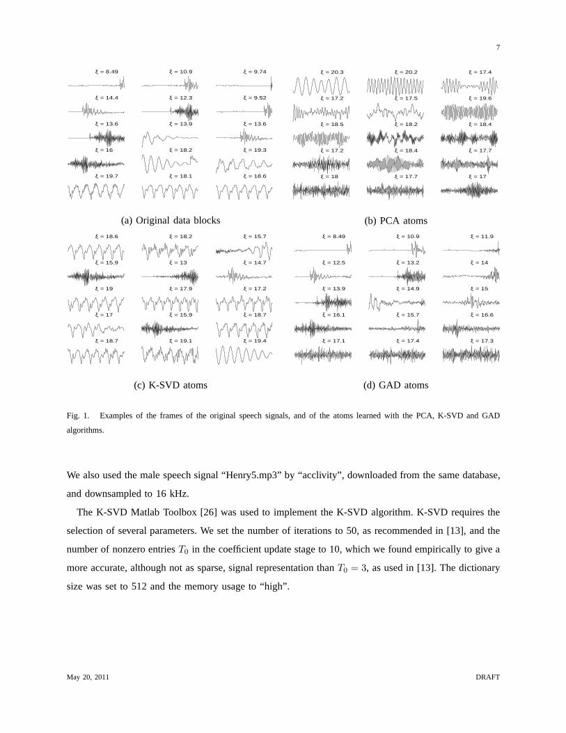
by “Corsica S”, downloaded from The Freesound Project database [25], and downsampled to 16 kHz.

May 20, 2011 DRAFT

7

ξ = 8.49 ξ = 10.9 ξ = 9.74

ξ = 14.4 ξ = 12.3 ξ = 9.52

ξ = 13.6 ξ = 13.9 ξ = 13.6

ξ = 16 ξ = 18.2 ξ = 19.3

ξ = 19.7 ξ = 18.1 ξ = 18.6

(a) Original data blocks

ξ = 20.3 ξ = 20.2 ξ = 17.4

ξ = 17.2 ξ = 17.5 ξ = 19.6

ξ = 18.5 ξ = 18.2 ξ = 18.4

ξ = 17.2 ξ = 18.4 ξ = 17.7

ξ = 18 ξ = 17.7 ξ = 17

(b) PCA atoms

ξ = 18.6 ξ = 18.2 ξ = 15.7

ξ = 15.9 ξ = 13 ξ = 14.7

ξ = 19 ξ = 17.9 ξ = 17.2

ξ = 17 ξ = 15.9 ξ = 18.7

ξ = 18.7 ξ = 19.1 ξ = 19.4

(c) K-SVD atoms

ξ = 8.49 ξ = 10.9 ξ = 11.9

ξ = 12.5 ξ = 13.2 ξ = 14

ξ = 13.9 ξ = 14.9 ξ = 15

ξ = 16.1 ξ = 15.7 ξ = 16.6

ξ = 17.1 ξ = 17.4 ξ = 17.3

(d) GAD atoms

Fig. 1. Examples of the frames of the original speech signals, and of the atoms learned with the PCA, K-SVD and GAD

algorithms.

We also used the male speech signal “Henry5.mp3” by “acclivity”, downloaded from the same database,

and downsampled to 16 kHz.

The K-SVD Matlab Toolbox [26] was used to implement the K-SVDalgorithm. K-SVD requires the

selection of several parameters. We set the number of iterations to 50, as recommended in [13], and the

number of nonzero entriesT0 in the coefficient update stage to 10, which we found empirically to give a

more accurate, although not as sparse, signal representation thanT0 = 3, as used in [13]. The dictionary

size was set to 512 and the memory usage to “high”.

May 20, 2011 DRAFT

8

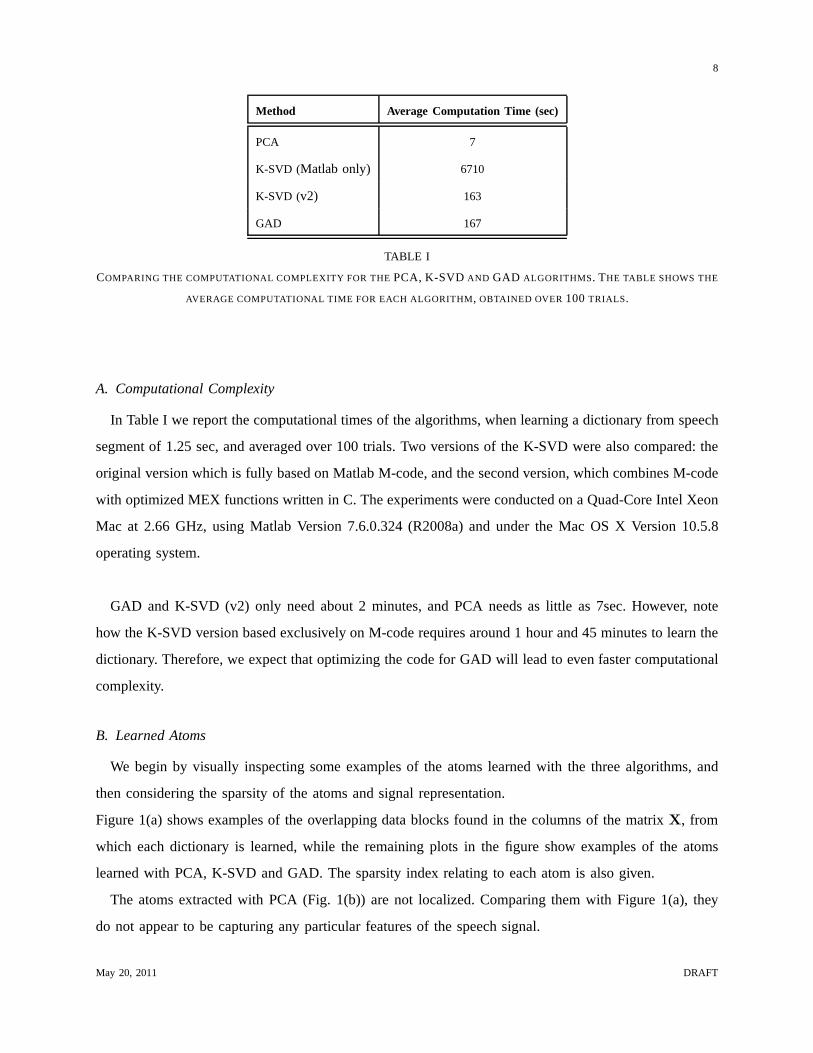
Method Average Computation Time (sec)

PCA 7

K-SVD (Matlab only) 6710

K-SVD (v2) 163

GAD 167

TABLE I

COMPARING THE COMPUTATIONAL COMPLEXITY FOR THEPCA, K-SVD AND GAD ALGORITHMS. THE TABLE SHOWS THE

AVERAGE COMPUTATIONAL TIME FOR EACH ALGORITHM, OBTAINED OVER 100 TRIALS.

A. Computational Complexity

In Table I we report the computational times of the algorithms, when learning a dictionary from speech

segment of 1.25 sec, and averaged over 100 trials. Two versions of the K-SVD were also compared: the

original version which is fully based on Matlab M-code, and the second version, which combines M-code

with optimized MEX functions written in C. The experiments were conducted on a Quad-Core Intel Xeon

Mac at 2.66 GHz, using Matlab Version 7.6.0.324 (R2008a) andunder the Mac OS X Version 10.5.8

operating system.

GAD and K-SVD (v2) only need about 2 minutes, and PCA needs as little as 7sec. However, note

how the K-SVD version based exclusively on M-code requires around 1 hour and 45 minutes to learn the

dictionary. Therefore, we expect that optimizing the code for GAD will lead to even faster computational

complexity.

B. Learned Atoms

We begin by visually inspecting some examples of the atoms learned with the three algorithms, and

then considering the sparsity of the atoms and signal representation.

Figure 1(a) shows examples of the overlapping data blocks found in the columns of the matrixX, from

which each dictionary is learned, while the remaining plotsin the figure show examples of the atoms

learned with PCA, K-SVD and GAD. The sparsity index relatingto each atom is also given.

The atoms extracted with PCA (Fig. 1(b)) are not localized. Comparing them with Figure 1(a), they

do not appear to be capturing any particular features of the speech signal.

May 20, 2011 DRAFT

9

100 200 300 400 50011

12

13

14

15

16

17

18

spar

sity

inde

x (ξ)

number of atoms

Original

PCA

SC−ICA

K−SVD

GAD

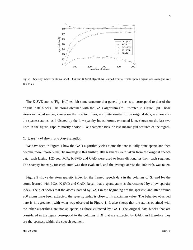
Fig. 2. Sparsity index for atoms GAD, PCA and K-SVD algorithms, learned from a female speech signal, and averaged over

100 trials.

The K-SVD atoms (Fig. 1(c)) exhibit some structure that generally seems to correspond to that of the

original data blocks. The atoms obtained with the GAD algorithm are illustrated in Figure 1(d). Those

atoms extracted earlier, shown on the first two lines, are quite similar to the original data, and are also

the sparsest atoms, as indicated by the low sparsity index. Atoms extracted later, shown on the last two

lines in the figure, capture mostly “noise”-like characteristics, or less meaningful features of the signal.

C. Sparsity of Atoms and Representation

We have seen in Figure 1 how the GAD algorithm yields atoms that are initially quite sparse and then

become more “noise”-like. To investigate this further, 100segments were taken from the original speech

data, each lasting 1.25 sec. PCA, K-SVD and GAD were used to learn dictionaries from each segment.

The sparsity indexξk for each atom was then evaluated, and the average across the 100 trials was taken.

Figure 2 shows the atom sparsity index for the framed speech data in the columns ofX, and for the

atoms learned with PCA, K-SVD and GAD. Recall that a sparse atom is characterized by a low sparsity

index. The plot shows that the atoms learned by GAD in the beginning are the sparsest, and after around

200 atoms have been extracted, the sparsity index is close toits maximum value. The behavior observed

here is in agreement with what was observed in Figure 1. It also shows that the atoms obtained with

the other algorithms are not as sparse as those extracted by GAD. The original data blocks that are

considered in the figure correspond to the columns inX that are extracted by GAD, and therefore they

are the sparsest within the speech segment.

May 20, 2011 DRAFT

10

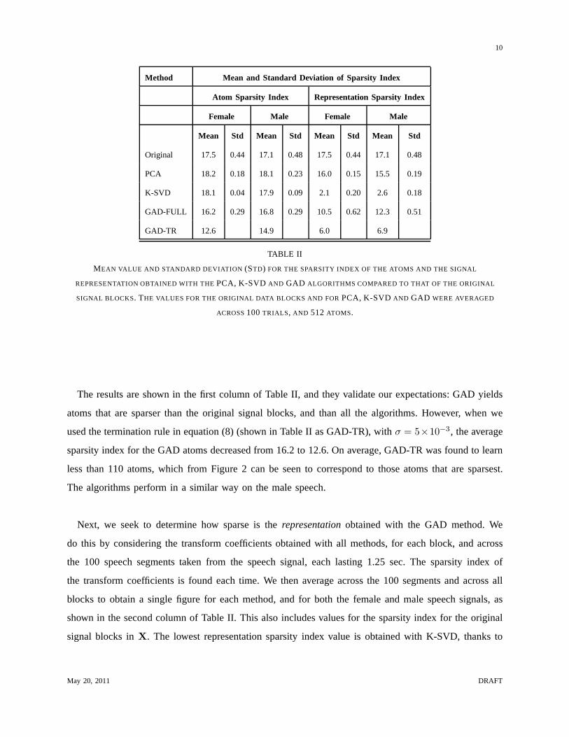
Method Mean and Standard Deviation of Sparsity Index

Atom Sparsity Index Representation Sparsity Index

Female Male Female Male

Mean Std Mean Std Mean Std Mean Std

Original 17.5 0.44 17.1 0.48 17.5 0.44 17.1 0.48

PCA 18.2 0.18 18.1 0.23 16.0 0.15 15.5 0.19

K-SVD 18.1 0.04 17.9 0.09 2.1 0.20 2.6 0.18

GAD-FULL 16.2 0.29 16.8 0.29 10.5 0.62 12.3 0.51

GAD-TR 12.6 14.9 6.0 6.9

TABLE II

MEAN VALUE AND STANDARD DEVIATION (STD) FOR THE SPARSITY INDEX OF THE ATOMS AND THE SIGNAL

REPRESENTATION OBTAINED WITH THEPCA, K-SVD AND GAD ALGORITHMS COMPARED TO THAT OF THE ORIGINAL

SIGNAL BLOCKS. THE VALUES FOR THE ORIGINAL DATA BLOCKS AND FORPCA, K-SVD AND GAD WERE AVERAGED

ACROSS100 TRIALS, AND 512 ATOMS.

The results are shown in the first column of Table II, and they validate our expectations: GAD yields

atoms that are sparser than the original signal blocks, and than all the algorithms. However, when we

used the termination rule in equation (8) (shown in Table II as GAD-TR), withσ = 5×10−3, the average

sparsity index for the GAD atoms decreased from 16.2 to 12.6.On average, GAD-TR was found to learn

less than 110 atoms, which from Figure 2 can be seen to correspond to those atoms that are sparsest.

The algorithms perform in a similar way on the male speech.

Next, we seek to determine how sparse is therepresentationobtained with the GAD method. We

do this by considering the transform coefficients obtained with all methods, for each block, and across

the 100 speech segments taken from the speech signal, each lasting 1.25 sec. The sparsity index of

the transform coefficients is found each time. We then average across the 100 segments and across all

blocks to obtain a single figure for each method, and for both the female and male speech signals, as

shown in the second column of Table II. This also includes values for the sparsity index for the original

signal blocks inX. The lowest representation sparsity index value is obtained with K-SVD, thanks to

May 20, 2011 DRAFT

11

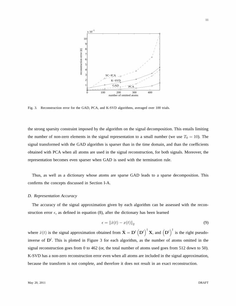
0 100 200 300 400

1

2

3

4

5

6

7

8

9

10

x 10−3

number of omitted atoms

reco

nstr

uctio

n er

ror

(ε)

SC−ICA

K−SVD

GAD PCA

Fig. 3. Reconstruction error for the GAD, PCA, and K-SVD algorithms, averaged over 100 trials.

the strong sparsity constraint imposed by the algorithm on the signal decomposition. This entails limiting

the number of non-zero elements in the signal representation to a small number (we useT0 = 10). The

signal transformed with the GAD algorithm is sparser than inthe time domain, and than the coefficients

obtained with PCA when all atoms are used in the signal reconstruction, for both signals. Moreover, the

representation becomes even sparser when GAD is used with the termination rule.

Thus, as well as a dictionary whose atoms are sparse GAD leadsto a sparse decomposition. This

confirms the concepts discussed in Section I-A.

D. Representation Accuracy

The accuracy of the signal approximation given by each algorithm can be assessed with the recon-

struction errorǫ, as defined in equation (8), after the dictionary has been learned

ǫ = ‖x(t) − x(t)‖2

(9)

wherex(t) is the signal approximation obtained fromX = Dl(

Dl)†

X, and(

Dl)†

is the right pseudo-

inverse ofDl. This is plotted in Figure 3 for each algorithm, as the numberof atoms omitted in the

signal reconstruction goes from 0 to 462 (or, the total number of atoms used goes from 512 down to 50).

K-SVD has a non-zero reconstruction error even when all atoms are included in the signal approximation,

because the transform is not complete, and therefore it doesnot result in an exact reconstruction.

May 20, 2011 DRAFT

12

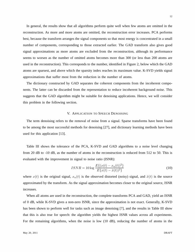
In general, the results show that all algorithms perform quite well when few atoms are omitted in the

reconstruction. As more and more atoms are omitted, the reconstruction error increases. PCA performs

best, because the transform arranges the signal componentsso that most energy is concentrated in a small

number of components, corresponding to those extracted earlier. The GAD transform also gives good

signal approximations as more atoms are excluded from the reconstruction, although its performance

seems to worsen as the number of omitted atoms becomes more than 300 (or less than 200 atoms are

used in the reconstruction). This corresponds to the number, identified in Figure 2, below which the GAD

atoms are sparsest, and above which the sparsity index reaches its maximum value. K-SVD yields signal

approximations that suffer most from the reduction in the number of atoms.

The dictionary constructed by GAD separates the coherent components from the incoherent compo-

nents. The latter can be discarded from the representation to reduce incoherent background noise. This

suggests that the GAD algorithm might be suitable for denoising applications. Hence, we will consider

this problem in the following section.

V. A PPLICATION TO SPEECHDENOISING

The term denoising refers to the removal of noise from a signal. Sparse transforms have been found

to be among the most successful methods for denoising [27], and dictionary learning methods have been

used for this application [13].

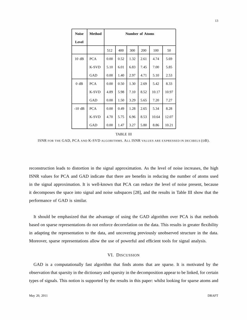
Table III shows the tolerance of the PCA, K-SVD and GAD algorithms to a noise level changing

from 20 dB to -10 dB, as the number of atoms in the reconstruction is reduced from 512 to 50. This is

evaluated with the improvement in signal to noise ratio (ISNR):

ISNR = 10 logE{(x(t) − xn(t))2}

E{x(t) − x(t))2}(10)

wherex(t) is the original signal,xn(t) is the observed distorted (noisy) signal, andx(t) is the source

approximated by the transform. As the signal approximationbecomes closer to the original source, ISNR

increases.

When all atoms are used in the reconstruction, the complete transforms PCA and GAD, yield an ISNR

of 0 dB, while K-SVD gives a non-zero ISNR, since the approximation is not exact. Generally, K-SVD

has been shown to perform well for tasks such as image denoising [7], and the results in Table III show

that this is also true for speech: the algorithm yields the highest ISNR values across all experiments.

For the remaining algorithms, when the noise is low (10 dB), reducing the number of atoms in the

May 20, 2011 DRAFT

13

Noise Method Number of Atoms

Level

512 400 300 200 100 50

10 dB PCA 0.00 0.52 1.32 2.61 4.74 5.69

K-SVD 5.10 6.01 6.83 7.45 7.00 5.85

GAD 0.00 1.40 2.97 4.71 5.10 2.53

0 dB PCA 0.00 0.50 1.30 2.69 5.42 8.33

K-SVD 4.89 5.98 7.10 8.52 10.17 10.97

GAD 0.00 1.50 3.29 5.65 7.20 7.27

-10 dB PCA 0.00 0.49 1.28 2.65 5.34 8.28

K-SVD 4.70 5.75 6.96 8.53 10.64 12.07

GAD 0.00 1.47 3.27 5.80 8.86 10.21

TABLE III

ISNR FOR THEGAD, PCA AND K-SVD ALGORITHMS. ALL ISNR VALUES ARE EXPRESSED IN DECIBELS(DB).

reconstruction leads to distortion in the signal approximation. As the level of noise increases, the high

ISNR values for PCA and GAD indicate that there are benefits inreducing the number of atoms used

in the signal approximation. It is well-known that PCA can reduce the level of noise present, because

it decomposes the space into signal and noise subspaces [28], and the results in Table III show that the

performance of GAD is similar.

It should be emphasized that the advantage of using the GAD algorithm over PCA is that methods

based on sparse representations do not enforce decorrelation on the data. This results in greater flexibility

in adapting the representation to the data, and uncovering previously unobserved structure in the data.

Moreover, sparse representations allow the use of powerfuland efficient tools for signal analysis.

VI. D ISCUSSION

GAD is a computationally fast algorithm that finds atoms thatare sparse. It is motivated by the

observation that sparsity in the dictionary and sparsity inthe decomposition appear to be linked, for certain

types of signals. This notion is supported by the results in this paper: whilst looking for sparse atoms and

May 20, 2011 DRAFT

14

making no assumptions on the decomposition, the GAD algorithm yields a signal decomposition that is

sparse.

Although the only sparsity measure considered here is the sparsity index, we have compared the

results to other measures of sparsity including the Gini index, which was found to outperform several

other sparsity measures [29]. Our experimental results indicated that the performance of the algorithm is

not noticeably different. However, we are considering to study this further in future work.

In its present form, the GAD method looks for onsets, and it might be argued that it does not take

advantage of all the possible redundancy in the speech signal, by not exploiting the pitch structure of the

signal. In future work we are considering searching for sparsity in the frequency domain, and perhaps

in prototype waveform domain [30]. On the other hand, in its present form GAD is a general algorithm

that can be used with a variety of data because it does not makeany assumptions on its characteristics.

Although the GAD algorithm is currently at the theoretical stage, it is a fast method that might in future

be used in real practical applications such as speech coding. In this case, like with PCA, this method would

require the transmission of the signal-adaptive dictionary. Other applications to which we are particularly

interested in applying the GAD method include image processing and biomedical signal processing.

Biomedical applications typically give rise to large data sets, for instance, in microarray experiments the

expression values of thousands of genes are generated. Therefore, in this case the algorithm would have

to be extended to deal with large data sets. We are also considering the application of this approach to

the problem of source separation.

VII. C ONCLUSIONS

In this paper we have presented a greedy adaptive dictionarylearning algorithm, that finds new

dictionary elements that are sparse. The algorithm constructs a signal-adaptive orthogonal dictionary,

whose atoms encode local properties of the signal.

The algorithm has been shown to yield sparse atoms and a sparse signal representation. Its performance

was compared to that of PCA and K-SVD methods, and it was foundto give good signal approximations,

even as the number of atoms in the reconstructions decreasesconsiderably.

It results in better signal reconstruction than K-SVD and ithas good tolerance to noise and does not

May 20, 2011 DRAFT

15

exhibit distortion when noise reduction is performed at lownoise levels.

VIII. A CKNOWLEDGEMENTS

The authors wish to thank the anonymous reviewers for their input that helped improving the quality

of the presentation of this work.

REFERENCES

[1] P. Foldiak, “Forming sparse representations by localanti-Hebbian learning,”Biological Cybernetics, vol. 64, pp. 165–170,

1990.

[2] B. Olshausen and D. Field, “Emergence of simple-cell receptive field properties by learning a sparse code for natural

images,”Nature, vol. 381, pp. 607–609, 1996.

[3] T. Shan and L. Jiao, “New evidences for sparse coding strategy employed in visual neurons: from the image processing

and nonlinear approximation viewpoint,” inProc. of the European Symposium on Artificial Neural Networks (ESANN),

2005, pp. 441–446.

[4] M. Zibulevsky and B. A. Pearlmutter, “Blind source separation by sparse decomposition in a signal dictionary,”Neural

Computation, vol. 13, no. 4, pp. 863–882, 2001.

[5] O. Yilmaz and S. Rickard, “Blind separation of speech mixtures via time-frequency masking,”IEEE Trans. on Signal

Processing, vol. 52, pp. 1830–1847, 2004.

[6] R. Gribonval, “Sparse decomposition of stereo signals with matching pursuit and application to blind separation ofmore

than two sources from a stereo mixture,” inProc. of the IEEE International Conference on Acoustic, Speech and Signal

Processing (ICASSP), vol. 3, 2002, pp. 3057–3060.

[7] M. Elad and M. Aharon, “Image denoising via sparse redundant representations over learned dicitonaries,”IEEE Trans.

on Image Processing, vol. 15, pp. 3736–3745, 2006.

[8] R. Gribonval and K. Schnass, “Some recovery conditions for basis learning by L1-minimization,” inProc. of the

International Symposium on Communications, Control and Signal Processing (ISCCSP), 2008, pp. 768–733.

[9] L. Rebollo-Neira, “Dictionary redundancy elimination,” IEE Proceedings - Vision, Image and Signal Processing, vol. 151,

pp. 31–34, 2004.

[10] M. S. Lewicki and T. J. Sejnowski, “Learning overcomplete representations,”Neural Computation, vol. 12, pp. 337–365,

2000.

[11] K. Kreutz-Delgado, J. Murray, D. Rao, K. Engan, T. Lee, and T. Sejnowski, “Dictionary learning algorithms for sparse

representations,”Neural Computation, vol. 15, pp. 349–396, 2003.

[12] I. Gorodnitsky, J. George, and B. Rao, “Neuromagnetic source imaging with FOCUSS: a recursive weighted minimum

norm algorithm,”Journal of Electroencephalography and Clinical Neurophysiology, vol. 95, pp. 231–251, 1995.

[13] M. Aharon, M. Elad, and A. Bruckstein, “K-SVD: An algorithm for designing overcomplete dictionaries for sparse

representations,”IEEE Trans. on Signal Processing, vol. 54, pp. 4311–4322, 2006.

[14] M. D. Plumbley, “Dictionary learning for L1-exact sparse coding,” inProc. of the International Conference on Independent

Component Analysis and Signal Separation (ICA), 2007, pp. 406–413.

[15] J. Mairal, F. Bach, J. Ponce, and G. Sapiro, “Online dictionary learning for sparse coding,” inProc. of the International

Conference on Machine Learning (ICML), vol. 382, 2009, pp. 689–696.

May 20, 2011 DRAFT

16

[16] R. Rubinstein, M. Zibulevsky, and M. Elad, “Double sparsity: Learning sparse dictionaries for sparse signal approximation,”

IEEE Trans. on Signal Processing, vol. 58, pp. 1553–1564, 2010.

[17] M. G. Jafari, E. Vincent, S. A. Abdallah, M. D. Plumbley,and M. E. Davies, “An adaptive stereo basis method for

convolutive blind audio source separation,”Neurocomputing, vol. 71, pp. 2087–2097, 2008.

[18] S. A. Abdallah and M. D. Plumbley, “If edges are the independent components of natural images, what are the independent

components of natural sounds?” inProc. of the International Conference on Independent Component Analysis and Blind

Signal Separation (ICA), 2001, pp. 534–539.

[19] M. Goodwin and M. Vetterli, “Matching pursuit and atomic signal models based on recursive filter banks,”IEEE Trans.

on Signal Processing, vol. 47, pp. 1890–1902, 1999.

[20] V. Tan and C. Fevotte, “A study of the effect of source sparsity for various transforms on blind audio source separation

performance,” inProc. of the Workshop on Signal Processing with Adaptative Sparse Structured Representations (SPARS),

2005.

[21] M. Jafari and M. Plumbley, “An adaptive orthogonal sparsifying transform for speech signals,” inProc. of the International

Symposium on Communications, Control and Signal Processing (ISCCSP), 2008, pp. 786–790.

[22] S. Mallat and Z. Zhang, “Matching pursuit with time-frequency dictionaries,”IEEE Trans. on Signal Processing, vol. 41,

pp. 3397–3415, 1993.

[23] S. Mallat, G. Davis, and Z. Zhang, “Adaptive time-frequency decompositions,”SPIE Journal of Optical Engineering,

vol. 33, pp. 2183–2191, 1994.

[24] S. Haykin,Neural networks: a comprehensive foundation, 2nd ed. Prentice Hall, 1999.

[25] “The Freesound Project. A collaborative database of Creative Commons licensed sounds.” [Online]. Available:

www.freesound.org

[26] R. Rubinstein. [Online]. Available: www.cs.technion.ac.il/∼ronrubin/ software.html

[27] S. Valiollahzadeh, H. Firouzi, M. Babaie-Zadeh, and C.Jutten, “Image denoising using sparse representations,” in Proc.

of the International Conference on Independent Component Analysis and Signal Separation (ICA), 2009, pp. 557–564.

[28] A. Hyvaerinen, J. Karhunen, and E. Oja,Independent Component Analysis. John Wiley & Sons, 2000.

[29] N. Hurley and S. Rickard, “Comparing measures of sparsity,” IEEE Trans. on Information Theory, vol. 55, pp. 4723–4741,

2009.

[30] W. B. Kleijn, “Encoding speech using prototype waveforms,” IEEE Trans. on Speech and Audio Processing, vol. 4, pp.

386–399, 1993.

May 20, 2011 DRAFT

17

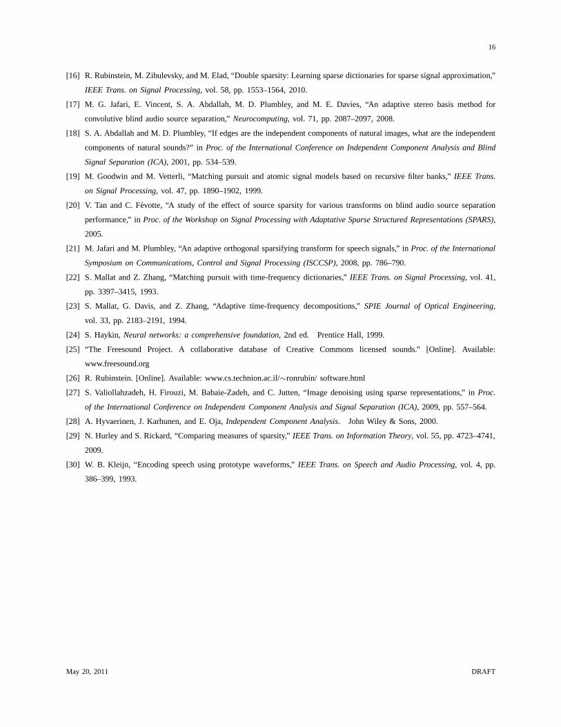
Maria G. Jafari (S’01–M’02) received the M.Eng. (Hons.) degree in electrical and electronic engineering

from Imperial College London, U.K., in 1999 and the Ph.D. degree in signal processing from King’s

College London, U.K. in 2003. From 2002 to 2004 she worked as aResearch Associate at King’s College

London, where her research focused on the application of signal processing to biomedical problems. In

June 2004, she joined the Centre for Digital Music, Queen Mary University of London, U.K., where she

is currently a Research Assistant. Her research interest are in the areas of blind signal separation, sparse

representations and dictionary learning. She especially interested in the application of these and other techniques to speech and

music processing and the analysis of other audio sounds, such as heart and bowel sounds.

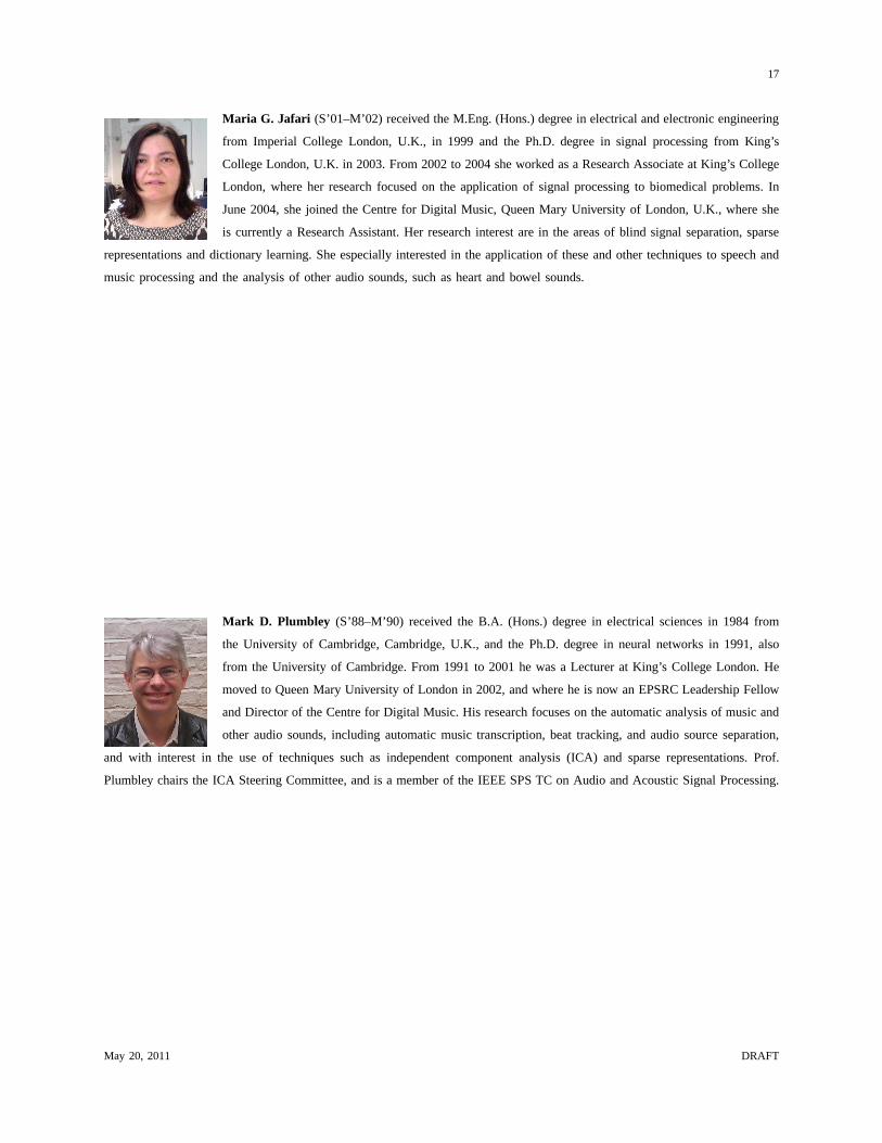
Mark D. Plumbley (S’88–M’90) received the B.A. (Hons.) degree in electricalsciences in 1984 from

the University of Cambridge, Cambridge, U.K., and the Ph.D.degree in neural networks in 1991, also

from the University of Cambridge. From 1991 to 2001 he was a Lecturer at King’s College London. He

moved to Queen Mary University of London in 2002, and where heis now an EPSRC Leadership Fellow

and Director of the Centre for Digital Music. His research focuses on the automatic analysis of music and

other audio sounds, including automatic music transcription, beat tracking, and audio source separation,

and with interest in the use of techniques such as independent component analysis (ICA) and sparse representations. Prof.

Plumbley chairs the ICA Steering Committee, and is a member of the IEEE SPS TC on Audio and Acoustic Signal Processing.

May 20, 2011 DRAFT