Fast Anytime Motion Planning in Point Clouds by

Fast Anytime Motion Planning in Point Clouds byInterleaving Sampling and Interior Point Optimization

Alan Kuntz, Chris Bowen, and Ron Alterovitz

University of North Carolina at Chapel HillChapel Hill, NC 27599-3175, USA

{adkuntz,cbbowen,ron}@cs.unc.edu

Abstract. Robotic manipulators operating in unstructured environments such ashomes and offices need to plan their motions quickly while relying on real-worldsensors, which typically produce point clouds. To enable intuitive, interactive, andreactive user interfaces, the motion plan computation should provide high-qualitysolutions quickly and in an anytime manner, meaning the algorithm progressivelyimproves its solution and can be interrupted at any time and return a valid solu-tion. To address these challenges, we combine two paradigms: (1) asymptotically-optimal sampling-based motion planning, which is effective at providing anytimesolutions but can struggle to quickly converge to high quality solutions in high di-mensional configuration spaces, and (2) optimization, which locally refines pathsquickly. We propose the use of interior point optimization for its ability to performin an anytime manner that guarantees obstacle avoidance in each iteration, and weprovide a novel lazy formulation that efficiently operates directly on point clouddata. Our method iteratively alternates between anytime sampling-based motionplanning and anytime, lazy interior point optimization to compute high qualitymotion plans quickly, converging to a globally optimal solution.

1 Introduction

Robotic manipulators are entering unstructured environments, such as homes, offices,hospitals, and restaurants, where robots need to plan motions quickly while ensuringsafety via obstacle avoidance. Motion planning in such settings is challenging in part be-cause the robot must rely on real-world sensors such as laser scanners, RGBD sensors,or stereo reconstruction, which typically produce point clouds. In addition, enabling in-tuitive, interactive, and reactive user experiences requires that the robot generate plansof high quality as quickly as possible, without necessarily knowing in advance the max-imum time allocatable to motion planning. Hence, motion planning in such settingsshould be implemented as an anytime algorithm, meaning the algorithm progressivelyimproves its solution and can be interrupted at any time and return a valid solution.

To enable fast, anytime, asymptotically-optimal motion planning in point clouds, wepropose to blend two popular motion planning paradigms: (1) sampling-based motionplanning and (2) optimization-based motion planning. Sampling-based motion plannerscan directly use point cloud data by incorporating appropriate collision detection algo-rithms [19] and can optimize a cost metric in an asymptotically optimal manner [12].

2 Alan Kuntz, Chris Bowen, and Ron Alterovitz

However, sampling-based motion planners in practice can be slow to converge and fre-quently return paths in finite time that are far from optimal, especially for problems withhigher dimensional configuration spaces [10]. In contrast, optimization-based motionplanners are often very fast [21, 23, 20, 11], but typically do not converge to globallyoptimal solutions, do not operate in an anytime manner (since, even when initializedwith a feasible solution, their intermediate iterations may consider robot configurationsthat are in collision with obstacles), and are inefficient when using large point clouds.In this paper, we introduce a new optimization approach to motion planning based oninterior point optimization [25, 24], which has unique properties that enable anytimemotion planning and efficient handling of large point clouds. By integrating our newinterior point optimization formulation with a sampling-based method, our approachquickly computes locally optimized plans in an anytime fashion, and continues to re-fine the solution toward global optimality for as long as time allows.

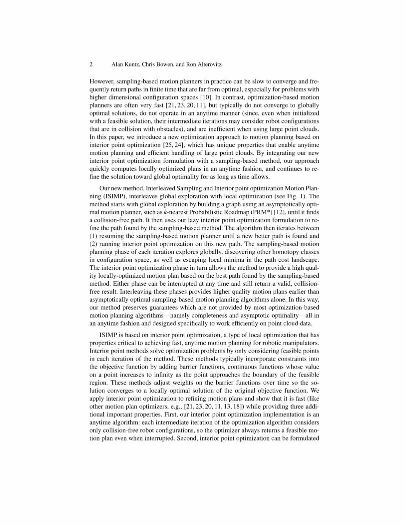
Our new method, Interleaved Sampling and Interior point optimization Motion Plan-ning (ISIMP), interleaves global exploration with local optimization (see Fig. 1). Themethod starts with global exploration by building a graph using an asymptotically opti-mal motion planner, such as k-nearest Probabilistic Roadmap (PRM*) [12], until it findsa collision-free path. It then uses our lazy interior point optimization formulation to re-fine the path found by the sampling-based method. The algorithm then iterates between(1) resuming the sampling-based motion planner until a new better path is found and(2) running interior point optimization on this new path. The sampling-based motionplanning phase of each iteration explores globally, discovering other homotopy classesin configuration space, as well as escaping local minima in the path cost landscape.The interior point optimization phase in turn allows the method to provide a high qual-ity locally-optimized motion plan based on the best path found by the sampling-basedmethod. Either phase can be interrupted at any time and still return a valid, collision-free result. Interleaving these phases provides higher quality motion plans earlier thanasymptotically optimal sampling-based motion planning algorithms alone. In this way,our method preserves guarantees which are not provided by most optimization-basedmotion planning algorithms—namely completeness and asymptotic optimality—all inan anytime fashion and designed specifically to work efficiently on point cloud data.

ISIMP is based on interior point optimization, a type of local optimization that hasproperties critical to achieving fast, anytime motion planning for robotic manipulators.Interior point methods solve optimization problems by only considering feasible pointsin each iteration of the method. These methods typically incorporate constraints intothe objective function by adding barrier functions, continuous functions whose valueon a point increases to infinity as the point approaches the boundary of the feasibleregion. These methods adjust weights on the barrier functions over time so the so-lution converges to a locally optimal solution of the original objective function. Weapply interior point optimization to refining motion plans and show that it is fast (likeother motion plan optimizers, e.g., [21, 23, 20, 11, 13, 18]) while providing three addi-tional important properties. First, our interior point optimization implementation is ananytime algorithm: each intermediate iteration of the optimization algorithm considersonly collision-free robot configurations, so the optimizer always returns a feasible mo-tion plan even when interrupted. Second, interior point optimization can be formulated

Fast Anytime Motion Planning in Point Clouds 3

S G

(a) Sampled First Path

S G

(b) Optimized First Path

S G

(c) Sampled Second Path

S G

(d) Optimized Second Path (e) Sampled Path on Baxter (f) Optimized Path on Baxter

Fig. 1. ISIMP interleaves sampling-based and optimization-based motion planning. (a) ISIMPfirst performs sampling-based motion planning until a feasible motion plan is found from start togoal. (b) It then uses interior point optimization to locally optimize the plan. (c) Sampling-basedmotion planning resumes until a shorter plan is found. (d) The shorter plan is then optimized.The method iterates in this fashion and can be interrupted at any time after step (a) and returna feasible solution that gets better over time. (e) An example sampling-based plan found for aBaxter robot in a point cloud sensed by Microsoft Kinect. (f) That plan locally optimized.

to efficiently and directly handle large point clouds, which we accomplish using a lazyevaluation of constraints. This eliminates the time-consuming process of transform-ing the point cloud into more complex geometric primitives or meshes, which is oftenrequired by other optimization-based motion planners to be efficient. Third, our inte-rior point optimization is designed to optimize path length, a commonly desired metricwhich is often used by sampling-based motion planners. Many existing optimization-based motion planners [21, 23, 20, 11] are designed to optimize metrics such as smooth-ness, which do not satisfy the triangle inequality and hence are incompatible with costrequirements of asymptotically-optimal sampling-based motion planners.

We evaluate the efficacy of ISIMP for a Baxter robot’s manipulator arm using aMicrosoft Kinect to sense point cloud data in a cluttered environment. We demonstrateISIMP’s fast, anytime, and asymptotically optimal performance in comparison to othermotion planners that only use either sampling or local optimization.

2 Related Work

In sampling-based motion planning, a graph data structure is constructed incrementallyvia random sampling providing a collision-free tree or roadmap in the robot’s configu-ration space. These algorithms provide probabilistic completeness, i.e., the probabilityof finding a path, if one exists, approaches one as the number of samples approaches in-finity. Examples include the Rapidly-exploring Random Tree (RRT) [16] and the Prob-


abilistic Roadmap (PRM) [13] methods. These methods have been adapted in manyways, including to take advantage of structure in the robot’s configuration space and bymodifying the sampling strategy [6, 15].

Adaptations of these algorithms can provide asymptotic optimality guarantees inwhich the path cost (e.g., path length) will approach the global optimum as the num-ber of algorithm iterations increases. Examples include RRT* and PRM* [12] where theunderlying motion planning graph is either rewired or has asymptotically changing con-nection strategies. Other asymptotically optimal algorithms grow a tree in cost-to-arrivespace [10], identify vertices likely to be a part of an optimal path [1], or investigate thedistributions from which samples and trajectories are taken [14]. Lazy collision check-ing has been shown to substantially improve the speed of these algorithms [9], and insome cases, near optimality can be achieved while improving speed [22, 7].

Optimization-based motion planning algorithms perform numerical optimization ina high dimensional trajectory space. Each trajectory is typically encoded as a vectorof parameters representing a sequence of robot configurations or controls. A cost canbe computed for each trajectory, and the motion planner’s goal is to compute a trajec-tory that minimizes cost. In the presence of obstacles and other constraints, the prob-lem can be formulated and solved as a numerical optimization problem. Examples in-clude taking an initial trajectory and performing gradient descent [21], using sequentialquadratic programming with inequality constraints to locally optimize trajectories [23],and combining optimization with re-planning to account for dynamic obstacles [20].These methods typically produce high quality paths but are frequently unable to escapelocal minima, and as such are subject to initialization concerns. To avoid local minima,some methods inject randomness [11, 3]. The solutions of these existing optimization-based motion planners may converge to locally optimal motion plans that include robotconfigurations that are in collision with obstacles. This limitation can be partially cir-cumvented through techniques such as restarting the optimization with multiple differ-ent initial paths (e.g., [23]), but such approaches are heuristic and provide no guaranteethat a collision-free trajectory will be found in general.

Several methods aim to bridge the gap between sampling-based methods and opti-mization. Some methods use paths generated by global planners and refine them usingshortcutting or smoothing methods adaptively or in post processing [18, 8]. GradienT-RRT moves vertices to lower cost regions using gradient descent during the constructionof an RRT [2]. More recently, local optimization has been used on in-collision edgesduring sampling-based planning to bring them out of collision and effectively find nar-row passages [4]. In contrast, our method is using the local optimizer not to find narrowpassages, but to improve the overall quality of the paths found by the sampling-basedplanner, while relying on the sampling-based planner’s completeness property to dis-cover narrow passages. BiRRT-Opt [17] utilizes a bi-directional RRT to generate aninitial trajectory for trajectory optimization, demonstrating the efficacy of a collision-free initial solution for local optimization. Our method differs in that interior point opti-mization provides collision-free iterates allowing it to work in an anytime fashion, andour method continues beyond a single local optimization to provide global asymptoticoptimality.


3 Problem Definition

Let C be the configuration space of the robot. Let q ∈ C represent a single robot con-figuration of dimensionality d and Π = {q0,q1, . . . ,qn−1} represent a continuous pathin configuration space in a piecewise linear manner by a sequence of n configurations.Such paths may need to satisfy generalized, user-defined inequality constraints. Theseconstraints could include joint limits, end effector orientation requirements, etc, whereeach constraint may be represented by the inequality g(Π) ≥ 0 for some constraintspecific function g. Let the set of all such user-defined constraints be J.

In the robot’s workspace are obstacles that must be avoided, and which are beingrepresented by a point cloud. We consider each point in the point cloud an obstacleand let the set of all such points be O. We also define the robot’s geometry as a set ofgeometric primitives S. An individual geometric primitive s ∈ S could be represented asa mesh, bounding sphere, capsule, etc.

A path is collision-free if the robot’s geometry S over each edge (qi,qi+1), i =0, . . . ,n− 2, does not intersect an obstacle o ∈ O. Formally, we require a functionclearance(qi,qi+1,s,o) which is a function parameterized by a path edge (qi,qi+1),a geometric primitive s, and an obstacle o. This function, formally defined in Sec. 4,is continuous and monotonically increasing, has positive value when o is not in col-lision with s over the edge, negative value when o penetrates into s on the edge, and0 at the boundary. A collision-free path then becomes a path for which each edgehas non-negative clearance for all o ∈ O and s ∈ S. This requirement can be repre-sented as an additional set of inequality constraints, which we define as K, whereinclearance(qi,qi+1,s,o)≥ 0, for all o ∈ O and s ∈ S.

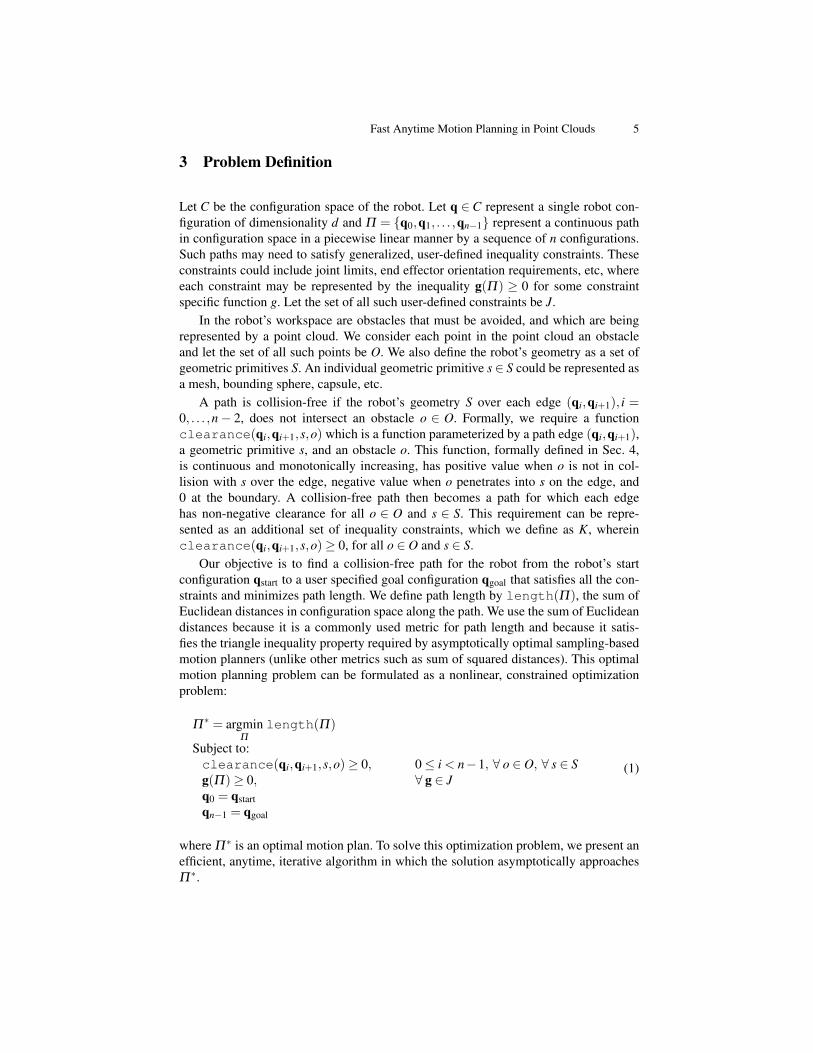
Our objective is to find a collision-free path for the robot from the robot’s startconfiguration qstart to a user specified goal configuration qgoal that satisfies all the con-straints and minimizes path length. We define path length by length(Π), the sum ofEuclidean distances in configuration space along the path. We use the sum of Euclideandistances because it is a commonly used metric for path length and because it satis-fies the triangle inequality property required by asymptotically optimal sampling-basedmotion planners (unlike other metrics such as sum of squared distances). This optimalmotion planning problem can be formulated as a nonlinear, constrained optimizationproblem:

Π∗ = argmin

Π

length(Π)

Subject to:clearance(qi,qi+1,s,o)≥ 0, 0≤ i < n−1, ∀ o ∈ O, ∀ s ∈ Sg(Π)≥ 0, ∀ g ∈ Jq0 = qstartqn−1 = qgoal

(1)

where Π ∗ is an optimal motion plan. To solve this optimization problem, we present anefficient, anytime, iterative algorithm in which the solution asymptotically approachesΠ ∗.


4 Method

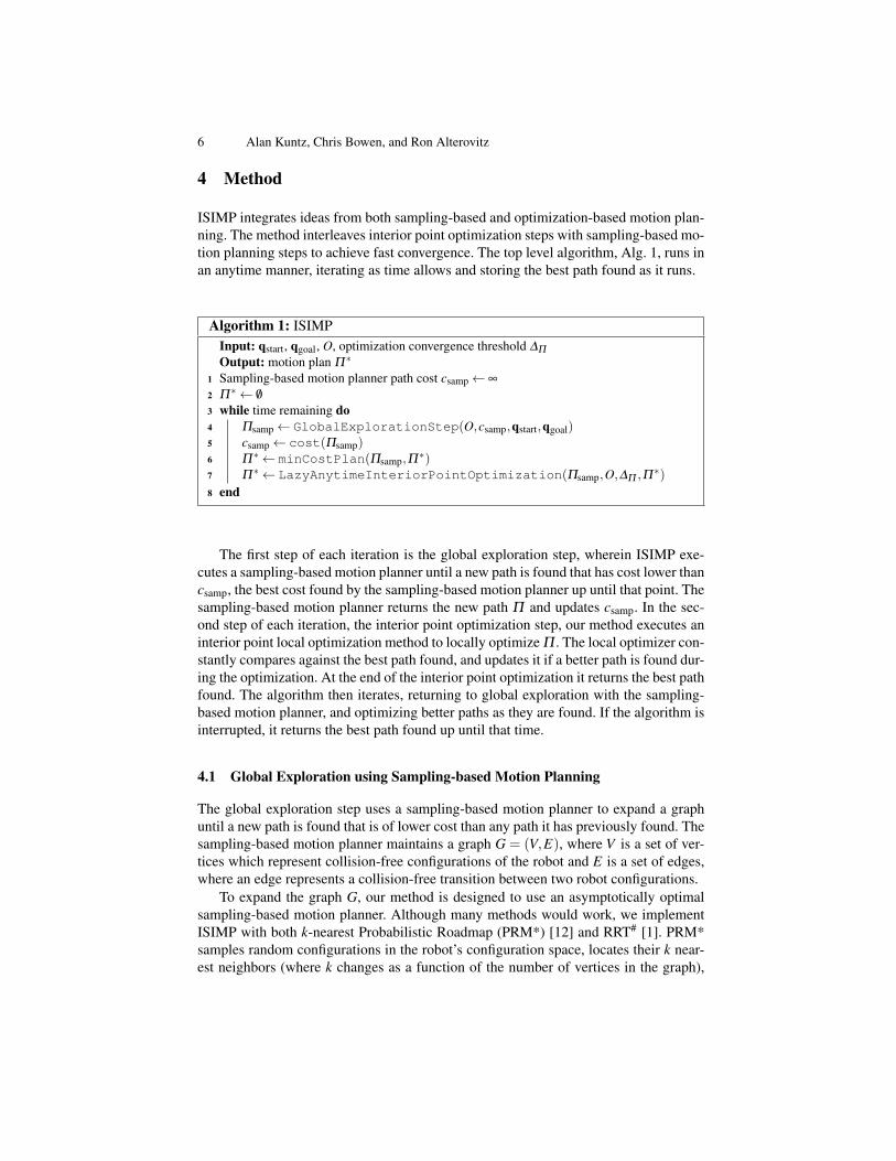
ISIMP integrates ideas from both sampling-based and optimization-based motion plan-ning. The method interleaves interior point optimization steps with sampling-based mo-tion planning steps to achieve fast convergence. The top level algorithm, Alg. 1, runs inan anytime manner, iterating as time allows and storing the best path found as it runs.

Algorithm 1: ISIMPInput: qstart, qgoal, O, optimization convergence threshold ∆Π

Output: motion plan Π∗

1 Sampling-based motion planner path cost csamp← ∞

2 Π∗← /03 while time remaining do4 Πsamp← GlobalExplorationStep(O,csamp,qstart,qgoal)5 csamp← cost(Πsamp)6 Π∗← minCostPlan(Πsamp,Π

∗)7 Π∗← LazyAnytimeInteriorPointOptimization(Πsamp,O,∆Π ,Π∗)

8 end

The first step of each iteration is the global exploration step, wherein ISIMP exe-cutes a sampling-based motion planner until a new path is found that has cost lower thancsamp, the best cost found by the sampling-based motion planner up until that point. Thesampling-based motion planner returns the new path Π and updates csamp. In the sec-ond step of each iteration, the interior point optimization step, our method executes aninterior point local optimization method to locally optimize Π . The local optimizer con-stantly compares against the best path found, and updates it if a better path is found dur-ing the optimization. At the end of the interior point optimization it returns the best pathfound. The algorithm then iterates, returning to global exploration with the sampling-based motion planner, and optimizing better paths as they are found. If the algorithm isinterrupted, it returns the best path found up until that time.

4.1 Global Exploration using Sampling-based Motion Planning

The global exploration step uses a sampling-based motion planner to expand a graphuntil a new path is found that is of lower cost than any path it has previously found. Thesampling-based motion planner maintains a graph G = (V,E), where V is a set of ver-tices which represent collision-free configurations of the robot and E is a set of edges,where an edge represents a collision-free transition between two robot configurations.

To expand the graph G, our method is designed to use an asymptotically optimalsampling-based motion planner. Although many methods would work, we implementISIMP with both k-nearest Probabilistic Roadmap (PRM*) [12] and RRT# [1]. PRM*samples random configurations in the robot’s configuration space, locates their k near-est neighbors (where k changes as a function of the number of vertices in the graph),


and attempts to connect the configurations to each of its neighbors. RRT# is a state-of-the-art asymptotically optimal sampling-based motion planner, which incrementallybuilds a tree identifying which vertices are likely to belong to an optimal path. In eachglobal exploration step, the asymptotically optimal sampling based motion planner ex-ecutes until it finds a collision-free path better than the current best, at which point theoptimization step begins.

4.2 Lazy Interior Point Optimization

Local optimization for motion planning is typically performed by constructing a highdimensional vector out of the state variables of the problem to be optimized. In ourcase, this would be a vector representing the motion plan we are optimizing, i.e. ifwe have a path with n configurations of dimensionality d, then each motion plan canbe represented as an n× d dimensional vector. Optimization can then be viewed asiteratively moving this vector through its high dimensional space to minimize the cost.In the case of constrained optimization, there are regions of this space which representareas where the constraints are satisfied (i.e., feasible or unconstrained space) and areaswhere the constraints are not satisfied (i.e., infeasible or constrained space).

Many other classes of optimization methods (such as penalty methods and sequen-tial quadratic programming) allow their intermediate solutions to move through infeasi-ble space, i.e. collide with obstacles or violate joint limits, with the hope that the even-tual locally optimal solution is feasible. Interior point methods, by contrast, require theirintermediate solutions to always be feasible [25, 24]. This is typically accomplishedthrough the use of barrier functions. A barrier function works by introducing a continu-ous function whose value approaches infinity at the edge of the constrained space. Theintermediate iterations of optimization are then influenced by the barrier functions toavoid the constrained regions. As the optimization iterates, the width of these barrierfunctions is reduced such that the solution is allowed to approach the constrained spacebut not to enter it. This is the property that we leverage to create an anytime solutioninside the optimization framework. Each intermediate solution of the optimization isalways a collision-free motion plan and as such can be returned early if necessary.

We build an interior point optimization framework around a black box interior pointoptimizer. The optimizer is responsible for generating intermediate, feasible solutions,and our framework updates the state for the optimizer as a function of those intermediatesolutions to allow for faster computation. Details of our lazy interior point optimizationframework can be seen in Alg. 2.

We optimize our paths with respect to path length. The collision avoidance con-straints are formulated over each edge in the path, i.e. the linear interpolation throughconfiguration space between the two configurations. We define our clearance function(as in equation (1)) as a function of the minimum distance between the point in thepoint cloud and the geometric primitive interpolated through the workspace as deter-mined by the robot’s forward kinematics. This formulation generates a large number ofconstraints (# of robot geometric primitives× # of edges in the path× # of points in thepoint cloud). Because the optimization must consider each constraint, fewer constraintsresults in quicker optimization times. In the following paragraphs, we discuss our novel


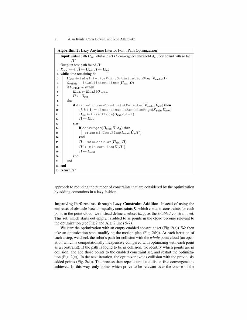
Algorithm 2: Lazy Anytime Interior Point Path OptimizationInput: initial path Πinit, obstacle set O, convergence threshold ∆Π , best found path so far

Π∗

Output: best path found Π∗

1 Kenab← /0, Π ←Πinit, Π ←Πinit2 while time remaining do3 Πnext← takeInteriorPointOptimizationStep(Kenab,Π)4 Ocollide← inCollisionPoints(Πnext,O)5 if Ocollide 6= /0 then6 Kenab← Kenab

⋃Ocollide

7 Π ←Πinit8 else9 if discontinuousConstraintDetected(Kenab,Πnext) then

10 {k,k+1}= discontinuousJacobianEdge(Kenab,Πnext)11 Πinit← bisectEdge(Πinit,k,k+1)12 Π ←Πinit13 else14 if converged(Πnext,Π ,∆π ) then15 return minCostPlan(Πnext,Π ,Π∗)16 end17 Π ← minCostPlan(Πnext,Π)

18 Π∗← minCostPlan(Π ,Π∗)19 Π ←Πnext

20 end21 end22 end23 return Π∗

approach to reducing the number of constraints that are considered by the optimizationby adding constraints in a lazy fashion.

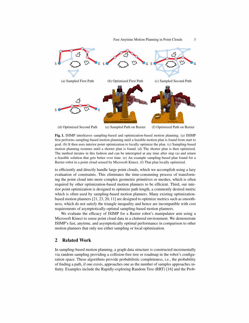
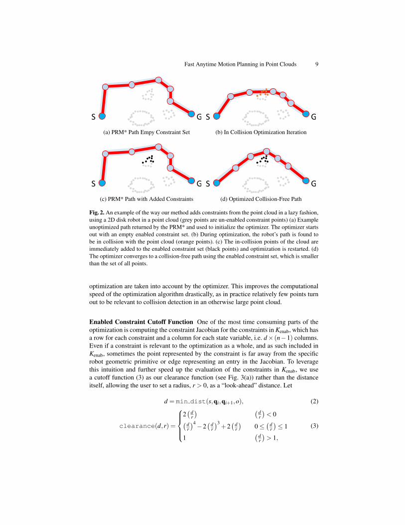
Improving Performance through Lazy Constraint Addition Instead of using theentire set of obstacle-based inequality constraints K, which contains constraints for eachpoint in the point cloud, we instead define a subset Kenab as the enabled constraint set.This set, which starts out empty, is added to as points in the cloud become relevant tothe optimization (see Fig 2 and Alg. 2 lines 5-7).

We start the optimization with an empty enabled constraint set (Fig. 2(a)). We thentake an optimization step, modifying the motion plan (Fig. 2(b)). At each iteration ofsuch a step, we check the robot’s path for collision with the whole point cloud (an oper-ation which is computationally inexpensive compared with optimizing with each pointas a constraint). If the path is found to be in collision, we identify which points are incollision, and add those points to the enabled constraint set, and restart the optimiza-tion (Fig. 2(c)). In the next iteration, the optimizer avoids collision with the previouslyadded points (Fig. 2(d)). The process then repeats until a collision-free convergence isachieved. In this way, only points which prove to be relevant over the course of the


S G(a) PRM* Path Empy Constraint Set

S G(b) In Collision Optimization Iteration

S G(c) PRM* Path with Added Constraints

S G(d) Optimized Collision-Free Path

Fig. 2. An example of the way our method adds constraints from the point cloud in a lazy fashion,using a 2D disk robot in a point cloud (grey points are un-enabled constraint points) (a) Exampleunoptimized path returned by the PRM* and used to initialize the optimizer. The optimizer startsout with an empty enabled constraint set. (b) During optimization, the robot’s path is found tobe in collision with the point cloud (orange points). (c) The in-collision points of the cloud areimmediately added to the enabled constraint set (black points) and optimization is restarted. (d)The optimizer converges to a collision-free path using the enabled constraint set, which is smallerthan the set of all points.

optimization are taken into account by the optimizer. This improves the computationalspeed of the optimization algorithm drastically, as in practice relatively few points turnout to be relevant to collision detection in an otherwise large point cloud.

Enabled Constraint Cutoff Function One of the most time consuming parts of theoptimization is computing the constraint Jacobian for the constraints in Kenab, which hasa row for each constraint and a column for each state variable, i.e. d× (n−1) columns.Even if a constraint is relevant to the optimization as a whole, and as such included inKenab, sometimes the point represented by the constraint is far away from the specificrobot geometric primitive or edge representing an entry in the Jacobian. To leveragethis intuition and further speed up the evaluation of the constraints in Kenab, we usea cutoff function (3) as our clearance function (see Fig. 3(a)) rather than the distanceitself, allowing the user to set a radius, r > 0, as a “look-ahead” distance. Let

d = min dist(s,qi,qi+1,o), (2)

clearance(d,r) =

2( d

r

) ( dr

)< 0( d

r

)4−2( d

r

)3+2( d

r

)0≤

( dr

)≤ 1

1( d

r

)> 1,

(3)


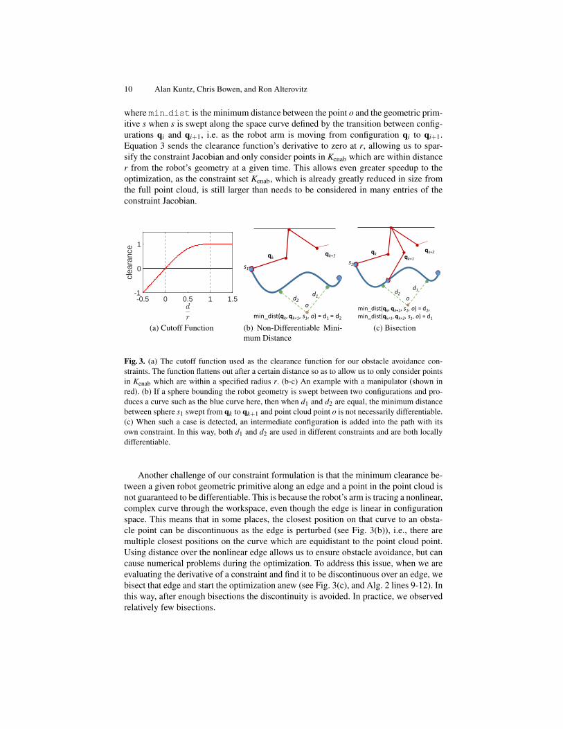
where min dist is the minimum distance between the point o and the geometric prim-itive s when s is swept along the space curve defined by the transition between config-urations qi and qi+1, i.e. as the robot arm is moving from configuration qi to qi+1.Equation 3 sends the clearance function’s derivative to zero at r, allowing us to spar-sify the constraint Jacobian and only consider points in Kenab which are within distancer from the robot’s geometry at a given time. This allows even greater speedup to theoptimization, as the constraint set Kenab, which is already greatly reduced in size fromthe full point cloud, is still larger than needs to be considered in many entries of theconstraint Jacobian.

-0.5 0 0.5 1 1.5d

r

-1

0

1

clea

ranc

e

(a) Cutoff Function

o

qk qk+1

d1d2

s1

min_dist(qk,qk+1,s1, o)=d1 =d2(b) Non-Differentiable Mini-mum Distance

o

qk qk+2

d1d2

s1

min_dist(qk,qk+1,s1, o)=d2,min_dist(qk+1,qk+2,s1, o)=d1

qk+1

(c) Bisection

Fig. 3. (a) The cutoff function used as the clearance function for our obstacle avoidance con-straints. The function flattens out after a certain distance so as to allow us to only consider pointsin Kenab which are within a specified radius r. (b-c) An example with a manipulator (shown inred). (b) If a sphere bounding the robot geometry is swept between two configurations and pro-duces a curve such as the blue curve here, then when d1 and d2 are equal, the minimum distancebetween sphere s1 swept from qk to qk+1 and point cloud point o is not necessarily differentiable.(c) When such a case is detected, an intermediate configuration is added into the path with itsown constraint. In this way, both d1 and d2 are used in different constraints and are both locallydifferentiable.

Another challenge of our constraint formulation is that the minimum clearance be-tween a given robot geometric primitive along an edge and a point in the point cloud isnot guaranteed to be differentiable. This is because the robot’s arm is tracing a nonlinear,complex curve through the workspace, even though the edge is linear in configurationspace. This means that in some places, the closest position on that curve to an obsta-cle point can be discontinuous as the edge is perturbed (see Fig. 3(b)), i.e., there aremultiple closest positions on the curve which are equidistant to the point cloud point.Using distance over the nonlinear edge allows us to ensure obstacle avoidance, but cancause numerical problems during the optimization. To address this issue, when we areevaluating the derivative of a constraint and find it to be discontinuous over an edge, webisect that edge and start the optimization anew (see Fig. 3(c), and Alg. 2 lines 9-12). Inthis way, after enough bisections the discontinuity is avoided. In practice, we observedrelatively few bisections.


4.3 Asymptotic Optimality

Asymptotic optimality of our method falls naturally from the use of an asymptoticallyoptimal motion planner as the underlying sampling-based motion planner, as long asthree conditions are met.

1. The sampling-based motion planner adds at least one node to its roadmap betweenadjacent interior point optimization calls.

2. The interior point optimization does not make the roadmap’s solution worse.3. The interior point optimization completes in finite time.

The first is dependent on the implementation of the sampling-based motion planner.The implementations we use guarantee this property. The second can be handled bydiscarding any solutions which are worse than the best that has been found at any pointin time. The third can be guaranteed with an external time limiter on the optimization.

5 Results

We implement the sampling-based motion planning portion of our method using theOMPL framework [5], including OMPL’s PRM* and RRT# implementations. For thepurposes of this section, we will refer to ISIMP with PRM* as ISIMP, and ISIMPwith RRT# as ISIMP-#. For the black box local optimizer, we use the IPOPT softwareframework, an open source interior point optimization library1 [24].

We consider a scenario involving motion planning for the left arm of a Baxter robot(see Fig. 6). For the purposes of computing constraints in the optimization and obsta-cle avoidance in the sampling-based motion planner, we represent the geometry of therobotic manipulator arm as a set of 9 bounding spheres along the links of the robot’sarm. The choice of bounding spheres allows us to conservatively represent the robot’sgeometry while enabling fast distance calculations between the geometric primitivesand the points in the point cloud.

We evaluate ISIMP’s performance in a real-world point cloud obtained from a Mi-crosoft Kinect sensor (see Fig 6). We evaluate our method utilizing point clouds ofdiffering sizes, ≈ 10,000 points, ≈ 25,000 points, and ≈ 100,000 points, the smallerof which were generated via downsampling the original point cloud. We generated 50motion planning scenarios at random in the scene using random start and goal config-urations, using rejection sampling to remove trivial scenarios for which a straight-linenaive trajectory would not collide with the point cloud.

We compare our method to the popular anytime asymptotically-optimal samplingbased motion planners PRM* [12] and RRT# [1] using OMPL [5], and to a populartrajectory optimization method, Traj-Opt [23], using their distributed source code. Allresults were generated on an 3.40GHz Intel Xeon E5-1680 CPU with 64GB of RAM.

1IPOPT requires definitions of a cost function to be minimized (path length in our case),constraint functions (J and K or Kenab), and cost and constraint Jacobians. It then handles theoptimization iterations itself. Note that default settings will allow intermediate solutions to po-tentially exist in infeasible space. We set the settings to prevent infeasible intermediate solutions.


5.1 Comparison to Asymptotically-optimal Sampling-based Motion Planners

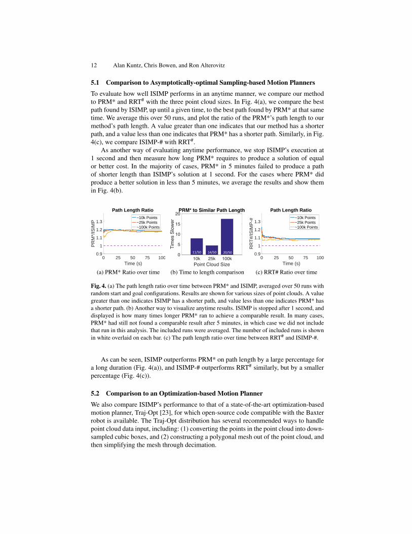
To evaluate how well ISIMP performs in an anytime manner, we compare our methodto PRM* and RRT# with the three point cloud sizes. In Fig. 4(a), we compare the bestpath found by ISIMP, up until a given time, to the best path found by PRM* at that sametime. We average this over 50 runs, and plot the ratio of the PRM*’s path length to ourmethod’s path length. A value greater than one indicates that our method has a shorterpath, and a value less than one indicates that PRM* has a shorter path. Similarly, in Fig.4(c), we compare ISIMP-# with RRT#.

As another way of evaluating anytime performance, we stop ISIMP’s execution at1 second and then measure how long PRM* requires to produce a solution of equalor better cost. In the majority of cases, PRM* in 5 minutes failed to produce a pathof shorter length than ISIMP’s solution at 1 second. For the cases where PRM* didproduce a better solution in less than 5 minutes, we average the results and show themin Fig. 4(b).

0 25 50 75 100Time (s)

0.9

1

1.1

1.2

1.3

PR

M*/

ISIM

P

Path Length Ratio

~10k Points~25k Points~100k Points

(a) PRM* Ratio over time

10k 25k 100kPoint Cloud Size

0

5

10

15

20

Tim

es S

low

er

PRM* to Similar Path Length

11/50 14/50 20/50

(b) Time to length comparison

0 25 50 75 100Time (s)

0.9

1

1.1

1.2

1.3

RR

T#/

ISIM

P-#

Path Length Ratio

~10k Points~25k Points~100k Points

(c) RRT# Ratio over time

Fig. 4. (a) The path length ratio over time between PRM* and ISIMP, averaged over 50 runs withrandom start and goal configurations. Results are shown for various sizes of point clouds. A valuegreater than one indicates ISIMP has a shorter path, and value less than one indicates PRM* hasa shorter path. (b) Another way to visualize anytime results. ISIMP is stopped after 1 second, anddisplayed is how many times longer PRM* ran to achieve a comparable result. In many cases,PRM* had still not found a comparable result after 5 minutes, in which case we did not includethat run in this analysis. The included runs were averaged. The number of included runs is shownin white overlaid on each bar. (c) The path length ratio over time between RRT# and ISIMP-#.

As can be seen, ISIMP outperforms PRM* on path length by a large percentage fora long duration (Fig. 4(a)), and ISIMP-# outperforms RRT# similarly, but by a smallerpercentage (Fig. 4(c)).

5.2 Comparison to an Optimization-based Motion Planner

We also compare ISIMP’s performance to that of a state-of-the-art optimization-basedmotion planner, Traj-Opt [23], for which open-source code compatible with the Baxterrobot is available. The Traj-Opt distribution has several recommended ways to handlepoint cloud data input, including: (1) converting the points in the point cloud into down-sampled cubic boxes, and (2) constructing a polygonal mesh out of the point cloud, andthen simplifying the mesh through decimation.


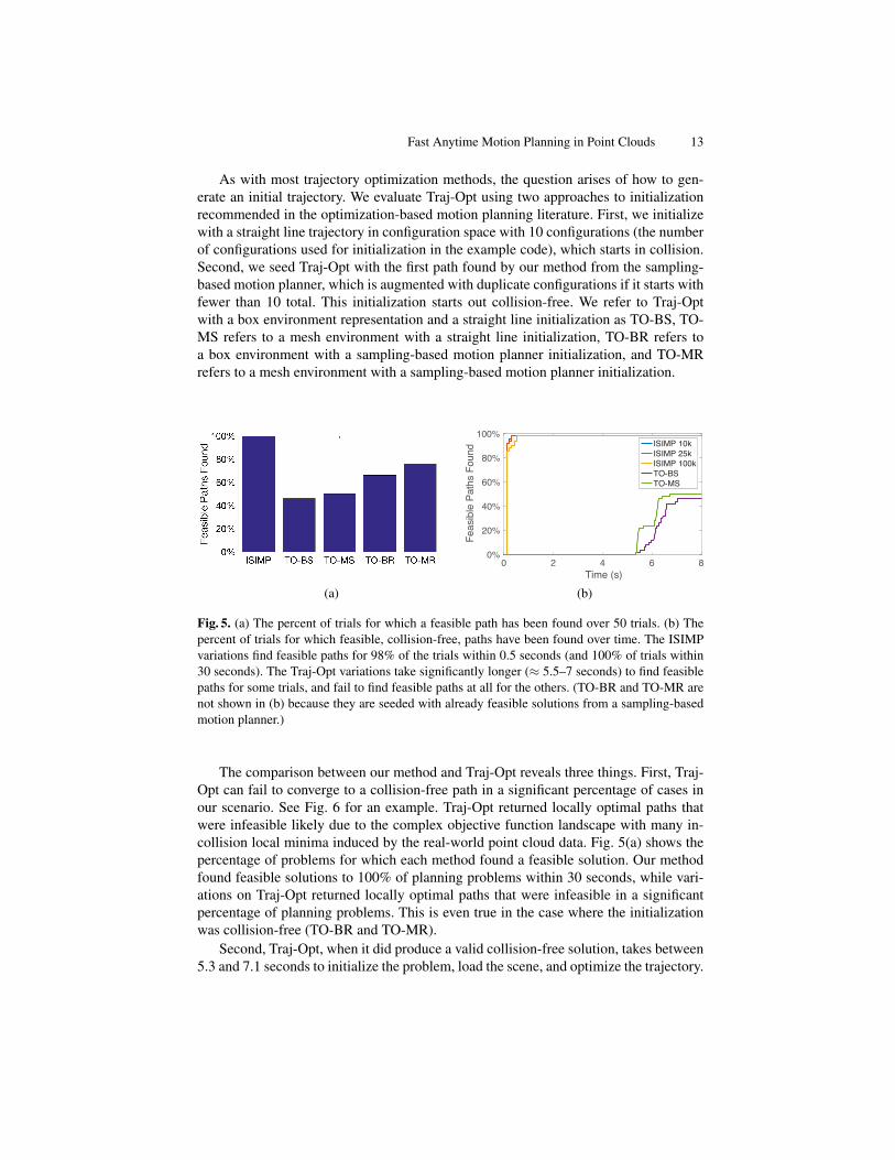
As with most trajectory optimization methods, the question arises of how to gen-erate an initial trajectory. We evaluate Traj-Opt using two approaches to initializationrecommended in the optimization-based motion planning literature. First, we initializewith a straight line trajectory in configuration space with 10 configurations (the numberof configurations used for initialization in the example code), which starts in collision.Second, we seed Traj-Opt with the first path found by our method from the sampling-based motion planner, which is augmented with duplicate configurations if it starts withfewer than 10 total. This initialization starts out collision-free. We refer to Traj-Optwith a box environment representation and a straight line initialization as TO-BS, TO-MS refers to a mesh environment with a straight line initialization, TO-BR refers toa box environment with a sampling-based motion planner initialization, and TO-MRrefers to a mesh environment with a sampling-based motion planner initialization.

(a)

0 2 4 6 8Time (s)

0%

20%

40%

60%

80%

100%

Feas

ible

Pat

hs F

ound

ISIMP 10kISIMP 25kISIMP 100kTO-BSTO-MS

(b)

Fig. 5. (a) The percent of trials for which a feasible path has been found over 50 trials. (b) Thepercent of trials for which feasible, collision-free, paths have been found over time. The ISIMPvariations find feasible paths for 98% of the trials within 0.5 seconds (and 100% of trials within30 seconds). The Traj-Opt variations take significantly longer (≈ 5.5–7 seconds) to find feasiblepaths for some trials, and fail to find feasible paths at all for the others. (TO-BR and TO-MR arenot shown in (b) because they are seeded with already feasible solutions from a sampling-basedmotion planner.)

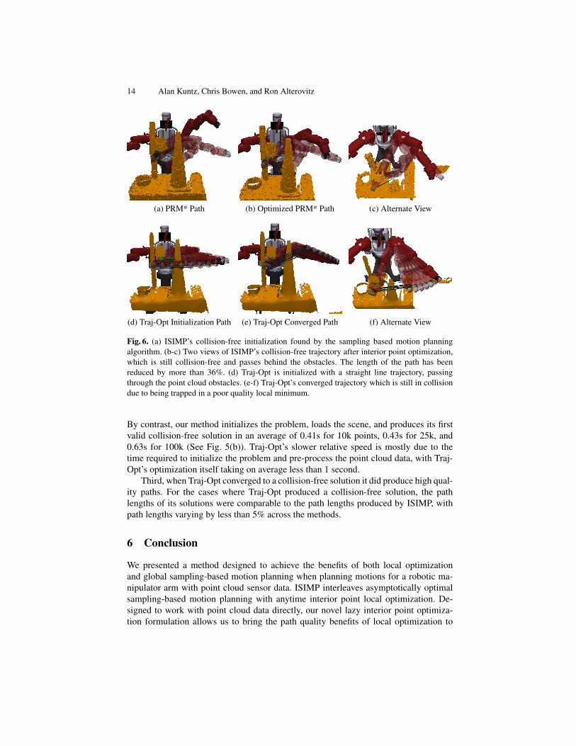
The comparison between our method and Traj-Opt reveals three things. First, Traj-Opt can fail to converge to a collision-free path in a significant percentage of cases inour scenario. See Fig. 6 for an example. Traj-Opt returned locally optimal paths thatwere infeasible likely due to the complex objective function landscape with many in-collision local minima induced by the real-world point cloud data. Fig. 5(a) shows thepercentage of problems for which each method found a feasible solution. Our methodfound feasible solutions to 100% of planning problems within 30 seconds, while vari-ations on Traj-Opt returned locally optimal paths that were infeasible in a significantpercentage of planning problems. This is even true in the case where the initializationwas collision-free (TO-BR and TO-MR).

Second, Traj-Opt, when it did produce a valid collision-free solution, takes between5.3 and 7.1 seconds to initialize the problem, load the scene, and optimize the trajectory.


(a) PRM* Path (b) Optimized PRM* Path (c) Alternate View

(d) Traj-Opt Initialization Path (e) Traj-Opt Converged Path (f) Alternate View

Fig. 6. (a) ISIMP’s collision-free initialization found by the sampling based motion planningalgorithm. (b-c) Two views of ISIMP’s collision-free trajectory after interior point optimization,which is still collision-free and passes behind the obstacles. The length of the path has beenreduced by more than 36%. (d) Traj-Opt is initialized with a straight line trajectory, passingthrough the point cloud obstacles. (e-f) Traj-Opt’s converged trajectory which is still in collisiondue to being trapped in a poor quality local minimum.

By contrast, our method initializes the problem, loads the scene, and produces its firstvalid collision-free solution in an average of 0.41s for 10k points, 0.43s for 25k, and0.63s for 100k (See Fig. 5(b)). Traj-Opt’s slower relative speed is mostly due to thetime required to initialize the problem and pre-process the point cloud data, with Traj-Opt’s optimization itself taking on average less than 1 second.

Third, when Traj-Opt converged to a collision-free solution it did produce high qual-ity paths. For the cases where Traj-Opt produced a collision-free solution, the pathlengths of its solutions were comparable to the path lengths produced by ISIMP, withpath lengths varying by less than 5% across the methods.

6 Conclusion

We presented a method designed to achieve the benefits of both local optimizationand global sampling-based motion planning when planning motions for a robotic ma-nipulator arm with point cloud sensor data. ISIMP interleaves asymptotically optimalsampling-based motion planning with anytime interior point local optimization. De-signed to work with point cloud data directly, our novel lazy interior point optimiza-tion formulation allows us to bring the path quality benefits of local optimization to


the anytime performance of sampling-based methods, while providing completenessand global asymptotic optimality guarantees not present in current optimization-basedmotion planning methods. The results demonstrate that our method, which combinesinterior-point optimization and asymptotically optimal sampling-based motion plan-ning, outperforms asymptotically optimal sampling-based motion planning alone, pro-ducing higher quality motion plans earlier. Our method outperforms an optimization-based method, Traj-Opt, in the percentage of collision-free solutions found and in thetime to the first valid solution.

In the future, we plan to evaluate ISIMP on other robotic systems of varying di-mensionality to further assess its efficacy. We also intend to incorporate more complexconstraints, such as task constraints, into the method and to explore other optimizationobjectives, such as clearance from obstacles. Additionally, we will investigate the inter-esting question of how to best balance the time spent on sampling versus optimizing.

Acknowledgments

This research was supported in part by the U.S. National Science Foundation (NSF)under awards CCF-1533844 and IIS-1149965 and the U.S. National Institutes of Health(NIH) under award R01EB024864.

References

1. Arslan, O., Tsiotras, P.: Use of relaxation methods in sampling-based algorithms for optimalmotion planning. In: Proc. IEEE Int. Conf. on Robotics and Automation (ICRA). pp. 2421–2428 (May 2013)

2. Berenson, D., Simeon, T., Srinivasa, S.S.: Addressing cost-space chasms in manipulationplanning. In: Proc. IEEE Int. Conf. Robotics and Automation (ICRA). pp. 4561–4568 (May2011)

3. Carriker, W., Khosla, P., Krogh, B.: The use of simulated annealing to solve the mobilemanipulator path planning problem. In: Proc. IEEE Int. Conf. Robotics and Automation(ICRA). pp. 204–209 (May 1990)

4. Choudhury, S., Gammell, J.D., Barfoot, T.D., Srinivasa, S.S., Scherer, S.: Regionally acceler-ated batch informed trees (RABIT*): A framework to integrate local information into optimalpath planning. In: Proc. IEEE Int. Conf. Robotics and Automation (ICRA). pp. 4207–4214.Stockholm, Sweden (May 2016)

5. Sucan, I.A., Moll, M., Kavraki, L.E.: The open motion planning library. IEEE Robotics andAutomation Magazine 19(4), 72–82 (Dec 2012), http://ompl.kavrakilab.org

6. Denny, J., Amato, N.M.: Toggle PRM: Simultaneous mapping of C-free and C-obstacle - astudy in 2D. In: Proc. IEEE/RSJ Int. Conf. on Intelligent Robots and Systems (IROS). pp.2632–2639 (Sept 2011)

7. Dobson, A., Bekris, K.E.: Sparse roadmap spanners for asymptotically near-optimal motionplanning. Int. J. Robotics Research 33(1), 18–47 (2014)

8. Geraerts, R., Overmars, M.H.: Creating high-quality paths for motion planning. Int. J.Robotics Research 26(8), 845–863 (2007)

9. Hauser, K.: Lazy collision checking in asymptotically-optimal motion planning. In: Proc.IEEE Int. Conf. on Robotics and Automation (ICRA). pp. 2951–2957 (May 2015)


10. Janson, L., Schmerling, E., Clark, A., Pavone, M.: Fast marching trees: a fast marchingsampling-based method for optimal motion planning in many dimensions. Int. J. RoboticsResearch 34(7), 883–921 (2015)

11. Kalakrishnan, M., Chitta, S., Theodorou, E., Pastor, P., Schaal, S.: STOMP: Stochastic tra-jectory optimization for motion planning. In: Proc. IEEE Int. Conf. Robotics and Automation(ICRA). pp. 4569–4574 (May 2011)

12. Karaman, S., Frazzoli, E.: Sampling-based algorithms for optimal motion planning. Int. J.Robotics Research 30(7), 846–894 (Jun 2011)

13. Kavraki, L.E., Svestka, P., Latombe, J.C., Overmars, M.: Probabilistic roadmaps for pathplanning in high dimensional configuration spaces. IEEE Trans. Robotics and Automation12(4), 566–580 (Aug 1996)

14. Kobilarov, M.: Cross-entropy motion planning. Int. J. Robotics Research 31(7), 855–871(Jun 2012)

15. Kurniawati, H., Hsu, D.: Workspace importance sampling for probabilistic roadmap plan-ning. In: Proc. IEEE/RSJ Int. Conf. on Intelligent Robots and Systems (IROS). vol. 2, pp.1618–1623. IEEE (Sept 2004)

16. LaValle, S.M., Kuffner, J.J.: Randomized kinodynamic planning. Int. J. Robotics Research20(5), 378–400 (May 2001)

17. Li, L., Long, X., Gennert, M.A.: BiRRTOpt: A combined sampling and optimizing mo-tion planner for humanoid robots. In: IEEE-RAS 16th Int. Conf. on Humanoid Robots (Hu-manoids). pp. 469–476 (Nov 2016)

18. Luna, R., Sucan, I.A., Moll, M., Kavraki, L.E.: Anytime solution optimization for sampling-based motion planning. In: Proc. IEEE Int. Conf. Robotics and Automation (ICRA). pp.5068–5074 (May 2013)

19. Pan, J., Chitta, S., Manocha, D.: FCL: A general purpose library for collision and proximityqueries. In: Proc. IEEE Int. Conf. Robotics and Automation (ICRA). pp. 3859–3866 (May2012)

20. Park, C., Pan, J., Manocha, D.: ITOMP: Incremental trajectory optimization for real-timereplanning in dynamic environments. In: Int. Conf. Automated Planning and Scheduling(ICAPS) (2012)

21. Ratliff, N.D., Zucker, M., Bagnell, J.A., Srinivasa, S.: CHOMP: Gradient optimization tech-niques for efficient motion planning. In: Proc. IEEE Int. Conf. Robotics and Automation(ICRA). pp. 489–494 (May 2009)

22. Salzman, O., Halperin, D.: Asymptotically near-optimal RRT for fast, high-quality motionplanning. IEEE Trans. on Robotics 32(3), 473–483 (June 2016)

23. Schulman, J., Ho, J., Lee, A., Awwal, I., Bradlow, H., Abbeel, P.: Finding locally optimal,collision-free trajectories with sequential convex optimization. In: Robotics: Science andSystems (RSS). vol. 9, pp. 1–10 (Jun 2013)

24. Wachter, A., Biegler, L.T.: On the implementation of an interior-point filter line-search al-gorithm for large-scale nonlinear programming. Mathematical Programming 106(1), 25–57(2006)

25. Wright, S., Nocedal, J.: Numerical Optimization. Springer Science (1999)

Documents

Fast Anytime Motion Planning in Point Clouds by