Fast and Accurate NN Approach for Multi-Event Annotation of Time Series

Brijesh Garabadu Cindi Thompson Gary Lindstrom

School of Computing University of Utah

{garabadu, cindi, gary} @cs.utah.edu

Joe Klewicki

Mechanical Engineering Department University of Utah

klewicki@mech.utah.edu

Abstract Similarity search in time-series subsequences is an important time series data mining task. Searching in time series subsequences for matches for a set of shapes is an extension of this task and is equally important. In this work we propose a simple but efficient approach for finding matches for a group of shapes or events in a given time series using a Nearest Neighbor approach. We provide various improvements of this approach including one using the GNAT data structure. We also propose a technique for finding similar shapes of widely varying temporal width. Both of these techniques for primitive shape matching allow us to more accurately and efficiently form an event representation of a time-series, leading in turn to finding complex events which are composites of primitive events. We demonstrate the robustness of our approaches in detecting complex shapes even in the presence of “don’t care” symbols. We evaluate the success of our approach in detecting both primitive and complex shapes using a data set from the Fluid Dynamics domain. We also show a speedup of up to 5 times over a naïve nearest neighbor approach. Keywords Time Series Data Mining, Subsequence Matching, Querying Shapes, Nearest Neighbor, Pattern Matching, Clustering 1. INTRODUCTION Time Series data occur frequently in many scientific and business applications. Time series are one of the most frequently examined type of data by the data mining community. The problem of finding patterns and associating patterns for temporal rule discovery is an important research area in time series data mining. Due to the complex nature of the time series data, detailed study is not practical particularly with high volume data [23]. Reducing a high-dimension time series into a representation that is more easily understandable by the users is necessary and helpful in interpreting sections of a given time-series. Before we discuss the details of such

user defined shapes or events and their matches in a time series, we give a graphic example of shapes or events to help develop an intuition of the problem. Figure 1 shows various types of events occurring in a small portion of a time series.

Figure1: Example of different types of shapes or events occurring in a time series. The event representation of a time series can be used for different purposes as discussed in [8], some of which are as follows: (a) Association rule mining [4] in time series, which requires an event representation of time series. Events in our case are analogous to the primitive shapes in [9] for rule discovery in time series and frequent patterns in [18]. (b) Anomaly detection in time series uses a set of typical shapes to model normal behavior and detect future patterns dissimilar to known typical events or shapes [10]. (c) Finding approximate periodic patterns in occurrences of events in time series as discussed in [30]. (d) Hypothesis Generation as discussed in [11]. There has been a lot of work on efficiently detecting a particular shape in a time series [1, 3, 7, 12, 13, 16, 17, 22]. This is similar to querying the database for a particular shape. Our problem, however, is finding matches for a given set of shapes in any given time series. This problem can be seen as a simple extension of the earlier one. Figure 2 gives an intuition of the two problems. In this paper we demonstrate that using 1-NN (i.e. One Nearest Neighbor) along with single shape search techniques can actually get us high quality approximate matches in a reasonable amount of time. We

1

Figure 2: The problem of single shape search (left) and multiple shape searches (right) where qi is a query shape. provide various improvements of the simple approach to achieve considerable performance gain in terms of search time. One of the performance improvement techniques uses statistics of patterns/shapes collected from a small portion of a time series and uses this in early termination of distance calculation. We also used the GNAT (Geometric Near-Neighbor Access Tree) data structure as discussed in [5] to form a hierarchical tree to reduce the search space for the nearest shape. We show in the experiments that a speed up of up to 5 times is obtained depending on the width of subsequences searched. The second problem that we are trying to deal with is as follows: find all similar shapes of widely varying temporal widths. By widely varying we mean in the range of .50 times to ~5.0 times the width of the query templates, sometimes even more. Examples of such matches can be best demonstrated visually as shown in Figure 4. Dynamic Time Warping [6] can be used to detect shapes that are compressed or stretched along the time axis. But one of the common problems with this technique is that it cannot find the boundary (start and end points of a match) correctly. And even if some improvement of the simple DTW can detect boundaries correctly, the width of subsequences in which such searches can be performed is limited. This is as shown in Figure 3 where Dynamic Time Warping can find matches but not the correct shape boundary. Detecting correct boundaries for such shapes of widely varying width is important for two reasons: firstly, they are informative in the sense that users might want to see if at any particular point of time a particular event is happening or is already over; secondly, while using association rule mining for temporal rule discovery in multiple time series as in [9] and using parallel episode rule as in [28] when we are trying to correlate events across multiple time series, it is important to know at any particular time if events in two different time-series are overlapping each other or one is happening before the other, etc. Example rules as mentioned in [28] are “A overlaps B” or “A after B”. This problem is also very important for the dataset under consideration for one more reason: two different time series for the same attribute collected under different conditions or at two different locations in space have similar events compressed or stretched over time. It has been proven theoretically that such situations are common in the current domain (and dataset) and that the average ratio of the width of events

in two time series of the same attributes can be calculated using domain knowledge (see section 6.1 for more information).

1 2 3 4 5 6 7 8 9 10

q1

1 2 3 4 5 6 7 8 9 10

q1 q2 q3 q4

Figure 3: Match for a given query shape. Query template width is 25. The right window shows a match of window width=25 found using DTW. The actual boundary of the match is shown by the start and end arrows and the correct window size of the match should be 17 instead of 25. Motivation for using NN: Time series data is very high-dimensional. Nearest neighbor techniques have been shown to perform very well in low dimensional space. But with the increase in dimensionality, the scalability of the algorithm is the major problem [5]. However, we use 1-NN technique to search for only the primitive shapes (or simplest of shapes) and so the length of our subsequence is going to be very small in comparison to that of the whole time sequence. But this does not mean that we do not search for complex shapes. Complex shapes can be formed by combining one or more types of primitive shapes as discussed in [9]. An example of complex shape is “rapid transition from increasing to decreasing pattern” which can be represented as a combination of upward spike followed by a reverse spike or vice-versa. Various techniques have been developed in the past to accommodate “don’t care” symbols. The robustness of our technique lies in the fact that we can take care of “don’t care” symbols in complex shapes using a fairly simple technique (see section 5). The second motivation for using NN search for finding shapes lies in the typical requirement to distinguish between similar shapes of different amplitudes. An example is a search for different kinds of upward spikes (e.g. short, medium and tall spikes). This is a common requirement in many applications and is also found in many data sets from fluid dynamics domain. A major problem with such requirements is that we cannot do a general window based normalization as this would fit most of the subsequences into the same height, and distinguishing them based on their amplitude would no longer be possible. A straightforward solution is to normalize the windows into different heights. But given the number of possibilities of heights and the number of

Query Shape Matched Subsequence

End Point

Start Point

2

Figure: 4 Pattern matching for reverse spikes. The template pattern is of width 15. The matches are shown with the green boxes that indicate the width of the pattern. Note that patterns occur in various widths (in this case ranging from .800 to 2.733 times the width of the template pattern). different normalization ranges, this is not reasonable. Hence the need for a technique that can overcome this problem automatically by comparing the current window with various available shapes of different heights before labeling a subsequence as a match. Our contributions in this paper are twofold. Firstly, we use a nearest neighbor technique to attend the problem of finding matches for a given set of query shapes or events from a given time series and provide techniques for improvement of the search time. Secondly, we propose a technique to accurately detect boundary of similar shapes (or events) of widely varying temporal widths. In this section we motivated a problem and an approach that we propose to use to handle such problems. The rest of the paper is organized as follows. In section 2 we define the problem of event matching formally along with the definition of some of the terms that we are going to use throughout the paper. In section 3 we discuss the approach using 1-NN to handle the problem elegantly and also discuss improvement techniques for a significant reduction in computational time. In section 4 we provide an algorithm for searching patterns of widely varying temporal widths. Section 5 discusses the technique of finding complex patterns using simple shapes. Section 6 provides experiments for extensively evaluating the accuracy of our approach and comparing various improvements for speedup. In section 7 we briefly discuss related work in time series data mining and particularly the subsequence matching techniques. Section 8 provides a conclusion followed by possible future directions to our work. 2. DEFINITIONS AND NOTATIONS Here we define a few terms that are of importance to this paper. Definition-1 Time Series: A time series T = {t1, t2,…, tn} is a set of ordered real-valued variables.

Definition-2 Subsequence: A subsequence ssi is a small section of a time series that consists of values from contiguous positions in the time series. If m is the length of the subsequence then in our case m << n where n is the length of the time series. SS = {ss1, …, ssn-m+1} is the set of all consecutive subsequences in a given time series. Definition-3(a) Window: A window of length m is a subsequence of length m from the time series T. Sliding window technique is used to retrieve all consecutive windows from a time series. Definition-3(b) Shape: A shape is an ordered, consecutive, real-valued vector representing a particular subsequence of interest in a time series. An event can be represented with a shape. In the rest of the paper we will use shape, event and pattern interchangeably. Definition-4 Match: Given a time series T, a shape s, a positive threshold t and a subsequence c starting at position q in the time series, if Dist(s,c) ≤ t, then c is called a matching subsequence for s. Dist(s,c) is the distance function to calculate the distance between two real-valued vectors. Euclidean distance and DTW are examples of distance functions. Definition-5 Best Match and Trivial Match: Given a time series T, a shape s and a threshold t there can be a set of consecutive subsequences C={ci, ci+1, …, ci+m} where subsequence ci starts at the ith position in the time series and all of them are a matches. The best match is the one subsequence that is least distant from s i.e. BestMatch(C)=ck where Dist(s, ck)= minj=i:i+m (Dist(s, cj)). All the remaining matches in C are trivial matches. The definition of trivial match is similar to that in [8] in some ways. This is demonstrated in Figure 5.

vωz

3

Figure 5: Trivial Matches. From [8] Definition-6 Single Shape Search: Given a shape s of a given width w, a threshold t and a time-series T, find all non-trivial matches in all the subsequences of width w in T. Definition-7 Multiple Shape Search: Given a set of shapes/patterns S = {s1, s2 ... sn} of a given width w, a threshold t and a time-series T, find all the Best Matches for shapes in S. The matches should be non-overlapping. Definition-8 Single Shape Matches of Widely Varying Widths: Definition-8(a) Different but constant width match: Given a shape s of width w, a threshold t and a time-series T, find all the Best Matches of width w’ in T where w’ = w + τ and τ is some constant value. Definition-8(b) Different range of widths match: Given a shape s of width w, a range of thresholds Rt and a time-series T, find all the Best Matches of width w’ in T where w’ is any width within the range w ± τ time units. This is different from Definition-8(a) in the sense that 8(a) finds all matches with one particular window width w’ while 8(b) deals with searching for all matches with a window width in the range of w ± τ. Definition 9: Multiple Shape Matches of Widely Varying widths: Same as in definition-8 except here the search is for more than one shape. One of the goals of this paper is Multiple Shape Search and Multiple Shape Matches of Widely varying widths. 3. NEAREST NEIGHBOR APPROACH In this section we discuss the NN approach for dealing with the problems defined in definitions 7 through 9 of the previous section. But before that we will see how shapes can be discovered from time series using clustering. These shapes in addition to other user defined templates are later used as the set of query shapes for NN search. 3.1. Clustering to extract shapes from time series: Clustering is used to group similar objects together. It has been used to discover distinct shapes from time-series, which in turn can be used for symbolic representation of time-series as in [9]. Such symbolic representations are

used for temporal rule discovery as shown in the above work. We use clustering to obtain distinct and maximally different shapes from a small portion of a time series. The users label these subsequences as “interesting” or “non-interesting”. The users can add their own shapes or templates to the clustering results and label them as “interesting”. Hence the result of clustering, and the extra “interesting” shapes, form the set of shapes S while Q is the subset of S that are labeled as “interesting” by the user. We explored two types of clustering: k-means and hierarchical clustering and finally decided to use k-means for our purpose since we are looking for mostly simple and primitive subsequences. 3.2. 1-NN for parallel search of multiple shapes: Nearest Neighbor in the subsequence search problem can be defined as follows: given a set of subsequences SS and a query shape q, find all the non-trivial matches in SS that are within a distance r from q. SS is the set of subsequences in time series T obtained using sliding window of width w and sliding distance d. The 1-NN search is the problem of finding the closest match to q from SS. If the search is for multiple shapes, then search for each of these shapes individually, by scanning through S once for every shape. Our use of 1-NN is slightly different from the above technique. Unlike the above approach, we take each subsequence ssi in SS and find if there is a match to one of the shapes in Q and also satisfy some constraints. And we perform all the required matching in just one sequential scan through SS as opposed to multiple scans of the earlier approach. The constraints can be in the form of a distance threshold or a correlation coefficient threshold.

Algorithm 1: 1NNP (1NN Parallel)

1NNP (T, Q, w, threshold) 1. Use sliding window to retrieve one subsequence

(window of width=w) at a time from the time series.

2. Do the following for each of the above subsequences: o Find the closest shape in the set of shapes Q.

Euclidean distance measure is used for this purpose.

o Label the subsequence with the closest shape.

3. Remove trivial matches. 4. Prune all matches below a specified threshold.

4

Given a set of shapes Q of width w and a time series T, we use the following simple algorithm, we call 1NNP (1NN Parallel), to find all non-trivial matches in T.

Removing trivial matches: The algorithm for removing all trivial matches is as follows: For each of the shapes in Q, do the following: a) Find all the matches for the current shape from the

list of ordered matches obtained in Step (2) above. b) For each set of consecutive matches in the above list,

find the match that is least distant from the current shape.

Consecutive matches in (a) refer to all matches with consecutive offsets. We can remove trivial matches efficiently by keeping track of the distance measure for each match in Step (2) of Algorithm 1. Pruning of matches: Pruning as mentioned in Step (4) of Algorithm 1 is done using a correlation coefficient threshold. This is the constraint applied on individual matches. Correlation Coefficient (CC) threshold can be used for shapes that are fairly simple. The correlation coefficient can be maintained at a fixed value for all the shapes. This prevents the need to find a good distance threshold for each query shapes. We show experimentally that this threshold actually yields good results in terms of accuracy of matches. Our system can accommodate any distance metric including both Euclidean Distance (ED) as well as Dynamic Time Warping (DTW) for pruning. DTW is computationally expensive but is more accurate to matches with various levels of elasticity along the time axis (CC threshold won’t work well). We show the ED can give us really good results when the primitive shapes are fairly simple. DTW can be used to find shapes deformed along the time axis. We call the above algorithm 1NN Parallel because it uses 1NN search and it can find matches for all the shapes in Q in parallel with a single sequential scan. This is unlike the naive approach where search for each shape requires a sequential scan through all the subsequences in time series T. One of the obvious problems with our approach is the high number of distance calculations that need to be performed. One simple technique to speed up algorithm is by using the “early termination” technique in distance measurement. This helps in Step 2(a) of the 1NNP algorithm which has been seen to take 99% of the computation time. We call this improved algorithm the 1NNP_ETD (1NNP with Early Termination in Distance computation). The “early termination” for distance calculation algorithm for our purpose is as follows:

// finding closest shape using the early termination // distance calculation // ssi → current subsequence and Q → set of shapes closest_shape(Q, ssi) 1. best_query=1 2. best_distance = dist(ssi, q1) 3. For each shape qj in Q, do the following:

a. curr_distance = dist_et(si, qj, best_distance) b. if (curr_distance < best_distance) best_distance = curr_distance best_query = qj

// early termination distance calculation dist_et (s, q, best_distance) sum=0; 1. for i=1:n 2. sum+= (s[i]-q[i])^2 // Euclidean Distance 3. if (sum >= best_distance) 4. return sum 5. end 6. end Figure 6 shows graphically how early termination works. It can be seen in the experiment section that using the early termination distance calculation efficiently reduces the computation time by almost one-third the original time of 1NNP. Shapes in Q are matched in the order in which they appear in the list. Since early termination is dependent on how early we find the closest match, the idea is to order the shapes for most efficient use of early termination. We use the statistics gathered during clustering to decide the order of the search to improve the classifier performance. Table 2 shows the result of k-means clustering with k=10. The number of windows and the percentage of windows covered by each of the 10 shapes are shown in the table. It can be seen that just the 3 most frequent shapes account for 70% of the subsequences and 5 most frequent shapes account for 90% of the subsequences. It is also interesting to note that the “interesting” shapes identified by the users are # 6 and # 9 which account for 2% of the matches. Also the “extra” templates added by the users are of similar rarity. Given all these statistics, it can be inferred that more than 95% of the subsequences to be searched are going to be unsuccessful matches. In other words only less than 5% of the searches are going to be matches. Given all these statistics, the question is can we order the shapes so that the early termination of distance calculation is most efficient. Early termination is most successful when the least distant shape is matched first during the matching process. In such a case, matching with the rest of the query shapes will result in efficient early termination of the distance calculation as shown in Figure 6.

5

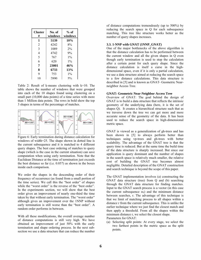
Table 2: Result of k-means clustering with k=10. The table shows the number of windows that were grouped into each of the 10 shapes found using clustering on a small part (10,000 data points) of a time series with more than 1 Million data points. The rows in bold show the top 3 shapes in terms of the percentage of matches.

Figure 6: Early termination during distance calculation for windows of width=25. The shape shown in dotted line is the current subsequence and it is matched to 4 different query shapes. The best case ordering of matches to query shape (which is the case in the current situation) can save computation when using early termination. Note that the Euclidean Distance at the time of termination just exceeds the best distance so far (i.e. 0.057) as shown in the boxes inside each comparison. We order the shapes in the descending order of their frequency of occurrence (as found from a small portion of the time series). We call this the “best order” of shapes while the “worst order” is the reverse of the “best order”. In the experiments section, we will show that the best order gives an improvement of nearly one-third the time taken by that without early termination. The “worst order” although gives an improvement over the 1NNP without early termination is still worse than the “best order”. A random order performs in between. With all these modifications, the overall average number of distance computations is still very high. We have obtained an improvement of just 50% with the early termination and shape ordering process. In the next sub-section we use a data structure that can reduce the number

of distance computations tremendously (up to 500%) by reducing the search space in Q for each subsequence matching. This tree like structure works better as the number of query shapes increases. 3.3. 1-NNP with GNAT (1NNP_GNAT) One of the major bottlenecks of the above algorithm is that the distance calculation has to be performed between the current window and all the given shapes in Q even though early termination is used to stop the calculation after a certain point for each query shape. Since the distance calculation is itself a curse in the high-dimensional space, even if it is only a partial calculation, we use a data structure aimed at reducing the search space to a few distance calculations. This data structure is described in [5] and is known as GNAT- Geometric Near-neighbor Access Tree. GNAT: Geometric Near-Neighbor Access Tree Overview of GNAT: The goal behind the design of GNAT is to build a data structure that reflects the intrinsic geometry of the underlying data (here, it is the set of shapes Q). It creates a hierarchical structure such that as we traverse down the tree we can get more and more accurate sense of the geometry of the data. It has been used to reduce the search space in high-dimensional metric space. GNAT is viewed as a generalization of gh-trees and has been shown in [5] to always perform better than techniques using vp-trees and gh-trees with better scalability. The advantage of the GNAT tree is that the query time is reduced. But at the same time the build time of the data structure is sharply increased. But since our application is query dominant and the number of shapes in the search space is relatively much smaller, the relative cost of building the GNAT tree becomes almost negligible. Detailed description of the GNAT construction and search technique is beyond the scope of this paper. The GNAT implementation involves (a) constructing the GNAT data structure (tree) from Q and (b) searching through the GNAT data structure for finding matches. Input to the GNAT search process is a vector (in this case the current subsequence ssi) and the minimum distance between searches, r. The advantage of this technique is that we limit of matching process to all shapes within a distance r from the current subsequence. This is unlike the earlier technique where we just find the closest match and then apply a threshold. From all the shapes within the minimum distance r, we select the closest shape. Parameters for GNAT: (a) Selecting split points: At every stage, we select the

two farthest points in the metric space as the split points.

Cluster #

No. of windows

% of windows

1 5139 10% 2 4242 8% 3 1089 2% 4 4742 9% 5 767 1% 6 620 1% 7 23001 46% 8 6733 13% 9 753 1%

10 2890 5%

6

(b) Degree of a node: We choose a maximum degree of 2 for each node in the tree.

1NNP_GNAT Algorithm:

Algorithm 2: 1NNP_GNAT

Early termination in the distance calculation cannot be used with GNAT. However, we can take advantage of the high frequency of the most frequent shape in Q and stop with searching in GNAT tree if the following condition is satisfied:

Dist (ssi, f) < (½ * Dist (f , fc)) where, ssi = current subsequence, f is the most frequent shape in Q and fc is the closest shape to f in Q. This will ensure that f is the closest shape to ssi in Q because of the triangle inequality condition satisfied by Dist() functions like Euclidean Distance, etc. This condition is checked for just before Step (3) in algorithm 2. If satisfied, the closest shape returned is f. We call this algorithm 1NNP_GNAT_EFSP (EFSP for Early Frequent Shape Pruning). 4. FILTER BASED GRADIENT SEARCH In the previous section we discussed the problem of searching a time series for a given set of query shapes and have used various techniques to speed up the basic 1-NN search algorithm. In this section we propose an algorithm that is used to find similar shapes of widely varying temporal widths as shown in Section 1. We use the fast 1NN from section 3 to speed up the search process. We also describe a novel scaling technique for scaling a query shape in the time axis before finding matches. We propose a technique we call Filter Based Gradient Pattern Matching to solve the problem of widely varying temporal width. Filter Based Gradient Pattern Matching (FBGPM) is based on a technique whereby we use multiple versions of the same query shape and search for

matches for each versions of the shape. Each version of the shape is of a different temporal width: stretched or compressed along the time axis. The technique is called “gradient” because we use a gradient of widths for the same pattern. The gradient is formed by selecting a range of compression and stretching levels. We call it a “filter based” approach since for each scaled version of the shape/ pattern we find matches from the time series and remove or filter out all the matched windows from the time series before performing matching with the next version of the shape. The algorithm for implementing the FBGPM technique is as follows:

Algorithm 3: FBGPM

GS (Gradient Scale): A range of scaling percentages by which a shape is to be scaled before searching for matches. GT (Gradient Threshold): A set of thresholds for deciding a good match for each version of shapes decided by GS. The algorithm works as follows: We form a set of subsequences which initially is just one subsequence that represents that entire time series <1, length(T)>. For each of the scale in the gradient, the shapes in Q are scaled to the temporal scale using a Hinge Based Scaling technique described below. Q’ is a scaled version of Q. The 1NN algorithm described in Section 4 is used to find all the matches for shapes in Q’. The matches are filtered out from the current set of subsequences and a new set of subsequences is formed. For example initially we have a subsequence {<1, 200>} in the set of subsequences where 200 is the length of the time series. Let’s say we found two matches with offset 21 and 106 and the current width of shapes in Q’ be w’=30. After filtering, the new set of subsequences is {<1, 20>, <51, 105>, <136, 200>}. This process of scaling of shapes in Q, finding matches in the

1NNP_GNAT (T, Q, w, threshold, r) Input: Output: 1. Construct the GNAT tree from Q 2. Use sliding window to retrieve one subsequence

(window of width=w) at a time from the time series.

3. Do the following with each of the above subsequences obtained in (2):

a. Find the closest shapes in the set of shapes Q using the GNAT search that are within a distance r. Euclidean distance measure is used for this purpose.

b. Label the subsequence with the closest shape from (a).

4. Remove redundant matches. 5. Prune all matches below a specified threshold.

FBGPM (T, Q, w, GS, GT) 1. Subs = {<1,length(T)>} //initial set of subsequences 2. Select a scale gsi from the gradient scale in GS. 3. w’ = w + (w*gsi/100) // scaled width of patterns 4. Scale all the shapes in Q to the current temporal

scale gsi using HingeBasedScaling. This is done as follows:

Q’ = HBS(Q, w, gsi) 5. c_threshold = GT(i) // current threshold 6. Apply 1NN search algorithm to find all matches

for the shapes in Q’. c_ms = 1NN_Parallel(T, Q’, w’, c_threshold) 7. Filter the matched window in c_ms and form a

new set of subsequences. Subs = Filter(T, c_ms, w’) 8. Repeat steps (2-7) for each of the scales in GS in

the given order..

7

set of subsequences followed by filtering of matches is continued for each of the scales in the gradient. Parameters for FBGPM: There are some choices that we have to make when using the above algorithm. They are as follows: 1. Choice of the gradient. (a) Order of gradient: A gradient can begin with the most compressed pattern and gradually move towards the original patterns ending up with the most stretched pattern. We will call this gradient COS (Compressed->Original->Stretched). Another possible gradient can be the opposite of the above gradient where we start with the most stretched version of patterns in Q and end up with the most compressed versions. We will call this SOC (Stretched->Original->Compressed). We will test with both versions of the gradient to find the better of the two. (b) Values of the gradient: We also need to decide the amount of stretching and compression that needs to be done. For example we can start with a compression level of 80% and go up in steps of 10% (i.e. -80%, -70%, ….., -10%, 0%, 10%, …, 80%). Or we can start with a compression of -75% and go up in steps of 25% up to a stretching of 75%. The compression and the stretching levels need not be symmetric. These choices have to be made based on the time series and the kind of pattern that we are looking for. For example, if most of the patterns occurring in the time series are thinner than the original pattern width, then it makes sense to have more compression levels than stretched levels in the gradient scale (GS). 2. Choice of thresholds for a given gradient. The two threshold choices are as follows: (a) Single threshold for all degrees of scaling. (b) Variable thresholds depending upon the scaling. A variable threshold with a very high initial value is suggested since we would want all the initial matches to be highly accurate so that the current version of the pattern doesn’t match the shapes that might match more accurately with a wider or thinner version of the pattern that occurs later on in the gradient. Hinge Based Scaling: A Pattern Scaling Technique In FBGPM, we form a gradient scale. Now we need a way to scale the pattern to a particular level of compression or stretching along the time axis as mentioned in Step (4) of the FBGPM algorithm. We propose a technique we call Hinge Based Scaling to perform scaling on the temporal axis. The idea behind hinge based scaling is to divide a shape into multiple segments. The segments are decided by the location of hinge points: the points at which there is a reversal in the trend in the shape (articulation points in a shape). This point is otherwise known as articulation point. The various segments are compressed or stretched individually

to a required width by insertion or removal of points using the averaging of two consecutive points technique. Each of the segments is then offset and amplitude scaled to match the offset and amplitude in the original shape. The individual segments are then merged at the hinge/articulation points to form the scaled pattern. An example of scaling Hinge Based scaling is shown in figure 7.

0

20

40

60

80

100

120

140

160

1 3 5 7 9 11 13 15 17 19 21 23 25

Original Normal 25% Hinge 25%

Original Pattern

25 % compressed with a Simple Scaling technique using consecutive point averaging with offset and amplitude scaling

25 % compressed using Hinge Based Technique

Figure 7: Hinge Based Scaling vs. Simple Temporal Scaling. With Hinge Based Scaling, the overall shape is more consistent with the original shape. Note that the left end of the HB Scaled shape matches the start point of the original shape. The start offset of Simple Scaled shape is raised above the original start point offset. 5. EVENT REPRESENTATION OF TIME

SERIES AND SEARCHING FOR COMPLEX EVENTS/SHAPES

An event representation of the time series is formed as mentioned in [9]. Matches for each of the shapes in the set of “interesting” events, Q, are found using the 1-NN algorithm. Similar shapes of widely varying width are found using the Filter Based Gradient Approach mentioned in Section 5. Our technique of event representation differs from [9] in that we do not match every window to a shape. Rather we just label each non-trivially matched window with the name of symbol of the event/shape. All the unmatched subsequences are labeled as “non-interesting” or “don’t cares”. This form of event representation is also similar to [18] where the time series is labeled with “increasing”, “decreasing” and “plateau”

8

labels. An example event representation of a time series is shown in figure 8.

gradient may then be decomposed in to the difference of two velocity –vorticity correlations, one of which is vωz. Thus, exploration of the coherent signatures in the vωz signals has direct relevance to the instantaneous

1 25 35 40 50 72 78 88 90 110 117 126Start offset of each match

1 25 35 40 50 72 78 88 90 110 117 126Start offset of each match

1 25 35 40 50 72 78 88 90 110 117 126Start offset of each match

1 25 35 40 50 72 78 88 90 110 117 126Start offset of each match

Figure 8: Event Representation of Time Series where the time series is replaced with the symbols for the primitive shapes. The 3 shapes matched here are P1, P2 and P3 and DC stands Don’t Care regions or the “uninteresting” regions. Primitive shapes are used for finding more complex shapes as described in [9]. An example of a complex shape is an “upward spike followed by a reverse spike” as shown in Figure 3. Such a search approach allows for “don’t care” symbols within complex shapes. Abstract patterns for finding such complex shapes can be formed as follows: [Rule-1: P1 → P2, τ] which can be interpreted as an event P1 followed by an event P2 with the maximum allowed gap being τ time units. Event representation is commonly used for temporal rule discovery as in [9]. Because of space limitations we are not going to discuss this part which is also beyond the scope of current paper. 6. EXPERIMENTS AND RESULTS 6.1 Dataset: To evaluate our approach, we use measurements from one of the signals collected from boundary layer experiments in the fluid dynamics research domain. This is the vωz signal which is collected at a frequency of 500Hz. We use the vωz time series from these experiments. The vωz signals are derived from four element hot-wire sensor measurements of the zero pressure gradient turbulent boundary layer as discussed in [24]. The four element sensor is unusual in that it allows the simultaneous measurement of the fluctuating axial and wall-normal velocities and the spanwise vorticity, and thus constitutes one of very few data sets that have directly measured vωz. Owing to the fact that the boundary layers studied developed over a 15m length at 25 different locations, an important characteristic of these experiments is their high spatial and temporal resolution. The motivations for studying coherent patterns in the vωz signals presented herein are primarily derived from the time averaged Navier-Stokes equations as applied to wall-bounded flows. In particular, it may be shown in [25] that the net effect of the turbulence on mean flow dynamics is reflected in the gradient of the Reynolds stress. This

mechanisms for momentum transport. DC P1 DC P2 DC P1 P3 P2 DC P1 P2 ………...24 10 5 10 22 6 5 10 20 7 9

Width of each match

DC P1 DC P2 DC P1 P3 P2 DC P1 P2 ………...24 10 5 10 22 6 5 10 20 7 9

Width of each match

DC P1 DC P2 DC P1 P3 P2 DC P1 P2 ………...24 10 5 10 22 6 5 10 20 7 9

Width of each match

24 10 5 10 22 6 5 10 20 7 9

Width of each match

6.2 Data Preprocessing Different time-series of the vωz attribute that are collected at different points in the boundary layer or under different experimental conditions have very different scales (both amplitude and temporal widths). The maximum value of amplitude varies widely between two time-series (e.g. 0.3 and 1000). To handle this problem, we normalized all the time series to a fixed range. The second problem with the data set is the widely varying temporal widths of events. This happens because of the acceleration or deceleration of the speed at which events occur in the time-series. Researchers can theoretically find the average width of events in the time-series of an attribute collected at different points in the boundary layer. We use this value to determine the base width of all the shapes in the query set Q. The actual width of patterns can range from anywhere between -75% to +200% of the base width. 6.3 Experiments We performed all our experiments using Euclidean distance. However for comparison of matches, we did us Dynamic Time Warping (DTW) in some of the experiments. ED is found to get us the desired results when the searched shape is not very complex. For complex primitive shapes that cannot be found using the event representation (discussed in section 5), DTW gives better accuracy. We conducted two types of experiments; the goals for each are as follows: (a) To compare the performance of the 1NN approaches in terms of computation time, and (b) To determine the accuracy of the FBGPM with 1NN algorithm in terms of finding patterns “correctly” and “accurately” (we will see the definitions below). 6.3.1. Comparison of Computation Time of 1NN approach: We use the results of our basic 1NNP algorithm as the baseline. Another baseline could be a sequential search algorithm that searches for one pattern at a time by sequentially scanning through the time series. For example if there are m shapes in the query set Q, this approach will require m sequential scanning of the time series. Obviously the number of distance computations of this approach will be the same as that of the basic 1NNP algorithm but the overhead in 1NNP is much less due to the single scan as opposed to the multiple scans in the serial approach. Thus the 1NNP is faster than the serial algorithm and hence a good baseline.

9

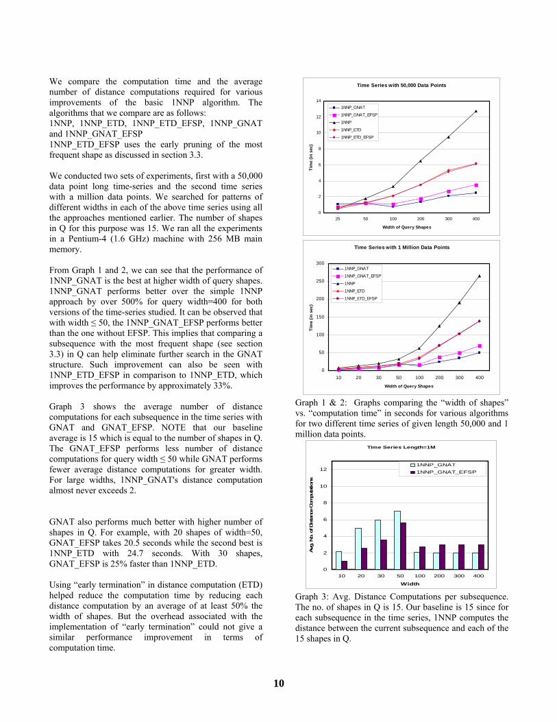
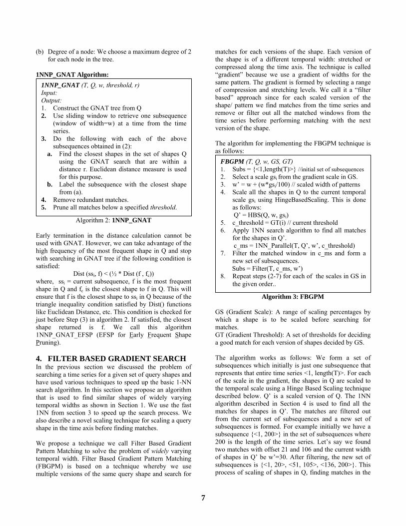
We compare the computation time and the average number of distance computations required for various improvements of the basic 1NNP algorithm. The algorithms that we compare are as follows: 1NNP, 1NNP_ETD, 1NNP_ETD_EFSP, 1NNP_GNAT and 1NNP_GNAT_EFSP 1NNP_ETD_EFSP uses the early pruning of the most frequent shape as discussed in section 3.3. We conducted two sets of experiments, first with a 50,000 data point long time-series and the second time series with a million data points. We searched for patterns of different widths in each of the above time series using all the approaches mentioned earlier. The number of shapes in Q for this purpose was 15. We ran all the experiments in a Pentium-4 (1.6 GHz) machine with 256 MB main memory. From Graph 1 and 2, we can see that the performance of 1NNP_GNAT is the best at higher width of query shapes. 1NNP_GNAT performs better over the simple 1NNP approach by over 500% for query width=400 for both versions of the time-series studied. It can be observed that with width ≤ 50, the 1NNP_GNAT_EFSP performs better than the one without EFSP. This implies that comparing a subsequence with the most frequent shape (see section 3.3) in Q can help eliminate further search in the GNAT structure. Such improvement can also be seen with 1NNP_ETD_EFSP in comparison to 1NNP_ETD, which improves the performance by approximately 33%. Graph 3 shows the average number of distance computations for each subsequence in the time series with GNAT and GNAT_EFSP. NOTE that our baseline average is 15 which is equal to the number of shapes in Q. The GNAT_EFSP performs less number of distance computations for query width ≤ 50 while GNAT performs fewer average distance computations for greater width. For large widths, 1NNP_GNAT's distance computation almost never exceeds 2. GNAT also performs much better with higher number of shapes in Q. For example, with 20 shapes of width=50, GNAT_EFSP takes 20.5 seconds while the second best is 1NNP_ETD with 24.7 seconds. With 30 shapes, GNAT_EFSP is 25% faster than 1NNP_ETD. Using “early termination” in distance computation (ETD) helped reduce the computation time by reducing each distance computation by an average of at least 50% the width of shapes. But the overhead associated with the implementation of “early termination” could not give a similar performance improvement in terms of computation time.

Time Series with 50,000 Data Points

0

2

4

6

8

10

12

14

25 50 100 200 300 400

Width of Query Shapes

Tim

e (in

sec

)

1NNP_GNAT

1NNP_GNAT_EFSP

1NNP

1NNP_ETD

1NNP_ETD_EFSP

Time Series with 1 Million Data Points

0

50

100

150

200

250

300

10 20 30 50 100 200 300 400

Width of Query Shapes

Tim

e (in

sec

)

1NNP_GNAT

1NNP_GNAT_EFSP

1NNP

1NNP_ETD

1NNP_ETD_EFSP

Graph 1 & 2: Graphs comparing the “width of shapes” vs. “computation time” in seconds for various algorithms for two different time series of given length 50,000 and 1 million data points.

Time Series Length=1M

0

2

4

6

8

10

12

10 20 30 50 100 200 300 400

Width

Avg

. No.

of D

ista

nce

Com

puta

tions

1NNP_GNAT1NNP_GNAT_EFSP

Graph 3: Avg. Distance Computations per subsequence. The no. of shapes in Q is 15. Our baseline is 15 since for each subsequence in the time series, 1NNP computes the distance between the current subsequence and each of the 15 shapes in Q.

10

6.3.2. FBGPM for shapes of widely varying width: We define a match to be correct if the classifier label for a window is same as that labeled by users. An accurate match is one whose end points are within ±δ data points from the end points of the window containing the actual match (as identified by users). Let so and eo be the start and end point of a window containing an event as labeled by users. Let sf and ef be the end points of the window found by our FBGPM technique. A match is considered accurate if |so-sf|= δ and |eo-ef|= δ. For our experiments, we set δ=3. We conducted experiments for FBGPM with various time series subsequences of length 10,000 data points and 50,000 data points. We used a SOC gradient of {+100%, +75%, +50%, +25%, 0%, -10%, -20%, -30%, -40%}. The width of events in Q was 25. Thus the FBGPM searched for all shapes of in windows varying from 50 to 19 data points wide. We used a very high threshold for initial matches and a comparatively low one for later matches. The FBGPM found all the shapes in all the experiments with less than 4% false positives and no more than 1% false dismissals. A simple implementation of a technique using DTW on window width of 25 also found most of the matches of less than width 25 correctly. But for all the longer subsequences, DTW could not find any match. DTW performance in terms of execution time was also very high. For example, the FBGPM using simple Euclidean distance found most of the matches accurately in just 1.2 seconds while the DTW technique took approximately 30 seconds. The computation time with DTW also increased tremendously for wider queries. Graph 4 shows all the shapes of various widths found using the FBGPM. Since all these matches were within our definition of a correct boundary, it can be seen from the graph that patterns are occurring at widely varying width and hence the need for FBGPM.

Matches found at various scales

020406080

100120140160180200

-40% -30% -20% -10% 0% 25% 50% 75% 100%

Percentage Scaling

Num

ber

of M

atch

es

50K Time Series10K Time Series

Graph 4: Number of matches found for all shapes at various scales of the original template of width 25 in two different time series of lengths 10,000 and 50,000.

6.4 Complex Pattern Search Example of complex patterns with “gap” or “don’t care” regions An example complex pattern that we searched for was “sudden trend reversal” which can be represented by the two primitive shapes “upward spike” and “reverse spike”. The rule formed was as follows: [“upward spike” → “reverse spike” τ=10]. Instances of such rules can be found easily using simple string matching techniques using the event representation explained in section 5. The maximum gap allowed in this case was 10 time units. 7. RELATED WORK Several techniques for fast retrieval of similar subsequences in time series have been proposed. Methods vary from simple template matching technique using Euclidean Distance to more complex matching techniques using distance metrics like Dynamic Time Warping [6]. There has been plenty of work on fast searching for a particular shape occurring in different scales (amplitudes and temporal scales) in a given time series [1, 3, 6, 12, 16]. In [1] DFT and R-Trees are used to find similar sequences while [16] extended it to find similar subsequences. Since [1, 16] both use ED, they cannot be used for sequences of different lengths as discussed in [19]. But this is true only when we try to do a direct match. In our paper we show that by stretching or compressing the query shapes to a certain range of widths, ED can in fact be used for matching sequences of different lengths. In [1] they introduced the concept of allowing for “don’t care” regions while searching for similar sequences. In [9], complex subsequences were searched by first finding primitive shapes (using clustering) and then looking for complex shapes using combination of primitive shapes using certain abstract rules. This will allow for “don’t care” regions. Our work is similar to this in the sense that we use a similar technique for finding complex shapes. Several researchers have done work on similarity matching based on shapes of sequences including [0, 20]. A shape definition language is defined [2] and it provides index structure for speeding up the search process. In [20], the notion of generalized approximate queries is introduced that specify the general shapes of data histories. Both these approaches can handle some deformation in the time axis. Many approaches to find similar subsequences of different lengths have been proposed in [19, 21, 22]. But none of these approaches can take care of very widely varying temporal widths. We take advantage of the user knowledge of the average width around which most of the shapes occur and use that to define the range of widths in which to search for the shapes by compressing or stretching the query shapes before performing similarity search.

11

In [9] clustering is used to retrieve primitive patterns from a time series and then a symbolic representation of the time series is formed which is later used for discovery of temporal rules. They also propose that primitive shapes can be used to find more complex shapes and the abstract rules that they provide can be used to allow “don’t care” symbols. Our work is similar to this in the sense that we also use clustering to find primitive shapes. We also form complex shapes by merging primitive shapes of one or more types. Our work is different from this one in that in our group of query shapes we consider only those shapes that the user find interesting. Plus we also allow user templates to be added to our set of query shapes. We do this since from the clustering results we found that some of the shapes obtained were very similar to each other but shifted in the time axis. Such redundant shapes should be removed from the clustering result. This has been shown in [15]. On top of that some of the shapes representing certain events were not found automatically using clustering. The second way in which our representation is different from this one is that they represent each sliding window in the time series with a shape symbol. In our case, we find labels for only those windows that match the set of query /interesting shapes without considering any of the trivial matches (see section 2). All the unmatched subsequences are labeled as “don’t care” windows. In [28] an event representation of time series is formed which is used for the same purpose of temporal rule discovery but it doesn’t discuss as to how to label the time series with these set of events or primitive patterns. We use a GNAT structure described in [5] to reduce the search space for nearest neighbor search. This is particularly suitable for our type of high dimensional metric spaces and has been shown to work efficiently in various domains like genetics, speech recognition, image recognition and data mining for finding approximate time series matches. 8. CONCLUSIONS AND FUTURE WORK In this work, we proposed a simple Nearest Neighbor based approach for annotating time series with multiple events. It combined parallel search with early termination using clustering statistics. We used the GNAT data structure to scale up the basic algorithm. We showed an improvement of up to 500% in computation time over the naïve NN approach. This performance improvement was achieved without using dimension reduction of the time series and without any type of indexing of subsequences in the time-series. We instead indexed the set of shapes to be searched, which is a one time process.

We also proposed the Filter Based Gradient Pattern Matching technique for finding patterns of widely varying temporal width. We demonstrated this approach to be very effective in finding events in the boundary layer datasets from the Fluid Dynamics research domain. We also formed an event representation of the time-series for both primitive and complex events. In future work we plan to investigate the following: • Finding techniques to automatically form an efficient

gradient for the FBGPM algorithm. • Performing dimension reduction of the time series by

using various types of time series representations like Piecewise Aggregate Approximation [13], etc to further scale-up our algorithms performance.

• Using the event representation of time-series to discover temporal patterns in event occurrences in one or more time series in the current dataset and forming a prediction model.

References [1] Agrawal, R., Faloutsos, C., Swami, A. (1993) Efficient Similarity Search In Sequence Databases. In Proceedings of the 4th International Conference of Foundations of Data Organization and Algorithms (FODO). [2] Agrawal, R.; Psaila, G.; Wimmers, E. L.; and Zait, M. (1995) Querying shapes of histories. In Proc. of the 21st Int'l Conference on Very Large Databases. [3] Agrawal, R., Lin, K., Harpreet, S., Shim, S. (1995) Fast Similarity Search in the Presence of Noise, Scaling, and Translation in Time-Series Databases. In Twenty-First International Conference on Very Large Data Bases.[4] Agrawal, R., Srikant, R. 1995. Mining Sequential Patterns. In the 11th International Conference of Data Engineering. [5] Brin, S. (1995). Near Neighbor Search in Large Metric Spaces. In Proceedings of the 21st VLDB Conference, Zurich, Sqitzerland. [6] Berndt, D.J. and Clifford, J. (1994) Finding Patterns in Time Series: A Dynamic Programming Approach. In KDD 1994. [7] Chan, K. & Fu, A. W. (1999). Efficient time series matching by wavelets. In proceedings of the 15th IEEE Int'l Conference on Data Engineering. Sydney, Australia, Mar 23-26. pp 126-133. [8] Chiu, B., Keogh, E., Lonardi, S. (2003). Probabilistic Discovery of Time Series Motifs. In SIGKDD-2003 [9] Das, G., Lin, K., Mannila, H., Renganathan, G. & Smyth, P. (1998). Rule discovery from time series. In proceedings of the 4th Int'l Conference on Knowledge Discovery and Data Mining. New York, NY, Aug 27-31. pp 16-22. [10] Dasgupta., D. & Forrest, S. (1999). Novelty detection in time series data using ideas from immunology. In

12

Proceedings of the 5th International Conference on Intelligent Systems. [11]Engelhardt, B., Chien, S. &Mutz, D. (2000). Hypothesis generation strategies for adaptive problem solving. In Proceedings of the IEEE Aerospace Conference, Big Sky, MT. [12] Keogh, J., Smyth, P. (1997) A Probabilistic Approach to Fast Pattern Matching in Time Series Databases. In the Third International Conference on Knowledge Discovery and Data Mining. [13] Keogh, E,. Chakrabarti, K,. Pazzani, M. & Mehrotra (2000). Dimensionality reduction for fast similarity search in large time series databases. Journal of Knowledge and Information Systems. pp 263-286. [14] Keogh, E. and Kasetty, S. (2002). On the Need for Time Series Data Mining Benchmarks: A Survey and Empirical Demonstration. In the 8th ACM SIGKDD International Conference on Knowledge Discovery and Data Mining. [15] Keogh, E., Lin, J. and Truppel,W. (2003). Clustering of Time Series Subsequences is Meaningless: Implications for Past and Future Research. In proceedings of the 3rd IEEE International Conference on Data Mining. [16] Faloutsos, C., Ranganathan, M., Manolopoulos, Y.(1994) Fast Subsequence Matching in Time-Series Databases. In Proceedings 1994 ACM SIGMOD Conference, Minneapolis, MN. [17] Ge, X. & Smyth, P. (2000). Deformable Markov model templates for time-series pattern matching. In proceedings of the 6th ACM SIGKDD International Conference on Knowledge Discovery and Data Mining. Boston, MA, Aug 20-23. pp 81-90. [18]Höppner, F. (2001). Discovery of temporal patterns - learning rules about the qualitative behavior of time series. In Proceedings of the 5th European Conference on Principles and Practice of Knowledge Discovery in Databases. Freiburg, Germany, pp 192- 203. [19]Park, S., Chu, W., Yoon, J. and Hsu, C. (2000) Efficient searches for similar subsequences of different lengths in sequence databases. In Proceedings of IEEE ICDE, [20] Shatkay H. and Zdonik. S. (1996) Approximate Queries and Representations for Large Data Sequences. In ICDE. [21] T. Bozkaya, N. Yazdani, Z.M. Ozsoyoglu, "Matching and Indexing Sequences of Different Lengths", Tech. Report, CES, CWRU, CIKM-1997 [22] Yi, B.K., Jagadish, H.V. and Faloutsos, C. (1998) Efficient retrieval of similar time sequences under time warping. In Proceedings of the 14th International Conference on Data Engineering (ICDE'98), pp. 201- -208, IEEE Computer Society Press.

[23]Wang, C., Wang, X. (2000). Supporting Content- based Searches on Time Series via Approximation. Statistical and Scientific Database Management. [24] Klewicki, J., Gendrich, C., Foss, J., and Falco, R. (1990) On the sign of the instantaneous spanwise vorticity component in the near-wall region of turbulent boundary layers,’’ Phys. Fluids A 2, 1497 [25] Klewicki, J.C., Murray, J.A. and Falco, R.E. (1994) Vortical motion contributions to stress transport in turbulent boundary layers. In Phys. Fluids 6 (277).

13