Fast Algorithms for Burst

Detection

by

Xin Zhang

A dissertation submitted in partial fulfillment

of the requirements for the degree of

Doctor of Philosophy

Department of Computer Science

Courant Institute of Mathematical Sciences

New York University

September 2006

Dennis Shasha

© Xin Zhang

All Rights Reserved, 2006

To our lovely baby Marvin

Dedicated to my family who always support me

v

Acknowledgments

It has been a challenging process for me to finish this dissertation while working

full time. Without the help of many individuals, this dissertation would never

come into shape.

I warmly thank my advisor Professor Dennis Shasha. He always gives me

kind encouragement and inspiring advice. Without his encouragement and help,

I would not have been able to finish this work.

Many thanks to Professor Richard Cole, Professor Zvi M. Kedem, Professor

Bhubaneswar Mishra for their inspiring comments and suggestions on this work.

I want to thank many friends in NYU: Xiaojian Zhao, Zhihua Wang, Con-

gchun He and Yunyue Zhu. They have lent lots of help in sharing their resources

in preparing this work.

I’d like to thank Anina Karmen, Professor Denis Zorin, Professor Margaret

Wright, Rosemary Amico. With all their work and help, I have spent a won-

derful time in the Computer Science Department.

Thanks to Katherine Rose Sabo for her many grammatical suggestions.

I’m truly thankful for my lovely wife Dr. Li Chen who supports me all the

time and my parents who gave me the chance to receive the best education.

vi

Abstract

Events occur in every aspect of our lives. An unexpectedly large number of

events occurring within some certain measurement (e.g. within some time du-

ration or a spatial region) is called a burst, suggesting unusual behaviors or ac-

tivities. Bursts come up in many natural and social processes. It is a challenging

task to monitor the occurrence of bursts whose lasting duration is unknown in

a fast data stream environment.

This work describes efficient data structures and algorithms for high per-

formance burst detection under different settings. Our view is that bursts, as

unusual phenomena, constitute a useful preliminary primitive in a knowledge

discovery hierarchy. Our intent is to build a high performance primitive detec-

tion algorithm to support high-level data mining tasks.

The work starts with an algorithmic framework including a family of data

structures and a heuristic optimization algorithm to choose an efficient data

structure given the inputs. The advantage of this framework is that it is adaptive

to different inputs. Experiments on both synthetic data and real world data

show the new framework significantly outperforms existing techniques over a

variety of inputs.

Furthermore, we present a greedy dynamic detection algorithm which han-

dles the changing data. It evolves the structure to adapt to the incoming data.

vii

It achieves better performance on both synthetic and real data streams than a

static algorithm in most cases.

We have applied this framework to several real world applications in physics,

stock trading and website traffic monitoring. All the case studies show that our

framework has real time response.

We extend this framework to multi-dimensional data and use it in an epi-

demiology simulation to detect infectious disease outbreak and spread.

viii

Contents

Dedication v

Acknowledgments vi

Abstract vii

List of Figures xi

List of Tables xiv

1 Introduction 1

1.1 Motivation . . . . . . . . . . . . . . . . . . . . . . . . . . . . . . 1

1.2 Our Contribution . . . . . . . . . . . . . . . . . . . . . . . . . . 2

2 Review 4

2.1 Time Series and Data Stream . . . . . . . . . . . . . . . . . . . 4

2.2 Data Representation and Reduction . . . . . . . . . . . . . . . . 6

2.3 Novelty, Anomaly, Surprise and Outlier Detection . . . . . . . . 9

2.4 Burst Modeling and Detection . . . . . . . . . . . . . . . . . . . 11

2.5 Elastic Burst Detection and Shifted Binary Tree . . . . . . . . . 14

ix

3 Framework 17

3.1 Aggregation Pyramid . . . . . . . . . . . . . . . . . . . . . . . . 17

3.2 Shifted Aggregation Tree . . . . . . . . . . . . . . . . . . . . . . 23

3.3 Heuristic State-space Algorithm . . . . . . . . . . . . . . . . . . 29

3.4 Empirical Results . . . . . . . . . . . . . . . . . . . . . . . . . . 36

4 Greedy Dynamic Burst Detection 52

4.1 Structural Dependency . . . . . . . . . . . . . . . . . . . . . . . 53

4.2 Greedy Dynamic Detection Algorithm . . . . . . . . . . . . . . 58

4.3 Empirical Results . . . . . . . . . . . . . . . . . . . . . . . . . . 63

4.4 Worst Case Analysis . . . . . . . . . . . . . . . . . . . . . . . . 80

5 Case Study 83

5.1 Gamma Ray Burst Detection in Astronomy . . . . . . . . . . . 83

5.2 Volume Spike Detection in Stock Trading . . . . . . . . . . . . . 87

5.3 Click Fraud Detection in Website Traffic Monitoring . . . . . . . 97

5.4 Burst Correlation in Stock Data . . . . . . . . . . . . . . . . . . 103

6 Multi-Dimensional Elastic Burst Detection 106

6.1 Algorithm for D-Dimensional Elastic Burst Detection . . . . . . 107

6.2 Fast Detection of Infectious Disease Outbreak and Spread . . . 115

7 Conclusion 127

Bibliography 128

x

List of Figures

2.1 An example of a Shifted Binary Tree . . . . . . . . . . . . . . . 15

3.1 An example of an Aggregation Pyramid . . . . . . . . . . . . . . 19

3.2 Shadow and overlap in an Aggregation Pyramid . . . . . . . . . 20

3.3 Embed a Shifted Binary Tree in an Aggregation Pyramid . . . . 21

3.4 Shifted Binary Tree shadow property and detailed search region 22

3.5 Examples of Shifted Aggregation Trees . . . . . . . . . . . . . . 25

3.6 Shifted Aggregation Tree detailed search region . . . . . . . . . 26

3.7 Shifted Aggregation Tree detection algorithm . . . . . . . . . . 27

3.8 State space growth . . . . . . . . . . . . . . . . . . . . . . . . . 32

3.9 Theoretical cost model vs. empirical cost model . . . . . . . . . 37

3.10 Alarm probability . . . . . . . . . . . . . . . . . . . . . . . . . . 42

3.11 The effect of λ in the Poisson distribution . . . . . . . . . . . . 43

3.12 The effect of β in the exponential distribution . . . . . . . . . . 44

3.13 The effect of burst probability in the Poisson distribution . . . . 46

3.14 The effect of burst probability in the exponential distribution . . 47

3.15 Bounding ratio as a function of window size and burst probability 48

3.16 Effect of search parameter . . . . . . . . . . . . . . . . . . . . . 50

4.1 Algorithm to reformat a Shifted Aggregation Tree . . . . . . . . 55

xi

4.2 Greedy dynamic detection algorithm . . . . . . . . . . . . . . . 64

4.3 Dynamic algorithm performance under different training sets . . 67

4.4 Dynamic algorithm performance under different parameters . . . 69

4.5 Dynamic algorithm performance under different burst probabilities 70

4.6 Dynamic algorithm performance under different window sizes . . 72

4.7 The effect of different changing rates . . . . . . . . . . . . . . . 73

4.8 The effect of different changing magnitudes . . . . . . . . . . . . 74

4.9 The effect of the maximum allowed shift step . . . . . . . . . . . 77

4.10 The effect of the size of the alarm region . . . . . . . . . . . . . 79

5.1 An example of Gamma Ray Burst . . . . . . . . . . . . . . . . . 84

5.2 Performance comparison on Gamma Ray Burst Data . . . . . . 86

5.3 S&P 500 Index prices interact with volume spikes . . . . . . . . 87

5.4 Histogram for the IBM stock data . . . . . . . . . . . . . . . . . 90

5.5 Effect of different thresholds - IBM data . . . . . . . . . . . . . 91

5.6 Effect of different maximum window size of interest - IBM data 92

5.7 Effect of different sets of window sizes of interest - IBM data . . 93

5.8 Robustness test - IBM data . . . . . . . . . . . . . . . . . . . . 96

5.9 Histogram for the SDSS data . . . . . . . . . . . . . . . . . . . 98

5.10 Effect of different thresholds - SDSS data . . . . . . . . . . . . . 100

5.11 Effect of different maximum window size of interest - SDSS data 101

5.12 Effect of different sets of window sizes of interest - SDSS data . 101

5.13 Robustness test - SDSS data . . . . . . . . . . . . . . . . . . . . 104

6.1 Overlap in a D-dimensional Shifted Aggregation Tree . . . . . . 109

6.2 Adaptive D-dimensional Shifted Aggregation Tree . . . . . . . . 111

6.3 State space algorithm for regular D-dimensional SAT . . . . . . 113

xii

6.4 State space algorithm for adaptive D-dimensional SAT . . . . . 114

6.5 SIR model . . . . . . . . . . . . . . . . . . . . . . . . . . . . . . 116

6.6 Population distribution of the Tri-State area . . . . . . . . . . . 119

6.7 Simulation of a disease spread and outbreak detection - Day 1 . 122

6.8 Simulation of a disease spread and outbreak detection - Day 7 . 123

6.9 Simulation of a disease spread and outbreak detection - Day 13 124

6.10 Simulation of a disease spread and outbreak detection - Day 19 125

6.11 Simulation of a disease spread and outbreak detection - Day 25 126

xiii

List of Tables

3.1 Shifted Aggregation Tree vs. Shifted Binary Tree . . . . . . . . 24

3.2 Weights used for different operations . . . . . . . . . . . . . . . 35

3.3 Statistics for testing data sets for search parameters . . . . . . . 51

4.1 An example of reformating a Shifted Aggregation Tree . . . . . 57

4.2 Weights used for different operations in the dynamic algorithm . 59

4.3 Test settings to study the effect of algorithm parameters . . . . 76

5.1 Statistics for the IBM stock data . . . . . . . . . . . . . . . . . 90

5.2 Statistics for the test IBM data for robust test . . . . . . . . . . 94

5.3 Test parameters for robust test - IBM data . . . . . . . . . . . . 94

5.4 Statistics for the SDSS SkyServer traffic data . . . . . . . . . . 98

5.5 Statistics for the test SDSS data for robust test . . . . . . . . . 102

5.6 Test parameters for robust test - SDSS data . . . . . . . . . . . 102

5.7 Some highly-correlated stocks at different durations . . . . . . . 105

xiv

Chapter 1

Introduction

1.1 Motivation

Many aspects of our lives are described by events. An unexpectedly large num-

ber of events occurring within some certain temporal or spatial region is called

a burst, suggesting unusual behaviors or activities. Bursts, as noteworthy phe-

nomena, come up in many natural and social processes.� A burst of trading volume in some stock might indicate insider trading.� A burst of gamma rays may reflect the occurrence of a supernova.� A burst of methane may anticipate a coming volcanic eruption.

To efficiently detect bursts is of critical importance under some circum-

stances. For example, to detect unusually high tsunami activity as early as

possible could save thousands of lives.

If the length of the time period or the size of the spatial region when a burst

occurs is known a priori, the detection can easily be done in linear time by

1

keeping a running count of the number of events. However, in many situations,

the window size is not known a priori. For example, gamma ray bursts can last

several seconds, several minutes or even several days. The size itself may be an

interesting subject to be explored. Furthermore, many data applications require

detection of bursts across a variety of window sizes. To detect bursts over m

window sizes in a sequence of length N naively requires Θ(mN) time. This is

unacceptable in a data stream environment where the data rates are high.

1.2 Our Contribution

This work explores efficient data structures and algorithms for high performance

burst detection under different settings. Our view is that bursts, as an unusual

phenomenon, constitute a useful preliminary primitive in a knowledge discov-

ery hierarchy. Our intent is to build a high performance primitive detection

algorithm to support high-level data mining tasks.

The work starts with an algorithmic framework for better burst detection

over multiple window sizes in a data stream environment [96, 95, 94]. The con-

tribution of this framework includes a family of data structures, called Shifted

Aggregation Trees (SAT), and a heuristic algorithm to search for an efficient

data structure given the input time series and the window thresholds. The

advantage of this framework is that it is adaptive to different inputs. We ana-

lyze theoretically and study empirically how different distributions and different

thresholds affect the Shifted Aggregation Tree structures and the alarm proba-

bilities. Experiments on both synthetic data and real world data show that the

new framework significantly outperforms existing techniques over a variety of

inputs.

2

Based on this family of data structures, we present a greedy dynamic detec-

tion algorithm which handles the changing data. The algorithm dynamically

evolves the Shifted Aggregation Tree to adapt to the incoming data. It achieves

better performance on both synthetic and real data streams than a static algo-

rithm in most cases.

We have applied this framework to several real world applications in physics,

stock trading and website traffic monitoring. All the case studies show our

framework has real time response.

We also extend this framework to multi-dimensional data and use it in an

epidemiology simulation to detect infectious disease outbreak and spread.

This dissertation is organized as follows: Chapter 2 reviews related work

in time series and data stream, from low-level data representation and reduc-

tion techniques to higher-level burst modeling and detection tasks. Chapter 3

describes our proposed data structures and algorithms for the elastic burst de-

tection problem. Chapter 4 presents the greedy dynamic detection algorithm.

Chapter 5 studies several real world applications in physics, finance and website

traffic monitoring. Chapter 6 extends our framework to multi-dimensional data.

Chapter 7 concludes this work.

3

Chapter 2

Review

Although this work does not target one-dimensional data only, the review of

related work starts with time series and a data stream model in section 2.1.

The literature roughly fits into a three-level data processing framework. The

burst detection problem is also placed in this three-level framework to show

how it fits into the big picture. Low-level data representation and reduction

techniques are briefly summarized in section 2.2. Section 2.3 gives a review of

a broader class of detection tasks, novelty/anomaly/outlier/surprise detection.

Section 2.4 reviews more related work in modeling and detecting bursts. Since

our framework is directly based on Yunyue Zhu’s work [84], section 2.5 reviews

the elastic burst detection problem and the Shifted Binary Tree structure in

detail.

2.1 Time Series and Data Stream

Time series data arise in many real world applications, such as stock prices,

process control, signal processing, etc. The study of time series data has a long

4

history in such disciplines as finance, physics, engineering and many others.

The research topics include time series analysis, modeling, prediction, searching

and mining, just to name a few. In the database community, much research has

been done in time series similarity and indexing. [43, 36, 49] give an excellent

survey of different similarity measurements and indexing techniques. Mining

time series has also attracted lots of research interest as surveyed in [36, 49].

We call a time series a data stream if it is of unbounded length and we want

to get information about it as the data arrives. As hardware speeds improve, the

rate at which new data arrive increases too. The need to process these massive

stream data in real time or near real time requires new data management and

processing mechanisms with limited memory and one-pass algorithms.

In the existing literature, there are data stream management systems (DSMS)

[1, 2, 5, 9, 11], query processing [20, 64], maintaining different statistics (e.g.

variance and k-means [19], frequency count [65], quantile [42], correlation [98],

Count/Sum/Lp-norm [29]), data mining [25, 87, 34, 52], prediction [27, 74],

classification [88, 33, 16], and clustering [14, 15]. [18, 38, 41, 36, 39, 59] give

excellent overviews of issues in data stream management and mining.

The large amount of literature on time series and data streams is beyond the

scope of this review. However, in order to see how the burst detection task fits

into the big research picture, we can broadly fit these literatures into a general

three-level data processing framework.

1. Low-level representation and preprocessing

This includes data representation, data reduction and summarization,

primitive detection, feature extraction, etc. It provides basic data rep-

resentations and primitives for higher level processing.

5

2. Middle-level processing

The middle-level processing is based on the representation and primitives

from the low-level processing. This may include data organization and

management, such as similarity searching and indexing. It provides extra

functions for further processing.

3. High-level analysis and knowledge discovery

This may include high-level mining tasks, such as clustering, classification,

pattern discovery, prediction, etc.

One should note that this is a rough classification. Some tasks may belong to

a different level other than stated above depending on their role in the knowledge

discovery process. For example, clustering may act as a preprocessing step to

extract features, or a tool to create indices, or can be the final goal itself to

group similar time series.

In this three-level framework, the burst detection task can be seen as being

in between the low level and the middle level. It is based on some low level

representation and preprocessing techniques. At the same time, it can also

be a basic primitive/feature for middle-level data management, or a high-level

knowledge discovery process [87].

2.2 Data Representation and Reduction

Data representation and reduction techniques have been extensively studied

in different areas, such as signal processing, time series analysis, data mining,

communication theory, statistics, etc. They can be classified from different

points of view:

6

� Time domain vs. transform domain

A time domain representation can be the raw data itself, or feature rep-

resentations extracted directly from the time domain, such as landmarks

[77], piecewise segment/aggregate approximation [54, 51], etc. Transform

domain representations include the widely used Discrete Fourier Trans-

form (DFT), Discrete Wavelet Transform (DWT), Singular Value Decom-

position (SVD), etc. — which are linear and orthogonal transformations

— and many other non-linear or non-orthogonal transformations, like ran-

dom projection, ICA, etc.� Lossy vs. lossless

Although a lossless representation can preserve all the information in

the raw data, lossy representations are often used in many data min-

ing tasks where the data amount is very large. Only the major com-

ponents/characteristics, for example the first/largest k coefficients in

DFT/DWT/SVD, in the data are kept.� Numerical vs. symbolic

Although numerical representation preserves more information, symbolic

representation maybe more useful in many tasks, such as music retrieval

[86], pattern discovery [61], etc.� Parametric vs. non-parametric

Depending on whether the data distribution is described by an ana-

lytic model, the representation can be classified as parametric or non-

parametric [44].

7

Due to the large amount of data, preprocessing is often used to reduce and/or

summarize the raw data. The data can be reduced in two ways:

1. Reduce the size of the data set

A sampling and/or summarization process can be used to reduce the size

of the data set. The random sampling uses a subset of randomly picked

data to represent the original data. Other sampling methods are available

to give a better approximation, such as selective sampling and adaptive

sampling [60].

While the sampling technique preserves a subset of data from the orig-

inal data set, it may not preserve the statistics of the original data set.

In contrast, the summarization techniques keep only the summarization

of the original data set. There are several summarization methods in-

cluding simple statistics such as different orders of moments [71, 98, 93],

histogram [47, 78], wavelet [66, 67], data bubble [23] and clustering-based

summarization [93], etc.

There has been some work on combining the advantages of both methods.

The aim is to keep a reduced-size data set that preserves some statistics

of the original whole data set, as explained in [85, 35].

2. Reduce the dimension of the data set

In many applications, the dimensionality of the data sets are high, e.g.

hundreds or even thousands. Due to the notorious “Curse of Dimen-

sionality,” many algorithms perform badly on high dimensional data.

Many dimension reduction methods have been proposed, including global-

based (e.g. SVD, factor analysis, projection pursuit, etc.) and local-

8

based [26, 81]; data-dependent (e.g. SVD) and data-independent (e.g.

DFT/DWT); static and adaptive [50, 31]; linear and non-linear [30].

In data stream applications, the sketch-based dimension reduction tech-

nique has attracted more and more interest [32, 37, 46, 28].

Given different data representation, reduction and summarization tech-

niques, choosing the proper one is domain- and task-dependent. There is no

one-size-fits-all technique.

From the data summarization point of view, the Shifted Aggregation Tree

we proposed in the burst detection framework can be seen as an adaptive multi-

resolution synopsis over the raw data.

2.3 Novelty, Anomaly, Surprise and Outlier

Detection

As a task to detect unusual large numbers of events, burst detection belongs to

a broader category of detection tasks: novelty/anomaly/outlier/surprise detec-

tion. The novelty/anomaly/outlier/surprise detection has been widely used in

fraud detection, network intrusion detection, financial analysis, health monitor-

ing, etc.

Although intuitively novelty/anomaly/outlier/surprise/burst are straight-

forward concepts, attempted formal definitions are often vague or domain depen-

dent. Following the classification for outlier detection methods, the literature

broadly falls into the following categories: depth-based [48], distribution-based

[21, 53], distance-based [57, 56, 22, 17, 58], density-based [24, 76], and example-

based [97, 75].

9

The depth-based method is based on computational geometry and comput-

ing layers of the k-d convex hull. Objects in the outer layer are identified as

outliers.

In the distribution-based method, the data set is fit with a standard dis-

tribution, or a model/data structure associated with probabilities [53]. Out-

liers/surprises [53] are those points with small probability under this distribu-

tion model. In [55], a high frequency word is defined as a word whose frequency

of usage is substantially higher than others, thus this method can be seen as a

distribution-based method.

The distance-based method treats outliers [56, 58, 17, 22] as those points

whose distances to their neighbors exceed some threshold usually determined

after checking the global distribution characteristics. In [83], the surprise is

defined as a large difference between two consecutive averages, obviously a

distance-based method. Spatial indexing techniques are usually used to speed

up the distance computation.

A limitation of the distance-based method is that it can capture only the

“global” outliers, since the threshold is usually determined globally. To address

this shortcoming, another type of outlier which is relative to its neighbors was

proposed [24]. The density-based method works locally by defining the out-

liers as those points whose local densities are significantly different from their

neighbors.

If we see the detection of outlier/novelty/anomaly as a classification prob-

lem, the classification technique in machine learning can be used to identify

outliers/novelty. The Support Vector Machine (SVM) classifier has attracted

more and more interest [63, 62, 82, 97]. In [97], Zhu et al. approach the outlier

detection problem by learning how a user defines an outlier. The user manu-

10

ally identifies a small set of outliers based on their subjective criteria. A SVM

classifier is learned from the small amount of user feedback.

It has been recognized that instead of classifying a point/pattern as either an

outlier/surprise or a normal point, it is better to associate some fuzzy degree to

the outlier/surprise. This fuzzy degree describes how confident the classification

is and the likelihood that it is an outlier/surprise [24, 76, 62].

Our definition of burst is simply a large number of events exceeding a given

threshold. It is widely used in many real world applications.

2.4 Burst Modeling and Detection

Among the many topics in time series and data streams, burst modeling and

detection is attracting increasing interest. There are several papers that study

bursts under different settings.

Wang et al. [89] use a one-parameter model, b-model, to model the bursty

behavior in self-similar time series and synthesize realistic trace data. This type

of time series includes a large number of real world data applications, such as

Ethernet, file system, web, video and disk traffic, etc. Different from those

which are usually modeled by a Poisson process, these series are self-similar

over different time scales and exhibit significant burstiness. They follow the

“80/20 law” in databases: 80% of the queries access 20% of the data. The bias

parameter b is used to model the bias percentage of the activities, i.e. 80% or

60%. The bias is applied recursively to a segment of series (starting from a

uniformed distribution) to synthesize a trace, i.e. b% of the segment has more

activities than the rest of the segment. The entropy is used to describe the

burstiness and to fit the model into the training data. The synthetic traces

11

generated from this model are very realistic compared to real data.

Kleinberg [55] studies the bursty and hierarchical structure in temporal text

streams. The goal is to find how high frequency words change over time. The

word usage in many text streams, such as email, news articles and research

publications, usually exhibits some bursty and hierarchical behaviors. Dur-

ing certain time periods, some words appear more frequently than others and

the frequencies change over time. Kleinberg assumes the gaps between two

consecutive messages follow an exponential distribution, and uses infinite-state

automaton to model the different levels of burstiness in different time scales.

Words with high burstiness are those words with significantly higher frequency

than others.

While Wang et al. [89] and Kleinberg [55] focus on bursty behaviors and

modeling, our focus is a high-performance algorithm to detect bursts across

multiple window sizes. Our definition of a burst is simply an aggregate exceeding

some threshold, which is a straightforward definition with many applications in

real world.

Neill et al. [71, 72, 69, 70] study the problem of detecting significant spatial

clusters in multidimensional space. Significant spatial clusters are defined as a

square region (extended to a rectangular region in the later papers) with the

highest density. They consider a general density function that is a function

of the count and the underlying population. The density function could be

non-monotonic. They are only interested in the region with the highest den-

sity. A top-down, branch-and-bound method is used together with the so-called

overlap-kd tree, to prune impossible regions. An overlap-kd tree is a hierarchical

space-partition data structure where adjacent regions partially overlap.

By contrast, our work reports all the windows of different sizes which ex-

12

ceed the corresponding thresholds. The Shifted Aggregation Tree shares with

the overlap-kd tree the property that both data structures have adjacent win-

dows/regions overlapping. However, in the overlap-kd tree, the overlapping

patterns are fixed and independent of the input data. While the Shifted Ag-

gregation Tree may have different overlapping patterns depending on the input

data. Our technique could be applied to their data structure, an area that

merits further investigation in the future.

Vlachos et al. [87] mine the bursty behavior in the query logs of the MSN

search engine. They use moving averages to detect time regions having high

numbers of queries. Only two window sizes are considered, short term and long

term. The detected bursts are further compacted and stored in a database to

support burst-based queries. We share the view that burst detection should be

a preliminary primitive for further knowledge mining process, but we deal with

many more window sizes.

Datar et al. and Gibbons et al. [29, 40] study a related problem: estimating

the number of 1’s in a 0-1 stream and the sum of bounded integers in an integer

stream in the last N elements. They use synopsis structures called Exponen-

tial Histograms and Waves respectively. These are multiresolution aggregation

structures, each unit at the same level has the same aggregate value but may

correspond to different window size. Our task is different: to report all the

windows of different sizes having bursts. Our Shifted Aggregation Tree is also

a multiresolution aggregation structure, however, each unit at the same level

corresponds to the same window size, but may not have the same value.

13

2.5 Elastic Burst Detection and Shifted Binary

Tree

The elastic burst detection problem [84] is to detect bursts across multiple win-

dow sizes. Formally:

Problem 1. Given a data source producing non-negative data elements x1, x2, . . .,

a set of window sizes W = {w1, w2, . . . , wm}, a monotonic, associative ag-

gregation function A (such as “sum” or “maximum”) that maps a consecu-

tive sequence of data elements to a number (it is monotonic in the sense that

A[xt · · ·xt+w−1] ≤ A[xt · · ·xt+w], for all w), and thresholds associated with each

window size, f(wj), for j = 1, 2, . . . , m, the elastic burst detection is the problem

of finding all pairs (t, w) such that t is a time point and w is a window size in

W and A[xt · · ·xt+w−1] ≥ f(w).

A naive algorithm is to check each window size of interest one at a time. To

detect bursts over m window sizes in a sequence of length N naively requires

Θ(mN) time. This is unacceptable in a high-speed data stream environment.

In [84], the authors show that a simple data structure called the Shifted

Binary Tree could be the basis of a filter that would detect all bursts, and

perform in time independent of the number of windows when the probability of

bursts is very low.

A Shifted Binary Tree is a hierarchical data structure inspired by the Haar

wavelet tree. The leaf nodes of this tree (denoted level 0) correspond to the

time points of the incoming data; a node at level 1 aggregates two adjacent

nodes at level 0. In general, a node at level i+1 aggregates two nodes at level i,

thus includes 2i+1 time points. There are only log2 N + 1 levels where N is the

14

Level 0

Level 1

Level 2

Level 3

Level 4

base level

shifted level

Figure 2.1: An example of a Shifted Binary Tree. The two shaded sequences in

level 0 are included in the shaded nodes in level 4 and level 3 respectively.

maximum window size. The Shifted Binary Tree includes a shifted sublevel for

each level above level 0. In shifted sublevel i, the corresponding windows are

still of length 2i but those windows are shifted by 2i−1 from the base sublevel.

Figure 2.1 shows an example of a Shifted Binary Tree.

The overlap between the base sublevels and the shifted sublevels guarantees

that all the windows of length w, w ≤ 1+2i, are included in one of the windows

at level i + 1. Because the aggregation function A is monotonically increasing,

if A[xt · · ·xt+w+c] ≤ f(w), then surely A[xt · · ·xt+w−1] ≤ f(w). The Shifted

Binary Tree takes advantage of this monotonic property as follows: the threshold

value f(2 + 2i−1) is associated with level i + 1. Whenever more than f(2 +

2i−1) events are found in a window of size 2i+1, then a detailed search must be

performed to check if some subwindow of size w, 2+2i−1 ≤ w ≤ 1+2i, has f(w)

events. All bursts are guaranteed to be reported and many non-burst windows

are filtered away without requiring a detailed check when the burst probability

is very low.

However, some detailed searches will turn out to be fruitless (i.e. there is no

burst at all). For example, assume the threshold for window size 4 is 100, for 5

is 120, and for 8 is 150. Because each node at level 8 covers window size 4 and

15

5, if there are 101 events within a level 8 window, a detailed search has to be

performed. But there may not be any window of size 4 exceeding the threshold

100. In this case, the detailed search turns out to be fruitless.

After applying the Shifted Binary Tree in several settings, we have observed

two difficulties:

1. When bursts are rare but not very rare, the number of fruitless detailed

searches grows, suggesting that we may want more levels than the Shifted

Binary Tree provides.

2. Conversely, when bursts are exceedingly rare we may need fewer levels

than the Shifted Binary Tree provides.

In other words we want a structure that adapts to the input.

In the next chapter, we present our new framework for the elastic burst

detection problem. The proposed Shifted Aggregation Tree is a generalization

of the Shifted Binary Tree. By using different structures for different inputs,

we can achieve better performance, by a factor as large as 35 in some of our

experiments.

16

Chapter 3

Framework

In this chapter, we describe our proposed algorithmic framework in detail. Sec-

tion 3.1 introduces the concept of Aggregation Pyramid. This acts as a host

data structure in which all Shifted Aggregation Trees are embedded. Section 3.2

introduces the Shifted Aggregation Tree and a generalized burst detection algo-

rithm. Section 3.3 describes the cost model and a heuristic state-space search

algorithm to find an efficient Shifted Aggregation Tree given the inputs. Sec-

tion 3.4 presents experiments and results on synthetic data and analyzes how

different inputs affect the desired structures.

3.1 Aggregation Pyramid

3.1.1 Aggregation Pyramid as a Host Data Structure

Our generalized framework is based on a dense data structure called the ag-

gregation pyramid (AP). All data structures in our framework contain a small

subset of the cells of an aggregation pyramid.

17

An aggregation pyramid is an N -level isosceles triangular-shaped data struc-

ture built over a time window of size N .� Level 0 has N cells and is in one-to-one correspondence with the original

time series.� Level 1 has N − 1 cells; the first cell stores the aggregate of the first two

data items (say, data items 1 and 2) in the original time series, the second

cell stores the aggregate of the second two data items (data items 2 and

3), and so on.� Level h has N − h cells; the ith cell stores the aggregate of the h + 1

consecutive data items in the original time series starting at time i.� The top level has 1 cell, storing the aggregate over the whole time window.

In all, an aggregation pyramid stores the original time series and all the

aggregates for every window size starting at every time point within this sliding

window. Each cell corresponds to one window, called the shadow of the cell.

The value (starting time, ending time, length/size) of a cell is the aggregate

(starting time, ending time, length/size) of its corresponding shadow window.

Figure 3.1 shows an aggregation pyramid built on a sliding window of size 8.

By construction, an aggregation pyramid has the following properties as

shown in Figure 3.2.� All the cells along the 45◦ diagonal have the same starting time. All the

cells along the 135◦ diagonal have the same ending time.� A cell ending at time t at level h, denoted by cell(h, t), stores the aggregate

for the length h + 1 window starting at time t − h and ending at time t.

18

1 4 0 3

5 4 3

5 7

8

t

w

Figure 3.1: An Aggregation Pyramid on a window of size 8� The shadow window of any cell c in the subpyramid rooted at cell r is

covered by the shadow of cell r. We say c is shaded by r. Because the ag-

gregates are monotonic, the aggregate in cell c is guaranteed to be bounded

by the aggregate in cell r.� The overlap of two cells is a cell c at the intersection of the 135◦ diagonal

touching the earlier cell c1 and the 45◦ diagonal touching the later cell c2.

The shadow window for cell c is the intersection of the shadows of cells c1

and c2.

When a new data item arrives at time t, the aggregation pyramid can easily

be updated by recursively applying the follow formula from h = 0 to the top

level.

cell(h, t) = cell(h − 1, t − 1) + cell(1, t)

If cell(h, t) exceeds the threshold for a window of size h + 1, i.e. f(h + 1), a

burst ending at time t has occurred.

19

Figure 3.2: Shadow and overlap in an Aggregation Pyramid. The subsequence

between the 45◦ diagonal and the 135◦ diagonal starting from a cell is the

shadow of this cell. The subsequence of cross pattern is the overlap of the cell

of forward-diagonal pattern and the cell of backward-diagonal pattern.

3.1.2 Embedding the Shifted Binary Tree into the Ag-

gregation Pyramid

Recall that in a Shifted Binary Tree, level 0 stores the original time series,

and level i stores the aggregates of window size 2i. So, each node in a Shifted

Binary Tree has a corresponding cell in the aggregation pyramid. Thus the

Shifted Binary Tree can be embedded in the aggregation pyramid. Figure 3.3

shows how. The hatched cells in the aggregation pyramid correspond to the

nodes in the Shifted Binary Tree. Notice that level i in a Shifted Binary Tree

corresponds to level 2i in the aggregation pyramid.

An important property of a Shifted Binary Tree is that a window of length

w, w ≤ 1+2i, is contained in one of the windows at level i+1. This is illustrated

in Figure 3.4.

By induction, a window of length w, w ≤ 1+2i−1, is contained in one of the

windows at level i in a Shifted Binary Tree. Thus, after a node at level i + 1 is

20

Level 0

Level 1

Level 2

Level 3

Level 4

(a) Shifted Binary Tree

Level 0

Level 1

Level 2

Level 3

Level 4

(b) Embed Shifted Binary Tree in Aggregation Pyramid

Figure 3.3: Embedding a Shifted Binary Tree (SBT) in an Aggregation Pyramid

(AP). Each hatched cell in the AP corresponds to a node in the SBT. The

different patterns in level 2 show the one-to-one correspondence between the

nodes in a Shifted Binary Tree and the cells in an Aggregation Pyramid.

21

Figure 3.4: The shadow property and the detailed search region in a Shifted

Binary Tree. The quadrilateral-shaped region of a specific hatching pattern is

the detailed search region for the corresponding node having the same pattern.

updated, if the aggregate exceeds the threshold for size 2+2i−1, i.e. f(2+2i−1),

then a detailed search has to be performed for each cell having size between

2 + 2i−1 and 1 + 2i. Also when a node at level i + 1 is updated at time t, we

need to search only the cells ending after time t − 2i, because the cells ending

at or before time t− 2i have been covered by the preceding node at level i + 1.

We call this quadrilateral-shaped region — bounded by the window size range

[2 + 2i−1, 1 + 2i] and the time range [t − 2i + 1, t] — the detailed search region

(DSR). Please see Figure 3.4.

Obviously, there are many other possible embeddings into an aggregation

pyramid. As long as a subset includes the level 0 cells and the top-level cell, it

can be used together with this update-filter-search framework to detect bursts.

In this case, all the bursts are guaranteed to be detected, because the shadow

of the top-level cell includes everything. Clearly, it is very likely that the top-

level cell will exceed the threshold of window size 1. In that case, it will raise

an alarm every time, vastly increasing the need for searches. Such a structure

22

would be a poor choice.

The Shifted Binary Tree structure reduces the alarm probability by half-

overlapping two consecutive nodes at the same level. The trigger for a cell of

window size 2i+1 to do a detailed search is the threshold for size 2i−1 +2, about

a quarter that size. Thus, the probability of raising an alarm is dramatically

reduced and more cells are filtered out in the first stage.

Furthermore, by using different embedding structures on different data in-

puts, we can adjust the probability of raising an alarm and the cost of main-

taining the structure. The optimal performance can be achieved by trading off

structure maintenance against filtering selectivity.

3.2 Shifted Aggregation Tree

3.2.1 Shifted Aggregation Tree Generalizes Shifted Bi-

nary Tree

Like a Shifted Binary Tree, a Shifted Aggregation Tree (SAT) is a hierarchical

tree structure defined on a subset of the cells of an aggregation pyramid. It has

several levels, each of which contains several nodes. The nodes at level 0 are in

one-to-one correspondence with the original time series. Any node at level i is

computed by aggregating some nodes below level i. Two consecutive nodes at

the same level overlap in time.

A Shifted Aggregation Tree is different from a Shifted Binary Tree in two

ways:� The parent-child structure

This defines the topological relationship between a node and its children,

23

Table 3.1: Comparing the Shifted Aggregation Tree (SAT) with the Shifted

Binary Tree (SBT)

SBT SAT

Number of children 2 ≥ 2

Levels of children for level i + 1 i ≤ i

Shift at level i + 1: Si+1 2Si kSi, k ≥ 1

Overlapping window size window size at level i: wi ≥ wi

at level i + 1: Oi+1

i.e. how many children it has and their placements.� The shifting pattern

This defines how many time points apart two neighboring nodes at the

same level are. We call this distance the shift.

In a Shifted Binary Tree (SBT), the parent-child structure for each node

is always the same: one node aggregates two nodes at one level lower. The

shifting pattern is also fixed: two neighboring nodes in the same level always

half-overlap. In a Shifted Aggregation Tree (SAT), a node could have 3 chil-

dren and be 2 time points away from its preceding neighbor, or could have

64 children and be 128 time points away from its preceding one. Table 3.2.1

gives a side-by-side comparison of the difference between a Shifted Aggregation

Tree and a Shifted Binary Tree. Clearly, a Shifted Binary Tree is a special

case of a Shifted Aggregation Tree. Figure 3.5 shows some examples of Shifted

Aggregation Trees.

24

(a) a Shifted Aggregation Tree of size 16

(b) a Shifted Aggregation Tree of size 18

Figure 3.5: Examples of Shifted Aggregation Trees

25

Figure 3.6: Illustration of the shadow property and the detailed search region

in a Shifted Aggregation Tree

3.2.2 Shifted Aggregation Tree Shadows and Detection

A Shifted Aggregation Tree shares an important property with a Shifted Binary

Tree:

Any window of size w, w ≤ hi − si + 1, is shaded by a node at level i.

where hi is the window size at level i, and si is the shift at level i. Figure

3.6 illustrates this property in the aggregation pyramid. Because hi − si is the

length of the overlapping shadow between two neighboring nodes at level i, the

thresholds of all windows of lengths up to hi − si + 1 have to be shaded by one

of the nodes at level i. By induction, all levels up to hi−1 − si−1 + 1 have to be

shaded by one of the nodes at level i − 1. Therefore, after a node at level i is

updated, only the windows of sizes between hi−1 − si−1 + 2 and hi − si + 1 need

to be checked.

The Shifted Aggregation Tree detection algorithm is similar to that of the

Shifted Binary Tree, as shown in Figure 3.7.

The detailed search region DSR(i, t) in a Shifted Aggregation Tree is

bounded by the window size range [hi−1 − si−1 + 2, hi − si + 1] and the time

26

for every time point t starting from 1

i = 1;

while (a window at level i ends at the current time t)

update node(i, t) by aggregating its children

if f(h) ≤ node(i, t) < f(h + 1),

where hi−1 − si−1 + 2 ≤ h ≤ hi − si + 1

then search the portion with sizes w, w ≤ h,

in the detailed search region DSR(i, t) for real bursts

endif

+ + i;

end

end

Figure 3.7: Shifted Aggregation Tree detection algorithm

27

span [t − si + 1, t]. This generalizes the detailed search region in a Shifted

Binary Tree. Part of the detailed search region can be further filtered away,

by binary search for the aggregate in a node at level i over the thresholds for

sizes between hi−1 − si−1 + 2 and hi − si + 1. The search finds an h, such that

f(h) ≤ node(i, t) < f(h + 1); this ensures no burst will present in any window

of size greater than h.

The detailed search is performed by checking each cell one by one. Notice

that two neighboring cells overlap, so, to avoid duplicate computation, we start

from one “seed” cell, then by adding/subtracting the difference between two

neighboring cells, we can get the aggregate for the neighboring cells. For exam-

ple, a window of size 10 starting at time point 5 can be used to compute the

aggregate at the window of size 10 starting at time point 6, by subtracting the

data item at time point 5 from the aggregate at the window starting at time

point 5, then adding the data item at time point 15. This process is repeated

until the whole DSR is populated.

Because of the properties of a Shifted Aggregation Tree, such a “seed” is

guaranteed to be found in or near each DSR without the need to aggregate a

long sequence of the original time series. Recall that in a SAT, the shift at level

i is a multiple of the shift at level i − 1, i.e. si−1 ≤ si, and the time span for

DSR(i, t) is si. There has to be a node at level i − 1 whose shadow window

ends between the interval t − si + 1 and t, call it S. Also recall that in a SAT,

the overlap of two neighboring nodes at level i has to cover any node at level

i − 1, i.e hi−1 ≤ hi − si + 1. If si−1 > 1, then hi−1 − si−1 + 2 ≤ hi−1, i.e. level

i−1 is between hi−1 − si−1 +2 and hi − si +1, thus S lies within the DSR(i, t).

If si−1 = 1, then S lies one level lower than the DSR(i, t).

Because the shift for each level is fixed, every si time points, a node at level

28

i is updated and its detailed search region is checked if the aggregate exceeds

its minimum threshold. Once a node at the top level is updated, all possible

bursts will have been checked. Therefore, a burst is reported no later than stop

time points after it occurs, where stop is the shift for the top level.

The total running time of the detection algorithm is the sum of the update

time and the comparison/search time. Intuitively, if a Shifted Aggregation Tree

has more levels and smaller shifts, i.e. a denser structure, it will take a longer

time to maintain this structure, but the probability of a fruitless search and the

cost of searches will both be reduced. Conversely, a sparser structure takes less

time to update, but may take more time to do detailed searches. A good Shifted

Aggregation Tree should balance the update time against the comparison/search

time to obtain the optimal performance. In the next section, we present a

heuristic state-space algorithm to find an efficient Shifted Aggregation Tree

given a sample of the input.

3.3 Heuristic state-space algorithm to find an

efficient Shifted Aggregation Tree

Given the input series and the window thresholds, the optimization goal is

to minimize the time spent both updating the structure and checking for real

bursts.

3.3.1 State-space Algorithm

Finding an efficient Shifted Aggregation Tree (SAT) naturally fits into a state-

space algorithm framework if we view a Shifted Aggregation Tree as a state and

29

view the growth from one SAT to another as a transformation.

In a state-space algorithm, the problem to be solved is represented by a

set of states and a set of transformation rules mapping states to states. The

solutions to the problem are represented by final states which satisfy certain

conditions and have no outgoing transformations. The search algorithm starts

from one initial state, then repeatedly applies the transformation rules to the

set of states currently being explored to generate new states. When at least

one final state is reached, the algorithm stops. There are different strategies for

choosing the order to traverse the state space. Depth-first search, breadth-first

search, best-first search, and A∗ search [73, 79] are commonly used ones.� Initial state

Since every Shifted Aggregation Tree has to include the original time

series, the starting point is the SAT containing only level 0.� Transformation rule

If by adding a level onto the top of SAT B, we can get another SAT A,

we say state B can be transformed to state A. Recall there are some

constraints that the top level of SAT A has to satisfy. First, each node at

the top level has to aggregate several children in the lower levels of SAT

B. Second, the shadow of all the nodes of the top level has to cover the

whole SAT B. Finally, the shift for the new level has to be an integral

multiple of the shift of the level below in order to speed up detailed search.

The transformation rule defines how to grow a complicated SAT from the

first simple SAT.� Final states

30

Final states are those Shifted Aggregation Trees which can detect bursts

in all windows of interest. Since a SAT having top window size h and shift

s can cover window sizes up to h−s+1, it is a final state if h−s+1 ≥ N ,

where N is the maximum window size of interest.� Traversing strategy

In order to find an efficient structure, we use the best-first strategy to

explore the state space. Each state is associated with a cost which will

be discussed in subsection 3.3.2. Since different Shifted Aggregation Trees

(SATs) cover different maximum window sizes and have different top-level

shifts, a state may have a small cost just because it covers fewer window

sizes or has a small top-level shift. So the costs are normalized in order for

these SATs to be comparable, i.e. divided by the product of the maximum

window size and the top-level shift. The state with the minimum cost is

picked as the next state to be explored.� The final Shifted Aggregation Tree with the minimum cost is picked as

the desired structure.

In summary, the algorithm starts with a Shifted Aggregation Tree having

level 0 only, then the candidate set of SATs keeps growing in a cost-sensitive

manner, until a set of final SATs are reached. Figure 3.8 illustrates how the

state space grows.

Given a Shifted Aggregation Tree, there are many ways it can grow. The

next candidate level could aggregate multiple nodes from multiple different lev-

els, and have different shifts. For example, for a Shifted Aggregation Tree

containing only level 0, the next possible level could have size 2 and shift 1 or

2; alternatively, it could have size 100 and shift 1, 2, . . . , 99, and so on. Such

31

Figure 3.8: State space growth

32

combinatorial considerations show that there are an exponential number of ways

to grow a Shifted Aggregation Tree. Therefore, we introduce some complexity-

reducing constraints to avoid an exhaustive breadth first search strategy.

Let the maximum window size of all the explored states be L. Assume S is

the current state to be explored. Instead of generating all possible next states

for S at once, we generate only states whose maximum window sizes do not

exceed 2L. Then we put S in a list which stores all the states not yet fully

explored. Whenever a new state with a larger window size W is generated, L

is updated with the new value W . Then we go through each state in the list

of partially-explored states and generate new states for them having maximum

window sizes up to the new 2L.

This avoids growing many highly unlikely Shifted Aggregation Trees at the

early stage (say with a very large window size 10000 and shift 5000), but it

allows us to gradually grow the intermediate structures and explore the more

reasonable ones first. Note that this does not prune the search space, but

controls the order of traversal of the search space. Our experiments (Figure

3.16) show that the best-first strategy works well.

We also restrict the number of states having the same shadow size and

the number of final states. For example, if we have visited 500 states whose

maximum shadow is of size 100, we do not explore any new such states. And if

we have visited say 10000 final states, the algorithm stops.

3.3.2 Cost model

The cost associated with each state is used to indicate which structure to choose

in terms of running time. One can measure this cost empirically by running this

33

Shifted Aggregation Tree on a small set of sample data and using the actual CPU

time as the cost. Another method is to use the expected number of operations

in a theoretical cost model to model the CPU’s running time. Our model is a

simple RAM model.

Let stop be the shift at the top level; recall that every stop time points, a

node at the top level is updated and bursts below are covered. Thus, we need

to consider the number of operations only every stop time points, namely in one

update-filter-search cycle. The expected number of operations in one cycle is

the sum of the number of operations in the update phase, the filtering phase

(to decide if a detail search is needed) and the detailed search phase.� Cost in the update phase

The number of update operations is just the number of nodes that are

updated in a Shifted Aggregation Tree every stop time points.� Cost in the filtering phase

For a node at level i, we need to find out h, hi−1−si−1+2 ≤ h ≤ hi−si+1,

such that f(h) ≤ node(i, t) < f(h + 1). This can be done using binary

search. The number of comparison operations is

∑

i

(

log2(hi − si − hi−1 + si−1 − 1) + 1)� Cost in the detailed search phase

The number of detailed search operations is the expected number of cell

accesses in the detailed search region. Let Pr(w|hi) be the probability of

checking a cell of size w given a node at level i with window size hi, si be

the shift at level i, the expected number of cell to be checked is

∑

i

∑

w

Pr(w|hi) · si

34

Table 3.2: Weights used for different operations

updating filtering detailed search

4.6 1 2.1

Pr(w|hi) can be estimated from the statistics in the sample data.

In different real implementations and applications, the costs for various op-

erations may differ. In order to take this into consideration, one can associate a

weight with each type of operation. The weight can be obtained by a test run

method: run millions of operations of each type and count the total running

CPU time, and the averaged CPU time is used as the weight for each type.

Table 3.3.2 shows the weights we used in our implementation.

The advantage of the theoretical cost model is that it is not subject to

the fluctuation of the CPU usage in the empirical model when testing on the

sample data. In the early stages of the state-space algorithm, the fluctuation

in CPU usage could assign an inaccurate cost to a state, so that some worse

state and its descendants get explored first in the best-first strategy. As stated

above, because we limit the number of states having the same window size and

the number of final states in order to prune the exponential state space, the

actual better state and its descendants may be pruned afterwards, thus a better

solution would be missed in this case. Another advantage of the theoretical

model is that it is much faster than the empirical model, up to thousands of

times faster depending on the amount of training data.

Our experiment (Figure 3.9) shows the theoretical model performs better

than the empirical model for many different settings, i.e. different burst prob-

abilities, different maximum window sizes of interest and different distribution

35

parameters. The theoretical cost model models the actual CPU running time

well for Poisson and exponential distributions. The data setup is explained in

the next section.

3.4 Empirical Results

In this section, we study how Shifted Aggregation Trees perform under different

data distributions and different window thresholds. We first test on a set of syn-

thetic data drawn from two classes of distributions common in the real world:

the Poisson distribution and the exponential distribution. We analyze the alarm

probability, then demonstrate empirically how different distributions and differ-

ent window thresholds affect the desired Shifted Aggregation Trees, which in

turn affect the alarm probability. The experiments on the real data can be found

in the Case Study chapter. The experiments show that the Shifted Aggregation

Tree-based detection always outperforms the Shifted Binary Tree-based detec-

tion, by a multiplicative factor as large as 35 in some of our experiments (Figure

3.14).

All the experiments were performed on a 2Ghz Pentium 4 PC having 512

megabytes of main memory. The operating system is Windows XP and the

program is implemented in C++. The theoretical cost model (i.e. the expected

number of operations) is used in the experiments. The CPU time shown in each

test is the total wall clock time spent on each testing data set.

36

CPU Time vs. Cost Model - Poisson

0

5000

10000

15000

20000

25000

2 3 4 5 6 7 8 9 10

Burst Probability p = 10-k

CP

U T

ime (m

s)

Theo_L1

Emp_L1

Theo_L10

Emp_L10

(a) Two Poisson distributions with λ = 1, 10 respectively

(L1:λ = 1,L10:λ = 10)

CPU Time vs. Cost Model - Exponential

0

5000

10000

15000

20000

2 3 4 5 6 7 8 9 10

Burst Probability p = 10-k

CP

U T

ime (m

s)

Theo_w250

Emp_w250

Theo_w500

Emp_w500

(b) Two exponential distributions with maximum win-

dow sizes 250 (w250) and 500 (w500) respectively

Figure 3.9: Comparison of the theoretical cost model and the empirical cost

model on Poisson data and exponential data

37

3.4.1 Shifted Aggregation Tree Density and Alarm Prob-

ability

In order to see how the input affects the desired structure, we first define two

variables to describe the characteristics of a Shifted Aggregation Tree: density

and alarm probability.

Let stop be the shift at the top level. As noted above, every stop time points,

an update-filter-search cycle is finished. The density D is defined as

D =Number of nodes in the SAT in one cycle

Number of cells in the pyramid in one cycle

Intuitively, the density describes the ratio between the number of cells to be up-

dated in the updating phase and the number of cells to be filtered or searched

in the detailed search phase. As the name suggests, it describes how dense a

Shifted Aggregation Tree structure is when embedded in the aggregation pyra-

mid.

While the density characterizes a static structural property of a Shifted Ag-

gregation Tree, the alarm probability describes the dynamic statistical property

of a Shifted Aggregation Tree running on a data set. Recall that if a node ex-

ceeds the minimum threshold within its detailed search region, it will raise an

alarm and start a detailed search. The alarm probability P ia at level i is defined

as

P ia =

Number of nodes raising alarms at level i

Number of nodes updated at level i

Since the actual CPU cost is positively related both to alarm probability and to

the size of the detailed search region, we define the alarm probability of a Shifted

Aggregation Tree as the weighted sum of the alarm probability for each level

multiplied by the number of cells in their detailed search regions. Intuitively,

38

the larger the alarm probability, the more detailed searches are performed thus

requiring more CPU time. This gives a dynamic statistical description of how

a Shifted Aggregation Tree performs on a data set.

3.4.2 Synthetic Data

A set of synthetic data was generated using a random number generator. Two

classes of probabilistic distributions which have been widely used to model many

real world phenomena were chosen to generate the synthetic data: the Poisson

distribution and the exponential distribution.� Poisson distribution

Many real world phenomena can be modeled as a Poisson process, such

as customers arriving at a service station, emissions from radioactive ma-

terial, etc. [68]. It is well known in a Poisson process that the number

of events happening within the time interval [0, t] follows the Poisson dis-

tribution. Also the normal distribution is the limit distribution of the

Poisson distribution.� Exponential distribution

One class of data application that does not follow the Poisson distribu-

tion but characterizes the behaviors of phenomena like network traffic is

self-similar or fractal data [89] [55] [90]. For example, a fractal process,

following the “80/20 law,” 80% of the time there is no activity, 20% of

the time there is some activity; within the latter 20% of the time, 80% of

that time has little activity and 20% of that time there is high activity;

and so on. In such a case, the number of activities within one unit time

follows the exponential distribution.

39

For each distribution, we synthesized a set of data with different distribution

parameters in a broad range. Each testing data set includes 5 million data

points. The first 20,000 data points are used as the training data in the state-

space algorithm to find a desired structure. To make our task challenging, in

these tests, we want to find bursts for every window size between 1 and 250.

Because the Central Limit Theorem says that the sum of N independent

identically distributed random variables approaches the normal distribution

when N is large, we use the normal distribution in the following analysis of

the alarm probability. Note that the normal distribution assumption is for

qualitative analysis only. In real data, the distribution may not follow the nor-

mal distribution. Thus in our algorithm, the statistics to estimate the alarm

probability are collected from the sample data, instead of using the formula

directly.

Assume that each point in the input time series has a number of events

characterized by a mean µ and a standard deviation σ. Then a sliding window

of the time series of size w has mean wµ and standard deviation√

wσ. Assume

that for each window size, the probability of exceeding the threshold should be

some value p. We can characterize this by saying that Pr[So(w) ≥ f(w)] ≤ p,

where So(w) is the observed number of events for window size w and f(w) is

the threshold for window size w.

Let Φ(x) be the normal cumulative distribution function, for a normal ran-

dom variable X,

Pr[X ≥ −Φ−1(p)] ≤ p

We have

Pr

[

So(w) − wµ√wσ

≥ −Φ−1(p)

]

≤ p

40

Therefore, f(w) should set to be wµ −√wσΦ−1(p).

The alarm probability Pa for an aggregate of window size W to exceed the

threshold for size w, is Pr[So(W ) ≥ f(w)]. Therefore,

Pa = Pr[So(W ) ≥ f(w)]

= Pr[So(W ) − Wµ√

Wσ≥ f(w) − Wµ√

Wσ]

= Φ(−f(w) − Wµ√Wσ

)

= Φ((W − w)µ√

Wσ+

√wσΦ−1(p)√

Wσ)

= Φ((√

T − 1√T

)√

wµ

σ+

Φ−1(p)√T

)

where T = W/w, denotes the bounding ratio. The smaller T is, the tighter the

bounding, and vice versa.

So Pa is determined by the distribution parameters µ and σ, the threshold

parameter p, the bounding ratio T and the level w in the underlying aggregation

pyramid. We can draw the following conclusions from the formula above.� The larger the ratio µ/σ is, the larger the alarm probability Pa.

This is illustrated conceptually in Figure 3.10. Figure 3.10 shows the

probability density functions (pdf) for two normal random variables, one

for the number of events in a window of size w which has mean wµ and

standard deviation√

wσ, another similar one for a window of size W . The

threshold line shows where f(w) lies. When a distribution realization for

size W appears to the right of the threshold line, the aggregate is greater

than the threshold for size w, and an alarm is raised. So the value of Pa is

the area below the probability density function of size W but to the right

41

0 2 4 6 8 10 120

0.05

0.1

0.15

0.2

0.25

0.3

0.35

0.4

threshold

x

p(x)

pdf(W)

pdf(w)

Figure 3.10: Illustration of the alarm probability for a window of size W to

exceed the threshold for size w, i.e. the portion under the probability density

function of size W and to the right of the threshold line for size w.

of the threshold line.

As µ increases, both the threshold line and the curve peaks move to the

right along the x axis, but the gap between the two peaks increases. There

are more portions to the right of the threshold line under the pdf of size

W . There are more chances to raise an alarm. As σ increases, both curves

stretch along the x axis, and the threshold line moves to the right. The

portion to the right of the threshold line under the probability density

function of size W decreases. There are fewer chances to raise an alarm.

For a Poisson distribution with shape parameter λ, the mean µ is λ and

the standard deviation σ is√

λ, so the ratio is√

λ. Different λ ranging

from 10−3 to 103 were tested. In this test, the burst probability is set to

be 10−6. Figure 3.11 shows the CPU time, the alarm probabilities and

the densities for different λ.

42

CPU Time vs. λ - Poisson

0

5000

10000

15000

20000

0.001 0.01 0.1 1 10 100 1000

λC

PU

Tim

e (m

s)

SAT

SBT

Naive

(a) CPU time

Alarm Probability vs. λ - Poisson

0

0.2

0.4

0.6

0.8

1

1.2

0.001 0.01 0.1 1 10 100 1000

λ

Ala

rm p

robabili

ty

SAT

SBT

(b) Alarm Probability

Density vs. λ - Poisson

0

0.01

0.02

0.03

0.04

0.001 0.01 0.1 1 10 100 1000

λ

Density

SAT

SBT

(c) Density (i.e. the ratio between the number of cells

to be updated and the number of cells to be filtered or

detailed searched in one cycle)

Figure 3.11: The effect of λ in the Poisson distribution

43

CPU Time vs. β - Exponential

0

5000

10000

15000

20000

25000

1 10 50 100 500 1000

β

CP

U T

ime (m

s)

SAT

SBT

(a) CPU time

Alarm Probability vs. β - Exponential

0

0.2

0.4

0.6

0.8

1

1.2

1 10 50 100 500 1000

β

Ala

rm p

robabili

ty

SAT

SBT

(b) Alarm Probability

Density vs. β - Exponential

0

0.005

0.01

0.015

0.02

0.025

1 10 50 100 500 1000

β

Density

SAT

SBT

(c) Density

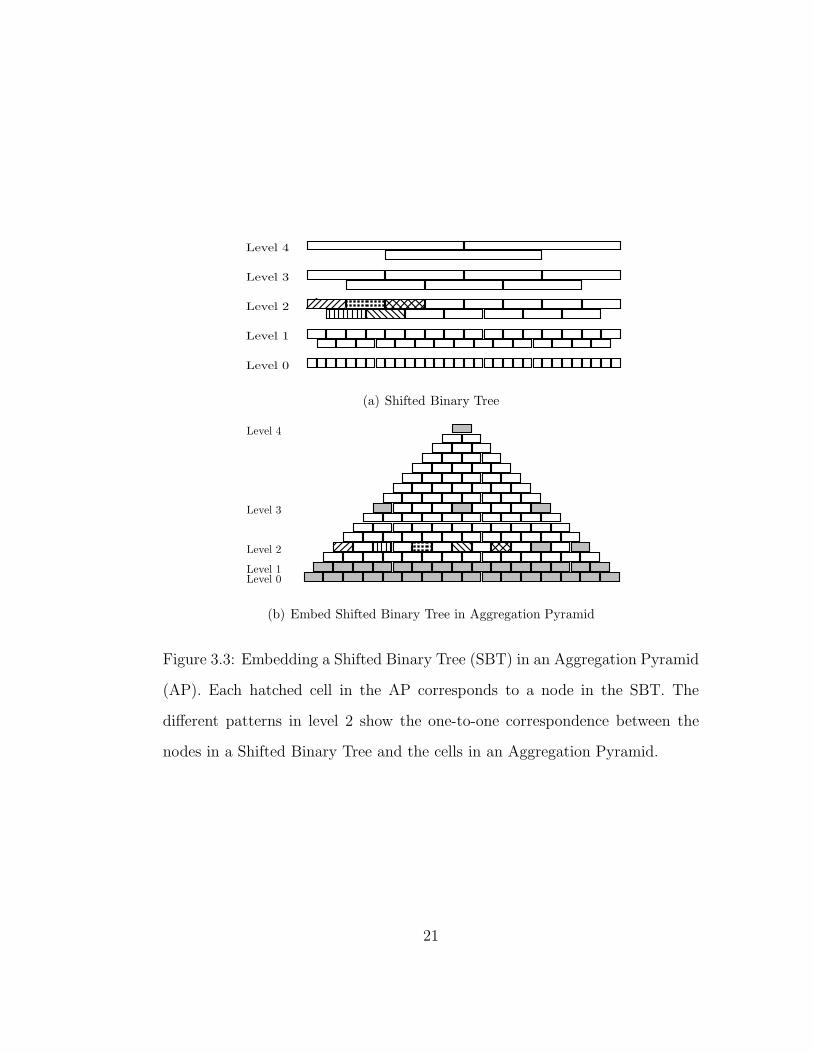
Figure 3.12: The effect of β in the exponential distribution

44

As λ, i.e. (µ/σ)2, increases, Pa increases. More detailed searches are

performed so the CPU time increases. To mitigate this, the Shifted Ag-

gregation Tree must become denser in order to bring down the alarm

probability. When λ becomes very large, the alarm probability is close to

1 anyway, so the Shifted Aggregation Tree becomes sparse again to reduce

the updating time, but is essentially useless.

For an exponential distribution with scale parameter β, both µ and λ are

β, so the ratio is the constant 1. This means that changing β should have

no effect on the alarm probability. Figure 3.12 shows the effect of different

β. The experiments show that varying β has no noticeable effect.� The smaller the burst probability p, the larger the threshold, the smaller

Pa.

This essentially moves the threshold line of size w to the right in Figure

3.10. So Pa decreases.

Figure 3.13 and 3.14 show the effect of different thresholds for the Pois-

son distribution and the exponential distribution respectively. The burst

probabilities range from 10−2 to 10−10. As the burst probabilities go down,

both the alarm probabilities and the densities decrease, because there are

fewer bursts to worry about, so speed depends on reducing the update

time.� As the bounding ratio T decreases, so does Pa.

In a Shifted Aggregation Tree, T could be very close to 1, e.g. W = w+1,

whereas T in a Shifted Binary Tree is designed to be about 4. Figure 3.15.a

shows the bounding ratios at different levels of a Shifted Aggregation Tree

45

CPU Time vs. Threshold - Poisson

0

10000

20000

30000

40000

2 3 4 5 6 7 8 9 10

Burst Probability p=10-k

CP

U T

ime (m

s)

SAT

SBT

(a) CPU time

Alarm Probability vs. Threshold - Poisson

0

0.2

0.4

0.6

0.8

1

1.2

2 3 4 5 6 7 8 9 10

Burst Probability p=10-k

Ala

rm p

robabili

ty

SAT

SBT

(b) Alarm Probability

Density vs. Threshold - Poisson

0

0.05

0.1

0.15

0.2

2 3 4 5 6 7 8 9 10

Burst Probability p=10-k

Density

SAT

SBT

(c) Density

Figure 3.13: The effect of burst probability in the Poisson distribution

46

CPU Time vs. Threshold - Exponential

0

5000

10000

15000

20000

2 3 4 5 6 7 8 9 10

Burst Probability p=10-k

CP

U T

ime (m

s)

SAT

SBT

(a) CPU time

Alarm Probability vs. Threshold - Exponential

0

0.2

0.4

0.6

0.8

1

1.2

2 3 4 5 6 7 8 9 10

Burst Probability p=10-k

Ala

rm p

robabili

ty

SAT

SBT

(b) Alarm Probability

Density vs. Threshold - Exponential

0

0.01

0.02

0.03

0.04

0.05

2 3 4 5 6 7 8 9 10

Burst Probability p=10-k

Density

SAT

SBT

(c) Density

Figure 3.14: The effect of burst probability in the exponential distribution

47

Bounding Ratio vs. Level in the SAT

0

2

4

6

8

10

12

14

1 2 3 4 5 6 7 8 9 10 11 12 13 14 15 16 17

Level in SAT

Boundin

g R

atio

SBT

10^-3

10^-5

10^-7

10^-9

(a) The bounding ratio for different levels in a Shifted

Binary Tree and Shifted Aggregation Trees for different

burst probabilities

Alarm Probability vs. Level

0

0.2

0.4

0.6

0.8

1

1.2

1 3 5 7 9 11 13 15 17 19 21

Level in the SAT

Ala

rm p

robabili

ty

SAT

SBT

(b) Alarm probability as a function of window size in the

Shifted Binary Tree vs. the Shifted Aggregation Tree

Figure 3.15: How the bounding ratio in a Shifted Aggregation Tree adjusts as a

function of window size and the burst probability in order to reduce the alarm

probability.

48

and a Shifted Binary Tree under different burst probabilities. Notice how

the bounding ratio changes in a Shifted Aggregation Tree: it is high at

the lower levels where the window size w is small, while low at the higher

levels where the window size w is large, in order to bring down the alarm

probability. As the burst probability becomes smaller, there are fewer

bursts. Thus, the bounding ratio becomes a little larger, and the Shifted

Aggregation Tree becomes sparser.� As the size w increases, so does Pa.

Figure 3.15.b shows the alarm probabilities at different levels in a Shifted

Binary Tree and a Shifted Aggregation Tree. The Shifted Binary Tree

always has a high alarm probability at the high levels, while in a Shifted

Aggregation Tree, by using a small bounding ratio T , the alarm probability

remains low. Thus the Shifted Aggregation Tree has more filtering power

than the Shifted Binary Tree.

In summary, because the Shifted Aggregation Tree can adjust its structure

to reduce the alarm probability, it achieves far better running time than the

Shifted Binary Tree.

Search parameters in the state-space algorithm

We want to study how different search parameters affect the desired Shifted

Aggregation Tree structures in the state-space algorithm. We tested on different

data settings with different numbers of final states and different number of states

with the same maximum window size, to see when there are diminishing returns

from broadening the search.

49

10

100

750

SB

T

Exp0.05

Poisson10

5000

10000

15000

20000

CPU Time

(ms)

Search Parameter

Dataset

CPU Time vs. Search Parameter

Exp0.05

Exp5

Exp500

Poisson0.1

Poisson1

Poisson10

Figure 3.16: CPU time for Shifted Aggregation Trees found using different

search parameters

The number of states with the same maximum window size, and the number

of final states are set to be 10, 50, 100, 500, 750, 1000 respectively. Other

parameters are chosen randomly to cover a broad parameter range. Table 3.3

summarizes the parameter settings. Three pieces of training data are picked for

the Poisson distribution and the exponential distribution respectively. Figure

3.16 shows the CPU running times for the Shifted Aggregation Trees found

using these parameters. It also shows the CPU running time for the Shifted

Binary Tree as a reference.

The experiments show that even with small values of these parameters, the

Shifted Aggregation Trees discovered are close to those discovered with much

larger values of the parameters. The best-first search strategy works well in this

situation. In practice, we believe that setting both parameters to be 500 works

most effectively.

50

Table 3.3: Statistics for testing data sets for search parameters

Mean StdDev Max Number of Burst

Size Sizes Probability

Poisson0.1 0.1 0.316 250 250 10−3

Poisson1 1 1 750 25 10−5

Poisson10 10 3.16 500 100 10−6

Exponential0.05 0.05 0.05 500 500 10−5

Exponential5 5 5 750 75 10−7

Exponential50 500 500 1000 50 10−8

51

Chapter 4

Greedy Dynamic Burst

Detection

The previous chapter shows a framework to train a Shifted Aggregation Tree

given a sample input time series and window thresholds. However in real world

situations, the incoming data often changes constantly.

In a situation where the input time series keep changing, the performance

would be poor if the training data used to find the Shifted Aggregation Tree

differed significantly from the data to be detected. For example, if the training

data has fewer bursts, as with a trained Shifted Aggregation Tree that is sparse,

while the test data has far more bursts, it would require a denser structure. If

the training data has the same mean and standard deviation as those of the

test data, we call it an unbiased data (thus an “ideal” training data), otherwise

we call it a biased data. Our experiment (Figure 4.3) shows that given fixed

thresholds, the detection time training with a biased data can be 10 percent to

2.5 times more than that training with an unbiased data. In this case, it would

be preferable if we could dynamically adjust the structure in order to achieve

52

better performance.

In this chapter, we present a greedy dynamic detection algorithm which

dynamically evolves the Shifted Aggregation Tree to adapt to the incoming

data. This algorithm starts with a Shifted Aggregation Tree trained with a

sample data set from the incoming data, then changes the structure dynamically

based on the alarms to trigger a detailed search. The dynamic structure either

filters out more detailed searches or reduces the number of updates, and thus

has better detection time. The experiments show that the dynamic algorithm

overcomes the discrepancy resulting from a biased training set and achieves even

better performance than the static algorithm training with an unbiased sample

data in most cases.

This chapter is organized as follows: Section 4.1 describes the structural

dependency between different levels in a Shifted Aggregation Tree and defines

a more flexible dependency structure which can be easily changed dynamically.

Section 4.2 presents the greedy dynamic detection algorithm. The experimental

results are shown in Section 4.3 comparing the greedy algorithm with the static

algorithm over different settings and different types of data. A worst-case anal-

ysis comparing the greedy algorithm with the clairvoyant algorithm is presented

in Section 4.4.

4.1 Structural Dependency

In the state-space search algorithm, the candidate Shifted Aggregation Tree

keeps growing by adding one level onto the top of the existing candidate tree.

For example, a level of window size 256 can be added onto the top of a Shifted

Binary Tree with maximum window size of 192 by adding an extra window of

53

size 64. There is a structural dependency between the levels. For example, a

window of size 256 won’t be computed without its children subwindows of size

192 and size 64, therefore we cannot remove the level of size 192 if the level of

size 256 is still in the tree. Because each level depends on one level below, we

don’t have complete freedom in removing levels.

However, it is easy to see that one window can be composed of different sets

of subwindows, for example, a window of size 256 can be composed of one of

size 192 and one of size 64, or two of size 128. Therefore, we can construct the

Shifted Aggregation Tree in such a way that only a small set of backbone levels

are used to compose other levels. An example of the backbone levels are levels

of sizes 16, 32, 64, 128, etc. By aggregating these backbone levels, we can get

other window sizes such as 48, 96, 192, etc. These window sizes in turn can act

as the secondary backbone levels to compose more window sizes, for example a

window of size 112 (aggregating size 16 and 96).

Figure 4.1 shows the algorithm to reformat a Shifted Aggregation Tree gen-

erated by the state-space algorithm in order to reduce the structural depen-

dency. “Reformatting” entails changing the dependency relationships among

levels. “Occurrence” in this context means how many times a level appears as

a child of higher levels. For example, in the original structure shown in Table

4.1, the occurrence of size 8 is 2, the occurrence of size 16 is 6, the occurrence

of size 48 is 1, etc.

The basic idea is first to pick a level L with the most occurrences in the tree

but having the minimum window size. That level L is reformated to depend

on the 0th level. L is then called the base level. In general, a level which can

be computed from the set of reformated levels only and having the minimum

number of unique children is reformated to depend on these children. This

54

count the occurrences of the child levels of every level

L = {all levels but level 0}; // levels to be reformated

R = {}; // reformated levels

while L not empty

let k be the level in L with the most occurrences

but having the minimum window size

reformat k to depend on level 0 only

move k from L to R

D = {l: l ∈ L, level l can be composed of by levels in R only}

while D not empty

m = the level in D having minimum number of unique children

reformat m to be the aggregate of these children

move m from L to R, remove m from D

update D

end while

end while

Figure 4.1: Algorithm to reformat the parent-child structures in order to reduce

the structural dependency in a Shifted Aggregation Tree

55

process is repeated until all the levels are reformated.

Table 4.1 shows an example of how the algorithm reformats a Shifted Ag-

gregation Tree. The algorithm first picks the level of size 16 as the base level.

Because size 16 depends on size 1 only, size 8 is removable. Next size 32 which

depends on size 16 only is picked as the second level, and similarly for size 64

and size 128 in turn. Finally, other levels are reformated to depend on these

reformated levels only.

In this way, we organize all the window sizes in dependency hierarchies. The

bottom hierarchy contains the backbone levels; the second hierarchy contains

the levels that are dependent only on the bottom hierarchy; the levels in a higher

hierarchy depend only on the levels in the same or lower hierarchies; and so on,

until the top hierarchy which has no other levels depending on them. This way

there are fewer dependencies between different levels, giving us the freedom

to add or remove levels on the fly. We can change the structure from a very

sparse one that contains only the initial backbone levels to a very dense one that

contains many derivative levels, or any structure in between. In other words,

we can create multiple different structures on the fly with different maintenance

costs and different pruning power to adapt to different incoming data.

When trying to add a level in between two levels, say of size 128 and size

256, we want to add the level in such a way that it has good pruning power (to

potentially save more detailed search time) and it has low updating cost and

less dependency (to save more updating time). We prefer a level which is evenly

spread out in between these two levels and belongs to as low of a hierarchy as

possible. For example, we prefer to add a level of size 192 between size 128 and

size 256, instead of 144, because given the same cost to update, a window of

size 192 can avoid more detail searches if there is no alarm raised. We prefer

56

Table 4.1: An example of reformating a Shifted Aggregation Tree to reduce

structural dependency

Step 0: original structure Step 1: size 16 picked as the base level

size children

1 1

8 depending on size 1 only

16 8+8

32 16+16

48 16+32

64 16+48

80 16+64

96 16+80

128 32+96

size children

1 1

8 depending on size 1 only

16 depending on size 1 only

32 16+16

48 16+32

64 16+48

80 16+64

96 16+80

128 32+96

Step 2: size 32, 64 and 128 reformated Step 3: other levels reformated

size children

1 1

8 depending on size 1 only

16 depending on size 1 only

32 16+16

48 16+32

64 32+32

80 16+64

96 16+80

128 64+64

size children

1 1

8 depending on size 1 only

16 depending on size 1 only

32 16+16

48 16+32

64 32+32

80 16+64

96 32+64

128 64+64

57

not to add a level of size 193, because its pruning power is similar to 192, but

depends on more levels, thus requiring more updating cost and restricting the

removal of other levels. We denote the candidate level to be added between

two levels of size hi and hi+1 as cand(hi, hi+1). cand(hi, hi+1) is chosen from

all the possible levels between hi and hi+1, based on the above criteria. After

cand(hi, hi+1) is chosen, the same process is used to choose the new candidate

level between hi and cand(hi, hi+1), and the one between cand(hi, hi+1) and

hi+1. This is repeated until no more levels can be added between two adjacent

levels. In order to efficiently retrieve the candidate levels, in the initialization

phase, a map is constructed; this map maps two adjacent levels to the candidate

level to be added in between.

4.2 Greedy Dynamic Detection Algorithm

Before going into the algorithm details, we first explain the cluster and delay

phenomenon when an alarm happens. This phenomenon is used as a heuristic

in the dynamic algorithm.

Alarms are likely to happen in clusters, across multiple window sizes and

multiple neighboring windows. When a large number of events happen in a short

period of time, the number of events in any window containing this period of

time is likely to be large too, due to the monotonicity property. For example, a

window of size 5 contains 30 events and raises an alarm because it exceeds the

threshold of 10 events for size 5. A window of size 10 containing this window of

size 5 would likely contain a large number of events and thus also raise an alarm.

In this case, multiple neighboring windows of different sizes may exceed their

minimum thresholds and raise alarms. Furthermore, when a burst happens in a

58

Table 4.2: Weights used for different operations in the dynamic algorithm

updating filtering detailed search changing structure

4.6 1 2.1 10

small window, a larger window starting with this small subwindow likely raises

an alarm some time later when the larger window ends. In the above example,

the alarm at size 10 will be raised 5 time points later than the alarm at size

5. In other words, there is some delay for an alarm at a larger window size

following an alarm at a smaller window size.

This phenomenon suggests when an alarm happens at level k, we may ex-

pect more alarms at levels higher than k in the near future. Accordingly, the

structure should be changed so as to anticipate this.

The basic idea behind the dynamic detection algorithm is to change the

Shifted Aggregation Tree if a change helps to reduce the overall cost. In order

to compute the cost, we use the theoretical model as described in the previous

chapter. Besides the costs for updating, checking/filtering and detail searches,

there will be a cost for changing the structure. We use a similar test run

method as described in the theoretical model section to quantify this cost. We

run the operation a million times to change one level (i.e. add/remove a level

or widen/narrow a shift as defined below) in the Shifted Aggregation Tree. The

average CPU time is used as the unit cost for changing a level. Table 4.2 shows

the cost for changing the structure compared to other operation costs. Note

that the cost to change one level is not that significant compared to other costs.

This allows us to change the structure relatively frequently.

Intuitively, when considering one level alone, if by adding a level, the total

saved detailed search cost is more than the total updating/filtering cost plus

59

the cost to change the structure, we should add this level. Similarly, if the

updating/filtering cost for a level is greater than the detailed search cost it saves

and the changing cost, we should remove this level. However, when considering

multiple levels together, this removed level may have been helpful for supporting

another higher level which would in turn have saved more detail searches. For

example, a level of size 64 may support a level of 192 which aggregates size 64

and size 128.

We adopt a greedy strategy when trying to make the structure denser, i.e.

whenever the saved detail search cost is greater than the updating/filtering

cost, make the structure denser. On the other hand, because of the cluster and

delay phenomenon, we use a delayed greedy strategy when trying to make the

structure sparser: if an alarm is raised at level k at time t, we won’t remove

any level lower than k + δk until time t + δt, where δk ≥ 0, δt ≥ 0. This

is to anticipate any potential secondary alarm after an alarm occurs and to

avoid unnecessary changes to the structure. We call this region determined by

δk and δt an alarm region. The alarm region extends further if a new alarm

occurs in the alarm region. We will study the effect of different δk and δt in the

experiment section.

To make a structure denser, we can add a level or make a shift smaller;

conversely, we can remove a level or make a shift larger to make a structure

sparser. Recall that a shift is defined as the number of time points separating

two neighboring nodes at the same level. The closer two neighboring nodes are,

the denser the structure is. Due to the Shifted Aggregation Tree property, the

shift at level k+1 has to be an integral multiple of the shift at level k. So, when

changing a shift Sk, we make the new shift either 2Sk (i.e. double the current

shift) or Sk

2(i.e. half the current shift). This normally satisfies the integral

60

multiple property (it always does for halving and often does for doubling in our

construction method).

To be more specific, we need to decide the following:� Which structure to start with:

Given the inputs, we first train a Shifted Aggregation Tree using any sam-

ple data set. Then we reformat the Shifted Aggregation Tree to reduce the

structure dependency as described in the structural dependency section.

The dynamic algorithm starts with the reformatted structure.� How to change the structure:

We define four possible actions to change level k in the existing structure:

– Add a level between level k and level k − 1

– Remove level k

– Widen the shift at level k, denoted by Sk, to be 2Sk

– Narrow the shift at level k, denoted by Sk, to be Sk

2

Notice that all these actions have to conform to the dependency rules. Also

the structure after the change has to be another valid Shifted Aggregation

Tree, i.e. they have to satisfy the properties of a Shifted Aggregation Tree

as described in the framework chapter.

Theoretically, we can narrow or widen the shift of a level as long as

the structure after the change is still a valid Shifted Aggregation Tree.

However in the actual implementation, a memory buffer is allocated to

store the aggregate for one level. The narrow operation requires a mem-

ory reallocation and re-creation of the parent-children structure which

61

are expensive operations. One way to avoid the memory reallocation

is to allocate a larger buffer than needed when first creating this level.

We still need to restrict the maximum allowed shift step ms such that

1ms

≤ shift at any time

initial shift≤ ms, i.e. the shift won’t be ms times more than the

initial shift or 1/ms times less than the initial shift. It actually limits how

many times we can consecutively widen or narrow a shift from the initial

shift, thus how far a structure can change away from the initial structure.

For example, the initial shift for a level is 32 time points, if ms is set to

be 1, the shift can be 16, 32 and 64; if ms is set to be 2, the shift can be

8, 16, 32, 64 and 128; and so on. We will show the effect of the maximum

allowed shift step in the experiment section. A too large ms actually may

lead to poor performance depending on how far the training data deviates

from the test data.� When to change the structure:

– When an alarm is raised at some level k + 1 and a detailed search is

triggered, we check if adding cand(hk, hk+1) will help to reduce the

cost for detailed search. If the cost saved on the detailed search is

greater than the updating/filtering cost, we add this candidate level

between level k and k + 1.

– If the candidate level cannot be added because some of its children

are not in the tree, then add those children into the tree.

– If the candidate level cannot be added because its shift makes the

resulting structure invalid, we try to narrow the shifts of levels below

k +1 if narrowing the shifts is helpful to fit the candidate in. For ex-

ample, based on the Shifted Aggregation Tree properties, we cannot

62

add a level of size 20 with shift 8 between a level of size 24 with shift

8 and a level of size 16 with shift 8, because the overlapping size of

the level of size 20 has to be greater than or equal to size 16. In this

case, we first narrow the shifts at these three levels (16, 20, 24) to be

4. This allows more candidate levels to be added in.

– If the aggregate at level k+1 does not exceed the minimum threshold

for level k, i.e. keeping the level k does not help to reduce the detailed

search time, we remove level k if it is not in an alarm region.

– If level k cannot be removed due to the dependency and it is not in

an alarm region, we try to widen and double the shift at level k if

possible.

Figure 4.2 shows the full detection algorithm.

4.3 Empirical Results

We have tested the greedy dynamic detection algorithm on different types of

data distributions and different parameter settings. The experiments show that

the greedy dynamic detection algorithm overcomes the discrepancy resulting

from a biased training data and achieves better performance in most cases than

the static algorithm even training with unbiased sample data. But it may not

work as well as the static algorithm in some cases, for example when the bursts

are very rare or very frequent.

First we compare the performance of the dynamic algorithm and the static

algorithm under different parameter settings. Then we also study the effect of

different parameters in the dynamic algorithm: the maximum allowed shift step

63

for every time point t starting from 1

al = 0; as = 0; alarm region = null;

for the window ending at the current time t at every level i

update node(i, t) by aggregating its children

if node(i, t) raises an alarm then

if legal to add cand(hi−1, hi)

compute the aggregate at cand(hi−1, hi)

if the updating/filtering cost < the saved

detailed search cost by adding cand(hi−1, hi) then

add cand(hi−1, hi) between level i − 1 and i

if cand(hi−1, hi) raises an alarm then

search the DSR of cand(hi−1, hi) for real bursts

else if cannot add because the children are not in the tree

add those children into the tree

else al = i; as = the shift to make cand(hi−1, hi) fit in

if there is still an alarm in the DSR of node(i, t)

search DSR(i, t) for real bursts

update the alarm region

else if node(i, t) < the minimum threshold in DSR(i− 1, t)

and node(i − 1, t) not in the alarm region then

if legal to remove level i − 1 then remove it

else legally double the shift at level i − 1

for i = 1 to al

if shifti > as and legal to narrow shifti, then narrow shifti

Figure 4.2: Greedy dynamic detection algorithm

64

and the size of the alarm region.

In the following experiments, we use the synthetic data with Poisson distri-

bution and exponential distribution as described in the previous chapter. The

experiments on the real world data can be found in the next chapter.

4.3.1 Performance Test

We want to compare the performance of the dynamic algorithm with that of the

static algorithm under different parameter settings: different training data in the

static algorithm, different distribution parameters, different burst probabilities

and different sets of window sizes. Further, we study how the dynamic algorithm

performs under different changing rates and different changing magnitudes in

the data. In the dynamic algorithm, the maximum allowed shift step is set to

be 1 and the size of the alarm region is set to be δk = 1, δt is set to be the size

difference between level k and level k + 1 (as explained later).

Performance comparison using different training sets

Given the fixed thresholds and the test data, we are interested in how differ-

ent training data affect the performance of the static algorithm and how the

dynamic algorithm performs compared to the static algorithm.

A set of Poisson data of 10,000 points are synthesized with different λ: 0.8,

0.9, 1.0, 1.1, 1.2. They are used as the training data in the static algorithm.

A synthesized data of 5 million points with λ = 1 is used as the test data.

The thresholds are computed based on λ = 1 and burst probability 10−6. A

burst probability of p means that for every window size, the probability at any

timepoint that a burst occurs is p. Put another way, we set the threshold for

65

any window size w so that, given the distribution assumptions, the burst occurs

with probability p. The maximum window size is set to be 250; the task is to

detect bursts at every window size.

We use the synthesized data and the same thresholds to train a Shifted

Aggregation Tree in each case. Then the static algorithm is tested with the

trained structure to detect the same test data. Thus except for the training

data having λ = 1, all other training data have different statistics from the test

data, i.e. they are all biased training data.

Similarly, we synthesized a set of training data of exponential distribution

with different β: 0.8, 0.9, 1.0, 1.1, 1.2. Other parameters are set up in the same

way as those for the Poisson data.

Figure 4.3 shows that for the static algorithm, using biased training data

could require 10 to 250 percent more detection time compared to using a un-

biased training data. The dynamic algorithm can reduce the detection time by

up to two-thirds, when the training data differs from the test data significantly.

It even performs about 20 percent better than the static algorithm using the

unbiased training data.

Since biased data always gives worse performance than an unbiased data,

in the next experiments, we show only the comparison between the dynamic

algorithm and the static algorithm using unbiased sample data unless otherwise

stated.

Performance comparison using different distribution parameters

We want to study how the dynamic algorithm performs compared to the static

algorithm using unbiased sample data under different distribution parameters.

As shown in the previous chapter, the parameter in the exponential distribution

66

CPU time for different training sets vs. dynamic

algorithm - Poisson

0

1000

2000

3000

4000

5000

6000

7000

0.8 0.9 1 1.1 1.2

Training Sets with different l

CP

U T

imes (m

s)

static

dynamic

(a) Poisson distribution

CPU time for different training set vs. dynamic

algorithm - Exponential

0

2000

4000

6000

8000

0.8 0.9 1 1.1 1.2

Training sets with different b

CP

U tim

e (m

s) Static

Dynamic

(b) Exponential distribution

Figure 4.3: Performance comparison between the dynamic algorithm and the

static algorithm using different training sets

67

has little effect on the alarm probability. So we show only the results for the

Poisson data.

We synthesized a set of training data with different λ values ranging from

10−3 to 103. Different thresholds and test data are generated based on the

corresponding λ. The burst probability is set to 10−6. The maximum window

size is set to be 250; the task is to detect bursts at every window size.

Notice that the differences between this test and the previous one are the

different thresholds and different test data used. In this test, for λ = 10−1, the

thresholds are generated using mean 10−1 and standard deviation√

10−1; while

in the previous test, the thresholds are generated using mean 1 and standard

deviation 1. Similarly, the test data are generated using λ = 10−1, instead of

using λ = 1. Thus, in this test, the training data are all unbiased.

Figure 4.4 shows the results. When λ is smaller than 100, the dynamic

algorithm performs about 10 percent better than the static algorithm. When

λ is equal to and greater than 100, the dynamic algorithm performs slightly

worse than the static algorithm. The reason is that when λ is large, the alarm

probability is always large, thus the desired structure is sparse to save some

updating time. (Please refer to the previous chapter for the explanation.) The

dynamic algorithm checks to determine if adding a level is helpful each time an

alarm is raised, but most checks are fruitless and a level is seldom added. The

dynamic algorithm saves little by adding a level, instead, it has to spend extra

time on checking to see if adding a level is helpful.

Performance comparison under different burst probabilities

This test compares the dynamic algorithm against the static algorithm using

unbiased data under different burst probabilities.

68

CPU time for dynamic and static algorithm vs. l -

Poisson

0

5000

10000

15000

20000

-3 -2 -1 0 1 2 3

lC

PU

Tim

ie (m

s)

dynamic

static

Figure 4.4: Performance comparison between the dynamic algorithm and the

static algorithm using unbiased data under different distribution parameters

λ is set to be 1 in the Poisson distribution and β is set to be 10 in the

exponential distribution. The burst probabilities range from 10−2 to 10−10.

The maximum window size is set to be 250; the task is to detect bursts at every

window size.

The results in Figure 4.5 show that under different burst probabilities using

unbiased training data, the dynamic algorithm always performs 10 to 20 percent

better than the static algorithm.

Performance comparison under different sets of window sizes of in-

terest

In this experiment, different sets of window sizes of interest are used to see

how the dynamic algorithm performs compared with the static algorithm when

training with unbiased data.

Instead of detecting bursts at every window size, this test detects bursts

only for a set of n window sizes exponentially evenly-spaced up to the maximum

window size of interest, i.e. {N 1

n , N2

n , N3

n , . . . , N}, where N is the maximum

69

CPU time for dynamic and static algorithm vs.

threshold - Poisson

0

2000

4000

6000

8000

-2 -3 -4 -5 -6 -7 -8 -9 -10

Burst Probability p=10-k

CP

U T

ime (m

s)

Static

Dynamic

(a) Poisson distribution

CPU time for dynamic and static algorithm vs.

threshold - Exponential

0

5000

10000

15000

20000

-2 -3 -4 -5 -6 -7 -8 -9 -10

Burst Probability p=10-k

CP

U T

ime (

ms) Static

Dynamic

(b) Exponential distribution

Figure 4.5: Performance comparison between the dynamic algorithm and the

static algorithm training with unbiased data under different burst probabilities

70

window size of interest. In this test, N is set to be 1000 and n is set to be 10,

25, 50, 75, 100 respectively. λ is set to be 0.1 and the burst probability is set to

be 10−4 for the Poisson distribution; β is set to be 10 and the burst probability

is set to be 10−7 for the exponential distribution.

Figure 4.6 shows the results. When n is small, there are fewer window sizes

of interest, and the structure is sparse. In this case, there is little saving for the

dynamic algorithm. Instead, it has to spend more time checking whether or not

it is beneficial to add a level. When n is large, the dynamic algorithm shows its

strength by filtering out unnecessary detailed searches and thus achieves better

performance than the static algorithm.

Performance comparison under different changing rates

The purpose of this experiment is to study how the dynamic algorithm performs

on data with different changing rates. We synthesize five pieces of test data with

different changing rates. Each piece of data contains several segments of data,

each segment has length L. The λ parameter for the ith segment is 0.1 when i

is odd or 1 when i is even, i.e. λ changes every L time points. A larger L means

a slower change in the data, and vice versa. L is set to be 500, 1000, 2000,

4000, 8000 respectively for each piece of data. The total length of each piece of

test data is set to be same, one million points. A segment of 32000 points in

each piece is used as the training data. The maximum window size of interest

is set to be 250; the task is to detect bursts at every window size. The burst

probability is set to be 10−5.

Figure 4.7 shows the results for both the static algorithm and the dynamic

algorithm, together with the difference of the CPU times. For the static al-

gorithm, the experiments show that as L increases, i.e. the changing rate de-

71

CPU time for different sets of window sizes -

Poisson

0

1000

2000

3000

4000

5000

10 25 50 75 100

Number of window sizes

CP

U tim

e (m

s)

Static

Dynamic

(a) Poisson distribution

CPU time for different sets of window sizes -

Exponential

0

1000

2000

3000

4000

5000

10 25 50 75 100

Number of window sizes

CP

U tim

e (m

s)

Static

Dynamic

(b) Exponential distribution

Figure 4.6: Performance comparison between the dynamic algorithm and the

static algorithm using unbiased data under different sets of window sizes

72

CPU times for different changing rates

0

200

400

600

800

500 1000 2000 4000 8000

Segment length C

PU

tim

e (m

s)

static

dynamic

difference

Figure 4.7: The effect of different changing rates. The longer each segment

length, the slower the changing rate.

creases, the CPU time increases, although the number of real bursts actually

decreases from L = 1000 to L = 8000. This occurs because when L is large,

there are more aggregates that have large values, for example, in a segment of

10 consecutive 1s followed by 10 consecutive 0.1s, there are 5 aggregates of size

6 whose value is greater than 5; while in a segment of length 20 with 1 and 0.1

alternating, there is no aggregate of size 6 whose value is greater than 5. Thus,

there are likely more aggregates exceeding their minimum thresholds and more

detailed searches triggered.

On the other hand, there is no such effect using the dynamic algorithm, be-

cause whatever value L has, the dynamic algorithm can add the levels necessary

to filter out unnecessary detailed searches. Therefore, as L increases, the time

the dynamic algorithm saves compared to the static algorithm increases too.

Performance comparison under different changing magnitudes

In this experiment, we want to study how the dynamic algorithm performs

on data with different changing magnitudes. We synthesize five pieces of test

73

CPU times for different changing magnitudes

0

500

1000

1500

0.001 0.01 0.1 1 10

l for the even segmentsC

PU

tim

e (m

s)

static

dynamic

difference

Figure 4.8: The effect of different changing magnitudes. The more λ deviates

from 0.01, the larger the changing magnitude.

data with different changing magnitudes. Each piece of data contains several

segments of data, each having a fixed length of 2000. λ for the ith segment is

set to be 0.1 when i is odd, or 0.001, 0.01, 0.1, 1, 10 respectively for each piece

of data when i is even, to simulate different changing magnitudes. That is, λ

is 0.001 for i at 2, 4, 6, etc. in the first data, and λ is 0.01 for i at 2, 4, 6,

etc. in the second data, and so on. In other words, the first data set consists

of alternating segments characterized by parameters 0.1 and 0.001, the second

data set consists of alternating segments characterized by parameters 0.1 and

0.01, and so on. So, 0.1 means no change at all between the odd segments and

the even segments, while 0.001 and 10 have the largest changing magnitudes.

The total length of each piece of test data is set to be the same, one million

points. A segment length of 32000 points in each piece is used as the training

data. The maximum window size of interest is set to be 250; the task is to

detect bursts at every window size. The burst probability is set to be 10−5.

Figure 4.8 shows the results for both the static algorithm and the dynamic

algorithm, together with the difference of the CPU times. Although the number

74

of real bursts are different in each test data, the experiments show that as the

changing magnitude increases, the time the dynamic algorithm saves compared

to the static algorithm increases too. Because each test data is composed of two

sets of data with different parameter settings, each set of data is best served by a

different Shifted Aggregation Tree. When there is a large difference between the

parameters, i.e. the magnitude change is large, there is also a large difference

between the desired structures. While the static algorithm has to use a structure

compromising between these two desired structures, the dynamic algorithm can

change from one structure to another on the fly, and thus save more running

time.

In summary, the dynamic algorithm overcomes the discrepancy resulting

from a biased training data. In most cases, it performs better than the static

algorithm training even with unbiased data. However, when the bursts are either

very rare or very frequent, it may perform worse than the static algorithm. The

greater the change in magnitude, the slower the changing rate, the more the

dynamic algorithm saves compared with the static algorithm.

4.3.2 The effect of the parameters in the dynamic algo-

rithm

In this section, we study the effect of the parameters in the dynamic algorithm.

We picked 6 test settings to simulate different scenarios as shown in Table 4.3.

The effect of the maximum allowed shift step

As stated in the algorithm section, the dynamic algorithm allows changing a

structure by widening or narrowing the shifts. A shift is the number of time

75

Table 4.3: Test settings to study the effect of algorithm parameters

Training data Test data Max Number of Burst

parameter parameter size sizes probability

Poisson1 1 0.5 250 250 10−3

Poisson2 1 1 750 25 10−5

Poisson3 5 10 500 100 10−6

Exponential1 0.8 1 250 250 10−6

Exponential2 5 5 750 75 10−7

Exponential3 50 5 1000 50 10−8

points separating two neighboring nodes at the same level. Because of the mem-

ory reallocation and re-creation of the parent-children structure when changing

a shift, we restrict the maximum allowed shift step, i.e. how many times we can

consecutively widen or narrow a shift from the initial shift. For example, one

shift step allowed means that the legal shift can be 16, 32 or 64 if the initial

shift is 32. It can never take other values. This experiment studies how the

maximum allowed shift step affects the performance.

We set the maximum allowed shift step ms to be 0, 1, 2 respectively. The

larger the value, the more a structure is allowed to deviate from the initial

structure. Zero means no widening/narrowing is allowed. Figure 4.9 shows the

results. The CPU running time of the static algorithm is included as a reference.

For some setting where the training data differs greatly from the test data

(for example, Exponential1), the initial structure deviates greatly from the de-

sired structure. For example, the initial shift at a level is 256, but a better

structure would have a shift of 4. A small maximum allowed shift step, say 1,

allows the shift to be 128, 256, or 512, which are still far from the desired shift.

76

CPU time vs. Max Allowed Shift Step

0

2000

4000

6000

8000

10000

12000

14000

Poiss

on1

Poiss

on2

Poiss

on3

Exp1

Exp2

Exp3

Test SettingC

PU

tim

e (

ms

) step=0

step=1

step=2

static

Figure 4.9: The effect of the maximum allowed shift step. The larger the step,

the more a structure is allowed to deviate from the initial structure.

By contrast, a large maximum allowed shift step allows changing the initial

structure greatly, bringing it closer to the optimal structure, and thus achieves

better performance compared to a small value.

However for other settings, the desired structure is close to the initial struc-

ture. When ms is too large, the structure can become very sparse when there

is no burst for a long period of time. In this instance, if a burst starts to hap-

pen, because a shift is only doubled or halved once when a node is updated, the

structure cannot become dense quickly enough to filter out unnecessary detailed

searches and thus has to spend more time in detailed searches. In practice, we

believe generally it works best to set the maximum allowed shift step to be 1,

unless it is known that the training data differs from the test data greatly.

The effect of the size of the alarm region

As described in the algorithm section, when an alarm is raised at level k at

time t, we do not remove any level lower than k + δk until time t + δt, where

δk ≥ 0, δt ≥ 0. The purpose is to be prepared for more coming alarms and thus

77

avoid unnecessary structural changes when an alarm occurs. We want to study

how different δk and δt values affect the performance.

We set δk to be 0, 1, 2 respectively to see the effect of different size ranges,

and set δt to be 0, the size difference between level k and level k + 1, the size

of level k, respectively, to see the effect of different time ranges. Smaller δk

and δt allow the algorithm to remove a level or widen a shift sooner, but may

lead to frequent structural changes. Frequent structural changes may cause the

structure to become sparse and then be unable to become dense quickly enough

to filter out unnecessary detailed searches. By contrast, large δk and δt avoid

frequent structural changes but may be too conservative to make a structure

sparser. The maximum allowed shift step is set to be 1 in this test.

Figure 4.10 shows the results. The CPU running time of the static algorithm

is included as a reference. The results show that medium δk and δt work better

than small or large δk and δt. The small δk and δt have to spend more time

changing the structure and detailed searching, while the large δk and δt cannot

remove the unnecessary levels quickly and have to spend more time updating

the structure.

Given the above experimental results, we recommend the following about

the dynamic algorithm:� If the bursts are very rare or very frequent, e.g. the burst probability is

very low or very high, or the number of window sizes is very few, use the

static algorithm only.� If it is known the training data deviates greatly from the test data, use a

large maximum allowed shift step with the dynamic algorithm. The more

the difference is, the larger this value should be. Otherwise, it is better to

78

CPU time vs. dk in alarm region

0

1000

20003000

4000

5000

6000

7000

8000

Poiss

on1

Poisson

2

Poiss

on3

Exp1

Exp2

Exp3

Test Setting

CP

U tim

e (m

s)

dk=0

dk=1

dk=2

(a) Different δk

CPU time vs. dt in alarm region

0

1000

2000

3000

4000

5000

6000

7000

8000

Poiss

on1

Poiss

on2

Poiss

on3

Exp1

Exp2

Exp3

Test Setting

CP

U tim

e (m

s)

dt=0

dt=h_{k+1}-h_k

dt=h_k

(b) Different δt

Figure 4.10: The effect of the size of the alarm region. The larger δk and δt,

the larger the alarm region.

79

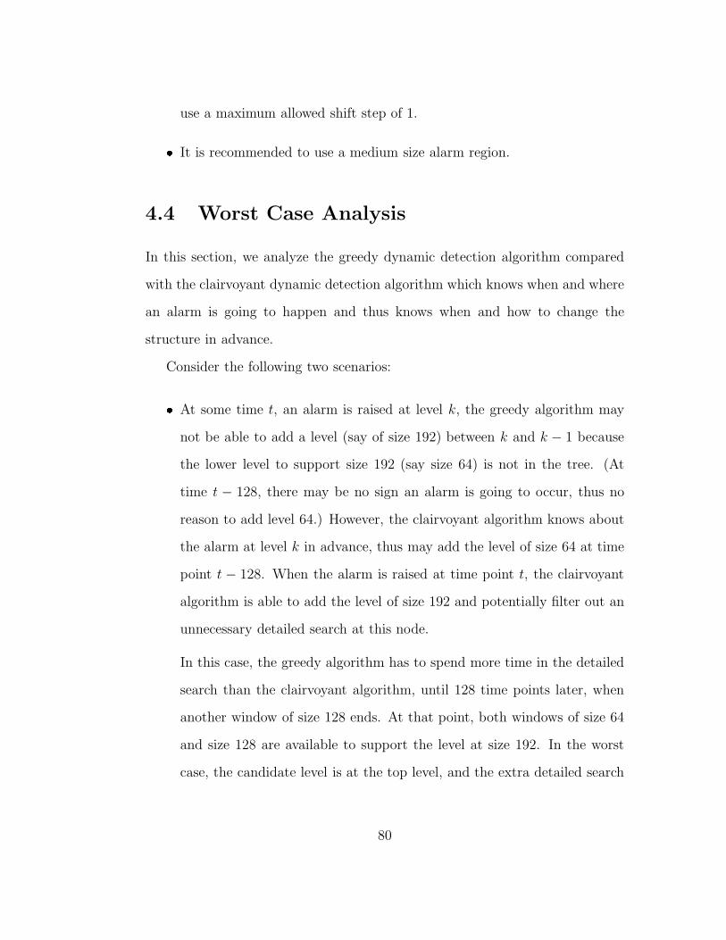
use a maximum allowed shift step of 1.� It is recommended to use a medium size alarm region.

4.4 Worst Case Analysis

In this section, we analyze the greedy dynamic detection algorithm compared

with the clairvoyant dynamic detection algorithm which knows when and where

an alarm is going to happen and thus knows when and how to change the

structure in advance.

Consider the following two scenarios:� At some time t, an alarm is raised at level k, the greedy algorithm may

not be able to add a level (say of size 192) between k and k − 1 because

the lower level to support size 192 (say size 64) is not in the tree. (At

time t − 128, there may be no sign an alarm is going to occur, thus no

reason to add level 64.) However, the clairvoyant algorithm knows about

the alarm at level k in advance, thus may add the level of size 64 at time

point t − 128. When the alarm is raised at time point t, the clairvoyant

algorithm is able to add the level of size 192 and potentially filter out an

unnecessary detailed search at this node.

In this case, the greedy algorithm has to spend more time in the detailed

search than the clairvoyant algorithm, until 128 time points later, when

another window of size 128 ends. At that point, both windows of size 64

and size 128 are available to support the level at size 192. In the worst

case, the candidate level is at the top level, and the extra detailed search

80

has to be performed within the time period from t up to t + W , where W

is the maximum window size of interest.

Notice this could happen at multiple levels at the same time. Therefore

the extra detailed search time is of Θ(mW ), where m is the number of

window sizes of interest.� After an alarm is raised at t, the greedy algorithm will not remove a

level within the alarm region at level k + δk until time t + δt, while the

clairvoyant algorithm may know that there will be no more alarms and

thus will remove this level right away.

In this case, the greedy algorithm has to spend more time in the updat-

ing/filtering phase than the clairvoyant algorithm, until the alarm region

ends. Assuming the underlying data is independent, a window of size W

contains no information about a window of size W following it. Thus δt

should be less than W . The extra updating/filtering cost should be the

cost within a window of size at most W .

Put them together and the worst case scenario would be that the clairvoyant

algorithm does not need any detailed search (i.e. there is no real burst at all),

but the greedy algorithm has to spend more detailed search time when an alarm

starts to occur and more updating/filtering time in the alarm region.

Let tu, ts, tc denote the total updating/filtering time, searching time and

structure-changing time respectively for the greedy algorithm. Similarly, we use

tCu , tCs , tCc to denote the same costs for the clairvoyant algorithm. As explained

above, we need to consider only the costs in a time period of 2W : W for the

period from the start of an alarm to the addition of a candidate level, and

another W for the alarm region.

81

Within the time period 2W , the number of nodes in the tree is of Θ(W ), so

are tu and tCu , since each updating/filtering operation is associated with a node.

Because a change to the structure only happens after a node is updated, tc and

tCc have the complexity of Θ(L), where L is the number of levels in the tree,

L < W . As explained above, the detailed search cost ts for the greedy algorithm

has the complexity Θ(mW ), while tCs is 0 for the clairvoyant algorithm. So in

the worst case, the greedy algorithm has the complexity of Θ(mW ), while the

clairvoyant algorithm has the complexity of Θ(W ). The performance ratio is

up to m, the number of window sizes of interest.

82

Chapter 5

Case Study

In this chapter, we study several real world burst detection applications in

physics, finance and website traffic monitoring. We also show how bursts can

be a primitive for higher-level data mining tasks, such as burst correlation.

Real world applications all confirm the excellent performance of our algorith-

mic framework. The experiments show that the average processing time to

process a new datum is less than 0.1 ms, therefore, the Shifted Aggregation

Tree framework is suitable for real data stream environments.

5.1 Gamma Ray Burst Detection in Astron-

omy

Gamma rays are high-energy electromagnetic radiation produced by radioactive

decay or other nuclear processes. In the cosmos, different processes can generate

gamma ray emissions, such as cosmic ray interactions with interstellar gas,

supernova explosions and interactions of energetic electrons with magnetic fields

83

Figure 5.1: Gamma Ray Burst 971214 (image from Hubble Space Telescope

website [4])

to name a few. Gamma Ray Bursts (GRB) are flashes of gamma rays. They are

the brightest source of cosmic gamma-ray photons in the observable Universe,

hundreds of times brighter than a typical supernova and about a million trillion

times as bright as the Sun. Since the first GRB discovered in the late 1960s,

Gamma Ray Bursts have been important phenomena and useful vehicles for

physicists to study the activity of the Universe. Figure 5.1 shows a picture of a

GRB observed by the Hubble Space Telescope [4].

Gamma Ray Bursts occur roughly once per day from wholly random direc-

tions of the sky. A Gamma Ray Burst can last anywhere from milliseconds to

minutes, even days. For example, the GRB 060218 discovered in February 2006

lasted for 33 minutes, while the GRB 050509 detected in May 2005 only lasted

for a tiny fraction of a second. They can be classified as long-duration bursts

84

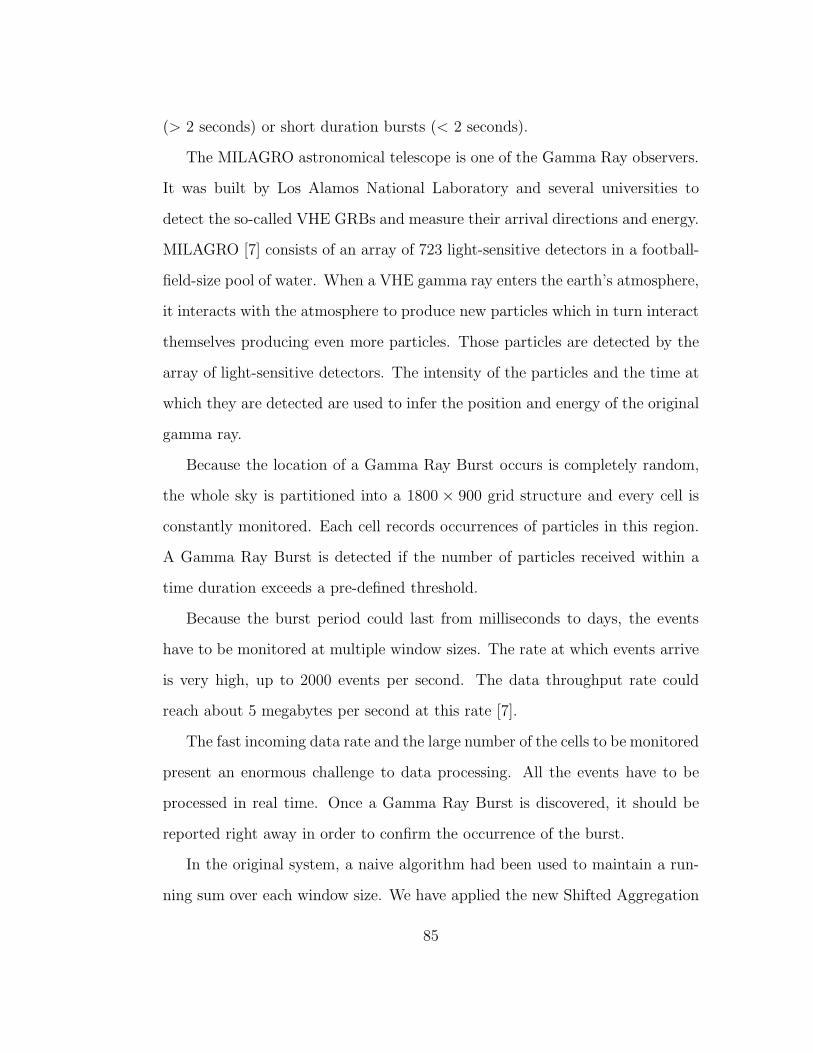
(> 2 seconds) or short duration bursts (< 2 seconds).

The MILAGRO astronomical telescope is one of the Gamma Ray observers.

It was built by Los Alamos National Laboratory and several universities to

detect the so-called VHE GRBs and measure their arrival directions and energy.

MILAGRO [7] consists of an array of 723 light-sensitive detectors in a football-

field-size pool of water. When a VHE gamma ray enters the earth’s atmosphere,

it interacts with the atmosphere to produce new particles which in turn interact

themselves producing even more particles. Those particles are detected by the

array of light-sensitive detectors. The intensity of the particles and the time at

which they are detected are used to infer the position and energy of the original

gamma ray.

Because the location of a Gamma Ray Burst occurs is completely random,

the whole sky is partitioned into a 1800 × 900 grid structure and every cell is

constantly monitored. Each cell records occurrences of particles in this region.

A Gamma Ray Burst is detected if the number of particles received within a

time duration exceeds a pre-defined threshold.

Because the burst period could last from milliseconds to days, the events

have to be monitored at multiple window sizes. The rate at which events arrive

is very high, up to 2000 events per second. The data throughput rate could

reach about 5 megabytes per second at this rate [7].

The fast incoming data rate and the large number of the cells to be monitored

present an enormous challenge to data processing. All the events have to be

processed in real time. Once a Gamma Ray Burst is discovered, it should be

reported right away in order to confirm the occurrence of the burst.

In the original system, a naive algorithm had been used to maintain a run-

ning sum over each window size. We have applied the new Shifted Aggregation

85

Performance comparison - Gamma Ray Burst

Detection

0

200

400

600

800

1000

1200

14 28 42

Number of window sizes of interestC

PU

Tim

e (s) Naive

SBT

SAT

Figure 5.2: Performance comparison between the Shifted Binary Tree and the

Shifted Aggregation Tree on the Gamma Ray Burst data

Tree framework to this situation.

The test data set includes 5 offline raw data files. Each data file contains the

raw observed events including the observed time, signal intensity, position, etc.

There are in total about 2.5 million events. These raw events are first allocated

into one of the 1800 × 900 cells. Then the bursts are detected within each cell.

N window sizes of interest are monitored, N was set to be 14, 28, 42 in this

test. The minimum time resolution to distinguish a burst is 0.01 second. The

minimum window size of interest Nmin is 0.1 second, and the maximum window

size of interest Nmax is 39.8 seconds. The window sizes of interest are exponen-

tially even-spaced between the minimum window size and the maximum win-

dow size, i.e. {exp(Nmin + ln(Nmax−Nmin)n

), exp(Nmin + 2 ln(Nmax−Nmin)n

), exp(Nmin +

3 ln(Nmax−Nmin)n

), . . .}. The thresholds are updated dynamically based on the back-

ground signals in the sky.

We use a small sample of 10K data from the first file to train a Shifted Ag-

gregation Tree. We use the empirical cost model: run 1000 times detection over

this training data and use the actual CPU time as the cost. The trained Shifted

86

Figure 5.3: An example how the price of the S&P 500 Index interacts with the

volume spikes (chart from MarketVolume.com [6])

Aggregation Tree is used for burst detection on the five test data files. Figure

5.2 shows the result. The Shifted Binary Tree outperforms the naive approach

by a factor of 3 to 6, furthurmore, the Shifted Aggregation Tree framework

achieves a 1.5 to 3 times speedup over the Shifted Binary Tree. More speedup

can be achieved if there are more window sizes of interest, which is helpful to

avoid missing any possible burst.

5.2 Volume Spike Detection in Stock Trading

In stock trading, the trading volume is the number of shares or contracts of a

security traded during a given length period. Volume indicates the interest of

87

traders in buying or selling a security. It is the underlying force behind price

movements. For example, a large volume on the buy side suggests a strong

buy interest, thus the price is likely to rise; conversely, a small volume means a

weak interest, suggesting the rise has lost its momentum and the price is likely

to fall. The volume behavior and the price behavior are closely interrelated.

The price pattern can be anticipated by a proper understanding of the volume

pattern. There is a long history of traders using volume as a technical indicator

to analyze stock behavior.

A commonly used volume indicator is Volume Moving Average (VMA). Sim-

ilar to the price moving average, Volume Moving Average is the average of the

trading volume over a given period of time. The VMA can be computed over

several seconds to several months to capture the patterns over different time

scales. Within the smoothed view of the trading volume, a large peak in the

VMA, called Volume Spike, is of particular interest. A volume spike indicates

a burst of trading activity. It is usually triggered by some political or economic

news, earning reports, etc., and may drive the price to change substantially.

Figure 5.3 shows an example of how the price reversals of the Standard & Poor

500 Index interacts with volume spikes.

Due to the time-sensitive nature of the stock market, it is very important

for traders to be able to detect volume spikes as early as possible. In the

modern security industry, there are hundreds of thousands of securities traded

on different exchanges or over-the-counter, and the message rates for a single

stock are ultra high. For example, a normally-traded stock could have more

than 100 volume changes per second during a busy time. For an index, say the

Russell 2000, the number of updates could reach 200,000 updates per second.

Therefore to track the volume spikes over multiple stocks simultaneously is a

88

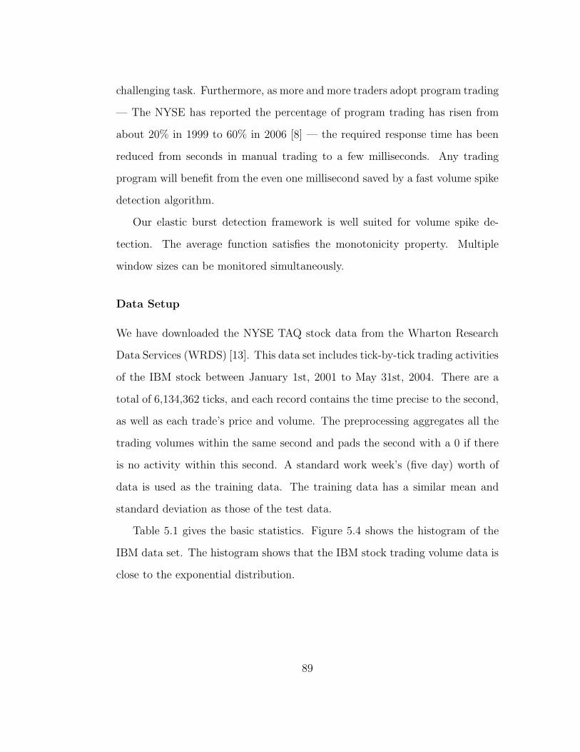
challenging task. Furthermore, as more and more traders adopt program trading

— The NYSE has reported the percentage of program trading has risen from

about 20% in 1999 to 60% in 2006 [8] — the required response time has been

reduced from seconds in manual trading to a few milliseconds. Any trading

program will benefit from the even one millisecond saved by a fast volume spike

detection algorithm.

Our elastic burst detection framework is well suited for volume spike de-

tection. The average function satisfies the monotonicity property. Multiple

window sizes can be monitored simultaneously.

Data Setup

We have downloaded the NYSE TAQ stock data from the Wharton Research

Data Services (WRDS) [13]. This data set includes tick-by-tick trading activities

of the IBM stock between January 1st, 2001 to May 31st, 2004. There are a

total of 6,134,362 ticks, and each record contains the time precise to the second,

as well as each trade’s price and volume. The preprocessing aggregates all the

trading volumes within the same second and pads the second with a 0 if there

is no activity within this second. A standard work week’s (five day) worth of

data is used as the training data. The training data has a similar mean and

standard deviation as those of the test data.

Table 5.1 gives the basic statistics. Figure 5.4 shows the histogram of the

IBM data set. The histogram shows that the IBM stock trading volume data is

close to the exponential distribution.

89

Table 5.1: Statistics for the IBM stock data

Size 23,085,000

Mean 287.06

Standard deviation 2,796.05

Min 0

Max 2,806,500

IBM Stock Data Distribution

0.00E+00

5.00E+06

1.00E+07

1.50E+07

2.00E+07

2.50E+07

Trading Volume per Second

Num

ber of T

ime P

oin

ts

IBM Stock Data Distribution

22874710

141879 34057 14647 7592 3547 1711 1277

0.00E+00

5.00E+06

1.00E+07

1.50E+07

2.00E+07

2.50E+07

1 2 3 4 5 6 7 8

Trading Volume per Second

Num

ber o

f Tim

e P

oin

ts

Figure 5.4: The histogram distribution of the IBM stock data. Each bin in

the enlarged figure stands for 5000 shares, i.e. the first bin stands for volume

0-5000, the second bin stands for volume 5000-10000, and so on.

90

CPU Time vs. Threshold - IBM

0

20

40

60

80

100

2 3 4 5 6 7 8 9 10

Burst Probability p=10-k

CP

U tim

e (s)

SBT

SAT - static

SAT - dynamic

Figure 5.5: The effect of different thresholds in the IBM data

Performance Tests

We are interested in comparing the Shifted Aggregation Tree using the static

and dynamic algorithms with the Shifted Binary Tree under different settings.

Unlike the thresholds used in the test on the synthetic data which are fixed

during the whole detection process, the thresholds used in the following tests

change dynamically based on the most recently observed data. The reason is

obvious: the thresholds set for a region with less activity can be easily exceeded

during a region with much more activity. People are usually interested in a

burst of activity relative to the most recent activity.

A burst probability p is selected to reflect the probability of a burst happen-

ing at each window size. The mean µ and standard deviation σ are computed

for each week, and used to compute the thresholds for the following week. The

threshold for window size w is set to wµ −√wσΦ−1(p), where Φ is the normal

cumulative distribution function.� Different thresholds

The thresholds are set to reflect a burst probability ranging from 10−2

91

CPU Time vs. Max Window Size of Interest - IBM

0

50

100

150

200

250

300

10 30 60 120 300 600 1800

Max Window Size of InterestC

PU

tim

e (s)

SBT

SAT - static

SAT - dynamic

Figure 5.6: The effect of different maximum window size of interest in the IBM

data

to 10−9. The maximum window size is set to 500. The task is to detect

bursts at every window size.

Figure 5.5 shows that as the burst probability decreases, the CPU time for

the Shifted Aggregation Tree decreases quickly. The Shifted Aggregation

Tree performs 3 to 4 times better than the Shifted Binary Tree. The

dynamic algorithm also performs slightly better (10 to 20 percent less

time) than the static algorithm.� Different maximum window sizes of interest

The maximum window sizes are set from 10 seconds up to 1800 seconds.

The burst probability is set to 10−6. The task is to detect bursts at every

window size.

Figure 5.6 shows the results. As the maximum window size increases,

there are more candidate levels in the desired structure, i.e. the bounding

ratio can be much more smaller compared to that in the Shifted Binary

Tree, and thus the speedup for the Shifted Aggregation Tree over the

92

CPU Time vs. Set of Window Sizes - IBM

0

5

10

15

20

25

10 30 60 120 240

Number of Window SizesC

PU

tim

e (s)

SBT

SAT - static

SAT - dynamic

Figure 5.7: The effect of different sets of window sizes of interest in the IBM

data

Shifted Binary Tree increases. Similarly, the dynamic algorithm achieves

more speedup (a factor of 1.5) as the maximum window size increases,

because adding a level of large window size can reduce the detailed search

time.� Different sets of window sizes of interest

Instead of detecting bursts at every window size, we want to see how the

Shifted Aggregation Tree performs with different sets of window sizes.

The test is performed to detect bursts for a set of n window sizes expo-

nentially evenly-spaced up to the maximum window size of interest, i.e.

{N 1

n , N2

n , N3

n , . . . , N}, where N is the maximum window size of interest.

In this test, N is set to be 3600 and n is set to be 10, 30, 60, 120, 240

respectively. The burst probability is set to be 10−6.

Figure 5.7 shows that as the set of window sizes becomes sparser, there

are fewer bursts to worry about, thus both the Shifted Binary Tree and

the Shifted Aggregation Tree take less time. As the set of window sizes

93

Table 5.2: Statistics for the test IBM data for robust test

Mean Standard deviation

IBM w12 376.21 2147.10

IBM w20 279.20 5430.01

IBM w29 401.35 2307.30

IBM w70 250.81 1716.69

IBM w100 306.83 1760.76

IBM w150 163.15 1184.95

Table 5.3: Test parameters for robust test - IBM data

Max Window Burst Number of

Size Probability Window Sizes

IBM setting1 250 10−3 250

IBM setting2 500 10−6 100

IBM setting3 750 10−7 75

IBM setting4 1000 10−8 50

becomes sparser, both the structure and the bursts become very sparse.

Thus there is little saving for the dynamic algorithm, but extra cost is

spent to check if a change is needed. The dynamic algorithm performs

slightly less well than the static algorithm in this case, taking about 10

percent more time. However, when the number of window sizes increases,

the dynamic algorithm performs better as shown in Figure 5.7.

In summary, the experiments show that this framework can handle millions

of time points and hundreds of window sizes in several seconds. The average

processing time per time point is less than 0.1 millisecond. Therefore, this

94

framework is suitable for real time processing.

Robustness test

In the static algorithm, the structure of a Shifted Aggregation Tree depends on

the input used to train it. We are interested in how sensitive the structure is

to whether training on one portion of the data gives good results when tested

on another portion, and how the dynamic algorithm performs compared to the

static algorithm.

We constructed three training sets for the IBM data. One set is taken from

the test data to be detected. The second is taken from the same type of data,

but outside the test data. For IBM, this set is taken from trading activities in

2000. The third set is taken from the other type of data, i.e, we use the SDSS

data (explained in the next section) to train a Shifted Aggregation Tree, then

use it to detect the IBM data. Each training set contains three pieces of training

data, each piece contains five days of records. Table 5.2 shows the statistics for

the training data. In the table, the first three sets are taken from the data to

be detected, the second three sets are taken outside the data to be detected.

Table 5.3 shows other parameters used in these tests.

Figure 5.8 shows the CPU times for four different test scenarios on each

training set, the CPU times for the dynamic algorithm are shown as a com-

parison. For clarity, for each setting, only one result is shown for the dynamic

algorithm starting with the structures trained with the other type of data.

When testing the structure created based on data from the same data type

but distinct from the test data, the performance of the static algorithm on the

IBM data is about the same as using a structure based on the test data itself.

The reason is that the out-of-sample training set has similar statistics to the

95

IS

OS

OT

dynam

ic

Setting1

0

5

10

15

20

25

30

35

CPU

Time

(s)

Training Set

CPU Time vs. Training Set -IBM

Setting1

Setting2

Setting3

Setting4

Figure 5.8: Robustness test on the IBM stock data (IS: in-sample, OS: out-of-

sample, OT: out-of-type)

in-sample training set. The dynamic algorithm performs better than the static

algorithm when the number of window sizes of interest is dense. However, it

performs slightly less well than the static algorithm when the number of window

sizes is sparse.

A static structure based on a different data type can perform quite poorly.

For example, a structure based on SDSS data runs 2 to 3 times slower for IBM

data than a structure based on out-of-sample IBM data. The dynamic algorithm

achieves much better performance than the static algorithm in this case. The

respective times it spent are close to those using the out-of-sample IBM data.

96

5.3 Click Fraud Detection in Website Traffic

Monitoring

As more and more businesses go online, it is critical to make their websites

attractive to customers. Website traffic monitoring and analysis plays a greater

and greater role in improving the popularity of one’s website.

One way to attract website traffic is online advertising on search engines,

such as Google or Yahoo. In this scenario, an ad is placed together with the

search results. If the visitor clicks the ad, the advertiser has to pay a small

amount of money to the search engine. This is called pay-per-click (PPC),

which has brought in billions of dollars for Google/Yahoo.

A problem that has arisen with pay-per-click is click fraud. Someone can

use an automated script or program to simulate legitimate use of a web browser

to click on an ad. This can harm the competitors by forcing them to pay more

money without bringing in real profits. Click fraud poses a serious threat to

the online advertising business. It’s difficult to capture all the frauds because

of different click behaviors.

However, one common characteristic behind click fraud is that the number

of clicks should be large enough to generate considerable money. Therefore, one

feature of click fraud can be a burst of clicks within some limited time period.

Because the automated program may generate clicks randomly, the duration

will not be known in advance, so multiple window sizes need to be monitored.

This is exactly the elastic burst detection task.

97

Table 5.4: Statistics for the SDSS SkyServer traffic data

SDSS

Size 31,536,000

Mean 120.95

Standard deviation 64.87

Min 0

Max 576

SDSS SkyServer Traffic Distribution

0

200000

400000

600000

800000

1000000

Number of Requests Per Second

Count

Figure 5.9: The histogram distribution of the Sloan Digital Sky Survey (SDSS)

SkyServer traffic data

98

Data Setup

We use the Sloan Digital Sky Survey (SDSS) SkyServer traffic data in this case

study. The Sloan Digital Sky Survey [10] SkyServer is an ambitious website

trying to make a map of a large part of the sky. This data set records all

the access traffic to the SDSS SkyServer from January 1st, 2003 to December

31st, 2003. Each record includes the request time precisely to the second, the

source IP address and the target URL. Thus this data set contains the same

information as the click data, which is also generated by browsers. The data set

has 17,432,468 records. The preprocessing aggregates all the records for each

second and places a zero in the time point entry if there is no activity within

that second. The training data consists of seven days of second-by-second data.

The basic statistics are shown in Table 5.4 and the histogram of the SDSS

data set is shown in Figure 5.9. The histogram shows that the SDSS SkyServer

traffic data follows the Poisson distribution.

Performance Tests

As for to the IBM data, we are interested in comparing the static and dynamic

detection algorithms with the Shifted Binary Tree under different settings. The

thresholds are dynamically updated based on the observed mean and standard

deviation from the previous week.� Different thresholds

The thresholds are set to reflect a burst probability ranging from 10−2

to 10−9. The maximum window size is set to 300. The task is to detect

bursts at every window size.

Figure 5.10 shows the results. Similar to its performance with the IBM

99

CPU Time vs. Threshold - SDSS

0

20

40

60

80

2 3 4 5 6 7 8 9 10

Burst Probability p=10-k

CP

U tim

e (s)

SBT

SAT - static

SAT - dynamic

Figure 5.10: The effect of different thresholds in the Sloan Digital Sky Survey

(SDSS) data

data, the static algorithm performs two to three times better than the

Shifted Binary Tree, and the dynamic algorithm performs slightly (about

1.1 times) better than the static algorithm.� Different maximum window sizes of interest

The maximum window sizes are set from 10 seconds up to 1800 seconds.

The burst probability is set to 10−6. The task is to detect bursts at every

window size.

Figure 5.11 shows results similar to those achieved with the IBM data set.

As the maximum window size increases, the speedup for the Shifted Ag-

gregation Tree over the Shifted Binary Tree increases, as does the speedup

for the dynamic algorithm over the static algorithm.� Different sets of window sizes of interest

The test is performed to detect bursts for a set of n window sizes expo-

nentially evenly-spaced up to the maximum window size of interest, i.e.

{N 1

n , N2

n , N3

n , . . . , N}, where N is the maximum window size of interest.

100

CPU Time vs. Max Window Size of Interest - SDSS

0

100

200

300

400

500

600

10 30 60 120 300 600 1800

Max Window Size of Interest

CP

U tim

e (s)

SBT

SAT - static

SAT - dynamic

Figure 5.11: The effect of different maximum window size of interest in the

Sloan Digital Sky Survey (SDSS) data

CPU Time vs. Set of Window Sizes - SDSS

0

10

20

30

40

10 30 60 120 240

Number of Window Sizes

CP

U tim

e (s)

SBT

SAT - static

SAT - dynamic

Figure 5.12: The effect of different sets of window sizes of interest in the Sloan

Digital Sky Survey (SDSS) data

101

Table 5.5: Statistics for the test SDSS data for robust test

Mean Standard deviation

SDSS w10 73.92 27.08

SDSS w18 98.84 33.24

SDSS w25 121.71 39.17

SDSS w40 168.85 50.39

SDSS w45 183.68 55.05

SDSS w50 197.58 57.57

Table 5.6: Test parameters for robust test - SDSS data

Max Window Burst Number of

Size Probability Window Sizes

SDSS setting1 200 10−4 200

SDSS setting2 400 10−5 80

SDSS setting3 600 10−6 60

SDSS setting4 800 10−8 40

N is set to be 1800 and n is set to be 10, 30, 60, 120, 240 respectively.

The burst probability is set to be 10−6.

Figure 5.12 shows the results. As for the IBM data, as the number of win-

dow sizes increases, the Shifted Aggregation Tree saves more time com-

pared to the Shifted Binary Tree. The dynamic algorithm performs about

1.5 times better than the static algorithm.

Again, the experiments show that the Shifted Aggregation Tree framework

is well suitable for real data stream environment.

102

Robustness test

We constructed three training sets for the SDSS data similar to those we con-

structed for the IBM data. One set is taken from the test data to be detected.

The second is taken from the same type of data, but from the SkyServer traffic

of 2004. The third set is taken from the IBM data. Each training set contains

three pieces of training data, each piece contains seven day’s records. Table 5.5

shows the statistics for the training data. In the table, the first three sets are

taken from the data to be detected, the second three sets are taken outside the

data to be detected. Table 5.6 shows other parameters in these tests.

Figure 5.13 shows the CPU times for four different test scenarios on each

training set, the CPU times for the dynamic algorithm are shown as a com-

parison. For clarity, for each set, only one result is shown for the dynamic

algorithm.

The in-sample training sets give similar detection times, while the out-of-

sample training sets and the out-of-type training sets take 25 percent more time.

Again, the dynamic algorithm performs better than the static algorithm when

the number of window sizes is dense.

5.4 Burst Correlation in Stock Data

We believe that high-performance burst detection could be a preliminary primi-

tive for further knowledge discovery and data mining processes. As an example,

we look at the correlation of bursts in stock data.

We collected the tick-by-tick TAQ stock data in 2003 for the Standard &

Poor’s 100 stocks. The goal is to discover which stocks share similar volume

103

IS

OS

OT

dynam

ic

Setting1

0

20

40

60

80

100

120

CPU

Time

(s)

Training Set

CPU Time vs. Training Set - SDSS

Setting1

Setting2

Setting3

Setting4

Figure 5.13: Robustness test on the Sloan Digital Survey (SDSS) traffic data

(IS: in-sample, OS: out-of-sample, OT: out-of-type)

characteristics, i.e. when there is a burst of trading in one stock, which other

stocks also exhibit a burst? Because trading bursts can happen across different

time resolutions, we monitored the correlation at multiple time scales and set

the window sizes of interest to be 10, 30, 60, and 300 seconds. The burst

probability is set to 10−9.

Bursts are detected using a Shifted Aggregation Tree, tuned as described

above. The bursts detected are converted to a 0-1 string where 0 means no

burst and 1 means a burst. The correlation is computed over these 0-1 strings.

These bursts tell an interesting story. First, stocks within the same sector are

correlated strongly e.g. Microsoft (MSFT), Oracle(ORCL) and Cisco(CSCO).

Surprisingly strong correlations of bursty behaviors can be found across different

industries also however. For example, Pfizer Inc. (PFE, health care, Drugs,

major Pharmaceuticals), Pepsico Inc. (PEP, Beverage), Procter & Gamble Co.

(PG, Non-Durables Household Products) are highly correlated. Table 5.7 shows

104

Table 5.7: Some highly-correlated stocks at different durations

Duration Highly-correlated stocks

10s C/GE/XOM, CSCO/MSFT/ORCL

30s C/GE/XOM, CSCO/MSFT/ORCL,

PEP/PFE/PG

60s C/GE/XOM/PEP/PFE/PG/GE,

CSCO/MSFT/ORCL

300s C/GE/XOM/PEP/PFE/PG/GE,

CSCO/MSFT/ORCL, WFC/XOM/WMT,

KO/USB/VZ

some highly correlated stocks at different window sizes. We are not claiming

these still anecdotal observations as a major discovery, but just as a suggestive

example of how burst detection can feed into data mining applications.

105

Chapter 6

Multi-Dimensional Elastic Burst

Detection

Real world data often have multiple attributes, for example, a demographic

data set often contains information like age, sex, profession, etc.; a geographic

information system (GIS) data set often contains latitude, longitude, the mea-

surements mapped on latitude and longitude values, etc. Bursts of events may

relate to multiple attributes, for example a disease outbreak in certain age

groups and certain professions.

In this chapter, we extend the one-dimensional elastic burst detection to D-

dimensional data. We extend the problem definition to the D-dimensional case,

then explain the changes in the data structure and the algorithm. We apply it

in an epidemiology simulation to detect disease outbreak and spread.

106

6.1 Algorithm for D-Dimensional Elastic Burst

Detection

6.1.1 Problem definition

Let S denote a D-dimensional space defined by D orthogonal axes, each axis

denoting an attribute. An event having D attributes can be seen as a point in

this D-dimensional space. Assume for attribute k, the minimum and maximum

possible values are xkmin and xk

max respectively. The whole space of interest is

the rectangle region cornered at [x1min, x

2min, . . . , x

Dmin] and [x1

max, x2max, . . . , x

Dmax].

People may be interested in bursts occurring in different regions of different

sizes in the space. For example, one may be interested in more than 5 disease

cases in a small town but more than 50 disease cases in a large city. The D-

dimensional elastic burst detection is to detect bursts of events occurring within

multiple regions of different sizes in the D-dimensional space of interest. We

use “region” instead of “window” to denote a D-dimensional space of interest.

Generally speaking, a region can be of any shape and any orientation. For

simplicity, we divide the whole D-dimensional space into many unit cells. Each

cell corresponds to a unit of minimum resolution for each attribute. This is

similar to the one-dimensional case: the incoming data are assumed to arrive

exactly at the regular time points. We consider only the number of events in

these axis-aligned rectangle regions. An axis-aligned rectangle region is defined

by its bottom most corner [x1, x2, . . . , xD] and sizes [h1, h2, . . . , hD] for each

dimension, where hi > 0.

107

6.1.2 D-dimensional Shifted Aggregation Tree

As in the one-dimensional case, a D-dimensional Shifted Aggregation Tree is

composed of several levels. The nodes at level 0 have a one-to-one correspon-

dence to the unit cells in the D-dimensional space of interest. A node at a level

above level 0 corresponds to an axis-aligned rectangular region which aggregates

all the unit cells inside this region. All nodes at the same level have the same size

and the same shifting pattern from the neighboring nodes at this level. There-

fore level k is defined by a D-dimensional region/window size [h1k, h

2k, . . . , h

Dk ]

and a D-dimensional shift [s1k, s

2k, . . . , s

Dk ].

In the one-dimensional case, for each node at level k, there are two adjacent

nodes at the same level: one before this node and another after this node.

The overlap is between two adjacent nodes. In the D-dimensional case, there

are 3D − 1 nodes adjacent to one node. The overlap is among 2D adjacent

nodes. Figure 6.1 shows how four adjacent nodes shift and overlap in the two-

dimensional case. The overlap of the adjacent nodes at the same level k is a

D-dimensional region denoted by [h1k − s1

k, h2k − s2

k, . . . , hDk − sD

k ]. Thus, all the

regions contained in the region [h1k − s1

k + 1, h2k − s2

k + 1, . . . , hDk − sD

k + 1] are

contained by a node at level k. Because of the monotonicity, if the aggregate

of a node at level k does not exceed the threshold for the size [h1k−1 − s1

k−1 +

1, h2k−1 − s2

k−1 + 1, . . . , hDk−1 − sD

k−1 + 1], there is no burst in any region of size

containing [h1k−1 − s1

k−1 + 1, h2k−1 − s2

k−1 + 1, . . . , hDk−1 − sD

k−1 + 1] but contained

by [h1k − s1

k + 1, h2k − s2

k + 1, . . . , hDk − sD

k + 1].

The D-dimensional detection algorithm is similar to the algorithm in the

one-dimensional case. The structure is updated bottom up. A detailed search

is triggered when the aggregate at a node exceeds the minimum threshold of

108

Figure 6.1: The shift and overlap between four adjacent regions (grayed) in a

two-dimensional Shifted Aggregation Tree. A grayed area represents a node.

its detailed search region. In contrast to the one-dimensional case, there is no

total order between the thresholds for the window sizes within a detailed search

region. For example, in the one-dimensional case, suppose that a detailed search

region includes window sizes from 8 to 16; due to monotonicity, the threshold for

size 8 is less than (or equal to) the threshold for size 9, and so on. In this case a

binary search is used to determine the range of the detailed search window sizes,

for example, if the aggregate is less than the threshold for size 10, there is no

need to search window sizes from 10 to 16. By contrast, in the D-dimensional

case, there is no total order between the thresholds for two window sizes, say

[9,10] and [10,9], so we cannot use binary search to determine where to start a

detailed search. Instead, we have to examine each size of interest contained in

a detailed search region for real bursts.

109

6.1.3 Adaptive D-dimensional Shifted Aggregation Tree

In the above regular D-dimensional Shifted Aggregation Tree, the nodes at each

level are over the whole space of interest. For example, in a two-dimensional

space of size [16, 16], there are 7 × 7 nodes at the level of size [4, 4] and shift

[2, 2]. In other words, the number of levels in different regions are the same. The

regular D-dimensional structure does not adapt to different data distributions

in different regions. For example, one region may have more bursts and thus

require a dense structure while another region may have fewer bursts and thus

need only a sparse structure.

An extension of this is to use different numbers of levels in different regions.

We may keep more levels in some regions than others. In other words, we can

view it as if these extra levels are missing in other regions, i.e. we only keep a

subset of the nodes at these extra levels. For example, we can keep just 3 × 3

nodes — instead of 7×7 in the regular case — at the level of size [4, 4] and shift

[2, 2], only covering one of the corners of the whole space of interest. We call

these levels partial (compared to the full levels in the regular structure), and

a structure with partial levels an adaptive D-dimensional Shifted Aggregation

Tree. Figure 6.2 shows a partial level of two nodes in a two-dimensional space

of size [6, 5], compared with the full level of four nodes as shown in Figure 6.1.

In the detection process, each node is still responsible for triggering an alarm

for its own detailed search region. In order to detect any possible burst in

the whole space of interest without any duplicate, the adaptive D-dimensional

Shifted Aggregation Tree should be constructed in such a way that the union

of all the detailed search regions partitions the whole space of interest, i.e. the

union has to cover the whole space of interest and there is no overlap between

110

Figure 6.2: A partial level in an adaptive D-dimensional Shifted Aggregation

Tree. A grayed area represents a node.

any two detailed search regions.

6.1.4 State Space Search Algorithm

Given sample data and thresholds for different window sizes, the state space

search algorithm for the D-dimensional Shifted Aggregation Tree is similar to

that for one-dimensional data. Each D-dimensional Shifted Aggregation Tree

is viewed as a state, and the growth from one tree to another is viewed as a

transformation between states. The algorithm starts with the base level of unit

size, and keeps expanding the structure by adding a level on top of the existing

structure, until the overlap region of the top level covers the maximum size of

interest. Similarly a cost is associated with each state, including the updating

cost, the filtering/checking cost and the detailed search cost. The statistics are

collected from the sample data to estimate the detailed search cost. The state

with the best cost is picked as the next state to be explored.

For the regular D-dimensional Shifted Aggregation Tree, when the structure

needs to expand, a full level is simply added to the top of the current structure,

e.g. in the above case of size [16, 16], add 7 × 7 nodes at the level of size [4, 4]

and shift [2, 2].

111

For the adaptive D-dimensional Shifted Aggregation Tree, when the struc-

ture needs to expand, a partial level is added to the top of the existing structure.

The partial level can be any subset of the full level, and can be added at differ-

ent possible subregions. For example, add 2 × 2 nodes at the level of size [4, 4]

and shift [2, 2] starting from [1, 1] to [15, 15]; or add 3 × 3 nodes starting from

[1, 1] to [14, 14]; and so on. Figure 6.3 and Figure 6.4 demonstrate the difference

between the state space growth of a regular D-dimensional Shifted Aggregation

Tree and that of an adaptive one.

6.1.5 Dynamic Detection Algorithm

In many spatial-temporal applications, spatial data changes over time. For

example, the traffic over a metro area changes depending on the working hours.

To detect bursts in a spatial-temporal data set, one can use a static D-

dimensional Shifted Aggregation Tree (either regular or adaptive) training with

a sample data set at any time point. The dynamic algorithm can be used to

adapt to changes in the data distribution in different regions.

The dynamic algorithm is similar to that in the one-dimensional case. The

following points show the difference between the D-dimensional dynamic algo-

rithm and the one-dimensional dynamic algorithm.� The structure to start with may be an adaptive D-dimensional Shifted

Aggregation Tree instead of a regular one.� When adding or deleting a level, a partial level may be added or deleted

instead of always a full level as in the one-dimensional case.� When widening or narrowing a level, there are D shifts which can be

112

Figure 6.3: State space algorithm for regular D-dimensional Shifted Aggregation

Tree in a 4 by 4 two-dimensional space. A grayed area represents a node. Nodes

grouped by the dotted lines stand for a full level. The bottom level shows the

level of unit size. The top level contains a node covering the whole space. The

middle level shows all possible full levels which can be added on top of the

bottom level.

113

Figure 6.4: State space algorithm for adaptive D-dimensional Shifted Aggrega-

tion Tree in a 4 by 4 two-dimensional space. A grayed area represents a node.

Nodes grouped by the dotted lines stand for a partial level. The bottom level

shows the level of unit size. The top level contains a node covering the whole

space. The middle levels show all possible partial levels of different sizes and

orientations at different locations, which can be added on top of the bottom

level.

114

changed. There are, in total, D2 possible shifting actions that will make

a level denser or sparser.� The shape of the alarm region may need to be changed to take into account

the spatial-temporal characteristics of the data. Remind that in the one-

dimensional case, when an alarm is raised, one may expect more alarms

soon after, i.e. alarms occur in clusters. To anticipate these alarms, we

do not make the structure sparser in the alarm region. In the multi-

dimensional case, for some data sets, the spatial distribution of the events

may change quickly from time t to t + 1, thus there may not be such a

cluster phenomenon when an alarm happens. Therefore, we may not need

alarm region from time t to t + 1.

6.2 Fast Detection of Infectious Disease Out-

break and Spread

Epidemics, such as asthma, SARS, influenza, etc., are serious threats to public

health. Epidemic outbreak detection, especially infectious disease detection, is

of great importance to aid in disease prevention and to control the spread of

diseases in their early stages. In Epidemiology, detection of disease occurrence

and discovery of the association are two important topics. Burst detection can

be a useful tool for detecting disease outbreaks. Bursts can reveal features that

suggest association or causal relations [80, 91].

In this section, we simulate the outbreak and spread of an infectious disease

and use our multi-dimensional burst detection to detect the outbreak regions.

115

Susceptible Infectious RecoveredβI γ

Figure 6.5: Susceptible-Infectious-Recovered (SIR) model

6.2.1 Mathematical Models in Epidemiology

Epidemiologists have used different mathematical models to model the outcome

and spread of infectious diseases [45]. The classic model used in infectious

disease modeling is the SIR model as shown in Figure 6.5. In the basic SIR

model, the whole population is divided into three classes depending on their

experience with respect to the disease. S denotes the susceptible population

who have never been infected by the disease and are subject to the infection.

Once infected, they change to the I class, denoting the population infected by

the disease and will stay in this class for the whole infectious period. When

recovered, they change to the R class, denoting the population who recovered

from the disease and are assumed to be immune for life. Figure 6.5 demonstrates

the relationship between these three groups. β is the contact rate, denoting the

contact degree between the susceptible and the infectious. γ is the recovery

rate, denoting how fast the infected recover.

The whole progress of the disease infection without birth and death can be

modeled by the following ordinary differential equations:

dS

dt= −βIS

dI

dt= βIS − γI

dR

dt= γI

116

where S(t), I(t) and R(t) are the size of the population in each class respectively,

and the constants are positive.

The basic SIR model does not consider the movement of the population.

In the real world, people often spread disease when they travel. The epidemic

metapopulation model is an extension to the basic SIR model to take population

movement into consideration [92].

The metapopulation theory was developed in ecology to study the interaction

between populations of the same species distributed in fragmented and isolated

locations. The epidemic metapopulation model makes an analogy between the

dynamics of ecological metapopulations and the dynamics of infectious diseases.

It uses the basic SIR model to compute the sizes of the S, I and R classes for each

location. Instead of assuming the population at each location is constant, the

spatial movement between different locations is taken into consideration. The

population at each location fluctuates based on the movement dynamics between

different locations. A simple way to model the movement rate between locations

is to use the inverse of the distance between these two locations: the closer two

locations, the more movements. A more reasonable method, as described in

[92], is to consider the sizes of the populations at these two locations as well:

the larger the population of the two locations, the more movements between

them.

6.2.2 Simulation

We use the epidemic metapopulation model described above to simulate how

an infectious disease would break out and spread in a geographical region after

an initial case is detected. We use the tri-state area (New York, New Jersey

117

and Connecticut) as the spatial region of interest for demonstration in this

simulation. The simulation is done over a month-long period to see how a disease

would start and spread in the tri-state area. After the number of infectious is

computed for each location, two-dimensional burst detection is used to discover

the regions with the most serious disease outbreak.

Data Setup

We obtain the population data for the tri-state area from the U.S. Census Bu-

reau [12] and the transportation data from the Bureau of Transportation Statis-

tics [3]. Instead of using the population sizes to compute the movement rate,

we use the real transportation data explicitly to quantify the spatial interaction

between different locations.

The population data comes from the 2000 census. It contains the summary

population at each county-subdivision (i.e. town) level. There are, in total,

about 1900 subdivisions in the tri-state area. Figure 6.6 shows the population

distribution.

The transportation data includes the passenger travel census data of the

tri-state area in 2000. The Census Transportation Planning Package (CTPP)

2000 includes the detailed Journey-To-Work statistics about the commute from

home to work. The number of the workers going from the residence to the work

place is counted for each possible pair of residence-workplaces. The statistics

are per town, i.e. at the same resolution as the population data. We interpret

the number of workers as a population movement from the residence to the

workplace in the morning and in the opposite direction at night. So the indi-

vidual population at each location fluctuates, but the overall population stays

the same.

118

Figure 6.6: Population distribution of the Tri-State area. The darker an area,

the denser the population.

119

Disease outbreak and spread detection

Given the population data and the transportation data, we simulate the out-

break and spread process of an infectious disease in the following steps:

1. A town is picked as the initial place where one disease case is detected,

say Queens.

2. For each day, the following revised SIR model is used to compute the

number of S, I and R for each town i.

dSi

dt=

∑

j

(−βIjSij)

dIi

dt=

∑

j

(βIjSij) − γIi

dRi

dt= γIi

where Sij is the number of susceptible people traveling between town i

and town j. The number of newly infected in town i is the sum of the

number of newly infected who traveled to other towns and got infected

there, plus those newly infected by the infectious in this town. We assume

the infectious people do not go to work or travel.

3. After computing the number of the infected in each town, the numbers are

mapped to a 128× 128 grid which covers the whole region. For simplicity

and clarity, the bursts are detected across only 3 window sizes of square

regions in this simulation: 1 by 1, 4 by 4 and 8 by 8 respectively. Realistic

applications may require a finer-resolution grid and more window sizes of

different shapes and different orientations.

120

In this simulation, the contact ratio β is set to be 0.0001, and the recovery

rate γ is set to be 0.33. The thresholds are set to reflect a burst probability of

0.00001. Figures [6.7,6.8, 6.9,6.10,6.11] show a sequence of detected outbreak

regions every 6 days. The regions with wave, brick and dot patterns stand for

square regions of size 8 by 8, 4 by 4 and 1 by 1 respectively. It shows that

starting in Queens, the disease soon spreads to Manhattan. Because there is a

large population flow from Manhattan to the tri-state area, the disease spreads

along all routes to NJ, upstate NY and CT. Quick burst detection enables us

to quickly monitor and respond to the spread of a disease or a bioterror attack.

121

Figure 6.7: Simulation of a disease spread and outbreak detection - Day 1

122

Figure 6.8: Simulation of a disease spread and outbreak detection - Day 7

123

Figure 6.9: Simulation of a disease spread and outbreak detection - Day 13

124

Figure 6.10: Simulation of a disease spread and outbreak detection - Day 19

125

Figure 6.11: Simulation of a disease spread and outbreak detection - Day 25

126

Chapter 7

Conclusion

In this thesis, we have proposed an efficient algorithmic framework for the elastic

burst detection problem. This framework includes a family of data structures

and a static algorithm to train an efficient structure given a small sample of input

data, and further a greedy dynamic algorithm which dynamically changes the

structure to adapt to the incoming data. We tested our framework extensively

on different types of data and different parameter settings. The experiments

show that our method outperforms the existing method over a variety of inputs.

We applied our framework in several real world applications in physics, finance,

website/network traffic monitoring, etc. We also extend this work to multi-

dimensional data and apply it in an epidemiology simulation to efficiently detect

disease outbreak and spread.

127

Bibliography

[1] Adaptive dataflow for querying streams and deep web and beyond.

http://telegraph.cs.berkeley.edu/.

[2] The aurora project. http://www.cs.brown.edu/research/aurora/.

[3] Bureau of transportation statistics. http://www.transtats.bts.gov.

[4] Hubble space telescope website. http://hubblesite.org/.

[5] Maids overview. http://maids.ncsa.uiuc.edu/about/index.html.

[6] Market volume analysis. http://marketvolume.com/.

[7] Milagro gamma-ray observatory. http://www.lanl.gov/milagro/.

[8] New york stock exchange. http://nyse.com/.

[9] Niagara query engine. http://www.cs.wisc.edu/niagara.

[10] Sloan digital sky survey. http://www.sdss.org/.

[11] Stanford stream data manager. http://www-db.stanford.edu/stream/.

[12] U.s. census bureau. http://www.census.gov.

128

[13] Wharton research data services (wrds).

http://wrds.wharton.upenn.edu/.

[14] C. C. Aggarwal, J. Han, J. Wang, and P. S. Yu. A framework for clustering

evolving data streams. In Proceedings of 29th International Conference on

Very Large Data Bases, pages 81–92, 2003.

[15] C. C. Aggarwal, J. Han, J. Wang, and P. S. Yu. A framework for pro-

jected clustering of high dimensional data streams. In Proceedings of 30th

International Conference on Very Large Data Bases, pages 852–863, 2004.

[16] C. C. Aggarwal, J. Han, J. Wang, and P. S. Yu. On demand classification of

data streams. In Proceedings of the 10th ACM SIGKDD International Con-

ference on Knowledge Discovery and Data Mining, pages 503–508, 2004.

[17] C. C. Aggarwal and P. S. Yu. Outlier detection for high-dimensional data.

In Proceedings of the 2001 ACM SIGMOD International Conference on

Management of Data, pages 37–46, 2001.

[18] B. Babcock, S. Babu, M. Datar, R. Motwani, and J. Widom. Models and

issues in data stream systems. In Proceedings of 21st ACM Symposium on

Principles of Database Systems, pages 1–16, 2002.

[19] B. Babcock, M. Datar, R. Motwani, and L. O’Callaghan. Maintaining

variance and k-medians over data stream windows. In Proceedings of the

22nd Symposium on Principles of Database Systems, pages 234–243, 2003.

[20] S. Babu and J. Widom. Continuous queries over data streams. In Proceed-

ings of the 2001 ACM SIGMOD International Conference on Management

of Data, pages 109–120, 2001.

129

[21] V. Barnett and T. Lewis. Outliers in Statistical Data. John Wiley & Sons,

1994.

[22] S. D. Bay and M. Schwabacher. Mining distance-based outliers in near

linear time with randomization and a simple pruning rule. In Proceedings of

the 9th ACM SIGKDD International Conference on Knowledge Discovery

and Data Mining, pages 29–38, 2003.

[23] M. Breuing, H.-P. Kriegel, P. Kroger, and J. Sander. Data bubbles: Quality

preserving performance boosting for hierarchical clustering. In Proceedings

of the 2001 ACM SIGMOD International Conference on Management of

Data, pages 79–90, 2001.

[24] M. M. Breunig, H.-P. Krigel, R. T. Ng, and J. Sander. Lof: Identifying

density-based local outliers. In Proceedings of the 2000 ACM SIGMOD

International Conference on Management of Data, pages 93–104, 2000.

[25] Y. D. Cai, D. Clutter, G. Pape, J. Han, M. Welge, and L. Auvil. Maids:

Mining alarming incidents from data streams. In Proceedings of the 2004

ACM SIGMOD International Conference on Management of Data, pages

919–920, 2004.

[26] K. Chakrabarti and S. Mehrotra. Locally dimensionality reduction: A

new approach to indexing high dimensional spaces. In Proceedings of the

6th ACM SIGKDD International Conference on Knowledge Discovery and

Data Mining, pages 89–100, 2000.

130

[27] Y. Chen, G. Dong, J. Han, B. W. Wah, and J. Wang. Multi-dimensional

regression analysis of time series data streams. In Proceedings of 28th

International Conference on Very Large Data Bases, pages 323–334, 2002.

[28] R. Cole, D. Shasha, and X. Zhao. Fast window correlations over uncoopera-

tive time series. In Proceeding of the eleventh ACM SIGKDD international

conference on Knowledge discovery in data mining, pages 743–749. ACM

Press, 2005.

[29] M. Datar, A. Gionis, P. Indyk, and R. Motwani. Maintaining stream statis-

tics over sliding windows: (extended abstract). In Proceedings of the thir-

teenth annual ACM-SIAM symposium on Discrete algorithms, pages 635–

644. Society for Industrial and Applied Mathematics, 2002.

[30] V. de Silva and J. B. Tenenbaum. Global versus local methods in nonlinear

dimensionality reduction. pages 705–712. Advances in Neural Information

Processing Systems, 2002.

[31] C. Ding, X. He, H. Zha, and H. D. Simon. Adaptive dimension reduction

for clustering high dimensional data. In Proceedings of the 2002 IEEE

International Conference on Data Mining, pages 147–154, 2002.

[32] A. Dobra, M. Garofalakis, J. Gehrke, and R. Rastogi. Processing complex

aggregate queries over data streams. In Proceedings of the 2002 ACM

SIGMOD International Conference on Management of Data, pages 61–72,

2002.

131

[33] P. Domingos and G. Hulten. Mining high-speed data streams. In Pro-

ceedings of the 6th ACM SIGKDD International Conference on Knowledge

Discovery and Data Mining, pages 71–80, 2000.

[34] G. Dong, J. Han, L. V. Lakshmanan, J. Pei, H. Wang, and P. S.Yu. Online

mining of changes from data streams: Research problems and preliminary

results. In Proceedings of the 2003 ACM SIGMOD International Confer-

ence on Management of Data, 2003.

[35] W. DuMouchel, C. Volinsky, T. johnson, C. Cortes, and D. Pregibon.

Squashing flat files flatter. In Proceedings of the 5th ACM SIGKDD In-

ternational Conference on Knowledge Discovery and Data Mining, pages

6–15, 1999.

[36] C. Faloutsos. Indexing and mining streams. In Proceedings of the 2004

ACM SIGMOD International Conference on Management of Data, page

969, 2004.

[37] S. Ganguly, M. Garofalakis, and R. Rastogi. Processing data-stream join

aggregates using skimmed sketches. pages 569–586. International Confer-

ence on Extending Database Technology (EDBT), 2004.

[38] M. Garofalakis, J. Gehrke, and R. Rastogi. Querying and mining data

streams: You only get one look. In Proceedings of the 2002 ACM SIGMOD

International Conference on Management of Data, page 635, 2002.

[39] V. Geobel and T. Plagemann. Data stream management systems - con-

cepts, prototypes, and applications. Multimedia Interactive Protocols and

Systems, 2004.

132

[40] P. B. Gibbons and S. Tirthapura. Distributed stream algorithms for sliding

windows. In Proceedings of the fourteenth annual ACM symposium on

Parallel algorithms and architectures, pages 63–72, 2002.

[41] L. Golab and M. T. Ozsu. Issues in data stream management. ACM

SIGMOD Record, 32(2):5–14, 2003.

[42] M. Greenwald and S. Khanna. Space-efficient online computation of quan-

tile summaries. In Proceedings of the 2001 ACM SIGMOD international

conference on Management of data, pages 58–66. ACM Press, 2001.

[43] D. Gunopulos and G. Das. Time series similarity measures and time se-

ries indexing. In Proceedings of the 2001 ACM SIGMOD International

Conference on Management of Data, page 624, 2001.

[44] S. Heiler. A survey on nonparametric time series analy-

sis. Finance 9904005, EconWPA, Apr. 1999. available at

http://ideas.repec.org/p/wpa/wuwpfi/9904005.html.

[45] H. W. Hethcote. The mathematics of infectious diseases. Society for In-

dustrial and Applied Mathematics Review, 42:599–653, 2000.

[46] P. Indyk, N. Koudas, and S. Muthukrishnan. Identifying representative

trends in massive time series data sets using sketches. In Proceedings of the

26th International Conference on Very Large Data Bases, pages 363–372.

Morgan Kaufmann Publishers Inc., 2000.

[47] Y. E. Ioannidis and V. Poosala. Histogram-based approximation of set-

valued query answers. In Proceedings of 25th International Conference on

Very Large Data Bases, pages 174–185, 1999.

133

[48] T. Johnson, I. Kwok, and R. Ng. Fast computation of 2-dimensional depth

contour. In Proceedings of the 4th ACM SIGKDD International Conference

on Knowledge Discovery and Data Mining, 1998.

[49] E. Keogh. A tutorial on indexing and mining time series data. In Proceed-

ings of the 2001 IEEE International Conference on Data Mining, 2001.

[50] E. Keogh, K. Chakrabarti, S. Mehrotra, and M. Pazzani. Locally adap-

tive dimensionality reduction for indexing large time series databases. In

Proceedings of the 2001 ACM SIGMOD International Conference on Man-

agement of Data, pages 151–162, 2001.

[51] E. Keogh, K. Chakrabarti, M. Pazzani, and S. Mehrotra. Dimensionality

reduction for fast similarity search in large time series database. pages

263–286. Databases and Knowledge and Information Systems, 2000.

[52] E. Keogh and S. Kasetty. On the need for time series data mining bench-

marks: A survey and empirical demonstration. In Proceedings of the

6th ACM SIGKDD International Conference on Knowledge Discovery and

Data Mining, pages 349–371, 2000.

[53] E. Keogh, S. Lonardi, and W. Chiu. Finding surprising patterns in a time

series database in linear time and space. In Proceedings of the 8th ACM

SIGKDD International Conference on Knowledge Discovery and Data Min-

ing, pages 550–556, 2002.

[54] E. Keogh and M. J. Pazzani. An enhanced representation of time series

which allows fast and accurate classification, clustering and relevance feed-

134

back. In Proceedings of the 4th ACM SIGKDD International Conference

on Knowledge Discovery and Data Mining, pages 239–243, 1998.

[55] J. Kleinberg. Bursty and hierarchical structure in streams. In Proceed-

ings of the Eighth ACM SIGKDD International Conference on Knowledge

Discovery and Data Mining, pages 91–101. ACM Press, 2002.

[56] E. M. Knorr, R. T. Ng, , and V. Tucakov. Distance-based outliers: Algo-

rithms and applications. In Proceedings of 26th International Conference

on Very Large Data Bases, pages 237–253, 2000.

[57] E. M. Knorr and R. T. Ng. Algorithms for mining distance-based outliers

in large datasets. In Proceedings of 24th International Conference on Very

Large Data Bases, pages 392–403, 1998.

[58] E. M. Knorr and R. T. Ng. Finding intensional knowledge of distance-

based outliers. In Proceedings of 25th International Conference on Very

Large Data Bases, pages 211–222, 1999.

[59] A. Lerner, D. Shasha, Z. Wang, X. Zhao, and Y. Zhu. Fast algorithms

for time series with applications to finance and physics and music and

biology and and other suspects. In Proceedings of the 2004 ACM SIGMOD

International Conference on Management of Data, pages 965–968, 2004.

[60] X.-B. Li. Data reduction via adaptive sampling. Communication in Infor-

mation and System, 2002.

[61] J. Lin, E. Keogh, S. Lonardi, and B. Chiu. A symbolic representation of

time series, with implications for streaming algorithms. In Proceedings of

135

the 8th ACM SIGMOD workshop on Research issues in data mining and

knowledge discovery, pages 2–11. ACM Press, 2003.

[62] J. Ma and S. Perkins. Online novelty detection on temporal sequences. In

Proceedings of the 9th ACM SIGKDD International Conference on Knowl-

edge Discovery and Data Mining, pages 613–618, 2003.

[63] J. Ma and S. Perkins. Time series novelty detection using one-class support

vector machines. International Joint Conference on Neural Networks, 2003.

[64] S. Madden, M. Shah, J. M. Hellerstein, and V. Raman. Continuously

adaptive continuous queries over streams. In Proceedings of the 2002 ACM

SIGMOD International Conference on Management of Data, pages 49–60,

2002.

[65] G. S. Manku and R. Motwani. Approximate frequency counts over data

streams. In Proceedings of 28th International Conference on Very Large

Data Bases, pages 356–357, 2002.

[66] Y. Matias, J. S. Vitter, and M. Wang. Wavelet-based histograms for selec-

tivity estimation. In Proceedings of the 1998 ACM SIGMOD International

Conference on Management of Data, pages 448–459, 1998.

[67] Y. Matias, J. S. Vitter, and M. Wang. Dynamic maintenance of wavelet-

based histograms. In Proceedings of 26th International Conference on Very

Large Data Bases, pages 101–110, 2000.

[68] D. C. Montgomery and G. C. Runger. Applied Statistics and Probability

for Engineers. Wiley, 2003.

136

[69] D. Neill and A. Moore. Rapid detection of significant spatial clusters. In

Proceedings of the 10th ACM SIGKDD International Conference on Knowl-

edge Discovery and Data Mining, 2004.

[70] D. Neill and A. Moore. Anomalous spatial cluster detection. In Proceed-

ings of the KDD 2005 Workshop on Data Mining Methods for Anomaly

Detection, August 2005.

[71] D. B. Neill and A. W. Moore. A fast multi-resolution method for detection

of significant spatial disease clusters. In S. Thrun, L. Saul, and B. Scholkopf,

editors, Advances in Neural Information Processing Systems 16. MIT Press,

2004.

[72] D. B. Neill, A. W. Moore, F. Pereira, and T. Mitchell. Detecting significant

multidimensional spatial clusters. In L. K. Saul, Y. Weiss, and L. Bottou,

editors, Advances in Neural Information Processing Systems 17, pages 969–

976. MIT Press, 2005.

[73] N. J. Nilsson. Principles of Artificial Intelligence. Morgan Kaufmann

Publishers, 1980.

[74] S. Papadimitriou and C. Faloutsos. Adaptive and hands-off streaming min-

ing. In Proceedings of 29th International Conference on Very Large Data

Bases, pages 560–571, 2003.

[75] S. Papadimitriou and C. Faloutsos. Cross-outlier detection. pages 199–213.

8th International Symposium on Spatial and Temporal Databases, 2003.

137

[76] S. Papadimitriou, H. Kitagawa, P. B. Gibbons, and C. Faloutsos. Loci:

Fast outlier detection using the local correlation integral. In Proceedings of

the 19th International Conference on Data Engineering, page 315, 2003.

[77] C.-S. Perng, H. Wang, S. R. Zhang, and D. S. Parker. Landmarks: a

new model for similarity-based pattern querying in time series databases.

In Proceedings of the 16th International Conference on Data Engineering,

pages 33–42, 2000.

[78] L. Qiao, D. Agrawal, and A. E. Abbadi. Rhist: Adaptive summarization

over continuous data streams. pages 469–476. Conference on Information

and Knowledge Management, 2002.

[79] S. Russell and P. Norvig. Artificial Intelligence: A Modern Approach.

Prentice Hall, 2002.

[80] R. Sabhnani, D. Neill, and A. Moore. Detecting anomalous patterns in

pharmacy retail data. In Proceedings of the KDD 2005 Workshop on Data

Mining Methods for Anomaly Detection, August 2005.

[81] S. Schaal, S. Vijayakumar, and C. G. Atkeson. Local dimensionality re-

duction. Advances in Neural Information Processing Systems, 1997.

[82] B. Scholkopf, R. Williamson, A. smola, J. Shawe-Tayleor, and J. Platt.

Support vector method for novelty detection. pages 582–588. Advances in

Neural Information processing Systems 12, 1999.

[83] C. Shahabi, X. Tian, and W. Zhao. Tsa-tree: A wavelet-based approach

to improve the efficiency of multi-level surprise and trend queries on time-

138

series data. pages 1–14. 12th International Conference on Scientific and

Statistical Database Management(SSDBM), 2000.

[84] D. Shasha and Y. Zhu. High Performance Discovery in Time Series: Tech-

niques and Case Studies, pages 151–172. Springer, 2004.

[85] L. Shih, J. D. Rennie, Y.-H. Chang, and D. R. Karger. Text bundling:

Statistics-based data reduction. pages 696–703. International Conference

on Machine Learning, 2003.

[86] R. Typke, F. Wiering, and R. C. Veltkamp. A survey of music information

retrieval systems. In ISMIR 2005, 6th International Conference on Music

Information Retrieval, pages 153–160, 2005.

[87] M. Vlachos, C. Meek, Z. Vagena, and D. Gunopulos. Identifying similar-

ities, periodicities and bursts for online search queries. In Proceedings of

the 2004 ACM SIGMOD international conference on Management of data,

pages 131–142. ACM Press, 2004.

[88] H. Wang, W. Fan, P. S. Yu, and J. Han. Mining concept-drifting data

streams using ensemble classifiers. In Proceedings of the 9th ACM SIGKDD

International Conference on Knowledge Discovery and Data Mining, pages

226–235, 2003.

[89] M. Wang, T. Madhyastha, N. H. Chan, S. Papadimitriou, and C. Faloutos.

Data mining meets performance evaluation: Fast algorithms for modeling

bursty traffic. In ICDE ’02: Proceedings of the 18th International Con-

ference on Data Engineering (ICDE’02), pages 507–516. IEEE Computer

Society, 2002.

139

[90] W. Willinger, M. S. Taqqu, and A. Erramilli. A bibliographical guide to

self-similar traffic and performance modeling for modern high-speed net-

works. 1996.

[91] W.-K. Wong, A. Moore, G. Cooper, and M. Wagner. Bayesian network

anomaly pattern detection for disease outbreaks. In Proceedings of the

Twentieth International Conference on Machine Learning, pages 808–815.

AAAI Press, August 2003.

[92] Y. Xia, O. N. Bjrnstad, and B. T. Grenfell. Measles metapopulation dy-

namics: A gravity model for epidemiological coupling and dynamics. The

American Naturalist, 164:267–281, 2004.

[93] T. Zhang, R. Ramakrishnan, and M. Linvy. Birch: An efficient data clus-

tering method for very large databases. In Proceedings of the 1996 ACM

SIGMOD International Conference on Management of Data, pages 103–

114, 1996.

[94] X. Zhang and D. Shasha. High performance burst detection. Technical

Report, New York University, 2005.

[95] X. Zhang and D. Shasha. Better burst detection. In Proceedings of the

22nd International Conference on Data Engineering (ICDE’06), page 146.

IEEE Computer Society, 2006.

[96] X. Zhao, X. Zhang, T. Neylon, and D. Shasha. Incremental methods for

simple problems in time series: Algorithms and experiments. In 9th In-

ternational Database Engineering & Application Symposium, pages 3–14,

2005.

140

[97] C. Zhu, H. Kitagawa, S. Papadimitri, and C. Faloutsos. Obe: Outlier by

example. pages 222–234. Pacific-Asia Conference on Knowledge Discovery

and Data Mining, 2004.

[98] Y. Zhu and D. Shasha. Statstream: Statistical monitoring of thousands of

data streams in real time. In Proceedings of 28th International Conference

on Very Large Data Bases, pages 358–369, 2002.

141