FAPP07 ism 04 - University of Wisconsin–Madison

55

Chapter 4 Linear Programming

Chapter Outline Introduction Section 4.1 Mixture Problems: Combining Resources to Maximize Profit Section 4.2 Finding the Optimal Production Policy Section 4.3 Why the Corner Point Principle Works Section 4.4 Linear Programming: Life Is Complicated Section 4.5 A Transportation Problem: Delivering Perishables Section 4.6 Improving on the Current Solution Chapter Summary A fundamental management problem that a company faces is determining how much of each of its products to produce in order to maximize profit. This problem is called a mixture problem, and linear programming is a powerful technique used to solve such problems. To get started, we must know certain information about the mixture problem:

• what products are to be made • what resources will be needed • how much of each resource is available • how much of each resource is used by each product • how much profit is generated by each unit of each product

The variables in the problem are the number of units of each product produced. They are assumed to be nonnegative (minimum constraints). A production policy is a specification of how many units of each product are to be made. To be achievable, a production policy has to satisfy the natural constraints of the problem, since no policy can use more of a resource than the company has available. Production policies satisfying all problem constraints are called feasible solutions to the problem, and the set of all feasible solutions is called the feasible region.

The profit function is an expression built from the variables and per-unit profits that tell us how much profit is produced by a given feasible solution. To solve our mixture problem, we need to find a feasible solution that produces the largest possible profit. Linear programming applies in the case when the problem constraints are linear inequalities and the profit function is linear in the variables. In this case, the feasible region is polygonal in 2-space and polyhedral in 3-space. It will have an analogous structure in higher dimensions.

The geometry of this situation is crucial to the solution. A fundamental result, the corner point principle, states that the optimal solution occurs at a corner of the feasible region. This result suggests a possible solution strategy.

• find all corners of the feasible region • determine the profit at each corner point • choose the production policy of any corner producing the maximum profit

56 Chapter 4

Computationally, this procedure suffers from the same problem as the brute force method applied to the TSP; for large problems there are just too many corners to check quickly. Fortunately, faster algorithms exist to solve linear programming problems. The simplex method developed by George Dantzig starts at some corner of the feasible region and then moves from corner to neighboring corner, always going to a corner where profit is the same or larger, until it locates a corner producing maximum profit. An alternative to the simplex method is Karmarker’s algorithm, which bores into the interior of the feasible region to decide which corner to examine next. The simplex method is fast in practice but can be shown no more efficient than the brute force method on certain cleverly constructed problems. Karmarker’s algorithm provides a computationally efficient method for solving linear programming problems.

In the transportation problem, we are interested in meeting demands while minimizing cost. Information can be set up in a tableau. The tableau shows costs and rim conditions for the transporation problem. Using the Northwest Corner Rule (NCR), we can obtain a feasible solution. This solution, however, may not be optimal. By calculating and comparing the values of indicator cells, we can improve on the feasible solution. Using the stepping stone method, we look at indicator cells that have negative values and determine an optimal solution.

Skill Objectives 1. Create a chart to represent the given information in a linear programming problem with two

variables.

2. From its associated chart, write the constraints of a linear programming problem as linear inequalities.

3. List two implied constraints in every linear programming problem.

4. Formulate a profit equation for a linear-programming problem when given the per-unit profits.

5. Describe the graphical implications of the implied constraints 0x ≥ and 0.y ≥

6. Draw the graph of a line in a coordinate-axis system.

7. Graph a linear inequality in a coordinate-axis system.

8. Determine by a substitution process whether a point with given coordinates is contained in the graph of a linear inequality.

9. Indicate the feasible region for a linear programming problem by shading the graphical intersection of its constraints.

10. Locate the corner points of a feasible region from its graph.

11. Evaluate the profit function at each corner point of a feasible region.

12. Apply the corner point theorem to determine the maximum profit for a linear programming problem.

13. Interpret the corner point producing the maximum profit as the solution to the corresponding linear programming problem.

14. List two methods for solving linear programming problems with many variables.

15. Given a tableau, apply the Northwest Corner Rule to find a feasible solution.

16. Calculate the cost of the system found by the Northwest Corner Rule.

17. Calculate the value of indicator cells.

18. Use the stepping stone method to find an optimal solution.

Linear Programming 57

Teaching Tips

1. The material differs significantly from that in other texts. The basic ideas are introduced one at a time; first, mixture problems having just one resource, then resource constraints are added, followed by minimum quantities for products and, finally, two products and two resources. Along the way, the students are introduced to the profit function, making mixture charts, the feasible region, and the corner principle. Although this approach is nonstandard, the slow buildup of ideas enables students to comprehend the material more thoroughly.

2. Because many of the students taking this course have only an algebra background, a review of coordinate graphing is often helpful. This is especially true when graphing linear inequalities. The concept of selecting a test point often requires additional explanation.

3. A short review of the concept of set intersection may be helpful when indicating the feasible region on a linear programming graph.

4. The instructor will need to decide whether to require the student to find the intersection point of two boundary lines by solving a system of linear equations, or to have the coordinates of that point provided to the student. Requiring the solution will probably necessitate reviewing that procedure in class discussion.

5. When setting up the chart for a linear programming problem, you may want to interchange the rows and columns in the text example. If the variables name the columns and the resources the rows, then the inequalities can be written easily from the chart in a horizontal fashion. This may be easier for the student because of its visual simplicity.

6. When graphing several linear inequalities, students find it helpful to have colored pens or pencils to indicate the different half-planes. It is then easier to find the feasible region because the intersection is the region that contains all the colors.

7. Text Exercises 30–41 offer a variety of settings for linear programming problems. These can be used to advantage in working through examples with students.

8. You may choose to prepare in advance blank tableaux for students to use during lecture of applying the Northwest Corner Rule to find a feasible solution.

Research Paper In this chapter, two methods for solving linear programming problems with many variables are briefly discussed. These are the simplex method and Karmarkar’s algorithm. Prior to Karmarkar’s algorithm (1984), Leonid Khaciyan presented a method guaranteeing to solve any linear programming problem in 1979. Students can further investigate these methods and their origins, discuss their similarities and differences, or prepare a general discussion of the contributions of these two mathematicians.

58 Chapter 4

Collaborative Learning

Linear Programming

You live on a farm and bake chocolate chip cookies and chocolate chip muffins in your home, and sell them to the public. One morning, you check your supplies and discover that you are low on flour and chocolate chips, but have plenty of the other ingredients. Your car is in the repair shop and there are 2 feet of snow on the ground, so there is no way to replenish your supplies until tomorrow.

Each batch of cookies requires 2 pounds of flour and 1 pound of chocolate chips; each batch of muffins uses 3 pounds of flour and 2 pounds of chocolate chips. You have 60 pounds of flour and 36 pounds of chocolate chips on hand.

Your profit on each batch of cookies is $8, and on muffins your profit is $13 per batch. How should you divide your baking between cookies and muffins in order to maximize your profit for the day?

Hints:

a. If no cookies are baked, how many batches of muffins can be baked? What will the profit be in this case?

b. Answer the same questions if no muffins are baked.

c. Which is more profitable: baking only cookies or only muffins?

d. Is there a mix of cookies and muffins that makes even more money than either only muffins or only cookies?


Solutions Skills Check:

1. a 2. c 3. b 4. b 5. b 6. c 7. c 8. c 9. b 10. c

11. b 12. c 13. c 14. c 15. c 16. c 17. c 18. a 19. a 20. c

Exercises: 1. (a) 2 3 12x y+ =

y-intercept: Substitute 0.x =

( )

123

2 0 3 12

0 3 12

3 12 4

y

y

y y

+ =

+ == ⇒ = =

y-intercept is ( )0,4 .

x-intercept: Substitute 0.y =

( )

122

2 3 0 12

2 0 12

2 12 6

x

x

x x

+ =

+ == ⇒ = =

x-intercept is ( )6,0 .

Graph:

(b) 3 5 30x y+ =


( )

305

3 0 5 30

0 5 30

5 30 6

y

y

y y

+ =

+ == ⇒ = =



( )

303

3 5 0 30

3 0 30

3 30 10

x

x

x x

+ =

+ == ⇒ = =


Graph:

(c) 4 3 24x y+ =


( )

243

4 0 3 24

0 3 24

3 24 8

y

y

y y

+ =

+ == ⇒ = =



( )

244

4 3 0 24

4 0 24

4 24 6

x

x

x x

+ =

+ == ⇒ = =


Graph:

Continued on next page

60 Chapter 4

1. continued

(d) 7 4 42x y+ =


( )

424

7 0 4 42

0 4 42

4 42 10.5

y

y

y y

+ =

+ == ⇒ = =

y-intercept is ( )0,10.5 .


( )

427

7 4 0 42

7 0 42

7 42 6

x

x

x x

+ =

+ == ⇒ = =


Graph:

(e) 3x = − This form represents a vertical line. y-intercept: None x-intercept: ( )3,0 .−

Graph:

(f) 6y =

This form represents a horizontal line. y-intercept is ( )0,6 . x-intercept: None

Graph:

2. (a) 4 3 18x y+ = and 0x =

Note: This situation is shown only for the first quadrant. The y-intercept of 4 3 18x y+ = can be found by substituting 0.x =

( )183

4 0 3 18

0 3 18 3 18 6

y

y y y

+ =

+ = ⇒ = ⇒ = =

The y-intercept is ( )0,6 .

The x-intercept of 4 3 18x y+ = can be found by substituting 0.y =

( )184

4 3 0 18

4 0 18 4 18 4.5

x

x x x

+ =

+ = ⇒ = ⇒ = =

The x-intercept is ( )4.5,0 .

0x = represents a vertical line, namely the y-axis.



2. (a) continued To find the point of intersection, substitute 0x = into 4 3 18.x y+ =

( )

183

4 0 3 18

0 3 18

3 18 6

y

y

y y

+ =+ =

= ⇒ = =

The point of intersection is therefore ( )0,6 .

(b) 5 3 45x y+ = and 5y = −

Note: This situation is shown only for the first and fourth quadrants. The y-intercept of 5 3 45x y+ = can be found by substituting 0.x =

( )

453

5 0 3 45

0 3 45

3 45 15

y

y

y y

+ =+ =

= ⇒ = =



( )

455

5 3 0 45

5 0 45

5 45 9

x

x

x x

+ =+ =

= ⇒ = =

The x-intercept is ( )9,0 .

5y = − represents a horizontal line, which lies below the x-axis.

To find the point of intersection, substitute 5y = − into 5 3 45.x y+ =

( )( )

605

5 3 5 45

5 15 45

5 15 45

5 60 12

x

x

x

x x

+ − =

+ − =

− == ⇒ = =

The point of intersection is therefore ( )12, 5 .−

62 Chapter 4

3. Note: These situations are shown only for the first quadrant.

(a) 10x y+ = and 2 14x y+ =

The y-intercept of 10x y+ = can be found by substituting 0.x =

0 10

10

y

y

+ ==


The x-intercept of 10x y+ = can be found by substituting 0.y =

0 10

10

x

x

+ ==


The y-intercept of 2 14x y+ = can be found by substituting 0.x =

142

0 2 14

2 14

7

y

y

y

+ === =


The x-intercept of 2 14x y+ = can be found by substituting 0.y =

( )2 0 14

0 14

14

x

x

x

+ =

+ ==


To find the point of intersection, we can multiply both sides of 10x y+ = by 1,− and add

the result to 2 14.x y+ =

10

2 14

4

x y

x y

y

− − = −+ =

=

Substitute 4y = into 10x y+ = to solve to x.

4 10 6x x+ = ⇒ =




3. continued

(b) 2 0y x− = and 4x =

4x = represents a vertical line, which lies to the right of the y-axis.

By substituting either 0x = or 0,y = we see that 2 0y x− = passes through ( )0,0 , the

origin. By substituting an arbitrary value (except 0) for one of the variables, we can find another point that lies on the graph of 2 0.y x− = Since we see the point of intersection

with the graph of 4,x = we could use this value.

( )2 4 0

8 0

8

y

y

y

− =

− ==

Thus, a second point on the graph of 2 0y x− = is ( )4,8 . This is also the point of

intersection between the two lines.

4. Note: These situations are shown only for the first quadrant. (a) 8x ≥

The graph of 8x = represents a vertical line with x-intercept ( )8,0 . Since any value of x to

the right of this line is greater than 8, we shade the portion to the right of this vertical line.

(b) 5y ≥

The graph of 5y = represents a horizontal line with y-intercept ( )0,5 . Since any value of y

above this line is greater than 5, we shade the portion above this horizontal line.


64 Chapter 4

4. continued (c) 5 3 15x y+ ≤

The y-intercept of 5 3 15x y+ = can be found by substituting 0.x =

( ) 1535 0 3 15 0 3 15 3 15 5y y y y+ = ⇒ + = ⇒ = ⇒ = =



( ) 1555 3 0 15 5 0 15 5 15 3x x x x+ = ⇒ + = ⇒ = ⇒ = =


We draw a line connecting these points. Testing the point ( )0,0 , we have the statement

( ) ( )5 0 3 0 15+ ≤ or 0 15.≤ This is a true statement, thus we shade the half-plane

containing our test point, the down side of the line.

(d) 4 5 30x y+ ≤


( ) 3054 0 5 30 0 5 30 5 30 6y y y y+ = ⇒ + = ⇒ = ⇒ = =



( ) 3044 5 0 30 4 0 30 4 30 7.5x x x x+ = ⇒ + = ⇒ = ⇒ = =






5. Note: These situations are shown only for the first quadrant. (a) 4x ≥

The graph of 4x = represents a vertical line with x-intercept ( )4,0 . Since any value of x to

the right of this line is greater than 4, we shade the portion to the right of this vertical line.

(b) 9y ≥

The graph of 9y = represents a horizontal line with y-intercept ( )0,9 . Since any value of y

above this line is greater than 9, we shade the portion above this horizontal line.

(c) 3 2 18x y+ ≤


( ) 1823 0 2 18 0 2 18 2 18 9y y y y+ = ⇒ + = ⇒ = ⇒ = =



( ) 1833 2 0 18 3 0 18 3 18 6x x x x+ = ⇒ + = ⇒ = ⇒ = =






66 Chapter 4

5. continued (d) 7 2 42x y+ ≤


( ) 4227 0 2 42 0 2 42 2 42 21y y y y+ = ⇒ + = ⇒ = ⇒ = =



( ) 4277 2 0 42 7 0 42 7 42 6x x x x+ = ⇒ + = ⇒ = ⇒ = =





6. (a) 2 4 28x y+ ≤

(b) ( )( )

2 0.5 40 pruning

0.5 0.25 2 shredding

x y

x y

+ ≤

+ ≤

7. (a) 6 4 300x y+ ≤

(b) 30 72 420x y+ ≤

8. ( )( )

12 10 640 beef

4 3 480 pork

x y

x y

+ ≤

+ ≤

9. 0; 0; 2 12x y x y≥ ≥ + ≤

The constraints of 0 and 0x y≥ ≥ indicate that we are restricted to the upper right quadrant

created by the x-axis and y-axis. The y-intercept of 2 12x y+ = can be found by substituting 0.x =

1220 2 12 2 12 6y y y+ = ⇒ = ⇒ = =



( )2 0 12 0 12 12x x x+ = ⇒ + = ⇒ =



( )0 2 0 12+ ≤ or 0 12.≤ This is a true statement, thus we shade the half-plane containing our

test point, the down side of the line, which is contained in the upper right quadrant.


10. 0; 0; 2 10x y x y≥ ≥ + ≤



( )2 0 10 0 10 10y y y+ = ⇒ + = ⇒ =


The x-intercept of 2 10x y+ = can be found by substituting 0.y = 1022 0 10 2 10 5x x x+ = ⇒ = ⇒ = =



( )2 0 0 10+ ≤ or 0 10.≤ This is a true statement, thus we shade the half-plane containing our

test point, the down side of the line, which is contained in the upper right quadrant.

11. 0; 0; 2 5 60x y x y≥ ≥ + ≤


created by the x-axis and y-axis. The y-intercept of 2 5 60x y+ = can be found by substituting 0.x =

( ) 6052 0 5 60 0 5 60 12y y y+ = ⇒ + = ⇒ = =



( ) 6022 5 0 60 2 0 60 2 60 30x x x x+ = ⇒ + = ⇒ = ⇒ = =



( ) ( )2 0 5 0 60+ ≤ or 0 60.≤ This is a true statement, thus we shade the half-plane containing

our test point, the down side of the line, which is contained in the upper right quadrant.

68 Chapter 4

12. 10; 0; 3 5 120x y x y≥ ≥ + ≤

The constraints of 10 and 0x y≥ ≥ indicate that we are restricted to the upper right quadrant, to

the right of the vertical line 10.x = The point of intersection between 10x = and 3 5 120x y+ = can be found by substituting 10x =

into 3 5 120.x y+ =

( ) 9053 10 5 120 30 5 120 5 90 18y y y y+ = ⇒ + = ⇒ = ⇒ = =

Thus, the point of intersection is ( )10,18 .


( ) 12053 0 5 120 0 5 120 24y y y+ = ⇒ + = ⇒ = =



( ) 12033 5 0 120 3 0 120 3 120 40x x x x+ = ⇒ + = ⇒ = ⇒ = =




our test point, the down side of the line, which is contained in the upper right quadrant to the right of the vertical line 10.x =


13. 0; 4; 20x y x y≥ ≥ + ≤

The constraints of 0 and 4x y≥ ≥ indicate that we are restricted to the upper right quadrant,

above the horizontal line 4.y =

The point of intersection between 4y = and 20x y+ = can be found by substituting 4y = into

20.x y+ =

4 20 16x x+ = ⇒ =



0 20 20y y+ = ⇒ =



0 20 20x x+ = ⇒ =



0 0 20+ ≤ or 0 20.≤ This is a true statement, thus we shade the half-plane containing our test point, the down side of the line, which is contained in the upper right quadrant above the horizontal line 4.y =

70 Chapter 4

14. 2; 6; 3 2 30x y x y≥ ≥ + ≤


the right of the vertical line 2x = and above the horizontal line 6.y =

The point of intersection between 2x = and 6y = is ( )2,6 .

The point of intersection between 2x = and 3 2 30x y+ = can be found by substituting 2x =

into 3 2 30.x y+ =

( ) 2423 2 2 30 6 2 30 2 24 12y y y y+ = ⇒ + = ⇒ = ⇒ = =


The point of intersection between 6y = and 3 2 30x y+ = can be found by substituting 6y =

into 3 2 30.x y+ =

( ) 1833 2 6 30 3 12 30 3 18 6x x x x+ = ⇒ + = ⇒ = ⇒ = =



( ) 3023 0 2 30 0 2 30 2 30 15y y y y+ = ⇒ + = ⇒ = ⇒ = =



( ) 3033 2 0 30 3 0 30 3 30 10x x x x+ = ⇒ + = ⇒ = ⇒ = =




our test point, the down side of the line, which is contained in the upper right quadrant to the right of the vertical line 2x = and above the horizontal line 6.y =


15. For Exercise 9: 0; 0; 2 12x y x y≥ ≥ + ≤

( )2, 4 : Since 2 0,≥ the constraint 0x ≥ is satisfied.

Since 4 0,≥ the constraint 0y ≥ is satisfied.

Since ( )2 2 4 2 8 10 12,+ = + = ≤ the condition 2 12x y+ ≤ is satisfied.

Thus, ( )2, 4 is feasible.

( )10,6 : Since 10 0,≥ the constraint 0x ≥ is satisfied.


Since ( )10 2 6 10 12 22 12,+ = + = > the condition 2 12x y+ ≤ is not satisfied.

Thus, ( )10,6 is not feasible.

For Exercise 11: 0; 0; 2 5 60x y x y≥ ≥ + ≤



Since ( ) ( )2 2 5 4 4 20 24 60,+ = + = ≤ the condition 2 12x y+ ≤ is satisfied.




Since ( ) ( )2 10 5 6 20 30 50 60,+ = + = ≤ the condition 2 12x y+ ≤ is satisfied.

Thus, ( )10,6 is feasible.

For Exercise 13: 0; 4; 20x y x y≥ ≥ + ≤



Since 2 4 6 20,+ = ≤ the condition 20x y+ ≤ is satisfied.

Thus, ( )2, 4 is feasible. Note: It is on the boundary.




Thus, ( )10,6 is feasible.

16. For Exercise 10: 0; 0; 2 10x y x y≥ ≥ + ≤



Since ( )2 2 4 4 4 8 10,+ = + = ≤ the condition 2 10x y+ ≤ is satisfied.







72 Chapter 4

16. continued


( )2, 4 : Since 2 10,< the constraint 10x ≥ is not satisfied.

Thus, ( )2, 4 is not feasible. Note: There is no need to check the other constraints.



Since ( ) ( )3 10 5 6 30 30 60 120,+ = + = ≤ the condition 3 5 120x y+ ≤ is satisfied.

Thus, ( )10,6 is feasible. Note: It is on the boundary.



Since 4 6,< the constraint 6y ≥ is not satisfied.

Thus, ( )2, 4 is not feasible. Note: There is no need to check the other constraint.



Since ( ) ( )3 10 2 6 30 12 42 30,+ = + = > the condition 3 2 30x y+ ≤ is not satisfied.


17. We wish to maximize $2.30 $3.70 .x y+

Corner Point Value of the Profit Formula: $2.30 $3.70x y+

( )( )( )

0,0

0,30

12,0

( ) ( )( ) ( )

( ) ( )

$2.30 0 $3.70 0 $0.00 $0.00 $0.00

$2.30 0 $3.70 30 $0.00 $111.00 $111.00*

$2.30 12 $3.70 0 $27.60 $0.00 $27.60

+ = + =+ = + =+ = + =

Optimal production policy: Make 0 skateboards and 30 dolls for a profit of $111.

18. We wish to maximize $5.50 $1.80 .x y+


( )( )( )

0,0

0,30

12,0

( ) ( )( ) ( )

( ) ( )

$5.50 0 $1.80 0 $0.00 $0.00 $0.00

$5.50 0 $1.80 30 $0.00 $54.00 $54.00

$5.50 12 $1.80 0 $66.00 $0.00 $66.00*

+ = + =+ = + =+ = + =

Optimal production policy: Make 12 skateboards and 0 dolls for a profit of $66.


19. Note: These situations are shown only for the first quadrant. (a) 5 4 22x y+ = and 5 10 40x y+ =


( )

224

5 0 4 22

0 4 22

4 22

5.5

y

y

y

y

+ =

+ === =

The y-intercept is ( )0,5.5 .


( )

225

5 4 0 22

5 0 22

5 22

4.4

x

x

x

x

+ =

+ === =



( )

4010

5 0 10 40

0 10 40

4

y

y

y

+ =

+ == =



( )

404

5 10 0 40

5 0 40

5 40

8

x

x

x

x

+ =

+ === =


To find the point of intersection, we can multiply both sides of 5 4 22x y+ = by 1,− and

adding the result to 5 10 40.x y+ =

186

5 4 22

5 10 40

6 18 3

x y

x y

y y

− − = −+ =

= ⇒ = =

Substitute 3y = into 5 10 40x y+ = and solve for x.

( ) 1055 10 3 40 5 30 40 5 10 2x x x x+ = ⇒ + = ⇒ = ⇒ = =



74 Chapter 4

19. continued (b) 7x y+ = and 3 4 24x y+ =


0 7

7

y

y

+ ==



0 7

7

x

x

+ ==



( )

244

3 0 4 24

0 4 24

6

y

y

y

+ =

+ == =



( )

243

3 4 0 24

3 0 24

3 24

8

x

x

x

x

+ =

+ === =


To find the point of intersection, we can multiply both sides of 7x y+ = by 3,− and adding

the result to 3 4 24x y+ =

3 3 21

3 4 24

3

x y

x y

y

− − = −+ =

=

Substitute 3y = into 3 4 24x y+ = and solve for x.

( ) 1233 4 3 24 3 12 24 3 12 4x x x x+ = ⇒ + = ⇒ = ⇒ = =



20. 0; 0; 3 9; 2 8x y x y x y≥ ≥ + ≤ + ≤



( )3 0 9 0 9 9y y y+ = ⇒ + = ⇒ =





( )3 0 0 9+ ≤ or 0 9.≤ This is a true statement.

The y-intercept of 2 8x y+ = can be found by substituting 0.x = 820 2 8 2 8 4y y y+ = ⇒ = ⇒ = =



( )2 0 8 0 8 8x x x+ = ⇒ + = ⇒ =




Thus, we shade the part of the plane in the upper right quadrant which is on the down side of both the lines 3 9x y+ = and 2 8x y+ = .

Three of the corner points, ( ) ( )0,0 , 0, 4 , and ( )3,0 lie on the coordinate axes. The fourth

corner point is the point of intersection between the lines 3 9x y+ = and 2 8x y+ = . We can

find this by multiplying both sides of 3 9x y+ = by 2,− and adding the result to 2 8.x y+ =

105

6 2 18

2 8

5 10 2

x y

x y

x x −−

− − = −+ =

− = − ⇒ = =

Substitute 2x = into 2 8x y+ = and solve for y. 622 2 8 2 6 3y y y+ = ⇒ = ⇒ = =


76 Chapter 4

21. 0; 0; 2 4;4 4 12x y x y x y≥ ≥ + ≤ + ≤



( )2 0 4 0 4 4y y y+ = ⇒ + = ⇒ =







( ) 1244 0 4 12 0 4 12 3y y y+ = ⇒ + = ⇒ = =



( ) 1244 4 0 12 4 0 12 4 12 3x x x x+ = ⇒ + = ⇒ = ⇒ = =



( ) ( )4 0 4 0 12+ ≤ or 0 12.≤ This is a true statement.

Thus, we shade the part of the plane in the upper right quadrant which is on the down side of both the lines 2 4x y+ = and 4 4 12x y+ = .

Three of the corner points, ( ) ( )0,0 , 0,3 , and ( )2,0 lie on the coordinate axes. The fourth

corner point is the point of intersection between the lines 2 4x y+ = and 4 4 12x y+ = . We can

find this by multiplying both sides of 2 4x y+ = by 4,− and adding the result to 4 4 12.x y+ =

44

8 4 16

4 4 12

4 4 1

x y

x y

x x −−

− − = −+ =

− = − ⇒ = =

Substitute 1x = into 2 4x y+ = and solve for y.

( )2 1 4 2 4 2y y y+ = ⇒ + = ⇒ =



22. 0; 2; 5 14; 2 10x y x y x y≥ ≥ + ≤ + ≤

The constraints of 0 and 2x y≥ ≥ indicate that we are restricted to the upper right quadrant,

above the horizontal line 2.y =


( )5 0 14 0 14 14y y y+ = ⇒ + = ⇒ =


The x-intercept of 5 14x y+ = can be found by substituting 0.y = 1455 0 14 5 14 2.8x x x+ = ⇒ = ⇒ = =




The y-intercept of 2 10x y+ = can be found by substituting 0.x = 1020 2 10 2 10 5y y y+ = ⇒ = ⇒ = =



( )2 0 10 0 10 10x x x+ = ⇒ + = ⇒ =




Thus, we shade the part of the plane in the upper right quadrant which is on the down side of both the lines 5 14x y+ = and 2 10x y+ = , which is also above the horizontal line 2.y =

Two of the corner points, ( )0,2 and ( )0,5 , lie on the coordinate axes. The third corner point is

the point of intersection between the lines 5 14x y+ = and 2y = . We can find this by

substituting 2y = into 5 14x y+ = to solve for y. We have 1255 2 14 5 12 2.4.x x x+ = ⇒ = ⇒ = =

The point of intersection is therefore ( )2.4,2 .

The fourth corner point is the point of intersection between the lines 5 14x y+ = and

2 10x y+ = . We can find this by multiplying both sides of 5 14x y+ = by 2,− and adding the

result to 2 10.x y+ =

189

10 2 28

2 10

9 18 2

x y

x y

x x −−

− − = −+ =

− = − ⇒ = =

Substitute 2x = into 2 10x y+ = and solve for y. We have 822 2 10 2 8 4.y y y+ = ⇒ = ⇒ = =

The point of intersection is therefore ( )2, 4 .

78 Chapter 4

23. 4; 0; 5 4 60; 13x y x y x y≥ ≥ + ≤ + ≤


the right of the vertical line 4.x = The y-intercept of 5 4 60x y+ = can be found by substituting 0.x =

( ) 6045 0 4 60 0 4 60 15y y y+ = ⇒ + = ⇒ = =



( ) 6055 4 0 60 5 0 60 5 60 12x x x x+ = ⇒ + = ⇒ = ⇒ = =



( ) ( )5 0 4 0 60+ ≤ or 0 60.≤ This is a true statement.


0 13 13y y+ = ⇒ =



0 13 13x x+ = ⇒ =



0 0 13+ ≤ or 0 13.≤ This is a true statement. Thus, we shade the part of the plane in the upper right quadrant which is on the down side of both the lines 5 4 60x y+ = and 13,x y+ = which is also to the right of the vertical line 4.x =

Two of the corner points, ( )4,0 and ( )12,0 , lie on the coordinate axes. The third corner point is

the point of intersection between the lines 13x y+ = and 4x = . We can find this by

substituting 4x = into 13x y+ = to solve to y. We have, 4 13 9.y y+ = ⇒ = The point of

intersection is therefore ( )4,9 .

The fourth corner point is the point of intersection between the lines 5 4 60x y+ = and

13.x y+ = We can find this by multiplying both sides of 13x y+ = by 4,− and adding the

result to 5 4 60.x y+ =

4 4 52

5 4 60

8

x y

x y

x

− − = −+ =

=

Substitute 8x = into 13x y+ = and solve for y. We have 8 13 5.y y+ = ⇒ = The point of



24. For Exercise 21: 0; 0; 2 4;4 4 12x y x y x y≥ ≥ + ≤ + ≤




There is no need to check the fourth constraint. Thus, ( )4, 2 is not feasible.




There is no need to check the fourth constraint. Thus, ( )1,3 is not feasible.

For Exercise 23: 4; 0; 5 4 60; 13x y x y x y≥ ≥ + ≤ + ≤



Since ( ) ( )5 4 4 2 20 8 28 60,+ = + = ≤ the condition 5 4 60x y+ ≤ is satisfied.



( )1,3 : Since 1 4,< the constraint 4x ≥ is not satisfied.

There is no need to check the other three constraints. Thus, ( )1,3 is not feasible.

25. Maximize 3 2P x y= + subject to 3; 2; 10;2 3 24x y x y x y≥ ≥ + ≤ + ≤

We need to first graph the feasible region while finding the corner points. The constraints of 3 and 2x y≥ ≥ indicate that we are restricted to the upper right quadrant, to


The point of intersection between 3x = and 2y = is ( )3, 2 .


0 10 10y y+ = ⇒ =



0 10 10x x+ = ⇒ =



( ) 2432 0 3 24 0 3 24 3 24 8y y y y+ = ⇒ + = ⇒ = ⇒ = =



( ) 2422 3 0 24 2 0 24 2 24 12x x x x+ = ⇒ + = ⇒ = ⇒ = =



80 Chapter 4

25. continued Testing the point ( )0,0 in both 10x y+ ≤ and 2 3 24,x y+ ≤ we have the following.

( ) ( )0 0 0 10 and 2 0 3 0 0 24+ = ≤ + = ≤

Since these are both true statements, we shade the down side of the line of both lines which is contained in the upper right quadrant to the right of the vertical line 3x = and above the horizontal line 2.y =


into 2 3 24.x y+ = We have ( ) 1832 3 3 24 6 3 24 3 18 6.y y y y+ = ⇒ + = ⇒ = ⇒ = = Thus, the

point of intersection is ( )3,6 .


10.x y+ = We have, 2 10 8.x x+ = ⇒ = Thus, the point of intersection is ( )8, 2 .

The final corner point is the point of intersection between 10x y+ = and 2 3 24.x y+ = We can

find this by multiplying both sides of 10x y+ = by 2,− and adding the result to 2 3 24.x y+ =

2 2 20

2 3 24

4

x y

x y

y

− − = −+ =

=

Substitute 4y = into 10x y+ = and solve for x. We have, 4 10 6.x x+ = ⇒ = The point of


We wish to maximize 3 2 .P x y= +

Corner Point Value of the Profit Formula: 3 2x y+

( )( )( )( )

3,6

3,2

8,2

6,4

( ) ( )( ) ( )( )( )

( )( )

3 3 2 6 9 12 21

3 3 2 2 9 4 13

3 8 2 2 24 4 28*

18 8 263 6 2 4

+ = + =+ = + =

+ = + =+ = + =

The maximum value occurs at the corner point ( )8,2 , where P is equal to 28.


26. Maximize 3 2P x y= − subject to 2; 3; 3 18;6 4 48x y x y x y≥ ≥ + ≤ + ≤



The point of intersection between 2x = and 3y = is ( )2,3 .


( )3 0 18 0 18 18y y y+ = ⇒ + = ⇒ =





( ) 4846 0 4 48 0 4 48 4 48 12y y y y+ = ⇒ + = ⇒ = ⇒ = =



( ) 4866 4 0 48 6 0 48 6 48 8x x x x+ = ⇒ + = ⇒ = ⇒ = =


Testing the point ( )0,0 in both 3 18x y+ ≤ and 6 4 48,x y+ ≤ we have the following.

( ) ( ) ( )3 0 0 0 18 and 6 0 4 0 0 48+ = ≤ + = ≤

Since these are both true statements, we shade the down side of the line of both lines which is contained in the upper right quadrant to the right of the vertical line 2x = and above the horizontal line 3.y =


into 6 4 48.x y+ = We have, ( ) 3646 2 4 48 12 4 48 4 36 9.y y y y+ = ⇒ + = ⇒ = ⇒ = = Thus, the

point of intersection is ( )2,9 .

The point of intersection between 3y = and 3 18x y+ = can be found by substituting 3y = into

3 18.x y+ = We have 1533 3 18 3 15 5.x x x+ = ⇒ = ⇒ = = Thus, the point of intersection is

( )5,3 .

The final corner point is the point of intersection between 3 18x y+ = and 6 4 48.x y+ = We

can find this by multiplying both sides of 3 18x y+ = by 4,− and adding the result to

6 4 48.x y+ =

246

12 4 72

6 4 48

6 24 4

x y

x y

x x −−

− − = −+ =

− = − ⇒ = =

Substitute 4x = into 3 18x y+ = and solve for y. We have, ( )3 4 18 12 18 6.y y y+ = ⇒ + = ⇒ =



82 Chapter 4

26. continued

We wish to maximize 3 2 .P x y= −

Corner Point Value of the Profit Formula: 3 2x y−

( )( )( )( )

2,3

5,3

4,6

2,9

( ) ( )( ) ( )( )( )

( )( )

3 2 2 3 6 6 0

3 5 2 3 15 6 9*

3 4 2 6 12 12 0

6 18 123 2 2 9

− = − =− = − =

− = − =− = − = −


27. Maximize 5 2P x y= + subject to 2; 4; 10x y x y≥ ≥ + ≤



The point of intersection between 2x = and 4y = is ( )2, 4 .


0 10 10y y+ = ⇒ =



0 10 10x x+ = ⇒ =


Testing the point ( )0,0 in 10,x y+ ≤ we have the following.

0 0 0 10+ = ≤ Since this is a true statement, we shade the down side of this line which is contained in the upper right quadrant to the right of the vertical line 2x = and above the horizontal line 4.y =

The point of intersection between 2x = and 10x y+ = can be found by substituting 2x = into

10.x y+ = We have 2 10 8.y y+ = ⇒ = Thus, the point of intersection is ( )2,8 .


10.x y+ = We have 4 10 6.x x+ = ⇒ = Thus, the point of intersection is ( )6,4 .



27. continued

We wish to maximize 5 2 .P x y= +


( )( )( )

2, 4

2,8

6,4

( ) ( )( ) ( )( ) ( )

5 2 2 4 10 8 18

5 2 2 8 10 16 26

5 6 2 4 30 8 38*

+ = + =+ = + =+ = + =


28. (a) 0; 0; 7 4 13x y x y≥ ≥ + ≤


created by the x-axis and y-axis. The y-intercept of 7 4 13x y+ = can be found by substituting 0.x =

( ) 1347 0 4 13 0 4 13 4 13y y y y+ = ⇒ + = ⇒ = ⇒ =

The y-intercept is ( )1340, . For graphing purposes, treat 13

4 as 143 .


( ) 1377 4 0 13 7 0 13 7 13x x x x+ = ⇒ + = ⇒ = ⇒ =

The x-intercept is ( )137 ,0 . For graphing purposes, treat 13

7 as 671 .



containing our test point, the down side of the line, which is contained in the upper right quadrant.


84 Chapter 4

28. continued

(b) According to the optimal production policy, we are looking for the maximum of 21 11 ,P x y= + given our constraints.


( )( )( )

134

137

0,0

0,

,0

( ) ( )( ) ( )( ) ( )

13 143 34 4 4

137

21 0 11 0 0 0 0

21 0 11 0 35

21 11 0 39 0 39*

+ = + =+ = + =

+ = + =

The maximum value occurs at the corner point ( )137 ,0 .

29. (a) The optimal corner point for Exercise 28 being ( )137 ,0 , the coordinates of ( )2,0 .Q =

(b) ( )2,0 is not a feasible point.

(c) The profit at ( )2,0 is greater than the profit at ( )137 ,0 .

(d) Since 0 0≥ and 3 0≥ the constraints 0x ≥ and 0y ≥ are satisfied, respectively. Also,

since ( ) ( )7 0 4 3 0 12 12 13,+ = + = ≤ the constraint 7 4 13x y+ ≤ is satisfied. Thus,

( )0,3R = is feasible. The profit at R is ( ) ( )21 0 11 3 33.+ = This is less than the profit at Q.

(e) Solving maximization problems involving linear constraints but where the variables are required to take on integer values cannot be solved by first solving the associated linear programming problem and rounding the answer to the nearest integers. This example shows the rounded value used to obtain an integer solution may not be feasible. Even if the rounded value is feasible it may not be optimal. "Integer programming" is unfortunately a much harder problem to solve than linear programming.

For Exercises 30 – 41, part (e) (using a simplex algorithm program) will not be addressed in the solutions.

30. (a) Let x be the number of shirts and y be the number of vests.

Cloth (600 yds) Minimums Profit

Shirts, x items 3 100 $5

Vests, y items 2 30 $2

(b) Profit formula: $5 $2P x y= +

Constraints: ( ) ( )100 and 30 minimums ;3 2 600 clothx y x y≥ ≥ + ≤

(c) Feasible region:



30. continued Corner points: One corner point is the point of intersection between 100 and 30x y= = ,

namely ( )100,30 . Another is the point of intersection between 100 and 3 2 600.x x y= + =

Substituting 100 into 3 2 600,x x y= + = we have the following.

( )3 100 2 600 300 2 600 2 300 150y y y y+ = ⇒ + = ⇒ = ⇒ =

Thus, ( )100,150 is the second corner point. The third corner point is the point of

intersection between 30 and 3 2 600.y x y= + = Substituting 30 into 3 2 600,y x y= + = we

have the following.

( )3 2 30 600 3 60 600 3 540 180x x x x+ = ⇒ + = ⇒ = ⇒ =

Thus, ( )180,30 is the third corner point.

(d) We wish to maximize $5 $2 .x y+

Corner Point Value of the Profit Formula: $5 $2x y+

( )( )( )

100,30

100,150

180,30

( ) ( )( ) ( )( ) ( )

$5 100 $2 30 $500 $60 $560

$5 100 $2 150 $500 $300 $800

$5 180 $2 30 $900 $60 $960*

+ = + =+ = + =+ = + =

Optimal production policy: Make 180 shirts and 30 vests.

With zero minimums, the feasible region looks like the following.

We wish to maximize $5 $2 .x y+


( )( )( )

0,0

0,300

200,0

( ) ( )( ) ( )

( ) ( )

$5 0 $2 0 $0 $0 $0

$5 0 $2 300 $0 $600 $600

$5 200 $2 0 $1000 $0 $1000*

+ = + =+ = + =+ = + =

The production policy changes to make 200 shirts and no vests.

86 Chapter 4

31. (a) Let x be the number of oil changes and y be the number tune-ups.

Time (8,000 min) Minimums Profit

Oil changes, x 20 0 $15 Tune-ups, y 100 0 $65


Constraints: ( ) ( )0 and 0 minimums ;20 100 8,000 timex y x y≥ ≥ + ≤


Corner points: The corner points are intercepts on the axes. These are ( )0,0 , ( )0,80 , and

( )400,0 .



( )( )

( )

0,0

0,80

400,0

( ) ( )( ) ( )

( ) ( )

$15 0 $65 0 $0 $0 $0

$15 0 $65 80 $0 $5200 $5200

$15 400 $65 0 $6000 $0 $6000*

+ = + =+ = + =+ = + =

Optimal production policy: Schedule 400 oil changes and no tune-ups. With non-zero minimums, the constraints are as follows.

( ) ( )50 and 20 minimums ;20 100 8,000 timex y x y≥ ≥ + ≤

The feasible region looks like the following.

Corner points: One corner point is the point of intersection between 50 and 20x y= = , namely

( )50, 20 . Another is the point of intersection between 50 and 20 100 8000.x x y= + =


( )20 50 100 8000 1000 100 8000 100 7000 70y y y y+ = ⇒ + = ⇒ = ⇒ =

Thus, ( )50,70 is the second corner point. The third corner point is the point of intersection

between 20 and 20 100 8000.y x y= + = Substituting 20 into 20 100 8000,y x y= + = we have

the following.

( )20 100 20 8000 20 2000 8000 20 6000 300x x x x+ = ⇒ + = ⇒ = ⇒ =




31. continued We wish to maximize $15 $65 .x y+


( )( )

( )

50, 20

50,70

300,20

( ) ( )( ) ( )

( ) ( )

$15 50 $65 20 $750 $1300 $2050

$15 50 $65 70 $750 $4550 $5300

$15 300 $65 20 $4500 $1300 $5800*

+ = + =+ = + =+ = + =

Optimal production policy: Schedule 300 oil changes and 20 tune-ups.

32. (a) Let x be the number of minutes processing mail orders and y be the number of minutes processing voice-mail orders.

Time (90 min) Minimums Profit

Mail order, x minutes 10 0 $30 Voice-mail order, y minutes 15 0 $40


Constraints: ( ) ( )0 and 0 minimums ;10 15 90 timex y x y≥ ≥ + ≤



( )9,0 .



( )( )( )

0,0

0,6

9,0

( ) ( )( ) ( )( ) ( )

$30 0 $40 0 $0 $0 $0

$30 0 $40 6 $0 $240 $240

$30 9 $40 0 $270 $0 $270*

+ = + =+ = + =+ = + =

Optimal production policy: Process 9 mail orders and no voice-mail orders.


88 Chapter 4

32. continued With non-zero minimums, the constraints are ( ) ( )3 and 2 minimums ;10 15 90 time .x y x y≥ ≥ + ≤



( )3, 2 . Another is the point of intersection between 3 and 10 15 90.x x y= + = Substituting

3 into 10 15 90x x y= + = we have the following.

( )10 3 15 90 30 15 90 15 60 4y y y y+ = ⇒ + = ⇒ = ⇒ =

Thus, ( )3, 4 is the second corner point. The third corner point is the point of intersection

between 2 and 10 15 90.y x y= + = Substituting 2 into 10 15 90y x y= + = we have the

following.

( )10 15 2 90 10 30 90 10 60 6x x x x+ = ⇒ + = ⇒ = ⇒ =




( )( )( )

3,2

3,4

6,2

( ) ( )( ) ( )( ) ( )

$30 3 $40 2 $90 $80 $170

$30 3 $40 4 $90 $160 $250

$30 6 $40 2 $180 $80 $260*

+ = + =+ = + =+ = + =

Optimal production policy: Process 6 mail orders and 2 voice-mail orders.

33. (a) Let x be the number of routine visits and y be the number of comprehensive visits.

Doctor Time (1800 min) Minimums Profit

Routine, x visits 5 0 $30 Comprehensive, y visits 25 0 $50






33. (c) continued Corner points: The corner points are intercepts on the axes. These are ( )0,0 , ( )0,72 , and

( )360,0 .



( )( )( )

0,0

0,72

360,0

( ) ( )( ) ( )

( ) ( )

$30 0 $50 0 $0 $0 $0

$30 0 $50 72 $0 $3600 $3600

$30 360 $50 0 $10,800 $0 $10,800*

+ = + =+ = + =+ = + =

Optimal production policy: Schedule 360 routine visits and no comprehensive visits. With non-zero minimums, the constraints are as follows.

( ) ( )20 and 30 minimums ;5 25 1800 timex y x y≥ ≥ + ≤



( )20,30 . Another is the point of intersection between 20 and 5 25 1800.x x y= + = Substituting

20 into 5 25 1800,x x y= + = we have the following.

( )5 20 25 1800 100 25 1800 25 1700 68y y y y+ = ⇒ + = ⇒ = ⇒ =


between 30 and 5 25 1800.y x y= + = Substituting 30 into 5 25 1800,y x y= + = we have the

following.

( )5 25 30 1800 5 750 1800 5 1050 210x x x x+ = ⇒ + = ⇒ = ⇒ =




( )( )

( )

20,30

20,68

210,30

( ) ( )( ) ( )

( ) ( )

$30 20 $50 30 $600 $1500 $2100

$30 20 $50 68 $600 $3400 $4000

$30 210 $50 30 $6300 $1500 $7800*

+ = + =+ = + =+ = + =

Optimal production policy: Schedule 210 routine visits and 30 comprehensive visits.

34. (a) Let x be the number of loaves of multigrain bread and y be the number of loaves of herb bread.

Breads (600 loaves) Minimums Profit

Multigrain, x loaves 1 100 $8 Herb, y loaves 1 200 $10


Constraints: ( ) ( )100 and 200 minimums ; 600 breadsx y x y≥ ≥ + ≤


90 Chapter 4

34. continued (c) Feasible region:

Corner points: One corner point is the point of intersection between 100 and 200x y= = ,

namely ( )100,200 . Another is the point of intersection between 100 and 600.x x y= + =

Substituting 100 into 600,x x y= + = we have the following.

100 600 500y y+ = ⇒ =

Thus, ( )100,500 is the second corner point. The third corner point is the point of

intersection between 200 and 600.y x y= + = Substituting 200 into 600,y x y= + = we

have the following. 200 600 400x x+ = ⇒ =




( )( )( )

100,200

100,500

400,200

( ) ( )( ) ( )( ) ( )

$8 100 $10 200 $800 $2000 $2800

$8 100 $10 500 $800 $5000 $5800*

$8 400 $10 200 $3200 $2000 $5200

+ = + =+ = + =+ = + =

Optimal production policy: Make 100 multigrain and 500 herb loaves. With zero minimums, the feasible region looks like the following.



( )( )( )

0,0

0,600

600,0

( ) ( )( ) ( )

( ) ( )

$8 0 $10 0 $0 $0 $0

$8 0 $10 600 $0 $6000 $6000*

$8 600 $10 0 $4800 $0 $4800

+ = + =+ = + =+ = + =

Optimal production policy: Make no multigrain and 600 herb loaves.


35. (a) Let x be the number of hours spent on math courses and y be the number of hours spent on other courses.

Time (48 hr) Minimums Value Points

Math,x courses 12 0 2

Other,y courses 8 0 1

(b) Value Point formula: 2V x y= +




( )4,0 .

(d) We wish to maximize 2 .x y+

Corner Point Value of the Value Point Formula: 2x y+

( )( )( )

0,0

0,6

4,0

( )( )( )

2 0 0 0 0 0

2 0 6 0 6 6

2 4 0 8 0 8*

+ = + =+ = + =+ = + =

Optimal production policy: Take four math courses and no other courses. With non-zero minimums, the constraints are ( ) ( )2 and 2 minimums ;12 8 48 time .x y x y≥ ≥ + ≤ The feasible region looks like the following.




( )12 2 8 48 24 8 48 8 24 3y y y y+ = ⇒ + = ⇒ = ⇒ =

Thus, ( )2,3 is the second corner point.


92 Chapter 4

35. continued The third corner point is the point of intersection between 2 and 12 8 48.y x y= + =

Substituting 2 into 12 8 48,y x y= + = we have the following.

( ) 32 8 212 3 312 8 2 48 12 16 48 12 32 2x x x x+ = ⇒ + = ⇒ = ⇒ = = =

Thus, ( )83 , 2 is the third corner point.

We wish to maximize 2 .x y+

Corner Point Value of the Profit Formula: 2x y+

( )( )( )8

3

2, 2

2,3

, 2

( )( )( )8 1 1

3 3 3

2 2 2 4 2 6

2 2 3 4 3 7

2 2 5 2 7 *

+ = + =+ = + =+ = + =

Optimal production policy: Take 232 math courses and 2 other courses. However, one cannot

take a fractional part of a course. So given the constraint on study time, the student should take two math courses and 2 other courses.

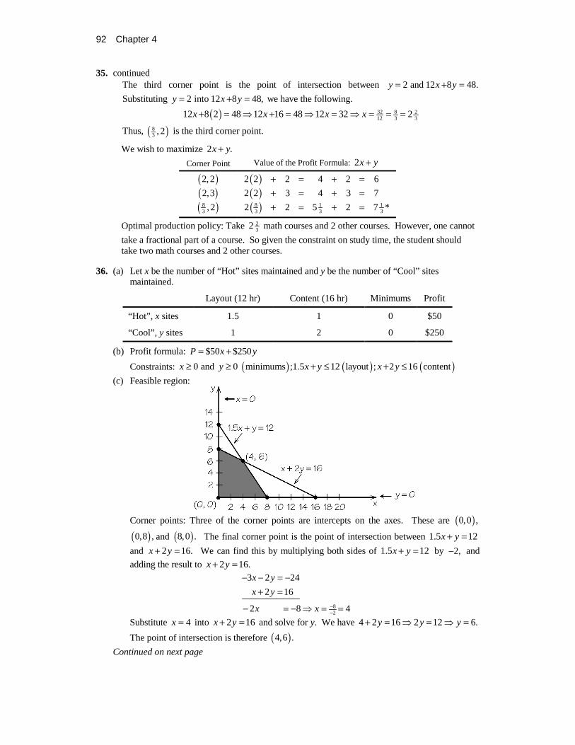
36. (a) Let x be the number of “Hot” sites maintained and y be the number of “Cool” sites maintained.

Layout (12 hr) Content (16 hr) Minimums Profit

“Hot”, x sites 1.5 1 0 $50

“Cool”, y sites 1 2 0 $250


Constraints: ( ) ( ) ( )0 and 0 minimums ;1.5 12 layout ; 2 16 contentx y x y x y≥ ≥ + ≤ + ≤


Corner points: Three of the corner points are intercepts on the axes. These are ( )0,0 ,

( )0,8 , and ( )8,0 . The final corner point is the point of intersection between 1.5 12x y+ =

and 2 16.x y+ = We can find this by multiplying both sides of 1.5 12x y+ = by 2,− and

adding the result to 2 16.x y+ =

82

3 2 24

2 16

2 8 4

x y

x y

x x −−

− − = −+ =

− = − ⇒ = =

Substitute 4x = into 2 16x y+ = and solve for y. We have 4 2 16 2 12 6.y y y+ = ⇒ = ⇒ =




36. continued



( )( )( )( )

0,0

0,8

8,0

4,6

( ) ( )( ) ( )( )( )

( )( )

$50 0 $250 0 $0 $0 $0

$50 0 $250 8 $0 $2000 $2000*

$50 8 $250 0 $400 $0 $400

$200 $1500 $1700$50 4 $250 6

+ = + =+ = + =

+ = + =+ = + =

Optimal production policy: Maintain no “hot” and 8 “cool” sites.

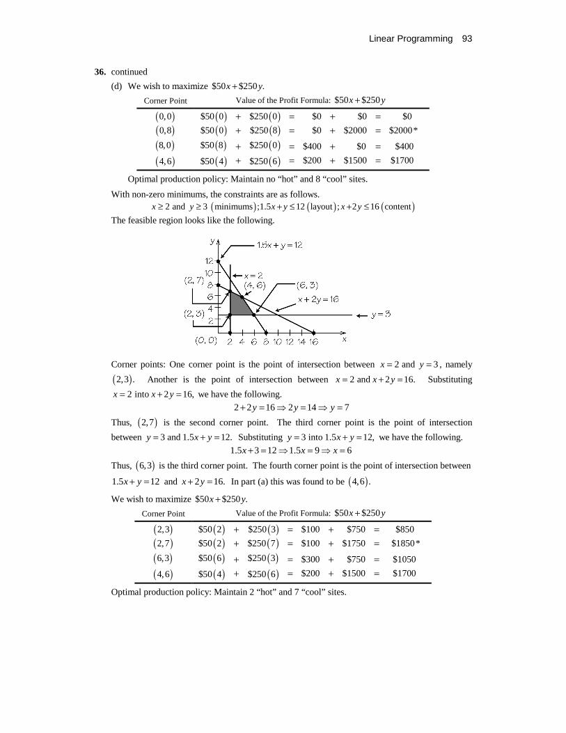
With non-zero minimums, the constraints are as follows. ( ) ( ) ( )2 and 3 minimums ;1.5 12 layout ; 2 16 contentx y x y x y≥ ≥ + ≤ + ≤



( )2,3 . Another is the point of intersection between 2 and 2 16.x x y= + = Substituting

2 into 2 16,x x y= + = we have the following.

2 2 16 2 14 7y y y+ = ⇒ = ⇒ =


between 3 and 1.5 12.y x y= + = Substituting 3 into 1.5 12,y x y= + = we have the following.

1.5 3 12 1.5 9 6x x x+ = ⇒ = ⇒ =

Thus, ( )6,3 is the third corner point. The fourth corner point is the point of intersection between

1.5 12x y+ = and 2 16.x y+ = In part (a) this was found to be ( )4,6 .



( )( )( )( )

2,3

2,7

6,3

4,6

( ) ( )( ) ( )( )( )

( )( )

$50 2 $250 3 $100 $750 $850

$50 2 $250 7 $100 $1750 $1850*

$50 6 $250 3 $300 $750 $1050

$200 $1500 $1700$50 4 $250 6

+ = + =+ = + =

+ = + =+ = + =

Optimal production policy: Maintain 2 “hot” and 7 “cool” sites.

94 Chapter 4

37. (a) Let x be the number of Grade A batches and y be the number of Grade B batches.

Scrap cloth

(100 lb) Scrap Paper

(120 lb) Minimums Profit

Grade A, x batches 25 10 0 $500

Grade B, y batches 10 20 0 $250


Constraints: ( ) ( ) ( )0 and 0 minimums ;25 10 100 cloth ;10 20 120 paperx y x y x y≥ ≥ + ≤ + ≤



( )0,6 , and ( )4,0 . The final corner point is the point of intersection between

25 10 100x y+ = and 10 20 120.x y+ = We can find this by multiplying both sides of

25 10 100x y+ = by 2,− and adding the result to 10 20 120.x y+ =

8040

50 20 200

10 20 120

40 80 2

x y

x y

x x −−

− − = −+ =

− = − ⇒ = =

Substitute 2x = into 25 10 100x y+ = and solve for y. We have the following.

( )25 2 10 100 50 10 100 10 50 5y y y y+ = ⇒ + = ⇒ = ⇒ =




( )( )( )( )

0,0

0,6

4,0

2,5

( ) ( )( ) ( )( )( )

( )( )

$500 0 $250 0 $0 $0 $0

$500 0 $250 6 $0 $1500 $1500

$500 4 $250 0 $2000 $0 $2000

$1000 $1250 $2250*$500 2 $250 5

+ = + =+ = + =

+ = + =+ = + =

Optimal production policy: Make 2 grade A and 5 grade B batches.

With non-zero minimums 1x ≥ and 1,y ≥ there will be no change because the optimal

production policy already obeys these non-zero minimums.


38. (a) Let x be the number of modest houses and y be the number of deluxe houses.

Space

(100 acres) Money in thousands

($2600) Minimums

Profit in thousands

Modest, x houses 1 $20 0 $25

Deluxe, y houses 1 $40 0 $60


Constraints: ( )( )

( )

0 and 0 minimums

100 space

20 40 2600 available funds

x y

x y

x y

≥ ≥

+ ≤

+ ≤



( )0,65 , and ( )130,0 . The final corner point is the point of intersection between 100x y+ =

and 20 40 2600.x y+ = We can find this by multiplying both sides of 100x y+ = by 20,−

and add the result to 20 40 2600.x y+ =

20 20 2000

20 40 2600

20 600 30

x y

x y

y y

− − = −+ =

= ⇒ =

Substitute 30y = into 100x y+ = and solve for y. We have 30 100 70.x x+ = ⇒ = The

point of intersection is therefore ( )70,30 .


Corner Point Value of the Profit Formula: $25 $60x y+ (in thousands)

( )( )

( )( )

0,0

0,65

100,0

70,30

( ) ( )( ) ( )

( )( )

( )( )

$25 0 $60 0 $0 $0 $0

$25 0 $60 65 $0 $3900 $3900*

$25 100 $60 0 $2500 $0 $2500

$1750 $1800 $3550$25 70 $60 30

+ = + =+ = + =

+ = + =+ = + =

Optimal production policy: Build no modest and 65 deluxe houses. Continued on next page

96 Chapter 4

38. continued

With non-zero minimums, the constraints are as follows. ( ) ( ) ( )20 and 20 minimums ; 100 space ;20 40 2600 available fundsx y x y x y≥ ≥ + ≤ + ≤


Corner points: One corner point is the point of intersection between 20 and 20,x y= = namely

( )20, 20 . Another is the point of intersection between 20 and 100.y x y= + = Substituting

20 into 100,y x y= + = we have 20 100 80.x x+ = ⇒ = Thus, ( )80, 20 is the second corner

point. The third corner point is the point of intersection between 20 and 20 40 2600.x x y= + =


( )20 20 40 2600 400 40 2600 40 2200 55y y y y+ = ⇒ + = ⇒ = ⇒ =

Thus, ( )20,55 is the third corner point. The fourth corner point is the point of intersection

between 100x y+ = and 20 40 2600.x y+ = In part (a) this was found to be ( )70,30 .


Corner Point Value of the Profit Formula: $25 $60x y+ (in thousands)

( )( )( )( )

20, 20

20,55

80, 20

70,30

( ) ( )( ) ( )( )( )

( )( )

$25 20 $60 20 $500 $1200 $1700

$25 20 $60 55 $500 $3300 $3800*

$25 80 $60 20 $2000 $1200 $3200

$1750 $1800 $3550$25 70 $60 30

+ = + =+ = + =

+ = + =+ = + =

Optimal production policy: Make 20 modest and 55 deluxe houses.


39. (a) Let x be the number of cartons of regular soda and y be the number of cartons of diet soda.

Cartons (5000) Money ($5400) Minimums Profit

Regular, x cartons 1 $1.00 600 $0.10

Diet, y cartons 1 $1.20 1000 $0.11

(b) Profit formula: $0.10 $0.11P x y= +

Constraints: ( )( ) ( )

600 and 1000 minimums

5000 cartons ;1.00 1.20 5400 money

x y

x y x y

≥ ≥

+ ≤ + ≤



namely ( )600,1000 . Another is the point of intersection between

1000 and 5000.y x y= + = Substituting 1000 into 5000,y x y= + = we have

1000 5000 4000.x x+ = ⇒ = Thus, ( )4000,1000 is the second corner point. The third

corner point is the point of intersection between 600 and 1.00 1.20 5400.x x y= + =

Substituting 600 into 1.00 1.20 5400,x x y= + = we have the following.

( )1.00 600 1.20 5400 600 1.20 5400 1.20 4800 4000y y y y+ = ⇒ + = ⇒ = ⇒ =

Thus, ( )600,4000 is the third corner point. The fourth corner point is the point of

intersection between 5000x y+ = and 1.00 1.20 5400.x y+ = We can find this by

multiplying both sides of 5000x y+ = by 1,− and adding the result to 1.00 1.20 5400.x y+ =

5000

1.00 1.20 5400

0.20 400 2000

x y

x y

y y

− − = −+ =

= ⇒ =

Substitute 2000y = into 5000x y+ = and solve for y. We have 2000 5000x + = or

3000.x = The point of intersection is therefore ( )3000,2000 .

(d) We wish to maximize $0.10 $0.11 .x y+


( )( )( )

( )

600,1000

4000,1000

600, 4000

3000,2000

( ) ( )( ) ( )( )( )

( )( )

$0.10 600 $0.11 1000 $60 $110 $170

$0.10 4000 $0.11 1000 $400 $110 $510

$0.10 600 $0.11 4000 $60 $440 $500

$300 $220 $520*$0.10 3000 $0.11 2000

+ = + =+ = + =

+ = + =+ = + =

Optimal production policy: Make 3000 cartons of regular and 2000 cartons of diet.

With zero minimums there is no change in the optimal production policy because the corresponding corner point does not touch either line from a minimum constraint.

98 Chapter 4

40. (a) Let x be the number of pheasants and y be the number of partridges.

Bird count (100) Cost ($2400) Minimums Profit

Pheasants, x 1 $20 0 $14

Partridges, y 1 $30 0 $16


Constraints: ( ) ( ) ( )0 and 0 minimums ; 100 bird count ;20 30 2400 moneyx y x y x y≥ ≥ + ≤ + ≤



( )0,80 , and ( )100,0 . The final corner point is the point of intersection between 100x y+ =

and 20 30 2400.x y+ = We can find this by multiplying both sides of 100x y+ = by 20,−

and adding the result to 20 30 2400.x y+ =

20 20 2000

20 30 2400

10 400 40

x y

x y

y y

− − = −+ =

= ⇒ =

Substitute 40y = into 100x y+ = and solve for y. We have 40 100 60.x x+ = ⇒ = The

point of intersection is therefore ( )60,40 .



( )( )( )( )

0,0

0,80

100,0

60,40

( ) ( )( ) ( )

( )( )

( )( )

$14 0 $16 0 $0 $0 $0

$14 0 $16 80 $0 $1280 $1280

$14 100 $16 0 $1400 $0 $1400

$840 $640 $1480*$14 60 $16 40

+ = + =+ = + =

+ = + =+ = + =

Optimal production policy: Raise 60 pheasants and 40 partridges.

With nonzero minimum of 20x ≥ and 10,y ≥ there is no change because the optimal

production policy obeys these minimums.


41. (a) Let x be the number of desk lamps and y be the number of floor lamps.

Labor (1200 hr) Money ($4200) Minimums Profit

Desk, x lamps 0.8 $4 0 $2.65

Floor, y lamps 1.0 $3 0 $4.67


Constraints: ( )( )

( )

0 and 0 minimums

0.8 1.0 1200 labor

4 3 4200 money

x y

x y

x y

≥ ≥

+ ≤

+ ≤




0.8 1.0 1200x y+ = and 4 3 4200.x y+ = We can find this by multiplying both sides of

0.8 1.0 1200x y+ = by 3,− and adding the result to 4 3 4200.x y+ =

2.4 3 3600

4 3 4200

1.6 600 375

x y

x y

x x

− − = −+ =

= ⇒ =

Substitute 375x = into 0.8 1.0 1200x y+ = and solve for y. We have the following.

( )0.8 375 1200 300 1200 900y y y+ = ⇒ + = ⇒ =




( )( )( )

( )

0,0

0,1200

1050,0

375,900

( ) ( )( ) ( )

( )( )

( )( )

$2.65 0 $4.67 0 $0.00 $0.00 $0.00

$2.65 0 $4.67 1200 $0.00 $5604.00 $5604.00*

$2.65 1050 $4.67 0 $2782.50 $0.00 $2782.50

$993.75 $4203.00 $5196.75$2.65 375 $4.67 900

+ = + =+ = + =

+ = + =+ = + =

Optimal production policy: Make no desk lamps and 1200 floor lamps. Continued on next page

100 Chapter 4

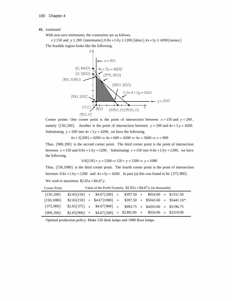
41. continued

With non-zero minimums, the constraints are as follows.

( ) ( ) ( )150 and 200 minimums ;0.8 1.0 1200 labor ;4 3 4200 moneyx y x y x y≥ ≥ + ≤ + ≤



namely ( )150,200 . Another is the point of intersection between 200 and 4 3 4200.y x y= + =

Substituting 200 into 4 3 4200,y x y= + = we have the following.

( )4 3 200 4200 4 600 4200 4 3600 900x x x x+ = ⇒ + = ⇒ = ⇒ =

Thus, ( )900, 200 is the second corner point. The third corner point is the point of intersection

between 150 and 0.8 1.0 1200.x x y= + = Substituting 150 into 0.8 1.0 1200 ,x x y= + = we have

the following.

( )0.8 150 1200 120 1200 1080y y y+ = ⇒ + = ⇒ =

Thus, ( )150,1080 is the third corner point. The fourth corner point is the point of intersection

between 0.8 1.0 1200x y+ = and 4 3 4200.x y+ = In part (a) this was found to be ( )375,900 .

We wish to maximize $2.65 $4.67 .x y+

Corner Point Value of the Profit Formula: $2.65 $4.67x y+ (in thousands)

( )( )( )( )

150,200

150,1080

375,900

900, 200

( ) ( )( ) ( )( )( )

( )( )

$2.65 150 $4.67 200 $397.50 $934.00 $1331.50

$2.65 150 $4.67 1080 $397.50 $5043.60 $5441.10*

$2.65 375 $4.67 900 $993.75 $4203.00 $5196.75

$2385.00 $934.00 $3319.00$2.65 900 $4.67 200

+ = + =+ = + =

+ = + =+ = + =

Optimal production policy: Make 150 desk lamps and 1080 floor lamps.


For Exercises 42 – 45, part (c) (using a simplex algorithm program) will not be addressed in the solutions.

42. (a) Let x be the number of toy A, y be the number of toy B, and z be the number of toy C.

Shaper (50) Smoother (40) Painter (60) Minimums Profit

Toy A, x 1 2 1 0 $4

Toy B, y 2 1 3 0 $5

Toy C, z 3 2 1 0 $9

(b) Profit formula: $4 $5 $9P x y z= + +

Constraints: ( )( )( )

( )

0, 0, and 0 minimums

2 3 50 shaper

2 2 40 smoother

3 60 painter

x y z

x y z

x y z

x y z

≥ ≥ ≥

+ + ≤

+ + ≤

+ + ≤

(c) Optimal product policy: Make 5 toy A, no toy B, 15 toy C for a profit of $155.

43. (a) Let x be the number of chairs, y be the number of tables, and z be the number of beds.

Chis (80 hr) Sue (200 hr) Juan (200) Minimums Profit

Chairs, x 1 3 2 0 $100

Tables, y 3 5 4 0 $250

Beds, z 5 4 8 0 $350


Constraints: ( )( ) ( ) ( )


3 5 80 Chris ;3 5 4 200 Sue ;2 4 8 200 Juan

x y z

x y z x y z x y z

≥ ≥ ≥

+ + ≤ + + ≤ + + ≤

(c) Optimal product policy: Make 50 chairs, 10 tables, and no beds each month for a profit of 7500 in one month.

44. (a) Let x be the number of boxes of Special Mix, y be the number of boxes of Regular Mix, and z be the number of boxes of Purist Mix.

Chocolate (1000 lb)

Nuts (200 lb)

Fruit (100 lb)

Minimums Profit

Special, x boxes 3 1 1 0 $10

Regular, y boxes 4 0.5 0 0 $6

Purist, z boxes 5 0 0 0 $4



( )


3 4 5 1000 chocolate

0.5 0 200 nuts

0 0 100 fruit

x y z

x y z

x y z

x y z

≥ ≥ ≥

+ + ≤

+ + ≤

+ + ≤

(c) Optimal product policy: Make 100 boxes of Special, 175 boxes of Regular, and 0 boxes of Purist for a profit of $2050.

102 Chapter 4

45. (a) Let w be the number of pounds of Excellent coffee, x be the number of pounds of Southern coffee, y be the number of pounds of World coffee, and z be the number of pounds of Special coffee.

African (17,600 oz)

Brazilian (21,120 oz)

Columbian (12,320 oz)

Minimums Profit

Excellent, w pounds 0 0 16 0 $1.80

Southern, x pounds 0 12 4 0 $1.40

World, y pounds 6 8 2 0 $1.20

Special, z pounds 10 6 0 0 $1.00

(b) Profit formula: $1.80 $1.40 $1.20 $1.00P w x y z= + + +

Constraints: ( )( )

( )( )

0, 0, 0, and 0 minimums

0 0 6 10 17,600 African

0 12 8 6 12,120 Brazilian

16 4 2 6 12,320 Columbian

w x y z

w x y z

w x y z

w x y z

≥ ≥ ≥ ≥

+ + + ≤

+ + + ≤

+ + + ≤

(c) Optimal product policy: Make 470 pounds of Excellent, none of Southern, 2400 pounds of World, and 320 pounds for a profit of $4046.

46. Minimize 4 7C x y= + subject to 3; 2; 10;2 3 24x y x y x y≥ ≥ + ≤ + ≤

The corner points are ( ) ( ) ( ) ( )3,6 , 3,2 , 8, 2 , and 6, 4 .

We wish to minimize 4 7 .C x y= +

Corner Point

Value of the cost: 4 7x y+

( )( )( )( )

3,6

3,2

8,2

6,4

( ) ( )( ) ( )( )( )

( )( )

4 3 7 6 12 42 54

4 3 7 2 12 14 26*

4 8 7 2 32 14 46

24 28 524 6 7 4

+ = + =+ = + =

+ = + =+ = + =

The minimum value occurs at the corner point ( )3,2 , where C is equal to 26.


47. Minimize 3 11C x y= + subject to 2; 3; 3 18;6 4 48x y x y x y≥ ≥ + ≤ + ≤

The corner points are ( ) ( ) ( ) ( )2,3 , 5,3 , 4,6 , and 2,9 .

We wish to minimize 3 11 .C x y= +

Corner Point

Value of the Profit Formula: 3 11x y+

( )( )( )( )

2,3

5,3

4,6

2,9

( ) ( )( ) ( )( )( )

( )( )

3 2 11 3 6 33 39*

3 5 11 3 15 33 48

3 4 11 6 12 66 78

6 99 1053 2 11 9

+ = + =+ = + =

+ = + =+ = + =

The minimum value occurs at the corner point ( )2,3 , where C is equal to 39.

48. The only feasible point with integer coordinates for the collection of inequalities 0, 0x y≥ ≥

and 0.5x y+ = is ( )0,0 .

49. (a) Let x be the number of business calls and y be the charity calls.

Time (240 min) Minimums Profit

Business, x calls 4 0 $0.50 Charity, y calls 6 0 $0.40





( )60,0 .


104 Chapter 4

49. continued


Corner Point

Value of the Profit Formula: $0.50 $0.40x y+

( )( )( )

0,0

0,40

60,0

( ) ( )( ) ( )

( ) ( )

$0.50 0 $0.40 0 $0.00 $0.00 $0.00

$0.50 0 $0.40 40 $0.00 $16.00 $16.00

$0.50 60 $0.40 0 $30.00 $0.00 $30.00*

+ = + =+ = + =+ = + =

Optimal production policy: Make 60 business and no charity calls. With non-zero minimums, the constraints are as follows.

( ) ( )12 and 10 minimums ;4 6 240 timex y x y≥ ≥ + ≤





( )4 12 6 240 48 6 240 6 192 32y y y y+ = ⇒ + = ⇒ = ⇒ =


between 10 and 4 6 240.y x y= + = Substituting 10 into 4 6 240y x y= + = we have the

following.

( )4 6 10 240 4 60 240 4 180 45x x x x+ = ⇒ + = ⇒ = ⇒ =


We wish to maximize $0.50 $0.40 .x y+

Corner Point


( )( )( )

12,10

12,32

45,10

( ) ( )( ) ( )( ) ( )

$0.50 12 $0.40 10 $6.00 $4.00 $10.00

$0.50 12 $0.40 32 $6.00 $12.80 $18.80

$0.50 45 $0.40 10 $22.50 $4.00 $26.50*

+ = + =+ = + =+ = + =

Optimal production policy: Make 45 business and 10 charity calls.


50. (a) Let x be the number of gallons of premium and y be the number of gallons of regular.

High Octane

(500 gal.)

Low Octane

(600 gal.) Minimums Profit

Premium, x gallons 0.5 0.5 0 $0.40

Regular, y gallons 0.25 0.75 0 $0.30



0 and 0 minimums

0.5 0.25 500 high octane

0.5 0.75 600 low octane

x y

x y

x y

≥ ≥

+ ≤

+ ≤




0.5 0.25 500x y+ = and 0.5 0.75 600.x y+ = We can find this by multiplying both sides of

0.5 0.25 500x y+ = by 1,− and adding the result to 0.5 0.75 600.x y+ =

0.5 0.25 500

0.5 0.75 600

0.50 100 200

x y

x y

y y

− − = −+ =

= ⇒ =

Substitute 200y = into 0.5 0.25 500x y+ = and solve for x. We have the following.

( )0.5 0.25 200 500 0.5 50 500 0.5 450 900x x x x+ = ⇒ + = ⇒ = ⇒ =



Corner Point


( )( )

( )( )

0,0

0,800

1000,0

900,200

( ) ( )( ) ( )

( )( )

( )( )

$0.40 0 $0.30 0 $0 $0 $0

$0.40 0 $0.30 800 $0 $240 $240

$0.40 1000 $0.30 0 $400 $0 $400

$360 $60 $420*$0.40 900 $0.30 200

+ = + =+ = + =

+ = + =+ = + =

Optimal production policy: Make 900 gallons of premium and 200 gallons of regular.



106 Chapter 4

51. (a) Let x be the number of bikes and y be the number of wagons.

Machine (12 hr) Paint(16 hr.) Minimums Profit

Bikes, x 2 4 0 $12

Wagons, y 3 2 0 $10


Constraints: ( ) ( ) ( )0 and 0 minimums ;2 3 12 machine ;4 2 16 paintx y x y x y≥ ≥ + ≤ + ≤



( )0,4 , and ( )4,0 . The final corner point is the point of intersection between 2 3 12x y+ =

and 4 2 16.x y+ = We can find this by multiplying both sides of 2 3 12x y+ = by 2,− and

adding the result to 4 2 16.x y+ =

4 6 24

4 2 16

4 8 2

x y

x y

y y

− − = −+ =

− = − ⇒ =

Substitute 2y = into 4 2 16x y+ = and solve for x. We have the following.

( )4 2 2 16 4 4 16 4 12 3x x x x+ = ⇒ + = ⇒ = ⇒ =



Corner Point

Value of the Profit Formula: $12 $10x y+

( )( )( )( )

0,0

0,4

4,0

3,2

( ) ( )( ) ( )( )( )

( )( )

$12 0 $10 0 $0 $0 $0

$12 0 $10 4 $0 $40 $40

$12 4 $10 0 $48 $0 $48

$36 $20 $56*$12 3 $10 2

+ = + =+ = + =

+ = + =+ = + =

Optimal production policy: Make 3 bikes and 2 wagons.




52. (a)

(b)


108 Chapter 4

52. continued

(c)

(d) Answers will vary.

For (a) we might have two companies that supply a total of 11 units of lemon ices, and two stores that require 11 units of lemon ices. For (b) we have two coal mines which can supply a total of 9 units of coal, and three coal burning power plants which require 9 units of coal. For (c) we have three orchards which can supply 10 units of apples and two supermarket chains which require 10 units of apples.

(e) For (a) the cost is ( ) ( ) ( )2 3 6 5 3 2 6 30 6 42.+ + = + + =

For (b) the cost is ( ) ( ) ( ) ( )1 11 1 6 2 9 5 2 11 6 18 10 45.+ + + = + + + =

For (c) the cost is ( ) ( ) ( ) ( )1 17 1 1 4 9 4 6 17 1 36 24 78.+ + + = + + + =


53. (a)

(b) The cost for this solution is ( ) ( ) ( ) ( )1 1 1 3 2 4 1 5 1 3 8 5 17.+ + + = + + + =

(c) The indicator value for cell ( )I, 2 is 7 1 3 4 5.− + − =

The indicator value for cell ( )I,3 is 2 1 3 5 1.− + − = −

110 Chapter 4

54. (a)

(b) The indicator value for cell ( )II,1 is 3 13 1 4 13.− + − = −

The indicator value for cell ( )I,3 is 2 1 4 1 4.− + − =



54. continued

(c) The cost for this solution is ( ) ( ) ( ) ( )1 13 1 1 2 4 1 1 13 1 8 1 23.+ + + = + + + =

We get a cheaper solution, as shown below, by shipping using cell ( )II,1 .

The new solution has cost ( ) ( ) ( ) ( )2 1 1 3 1 4 1 1 2 3 4 1 10.+ + + = + + + = This saves 13 units of

cost over the previous solution, as would be expected because the indicator value is 13,−

and we shipped one more unit via cell ( )II,1 .

55. (a) The graph is a tree because it is connected and has no circuit.

(b) If we add the edge joining Vertex I to Vertex 2 we get the circuit 2, I, 1, II, 2.

If we add the edge from Vertex I to Vertex 3 we get the circuit 3, I, 1, II, 3.

(c) For the circuit 2, I, 1, II, 2 it corresponds to the following circuit of cells.

( ) ( ) ( ) ( ) ( )I,2 , I,1 , II,1 , II,2 , I,2

For the circuit 3, I, 1, II, 3 it corresponds to the following circuit of cells.

( ) ( ) ( ) ( ) ( )I,3 , I,1 , II,1 , II,3 , I,3

112 Chapter 4

56. (a)

In row I the minimum cost is 1 ( )( )cell I, 2 and for row II the minimum cost is 2

( )( )cell II,1 . Thus, the row with the minimum value is row 1. Since this minimum cost

occurs in column 2, we try shipping as much as we can via this cell. This means we can ship 2 units in ( )cell I, 2 . So we cross out column 2, and reduce the rim condition for row I

to a 1. We now have a 2 2× tableau. We find the minimum cost for row I is 3 (there is a tie for two different cells) and the minimum cost for row II is 2, in ( )cell II,1 . So the row with minimum value is row II; so in

this row we ship as much as we can via cell (II,1). We can ship 4 via this cell, so now we cross out column 1. The rim value for this row is reduced from 5 to 1. We now have a tableau with one column (column 3) and two rows; row I has a minimum of 3 and row II a minimum of 4; so we ship first via the minimum row cost (row I whose cost is 3) in

( )cell I,3 (1 unit) and cross out row I, and finally, in ( )cell II,3 , 1 unit (cost 4).

So the cells with circled numbers are: ( )I, 2 with a 2; ( )I,3 with a 1; ( )II,1 with a 4; and

( )II,3 with a 1.

(b) The cost of the solution above is ( ) ( ) ( ) ( )2 1 1 3 4 2 1 4 2 3 8 4 17.+ + + = + + + =



56. continued

(c)

The cost of this solution is ( ) ( ) ( ) ( )3 13 1 2 2 5 2 4 39 2 10 8 59,+ + + = + + + = which is 42 units

more expensive than the solution we found in (b). It is often worth using a more complex method to find a better initial solution to a problem than using a simple method, which finds a poor initial solution, as the Northwest Corner Rule does for this problem.

114 Chapter 4

57. (a) (i)

(ii) Since the rim values are the same, the end result will be the same (relative to the new table)



57. (a) continued

(iii)

(b) For (i) the indicator value for each non-circled cell is calculated as follows.

( )cell II,1 : 4 6 3 1 0− + − =

( )cell II, 2 : 5 6 3 2 0− + − =

The tableau shown is optimal. However, there are also other optimal tableaux, as can be seen from the fact that the indicator values for each of the cells that have no circled entries are 0.


116 Chapter 4

57. (b) continued

For (ii) the indicator value for each non-circled cell is calculated as follows.

( )cell II,1 : 3 1 4 6 0− + − =

( )cell II, 2 : 2 1 4 5 0− + − =

The tableau shown is optimal, although there are also other optimal tableaux.

For (iii) the indicator value for each non-circled cell is calculated as follows.

( )cell II,1 : 2 4 1 6 3− + − = −

( )cell II, 2 : 3 4 1 5 5− + − = −

The tableau shown is not optimal. The current cost is as follows.

( ) ( ) ( ) ( )2 6 1 5 2 1 4 4 12 5 2 16 35+ + + = + + + =



57. (b) continued

Since ( )cell II,1 has a more negative indicator value, we can reduce the cost more by

using that cell. Increasing by 2, we obtain the following tableau.

The cost is now ( ) ( ) ( ) ( )1 5 4 1 2 4 2 2 5 4 8 4 21.+ + + = + + + = We can reduce the cost more

by using ( )cell II, 2 . Increasing by 1, we obtain the following tableau.

The cost is now ( ) ( ) ( ) ( )2 2 1 3 1 4 5 1 4 3 4 5 16.+ + + = + + + =

118 Chapter 4

58. (a)

(b) The cost is given by ( ) ( ) ( ) ( ) ( )1 3 2 1 1 6 5 3 1 5 3 2 6 15 5 31.+ + + + = + + + + =



58. continued (c) The indicator value for ( )cell II,1 is 5 3 6 3 5.− + − =

The indicator value for ( )cell II, 2 is 2 3 6 1 4.− + − =

The indicator value for ( )cell III,1 is 1 5 6 3 1.− + − = −


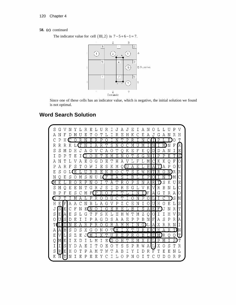
120 Chapter 4

58. (c) continued

The indicator value for ( )cell III, 2 is 7 5 6 1 7.− + − =

Since one of these cells has an indicator value, which is negative, the initial solution we found is not optimal.

Word Search Solution

Documents

FAPP07 ism 04 - University of Wisconsin–Madison