Embed Size (px)
Citation preview

Lecture 2.2 Social and Resource Accounting:
Multiplier Analysis
David Roland-Holst, Sam Heft-Neal, and Anaspree Chaiwan UC Berkeley and Chiang Mai University
Training Workshop Economywide Assessment of High Impact Animal Disease
14-18 January 2013 InterContinental Hotel, Phnom Penh, Cambodia
Roland-Holst 2 15 January 2013
SAM Multipliers
• SAM multipliers are similar to I/O multipliers in both their algebra and economic interpretation.
• However, where the I/O multipliers are “open,” SAM multipliers reflect closed circular flow of income effects, so we can look at both: – Induced effects through income-expenditure linkages – Distribution of income through institutional accounts
• The general idea with most SAM multiplier analyses is to examine two groups of actors (producers and households) interacting in two markets (commodity and factor).
Roland-Holst 3 15 January 2013
Endogenous and Exogenous Accounts
• To calculate SAM multipliers we need to first separate the SAM into endogenous and exogenous accounts, both for economic and mathematical reasons.
• Economically, the SAM does not describe all of the factors at work in an economy (e.g., government spending habits).
• Mathematically, without exogenizing some accounts we will end up with a singular A matrix and will not be able to calculate multipliers.
Roland-Holst 4 15 January 2013
Endogenous Accounts
• Endogenous accounts include those accounts where income-expenditure is governed by mechanisms that operate entirely within the SAM framework.
• Typically, endogenous accounts include: – Production-commodity accounts – Factor accounts – Household accounts – Capital account (sometimes)
Roland-Holst 5 15 January 2013
Exogenous Accounts
• Exogenous accounts are those accounts where income and/or expenditure are governed by forces external to the SAM framework.
• Typically, exogenous accounts include the government, ROW, and sometimes the capital account.
• For government and ROW, it should be fairly intuitive why these accounts are exogenous: The SAM tells us nothing about how government will plan expenditures, or what is happening in ROW.
Roland-Holst 6 15 January 2013
Endogenous and Exogenous Accounts
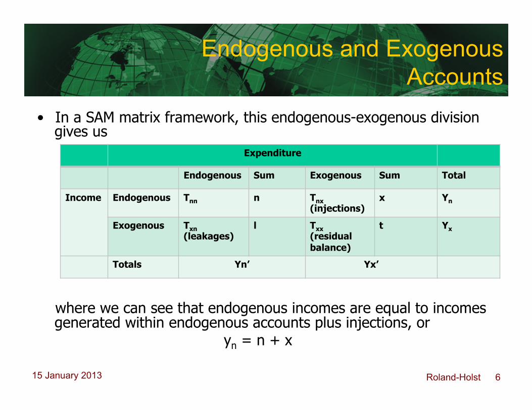
• In a SAM matrix framework, this endogenous-exogenous division gives us
where we can see that endogenous incomes are equal to incomes generated within endogenous accounts plus injections, or yn = n + x
Adapted from Khan, 2007
Expenditure
Endogenous Sum Exogenous Sum Total
Income Endogenous Tnn n Tnx (injections)
x Yn
Exogenous Txn (leakages)
l Txx (residual balance)
t Yx
Totals Yn’ Yx’
Roland-Holst 7 15 January 2013
Injections and Leakages
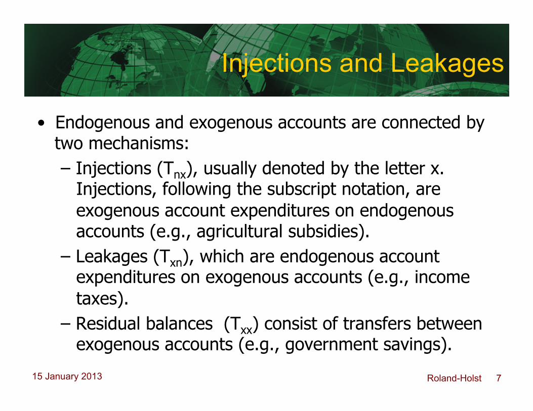
• Endogenous and exogenous accounts are connected by two mechanisms: – Injections (Tnx), usually denoted by the letter x.
Injections, following the subscript notation, are exogenous account expenditures on endogenous accounts (e.g., agricultural subsidies).
– Leakages (Txn), which are endogenous account expenditures on exogenous accounts (e.g., income taxes).
– Residual balances (Txx) consist of transfers between exogenous accounts (e.g., government savings).
Roland-Holst 8 15 January 2013
SAM A Matrix
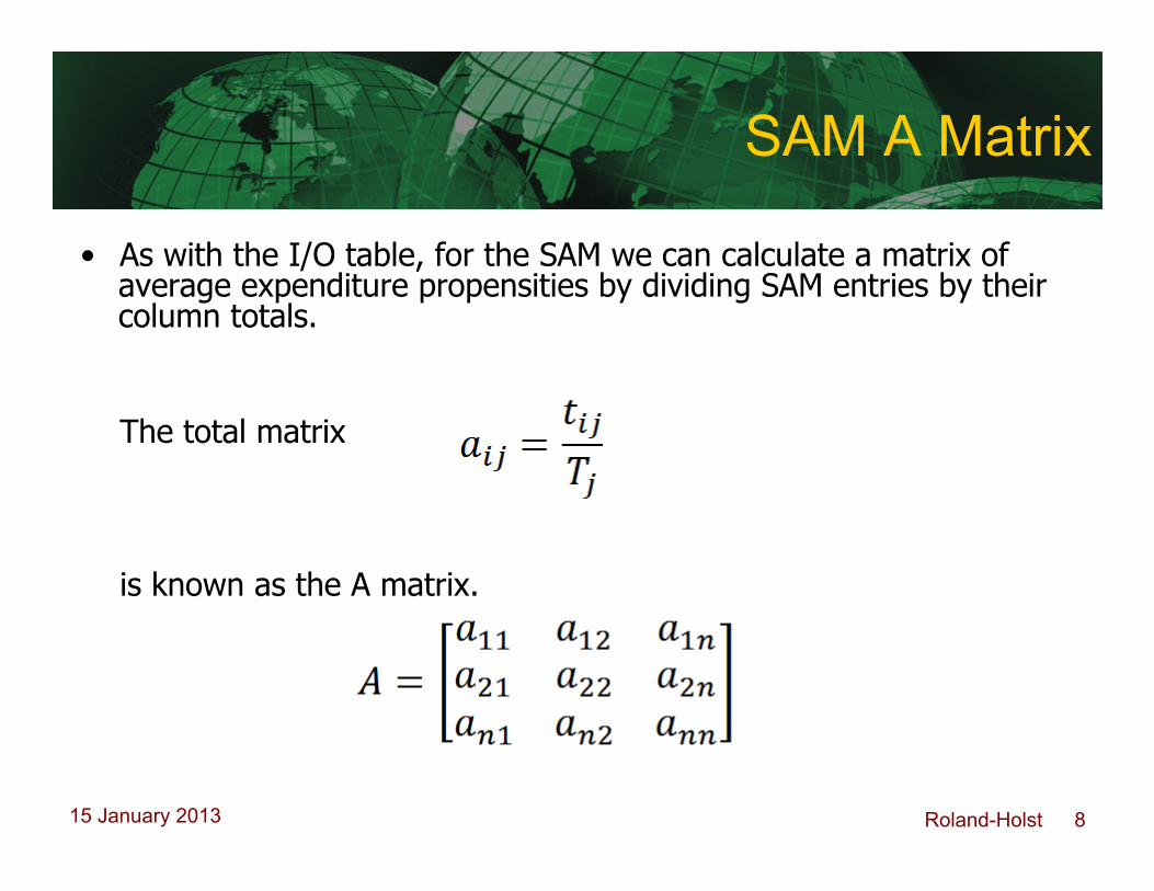
• As with the I/O table, for the SAM we can calculate a matrix of average expenditure propensities by dividing SAM entries by their column totals.
The total matrix
is known as the A matrix.
Roland-Holst 9 15 January 2013
SAM Multipliers
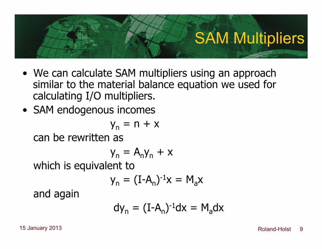
• We can calculate SAM multipliers using an approach similar to the material balance equation we used for calculating I/O multipliers.
• SAM endogenous incomes yn = n + x can be rewritten as yn = Anyn + x which is equivalent to yn = (I-An)-1x = Max and again dyn = (I-An)-1dx = Madx
Roland-Holst 10 15 January 2013
SAM Multipliers
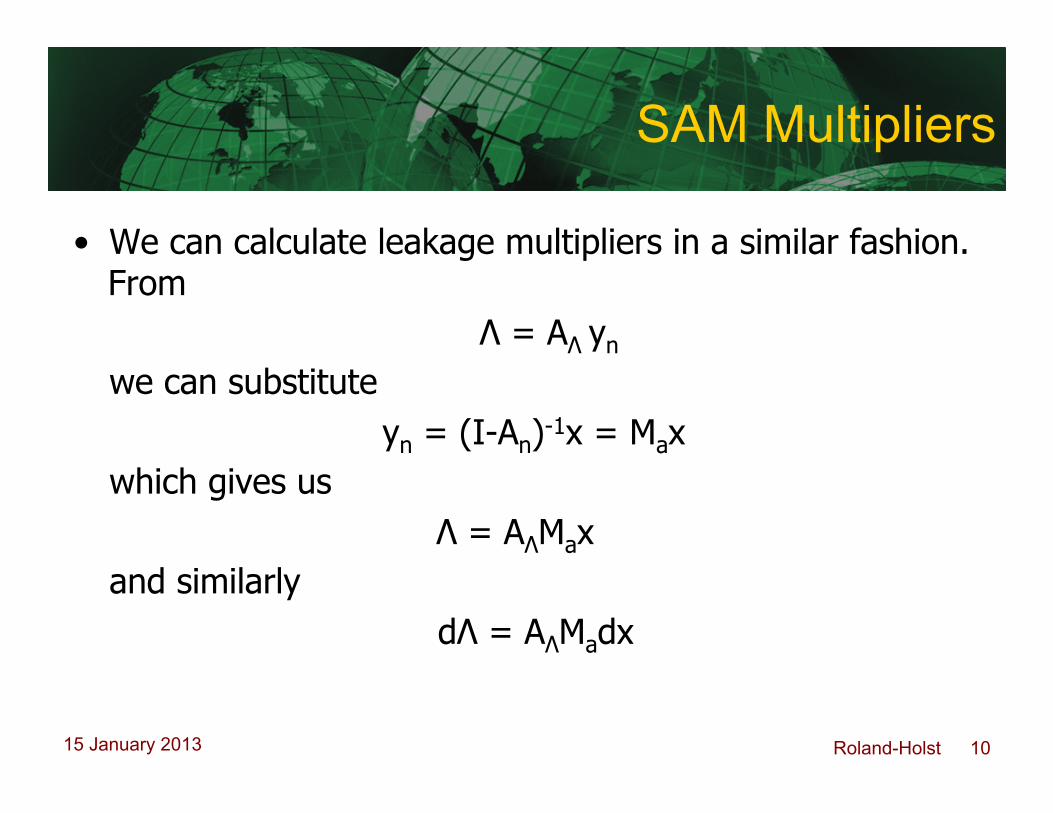
• We can calculate leakage multipliers in a similar fashion. From Λ = AΛ yn we can substitute yn = (I-An)-1x = Max which gives us Λ = AΛMax and similarly dΛ = AΛMadx
Roland-Holst 11 15 January 2013
SAM Multipliers
• As yn = Max suggests, the SAM multiplier Ma captures the multiplier effects of an exogenous shock x on endogenous income yn, where x is a vector of injections into endogenous (row) accounts.
Roland-Holst 12 15 January 2013
SAM Multiplier Limitations
• SAM multiplier limitations include: – Excess capacity in all sectors and unemployed or
underemployed factors of production; multipliers will overstate the total effects if capacity constraints exist.
– No allowance for substitution effects – Fixed prices – Limit to the endogenous effects that can be captured
(exogenous accounts will be affected by initial shock, leakage from endogenous to exogenous)

Roland-Holst 13 15 January 2013
Fixed-Price Multiplier Models
• While SAM multipliers can reveal interesting and policy-relevant information about economic structure and living standards, they do not contain information about economic behavior and are still accounting multipliers.
• Fixed-price multiplier (FPM) models add some behavioral characteristics into the SAM accounting framework by converting the SAM A matrix of average expenditure propensities into a matrix of marginal expenditure propensities.
Roland-Holst 14 15 January 2013
Partitioning the SAMn
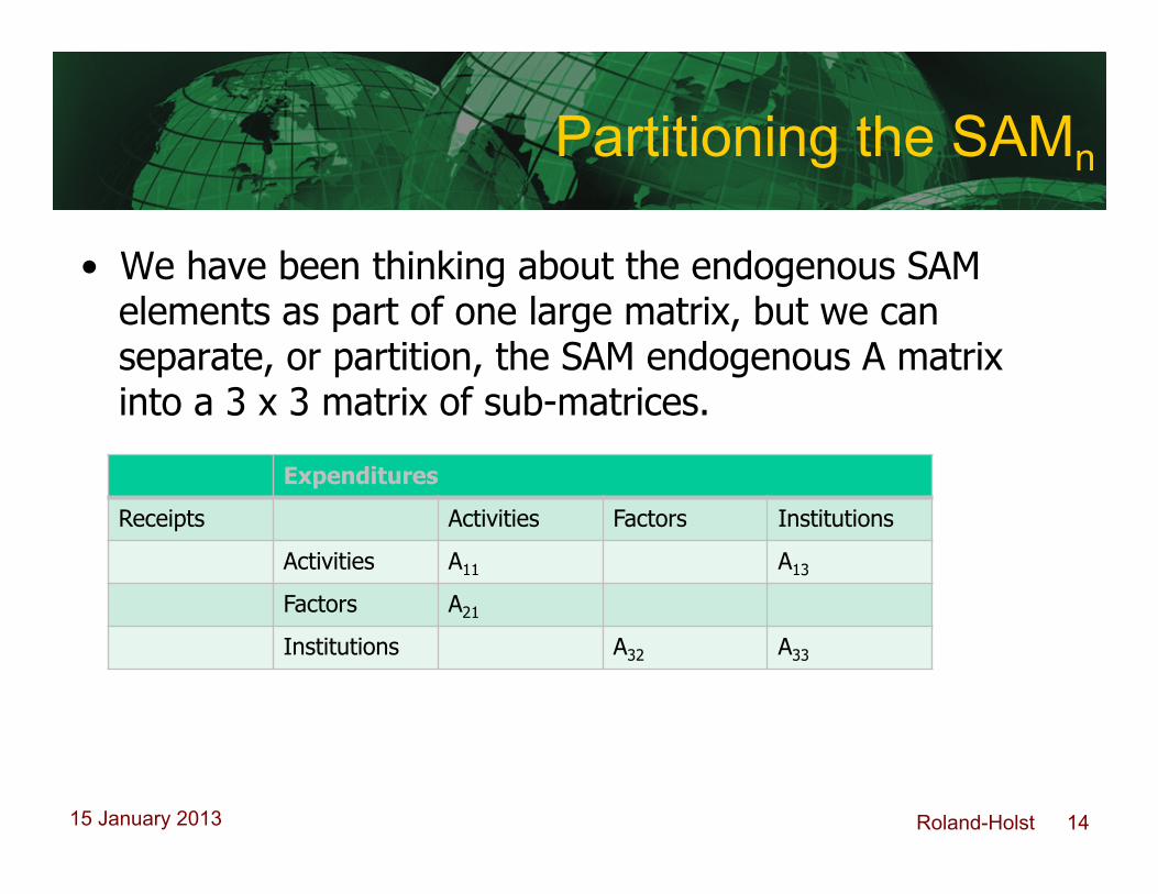
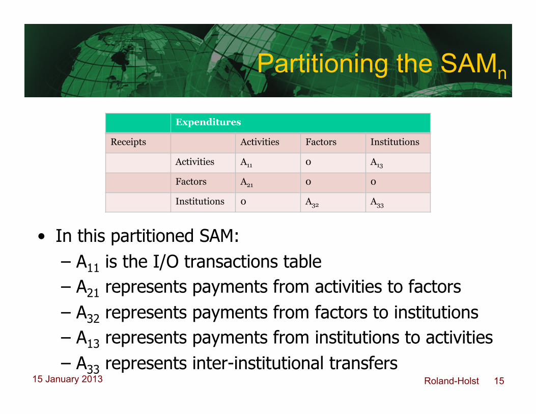
• We have been thinking about the endogenous SAM elements as part of one large matrix, but we can separate, or partition, the SAM endogenous A matrix into a 3 x 3 matrix of sub-matrices.
Expenditures
Receipts Activities Factors Institutions
Activities A11 A13
Factors A21
Institutions A32 A33
Roland-Holst 15 15 January 2013
Partitioning the SAMn
• In this partitioned SAM: – A11 is the I/O transactions table – A21 represents payments from activities to factors – A32 represents payments from factors to institutions – A13 represents payments from institutions to activities – A33 represents inter-institutional transfers
Expenditures
Receipts Activities Factors Institutions
Activities A11 0 A13
Factors A21 0 0
Institutions 0 A32 A33
Roland-Holst 16 15 January 2013
Partitioning the SAM
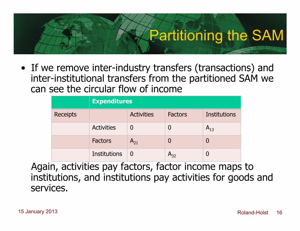
• If we remove inter-industry transfers (transactions) and inter-institutional transfers from the partitioned SAM we can see the circular flow of income
Again, activities pay factors, factor income maps to institutions, and institutions pay activities for goods and services.
Expenditures
Receipts Activities Factors Institutions
Activities 0 0 A13
Factors A21 0 0
Institutions 0 A32 0

Roland-Holst 17 15 January 2013
SAM Multiplier Decomposition
• Multiplier decomposition techniques allow us to separate multipliers into their component parts to examine different mechanisms within the economy.
• Multiplier components can be additive or multiplicative; in other words, multipliers can be the sum or the product of their component parts.
• We will begin with multiplicative SAM components, examine additive components, and finally demonstrate relationships among all three forms.
Roland-Holst 18 15 January 2013
Decomposition Algebra
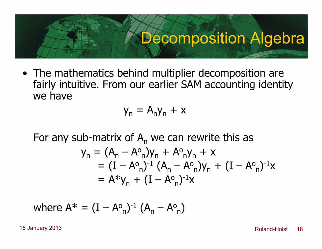
• The mathematics behind multiplier decomposition are fairly intuitive. From our earlier SAM accounting identity we have yn = Anyn + x
For any sub-matrix of An we can rewrite this as yn = (An – Ao
n)yn + Aonyn + x
= (I – Aon)-1 (An – Ao
n)yn + (I – Aon)-1x
= A*yn + (I – Aon)-1x
where A* = (I – Ao
n)-1 (An – Aon)
Roland-Holst 19 15 January 2013
Decomposition Algebra
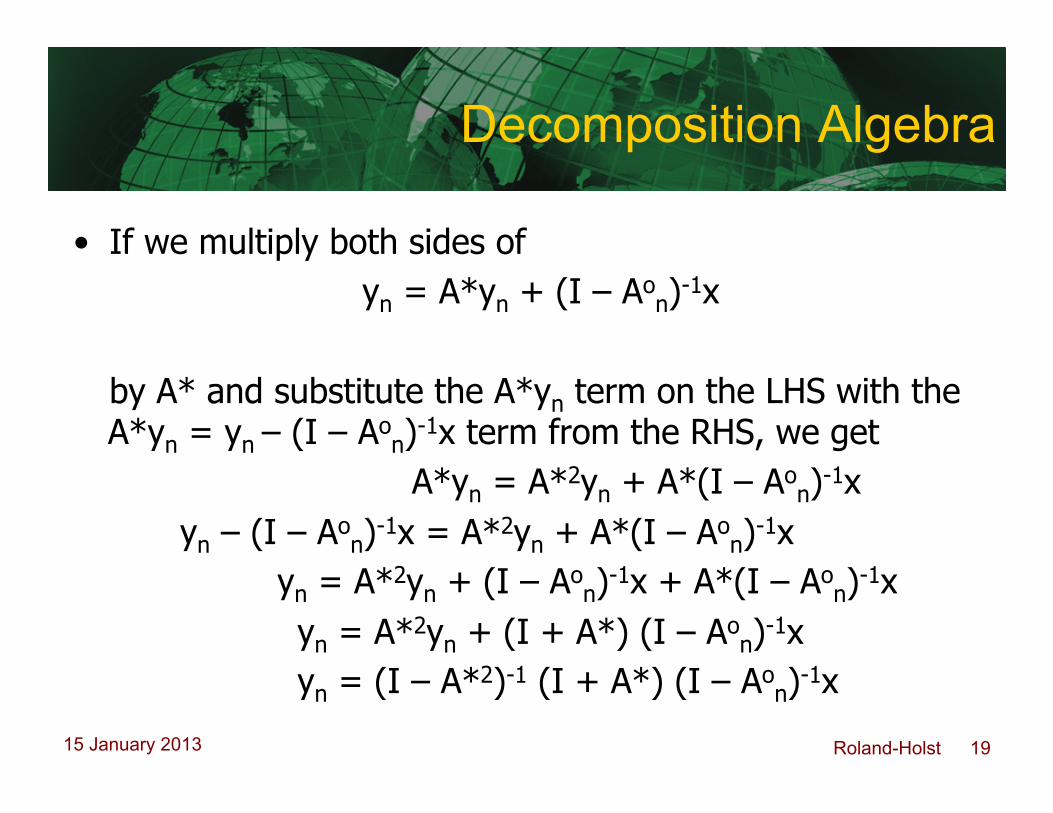
• If we multiply both sides of yn = A*yn + (I – Ao
n)-1x by A* and substitute the A*yn term on the LHS with the A*yn = yn – (I – Ao
n)-1x term from the RHS, we get A*yn = A*2yn + A*(I – Ao
n)-1x yn – (I – Ao
n)-1x = A*2yn + A*(I – Aon)-1x
yn = A*2yn + (I – Aon)-1x + A*(I – Ao
n)-1x yn = A*2yn + (I + A*) (I – Ao
n)-1x yn = (I – A*2)-1 (I + A*) (I – Ao
n)-1x
Roland-Holst 20 15 January 2013
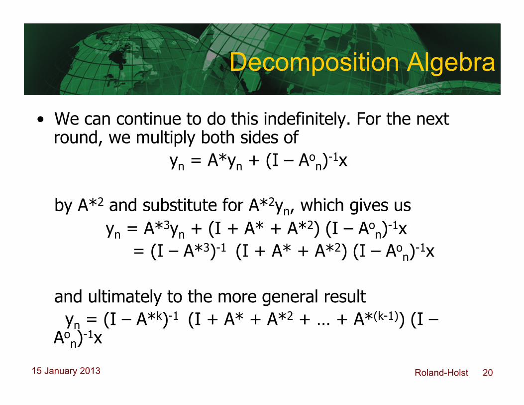
Decomposition Algebra
• We can continue to do this indefinitely. For the next round, we multiply both sides of yn = A*yn + (I – Ao
n)-1x
by A*2 and substitute for A*2yn, which gives us yn = A*3yn + (I + A* + A*2) (I – Ao
n)-1x = (I – A*3)-1 (I + A* + A*2) (I – Ao
n)-1x
and ultimately to the more general result yn = (I – A*k)-1 (I + A* + A*2 + … + A*(k-1)) (I – Ao
n)-1x
Roland-Holst 21 15 January 2013
Decomposition Algebra
• While we could do decomposition indefinitely, we typically stop at k = 3 steps because 3 is the number of endogenous accounts within the SAM. In other words, the flow of income around the SAM undergoes 3 steps.
Roland-Holst 22 15 January 2013
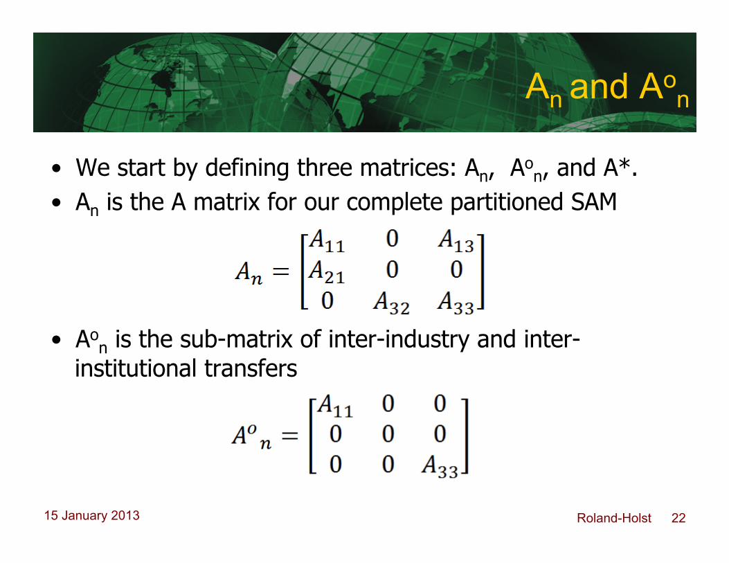
An and Aon
• We start by defining three matrices: An, Aon, and A*.
• An is the A matrix for our complete partitioned SAM
• Aon is the sub-matrix of inter-industry and inter-
institutional transfers
Roland-Holst 23 15 January 2013
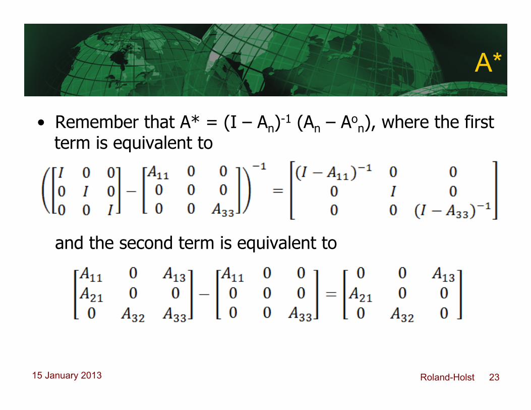
A*
• Remember that A* = (I – An)-1 (An – Aon), where the first
term is equivalent to
and the second term is equivalent to
Roland-Holst 24 15 January 2013
A*
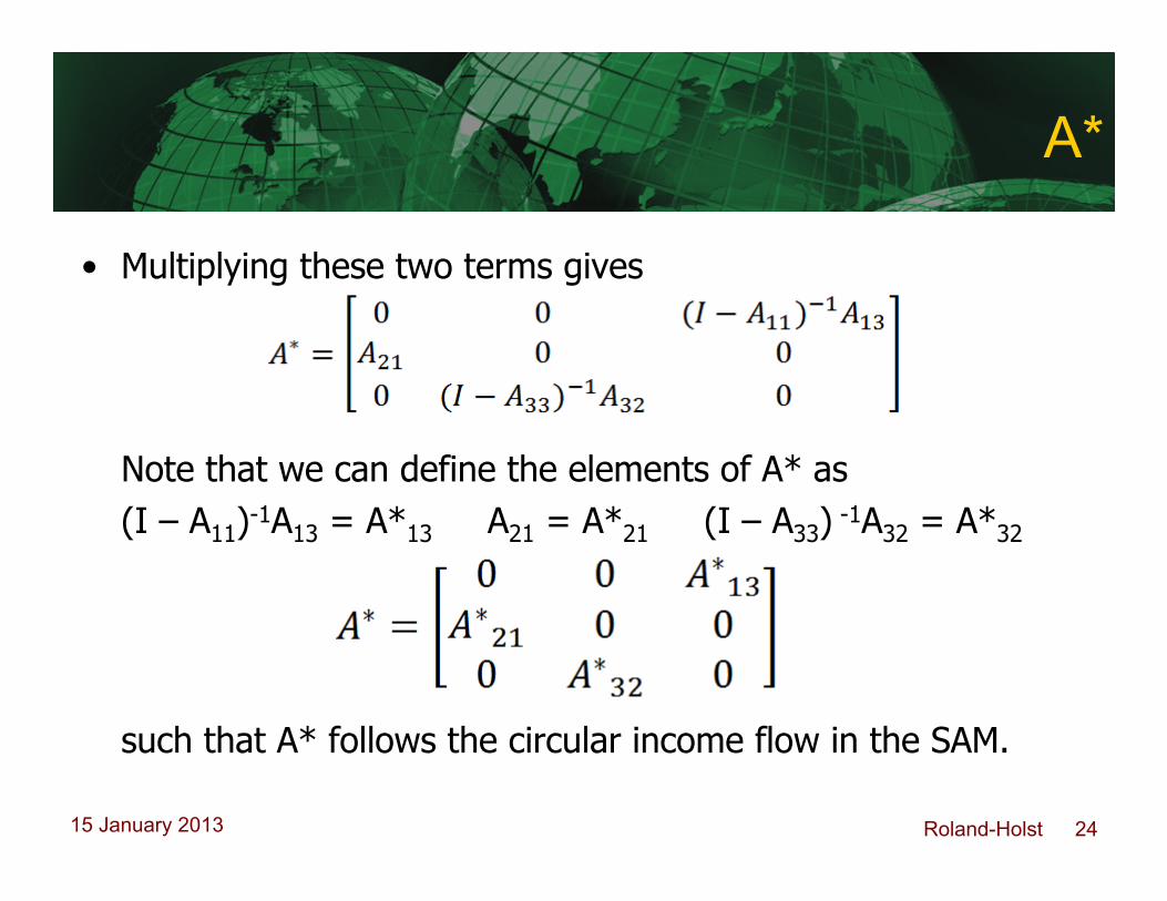
• Multiplying these two terms gives
Note that we can define the elements of A* as (I – A11)-1A13 = A*13 A21 = A*21 (I – A33) -1A32 = A*32
such that A* follows the circular income flow in the SAM.
Roland-Holst 25 15 January 2013
Ma3Ma2Ma1
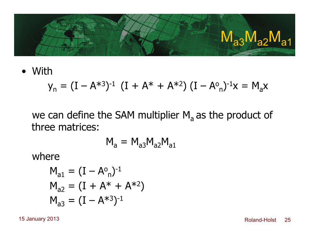
• With yn = (I – A*3)-1 (I + A* + A*2) (I – Ao
n)-1x = Max we can define the SAM multiplier Ma as the product of three matrices: Ma = Ma3Ma2Ma1 where Ma1 = (I – Ao
n)-1 Ma2 = (I + A* + A*2) Ma3 = (I – A*3)-1
Roland-Holst 26 15 January 2013
Ma1
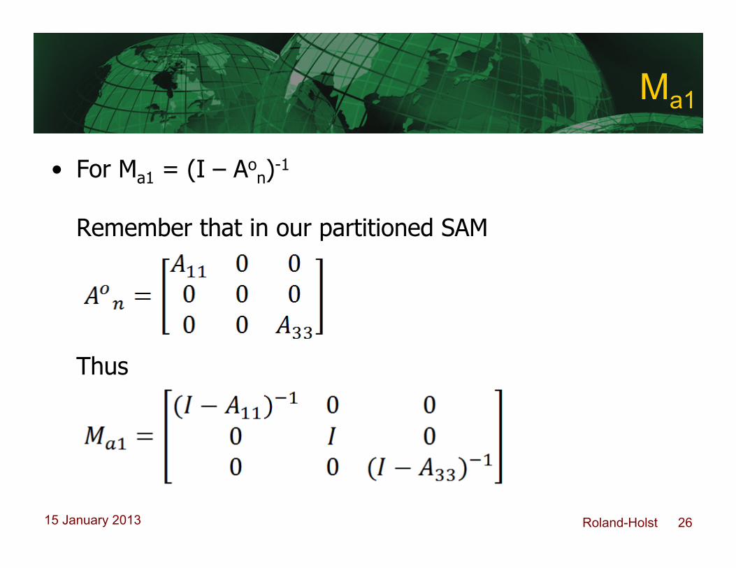
• For Ma1 = (I – Aon)-1
Remember that in our partitioned SAM
Thus
Roland-Holst 27 15 January 2013
Ma1
• From the (I-A11)-1 and (I-A33)-1 elements of Ma1 you can begin to develop some intuition about how to interpret the decomposed multipliers.
• Ma1 is typically referred to as the transfers, or direct effects, multiplier, because it captures the multiplier effects of transfers within accounts; in this case industries, i.e. (I-A11)-1, and institutions, i.e. (I-A33)-1.
• Ma1 only captures within account effects; it tells us nothing about factors or institutions.
Roland-Holst 28 15 January 2013
Ma2
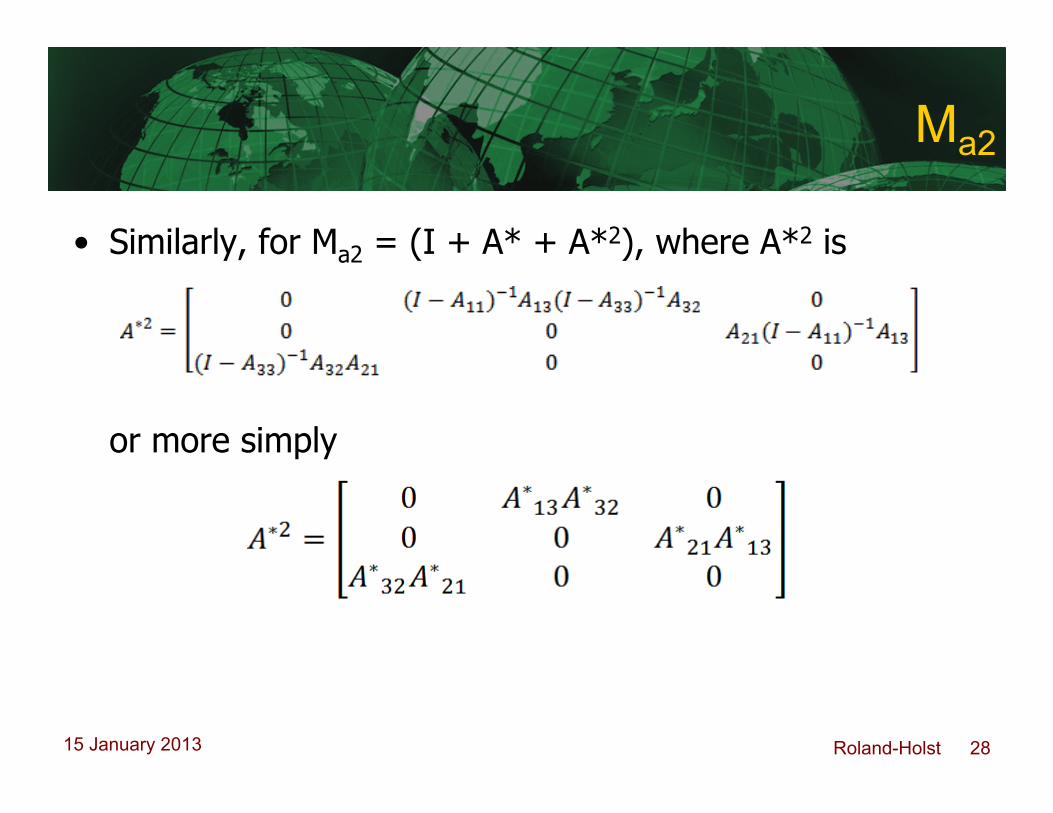
• Similarly, for Ma2 = (I + A* + A*2), where A*2 is
or more simply
Roland-Holst 29 15 January 2013
Ma2
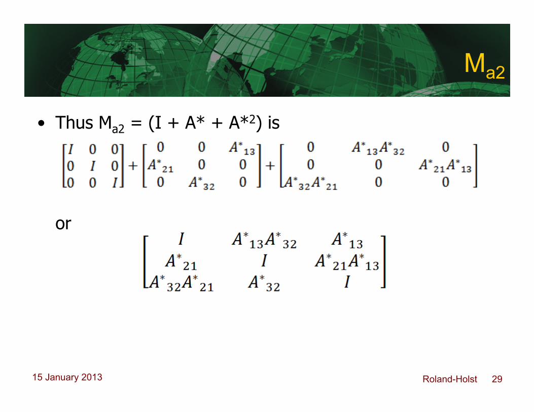
• Thus Ma2 = (I + A* + A*2) is
or
Roland-Holst 30 15 January 2013
Ma2
• Ma2 is the only matrix with off-diagonal elements, and is referred to as the cross-effects, or open-loop, multiplier.
• Ma2 captures the effects of an injection into the system as it moves through the system without coming back to its origin (hence the name ‘open-loop’). In other words, Ma2 shows how an external injection travels from endogenous demand to income (“across” institutions), but not from income to demand.
Roland-Holst 31 15 January 2013
Ma3
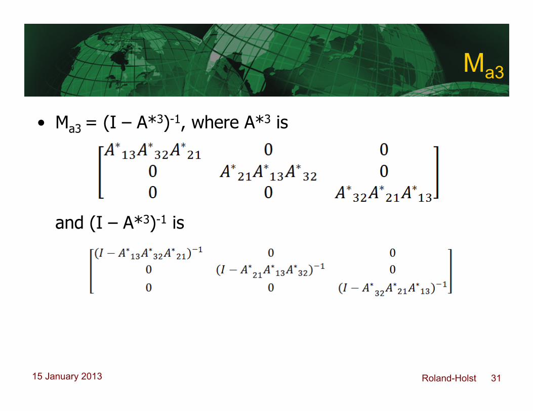
• Ma3 = (I – A*3)-1, where A*3 is
and (I – A*3)-1 is
Roland-Holst 32 15 January 2013
Ma3
• Ma3 is typically referred to as the circular, or closed loop, multiplier.
• Ma3 captures the full circular effects of an exogenous income injection on one account, once the circular flow of income returns to the account where the injection took place.
• In other words, Ma3 represents the full circular multiplier effects net of Ma1 and Ma2.
Roland-Holst 33 15 January 2013
Additive Multipliers
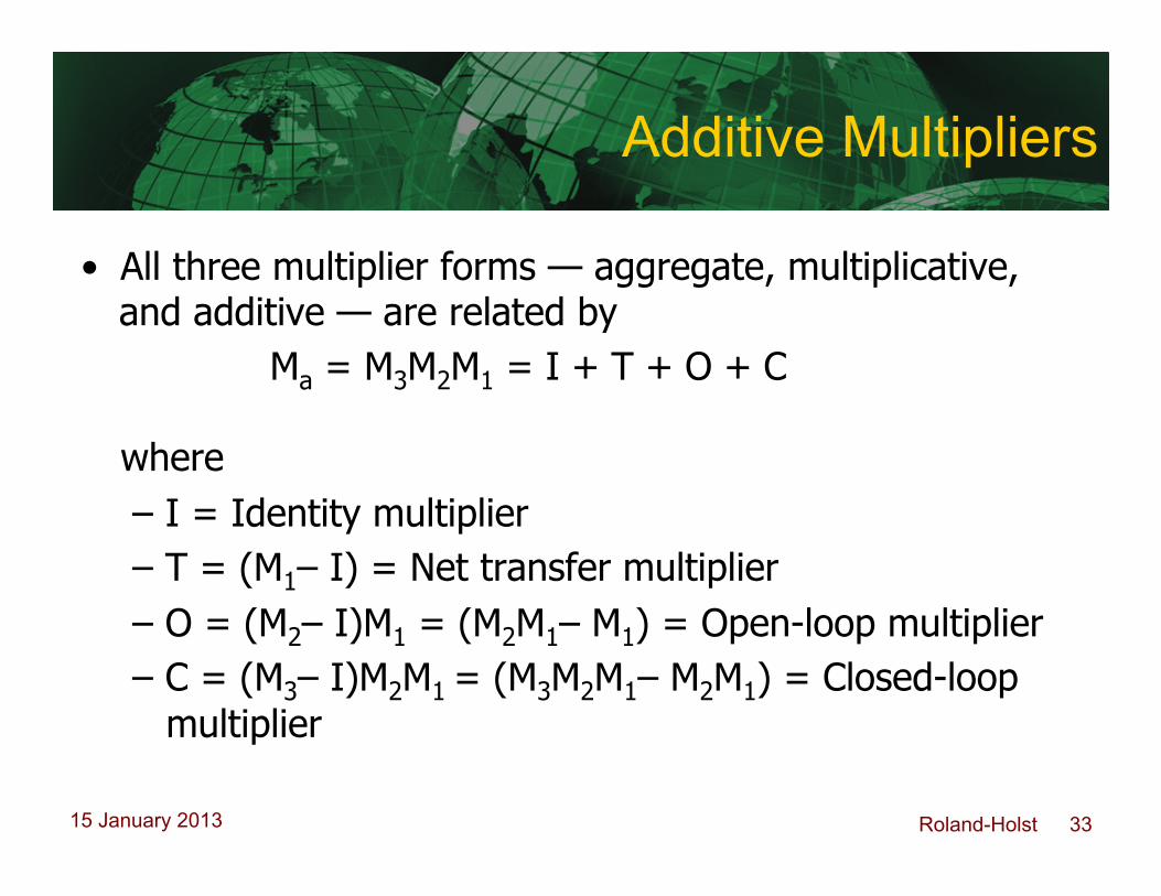
• All three multiplier forms — aggregate, multiplicative, and additive — are related by Ma = M3M2M1 = I + T + O + C
where – I = Identity multiplier – T = (M1– I) = Net transfer multiplier – O = (M2– I)M1 = (M2M1– M1) = Open-loop multiplier – C = (M3– I)M2M1 = (M3M2M1– M2M1) = Closed-loop
multiplier
Roland-Holst 34 15 January 2013
Applications
• Standard multiplier decomposition presents an interesting way of separating out the structural effects of exogenous shocks.
• For instance, in their study of Sri Lanka Pyatt and Round (1979) found that transfer multipliers were significantly lower than open-loop (between-account) multipliers, suggesting the need for a more comprehensive approach to understanding income flows.
Roland-Holst 35 15 January 2013
Regional Multiplier Decomposition
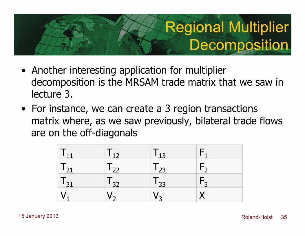
• Another interesting application for multiplier decomposition is the MRSAM trade matrix that we saw in lecture 3.
• For instance, we can create a 3 region transactions matrix where, as we saw previously, bilateral trade flows are on the off-diagonals
T11 T12 T13 F1 T21 T22 T23 F2 T31 T32 T33 F3 V1 V2 V3 X

Roland-Holst 36 15 January 2013
Regional Multiplier Decomposition
• Using the transactions sub-matrix
we can examine regional trade multipliers through the same approach as above, although in this case our Ao
n matrix would include T11, T22, and T33 along its block diagonal.
T11 T12 T13 F1 T21 T22 T23 F2 T31 T32 T33 F3 V1 V2 V3 X
Roland-Holst 37 15 January 2013
Regional Multiplier Decomposition
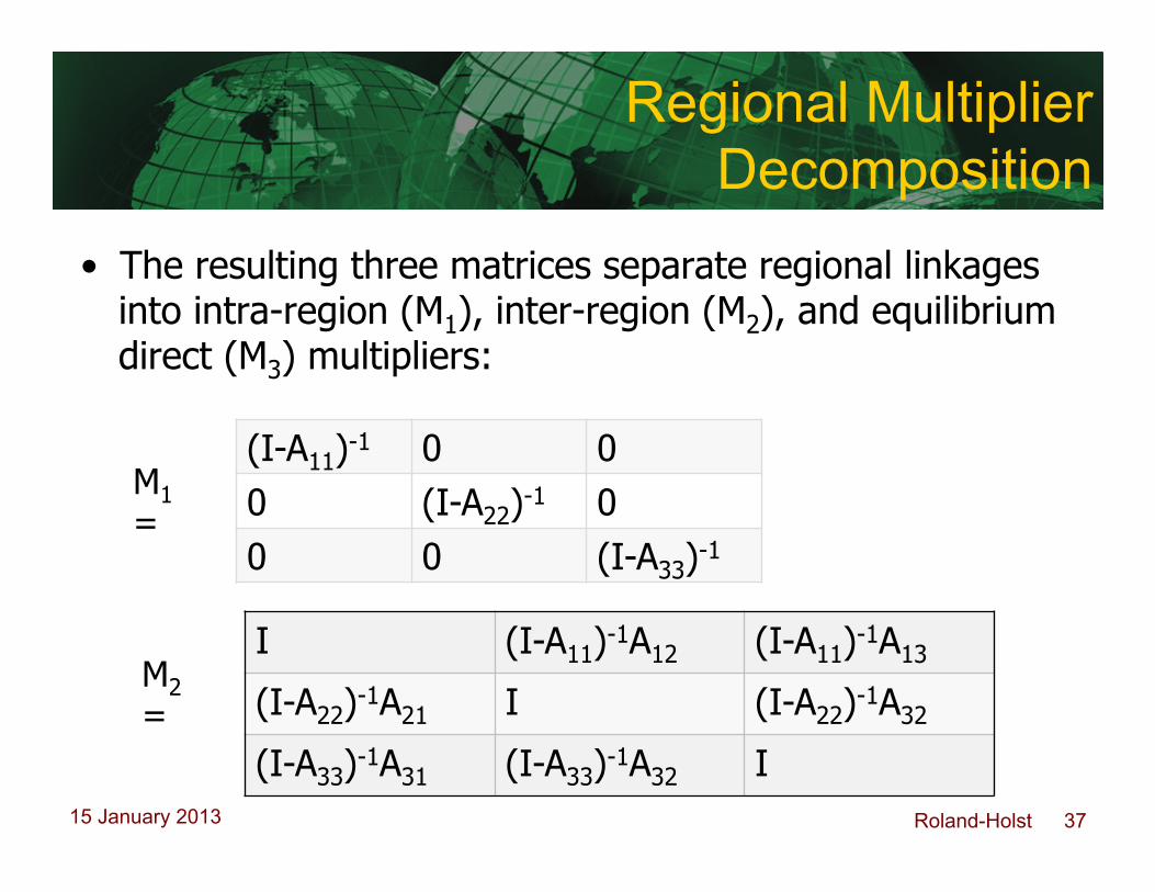
• The resulting three matrices separate regional linkages into intra-region (M1), inter-region (M2), and equilibrium direct (M3) multipliers:
(I-A11)-1 0 0 0 (I-A22)-1 0 0 0 (I-A33)-1
M1 =
M2 =
I (I-A11)-1A12 (I-A11)-1A13
(I-A22)-1A21 I (I-A22)-1A32
(I-A33)-1A31 (I-A33)-1A32 I
Roland-Holst 38 15 January 2013
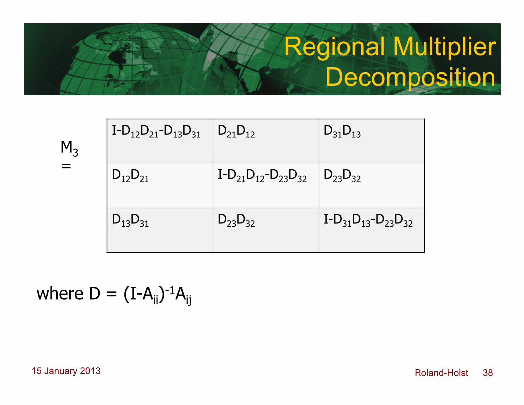
Regional Multiplier Decomposition
where D = (I-Aii)-1Aij
I-D12D21-D13D31 D21D12
D31D13
D12D21 I-D21D12-D23D32 D23D32
D13D31 D23D32 I-D31D13-D23D32
M3 =