Fantastic: Feature ANalysis Technology AccessingSTatistics (In a Corpus): Technical Report v1.5

Daniel Mullensiefen

June 19, 2009

Contents

1 Introduction 4

2 Input format 4

3 Running the program 53.1 Computing features of melodies . . . . . . . . . . . . . . . . . . . . . . . . 63.2 Computing frequencies of melody features in the context of a melody corpus 73.3 Computing features on the occurrence of m-types in the context of a melody

corpus . . . . . . . . . . . . . . . . . . . . . . . . . . . . . . . . . . . . . . 93.4 Computing similarities between melodies based on features . . . . . . . . . 10

4 Overview 114.1 Global architecture . . . . . . . . . . . . . . . . . . . . . . . . . . . . . . . 114.2 Global parameters . . . . . . . . . . . . . . . . . . . . . . . . . . . . . . . 11

5 Basic representation of melodic data 13

6 Features based on the content of a single melody 136.1 Feature Value Summary Statistics . . . . . . . . . . . . . . . . . . . . . . . 13

6.1.1 Descriptive statistics on pitch . . . . . . . . . . . . . . . . . . . . . 136.1.2 Descriptive statistics on pitch intervals . . . . . . . . . . . . . . . . 146.1.3 Descriptive statistics on note durations . . . . . . . . . . . . . . . . 156.1.4 Global extension . . . . . . . . . . . . . . . . . . . . . . . . . . . . 166.1.5 Melodic Contour . . . . . . . . . . . . . . . . . . . . . . . . . . . . 176.1.6 Implicit Tonality . . . . . . . . . . . . . . . . . . . . . . . . . . . . 21

6.2 m-type Summary Statistics . . . . . . . . . . . . . . . . . . . . . . . . . . . 226.2.1 Creating m-types . . . . . . . . . . . . . . . . . . . . . . . . . . . . 236.2.2 Computing m-type summary statistics . . . . . . . . . . . . . . . . 24

1

7 Corpus-based Feature Statistics 257.1 Frequencies of Summary Features . . . . . . . . . . . . . . . . . . . . . . . 25

7.1.1 Frequency Densities for numerical continuous features . . . . . . . . 267.1.2 Relative frequencies for categorical features . . . . . . . . . . . . . . 277.1.3 Relative frequencies for numerical discrete features . . . . . . . . . 27

7.2 Features derived from m-type distributions in melody and corpus . . . . . 287.2.1 Comparisons between m-type distributions from melody and corpus 287.2.2 Features derived from m-type corpus frequencies . . . . . . . . . . . 297.2.3 Features derived from m-type melody frequencies and inverted m-

type corpus frequencies . . . . . . . . . . . . . . . . . . . . . . . . . 307.2.4 Features derived from entropy-based weightings . . . . . . . . . . . 31

8 Similarity computation based on features and feature distributions 328.1 Methods for computing similarities from features . . . . . . . . . . . . . . 32

8.1.1 Euclidean Distance / Similarity . . . . . . . . . . . . . . . . . . . . 328.1.2 Similarity based on Gower’s coefficient . . . . . . . . . . . . . . . . 338.1.3 Corpus-based similarity . . . . . . . . . . . . . . . . . . . . . . . . 33

2

Version History

May 2009 Version 1.0 Describes three main functions: compute.features(),compute.corpus.based.feature.frequencies(),compute.m.type.corpus.based.features().The latter is still very slow.

June 2009 Version 1.5 Describes new main function feature.similarity().

3

1 Introduction

Fantastic is a program, written in R 1, that analyses melodies by computing features.The aim is to characterise a melody or a melodic phrase by a set of numerical or categor-ical values reflecting different aspects of musical structure. This feature representation ofmelodies can then be applied in Music Information Retrieval algorithms or computationalmodels of melody cognition. Apart from characterising melodies individually by featurevalues, Fantastic also allows for similarity comparisons between melodies that are basedon feature computation.

Similarly to existing melody analysis tools (e.g. the MIDI tool box, Eerola and Toivi-ainen (2004)), the feature computation algorithms in Fantastic make use of ideas andconcepts from descriptive statistics, music theory, and music cognition. But in contrastto most existing software, Fantastic also incorporates approaches derived from compu-tational linguistics and provides the option to characterise a melody by a set of featureswith respect to a particular corpus of melodies.

The idea of characterising and analysing melodies in terms of features is not new andowes much to great predecessors in the work of, for example, Lomax (1977), Steinbeck(1982), Jesser (1990), Sagrillo (1999), Eerola and Toiviainen (2004). Introductions to theconcept of feature-based melody analysis and examples of the application of this conceptin Ethnomusicology, Musicology, Music Psychology, and Music Information Retrieval canbe found in those publications.

This technical report documents the internal processing structure of Fantastic as wellas the features currently implemented.

2 Input format

Fantastic uses symbolic representations of monophonic melodies as melodic input data.It accepts MCSV files (Frieler, 2005) which also are the input format to the melodic similar-ity computation program Simile by Klaus Frieler (Mullensiefen and Frieler, 2006). MCSVfiles are similar to kern files in that they represent musical events in a tabular way but areconceptually simpler and more limited (e.g. cannot handle polyphony yet). Subsequentlines in the MCSV file represent note events in the order appear in the melody and thedifferent columns contain different information about the note events. The most importanttypes of information are pitch (represented as MIDI number), note onset in seconds, noteonset in metrical time, note duration (in metrical time and in seconds), and phrase bound-ary (binary information for every note event: 1 indicated that note is a phrase boundary, 0means note is not a boundary). Currently Temperley’s Grouper (Temperley, 2001) is usedas melody segmentation algorithm, column Tempe in MCSV file).

MCSV files can be created by using Klaus Frieler’s melody conversion program Mel-conv. Currently Melconv enables conversion between a number of symbolic musicformats such as MIDI, the Essener Assoziativ Code (EsAC), notes (Temperley, 2001), and

1 see http://www.r-project.org

4

MCSV. But since they are ordinary text files with a tabular format it is easy to createMCSV files from most melody processing software.

3 Running the program

The source code of Fantastic comprises five .R files2 which are packaged together andavailable online3. They need to be unpacked and placed into the same directory, preferablythe working directory of the R-analysis. Fantastic makes use of the following, non-standard R-packages which have to be installed before running the program: MASS andzipfR.

Currently, there are three top-level functions4 for computing features and feature fre-quencies from melodies encoded in MCSV files:

1. compute.features: Computes feature summary statistics and m-type summarystatistics for a melodies given as a list of MCSV files. This includes features onthe pitches, intervals, and rhythmic durations of a melody as well as features sum-marising the contour and the harmonic content. In addition, features characterisingthe repetitiveness of short melodic-rhythmic elements (which we call m-types seesection 6.2) in a melody are also computed.

2. compute.corpus.based.feature.frequencies: For each melody, this function com-putes the density or relative frequency of the summary features with respect to thedistribution of summary features in a specified corpus. That is, for each melody eachfeature value is replaced by its corresponding frequency value from the frequencydistribution of a corpus. Thus, this computation makes a step from the feature scaleto a commonness vs. rarity scale. The input to this function has therefore twomain components: A list of analysis melodies for each of which frequency valuesare computed and a corpus of melodies from which the frequency distribution arederived.

3. compute.m.type.corpus.based.features: For each melody, this function com-putes features on the basis of how common or frequent the short melodic-rhythmicelements (m-types) are of which a melody is composed. This function has two maincomponents as input: A list of analysis melodies for each of which m-types are ex-tracted and a corpus of melodies from which the distribution of m-types is derived.

The three main functions are executed following three steps:

2 The five source files are names Fantastic.R, Feature Value Summary Statistics.R,M-Type Summary Statistics.R, Frequencies Summary Statistics.R, andM-Type Corpus Features.R.

3 http://www.doc.gold.ac.uk/isms/m4s/FANTASTIC.zip4 We are planning to integrate compute.corpus.based.feature.frequencies and

compute.m.type.corpus.based.features into a single function that computes information aboutmelodies in the context of a corpus.

5

1. Start the R installation on your computer and load the file Fantastic.R.

2. Preferably, make the directory that contains the .R source files and the MCSV filesfor analysis your working directory (setwd("<path to directory>")).

3. Call the either of the three functions with the appropriate argument val-ues (s. below) and assign an output object to it: e.g. output <-

compute.features(c("file1.csv", "file2.csv")).

3.1 Computing features of melodies

Function: compute.features(melody.filenames = list.files(path = dir,

pattern = ".csv"), dir = ".", output = "melody.wise", use.segmentation

= TRUE, write.out = FALSE)

Description: This is the main function for computing features of melodies encoded inMCSV files. This means that it computes features just for the melodies given, withoutany reference to a corpus of music, and returns a table containing feature values for eachmelody (or melodic phrase).

Arguments: The function compute.features takes the following arguments that con-trol the analysis procedure and have been set to default values in the current implementa-tion:

• melody.filenames: Takes the names of the files to be analysed. These can be eitherconcatenated with the function c(), (e.g. c("file1.csv", "file2.csv")) or youcan use the the R-function list.files() to list all the .csv files in the workingdirectory (list.files(pattern=".csv"). By default, all the .csv files found in thedirectory specified by dir are used as melody.filenames.

• dir: Takes the absolute path (starting with “/” or “\”) or relative path (startingwith any other symbol) to and name of the directory that contains the .csv filesfor analysis (e.g. “../analysis directory”). The default is the present workingdirectory. If the value(s) given to melody.filenames contain the directory path tothe files then the argument to dir is ignored.

• output takes the argument values "melody.wise" (default) and "phrase.wise".This arguments determines whether the analysis information in the output object isgiven for the melody as a whole or on the basis of the individual melodic phrases asindicated in the MCSV file (see above).

• use.segmentation takes argument values TRUE (default) and FALSE and determineswhether the feature computation is done on the melody as a whole or phrase byphrase.

6

• write.out takes argument values TRUE and FALSE (default) and determines whethera file with the analysis results should be written out.

The interactions between the arguments output and use.segmentation is specificallydefined for the following two cases:

• If use.segmentation is set to TRUE and output is set to "melody.wise" then nu-merical features are averaged over all phrases in the melody and the most frequentvalue of categorical features is computed as output.

• If use.segmentation is set to FALSE and output is set to "phrase.wise" then theprogram emits an error message and terminates because in order to output featureson a phrase-level the program has to make use of segmentation information.

Output: The output is a table (i.e. an R-data frame) that has as lines the datafor each melody analysed (or the data for each phrase of each melody analysed ifoutput="phrase.wise" is requested). The columns of the output table comprise file name(and phrase number) as well as analytic features that Fantastic computes. These can benumeric feature values or feature labels as character strings. For all melodies and melodyphrase for which feature values cannot be computed (e.g. because the length of a phraseis outside the phrase length limits as given as a global parameter to the program see 4.2),then NAs are written out as features values for that phrase.5

3.2 Computing frequencies of melody features in the context ofa melody corpus

Function: compute.corpus.based.feature.frequencies(analysis.melodies

= "analysis dir", ana.dir = "analysis melodies", corpus = "corpus dir",

write.out.corp.freq = TRUE, comp.feat.use.seg = TRUE, comp.feat.output =

"phrase.wise")

Description: This is the main function for computing the frequencies of features ofmelodies (the analysis melodies) in the context of a corpus of melodies. It returns a tablecontaining frequency values for each analysis melody (or each melodic phrase).

Arguments: compute.corpus.based.feature.frequencies is run with the followingarguments and default settings:

• analysis.melodies: Takes either a feature file as produced by compute.features

and ending in “.txt” or a list of MCSV files or a directory name (including path) inwhich the melodies for analysis can be found. The default is a directory with name“analysis dir” that is below the present working directory.

5 For technical reasons and as an exception, if feature values cannot be computed for the first phraseof an analysis melody, then this phrase is skipped and no NAs are written out.

7

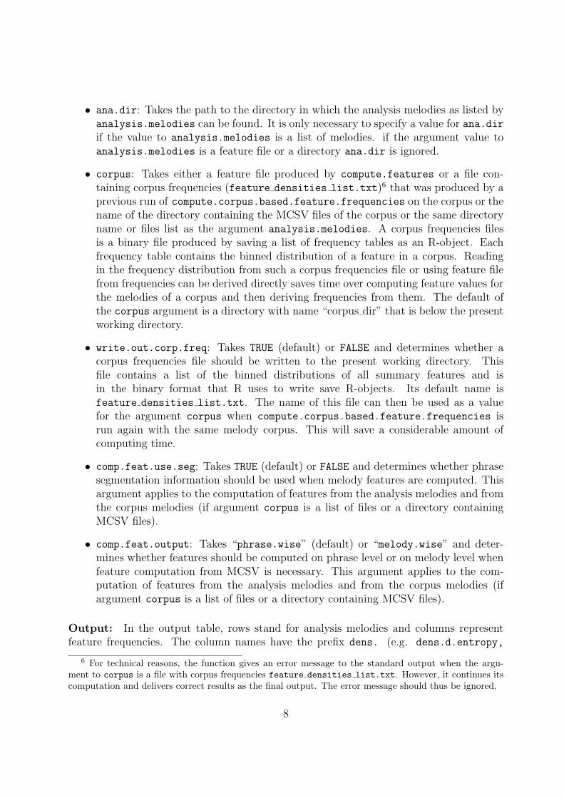
• ana.dir: Takes the path to the directory in which the analysis melodies as listed byanalysis.melodies can be found. It is only necessary to specify a value for ana.dirif the value to analysis.melodies is a list of melodies. if the argument value toanalysis.melodies is a feature file or a directory ana.dir is ignored.

• corpus: Takes either a feature file produced by compute.features or a file con-taining corpus frequencies (feature densities list.txt)6 that was produced by aprevious run of compute.corpus.based.feature.frequencies on the corpus or thename of the directory containing the MCSV files of the corpus or the same directoryname or files list as the argument analysis.melodies. A corpus frequencies filesis a binary file produced by saving a list of frequency tables as an R-object. Eachfrequency table contains the binned distribution of a feature in a corpus. Readingin the frequency distribution from such a corpus frequencies file or using feature filefrom frequencies can be derived directly saves time over computing feature values forthe melodies of a corpus and then deriving frequencies from them. The default ofthe corpus argument is a directory with name “corpus dir” that is below the presentworking directory.

• write.out.corp.freq: Takes TRUE (default) or FALSE and determines whether acorpus frequencies file should be written to the present working directory. Thisfile contains a list of the binned distributions of all summary features and isin the binary format that R uses to write save R-objects. Its default name isfeature densities list.txt. The name of this file can then be used as a valuefor the argument corpus when compute.corpus.based.feature.frequencies isrun again with the same melody corpus. This will save a considerable amount ofcomputing time.

• comp.feat.use.seg: Takes TRUE (default) or FALSE and determines whether phrasesegmentation information should be used when melody features are computed. Thisargument applies to the computation of features from the analysis melodies and fromthe corpus melodies (if argument corpus is a list of files or a directory containingMCSV files).

• comp.feat.output: Takes “phrase.wise” (default) or “melody.wise” and deter-mines whether features should be computed on phrase level or on melody level whenfeature computation from MCSV is necessary. This argument applies to the com-putation of features from the analysis melodies and from the corpus melodies (ifargument corpus is a list of files or a directory containing MCSV files).

Output: In the output table, rows stand for analysis melodies and columns representfeature frequencies. The column names have the prefix dens. (e.g. dens.d.entropy,

6 For technical reasons, the function gives an error message to the standard output when the argu-ment to corpus is a file with corpus frequencies feature densities list.txt. However, it continues itscomputation and delivers correct results as the final output. The error message should thus be ignored.

8

dens.h.contour) in order to distinguish them from similarly named columns containingthe values of the corresponding features. This table is automatically written to a file nameddensities of feature values.txt.

3.3 Computing features on the occurrence of m-types in the con-text of a melody corpus

Function: compute.m.type.corpus.based.features(analysis.melodies, ana.dir

=".", corpus, corpus.dir = ".")

Description: This is the main function for computing features that informs about them-types occurring in a melody in the context of a corpus. Its usage follows the basically thesame logic as compute.corpus.based.feature.frequencies and its main input compo-nents are a set of analysis melodies and a corpus of melodies. It returns a table containingm-type corpus features for each analysis melody (or melodic phrase).

Arguments: compute.m.type.corpus.based.features is run with the following argu-ments and default settings:

• analysis.melodies: Takes a list of files for which the m-type occurrence feature areto be computed.

• ana.dir: Takes the directory name (path) in which the analysis melodies are to befound. The default is the present working directory (“.”).

• corpus: Takes either the name of a m-type frequency file ending in “.txt” or a a listof files or the same list of files as the argument analysis.melodies.

• corpus.dir: Takes either the name of the directory in which the melodies of thecorpus are to be found or the same value as the argument ana.dir. The default isthe present working directory (“.”).

Output: The output of this function is a table where each row represents oneanalysis melody and columns stand for m-type occurrence features. Columnnames are prefixed with “mtcf.” (= m-type corpus feature) to distinguish themform the m-type features that are computed from compute.features. The re-sults are also written to a file named mtype corpus based feat.txt. With everyrun compute.m.type.corpus.based.features writes out an m-type frequency file con-taining the m-types and their frequencies for every melody in the corpus is writ-ten to the present working directory. This m-type frequency file has the namem-type counts several melodies.txt. Using this files as an argument to corpus insubsequent runs of compute.m.type.corpus.based.features with the same corpus in-formation will save a considerable amount of computing time. A warning message occurs

9

on standard output during the computation of some rank correlations if all m-types occurwith the same frequency and have thus the same rank.The full output is still computedand the warning message can be ignored.

3.4 Computing similarities between melodies based on features

Function: feature.similarity(mel.fns=list.files(path=dir,pattern=".csv"),

dir=".", features=c("p.range","step.cont.glob.var","tonalness","d.eq.trans"),

use.segmentation=FALSE, method="euclidean", eucl.stand=TRUE,

corpus.dens.list.fn=NULL, average=TRUE)

Description: This is the main function for computing similarity values between melodies.It computes features using the function compute.features underneath and offers threedifferent methods how similarity values can be derived from the feature values of twomelodies. It takes a list of melodies as input and its output is a similarity matrix containingsimilarity values for all (symmetric) pairwise comparisons possible for the melodies givenas input.

Arguments: compute.features is run with the following arguments:

• mel.fns: Takes a list of MCSV files for which pairwise similarities should be com-puted. By default, all the .csv files found in the directory specified by argument dirare used as mel.fns. The files must contain segmentation information even if it notused in the computation.7

• dir: Takes the directory names (path) in which the input files are to be found. Thedefault is the present working directory (“.”).

• features: Takes a character vector of feature names on the basis ofwhich similarities should be computed. Currently, only features de-scribed in 6.1 are allowed. The default is rather arbitrarily set toc("p.range","step.cont.glob.var","tonalness","d.eq.trans"). If the valueto argument method is ‘‘euclidean" only numerical features can be used, i.e.thecategorical features h.contour, mode, and int.contour.class are not allowed.

• use.segmentation: Takes TRUE or FALSE (the default) as input and determineswhether phrase segmentation information should be used by compute.features tocompute the feature values for each melody.

• method: Takes a character string to determine the method which should be used toderive similarity values from from the feature values of each melody. The methodmust be one of ‘‘euclidean" (the default), ‘‘gower" or ‘‘corpus".

7 Unfortunately, the function doesn‘t currently accept a feature data.frame as input, such as the outputof compute.features(). Therefore, the feature computation has to be run again with every call tofeature.similarity(), even if it is on a set of melodies that has been used as input previously.

10

• eucl.stand: Takes either TRUE or FALSE (the default) and determines whetherfeatures values should be standardised over all input melodies when euclidean isthe value of argument ‘‘method". The standardisation used is the so-called z-standardisation (subtraction of feature mean and division by feature variance).

• corpus.dens.list.fn: Takes filename and path of a file containing in-formation about the frequency distributions of features in a corpus (de-fault file name: feature densities list.txt) as produced by the functioncompute.corpus.based.feature.frequencies. This corpus information is onlyused when the value to argument ‘‘method" is ‘‘corpus".

• average: Takes the values TRUE (the default) or FALSE and determines whether themean of the similarity values based on different features should be taken. If FALSE

one similarity matrix for each feature is outputted.

Output: The output of this function is a list of similarity matrices. Each matrix is an R-object of class dist and is of size (n−1)2 where n is the number of melodies given as input.Only the lower triangle of each matrix is fully (no diagonal). Note that while the matrixis of class dist, the values represent similarities on a scale from 0 (minimum similarity)to 1 (maximal similarity / identity). In order to obtain a distance matrix that could beused as input to existing R-functions, such as hclust(), the matrix has to be transformedfirst by subtracting it from 1, e.g. dist.matrix <- 1 - sim.matrix. When the input toargument feature is more than 1 feature and the value of argument average is FALSE,then the output is a list of similarity matrices, one for each feature. A conversion fromthis matrix of class dist to a normal n × n matrix can be achieved using the R-functionas.matrix().

4 Overview

4.1 Global architecture

The global architecture is displayed graphically in the processing flow chart ??.

4.2 Global parameters

Fantastic operates on the basis of a few global parameters.

1. phr.length.limits <- c(2, 24): Is a vector of length 2 that holds the lower andupper limit of the length of a phrase. Defaults are 2 and 24.

2. int.class.scheme: Is a data frame that holds pitch intervals (in semitones) andcorresponding interval classes (represented as 2-digit sequences of letters and num-bers). This pitch interval classification scheme is used for constructing the so-called

11

m-types (see section 6.2). The default classification scheme is summarised in table1:

Interval in semitones Interval Class Value-12 d8-11 d7-10 d7-9 d6-8 d6-7 d5-6 dt- 5 d4-4 d3-3 d3-2 d2-1 d20 s11 u22 u23 u34 u35 u46 ut7 u58 u69 u610 u711 u712 u8

Table 1: Interval classification scheme for construction of m-types

3. tr.class.scheme: Is a list of two vectors. The first vector holds the labels for threerelative rhythm classes (represented as 1-letter strings). Defaults are class.symbols= c("q", "e", "t"). The second vector has the two upper limits of rhythmclass 1 and 2 (represented as numeric time ratios). Defaults are upper.limits =

c(0.8118987, 1.4945858). This duration ratio classification scheme is used forconstructing the so-called m-types (see section 6.2).

4. n.limits <- c(1, 5): Is a vector of length 2 that holds the lower and the upperlimit of the length of the m-types to be used for analysis (see section 6.2). Defaultsare 1 and 5.

12

5 Basic representation of melodic data

In a similar way to the MCSV file format (see section 2), Fantastic represents a melodyinternally as a sequence of notes which are represented as tuples of time and pitch infor-mation:

ni = (ti, pi)

The basic unit of pitch information is always MIDI pitch while the basic unit of timeinformation is expressed in milliseconds as a unit of absolute time and as the smallestmetrical unit occurring in a given melody which we will call tatum in the remainder of thisdocument.8 Whether timing information expressed in milliseconds or tatums depends onthe purpose and technical construction of the feature it is used in. The MCSV file providesboth types of information.

6 Features based on the content of a single melody

6.1 Feature Value Summary Statistics

The functions for computing Feature Value Summary Statistics can be foundin the file Feature Value Summary Statistics.R. The main function for comput-ing these features is summary.phr.features. As its first argument (phr.data)this function takes an R-dataframe having the same tabular structure asan MCSV file. For using the content of any MCSV file with this func-tion the user first has to load the content of the file into an R-object by:example.melody <- read.table(filename,sep=";",dec=",",skip=1,header=TRUE).Then example.melody can be the first argument to summary.phr.features. Thesecond argument (poly.contour) specifies whether features from the polynomial contourrepresentation ( 6.1.5) should be computed. Its default value is TRUE.

The features in this section use simple descriptive statistics on pitch, interval, andduration information of the melodies as well as some global features regarding melodyextension in time, melodic contour, and tonality.

6.1.1 Descriptive statistics on pitch

Feature 1 (Pitch Range: p.range)

p.range = max(p)−min(p) (1)

8 The term tatum was invented in computational music analysis by (Bilmes, 1993, footnote p. 21) todenote the high frequency pulse or smallest metrical unit that can be perceived in a piece. Before thisconcept was appropriated by computational musicology, it was used to describe the smallest division ofthe beat and used in the description of, for example, west-african music. The term for this concept variedbetween authors and was called density referent Hood (1971), elementary pulse Kubik (1998), or minimaloperational value Arom (1991). For a comparative discussion see Pfleiderer (2006).

13

Feature 2 (Pitch Standard Deviation: p.std)

p.std =

√∑Ni=1(pi − p)2

N − 1(2)

Feature 3 (Pitch Entropy: p.entropy) This is a variant of Shannon entropy (Shan-non, 1948). It is computed on the basis of the relative frequencies fi of the pitch classes piof a melody and normalised by maximum entropy given the upper phrase length limit as-sumed above (24).9 We denote the absolute frequency of pitch class i by Fi and the relativefrequency by fi.

fi =F (pi)∑i F (pi)

p.entropy = −∑

i fi · log2 filog2 24

(3)

6.1.2 Descriptive statistics on pitch intervals

Pitch intervals are derived from pitches by calculating the difference between two consec-utive pitches:

∆pi = pi+1 − piIn addition to raw intervals that have magnitude and direction information, features arealso computed on the absolute intervals of a melody which are only characterised by theirmagnitude:

|∆pi|

Feature 4 (Absolute Interval Range: i.abs.range)

i.abs.range = max(|∆p|)−min(|∆p|) (4)

Feature 5 (Mean Absolute Interval: i.abs.mean)

i.abs.mean =

∑i |∆pi|N

(5)

where N is the length of the interval vector ∆p.

9 Note that the standard way of normalising entropy is by diving by the maximum entropy as given bythe log of the size of the symbol alphabet - in this case the pitch alphabet. Unfortunately, it can not beknown in advance what size of the pitch alphabet is for any given set of melodies. However, empirically,the length of a melody correlates quite strongly with its entropy and therefore it seemed reasonable tostandardise entropy by the maximum phrase length that is given to the program as a global parameter.Thus, the maximum entropy is here assumed to be the entropy of a melody with maximum phrase lengththat has a different pitch class value for each note.

14

Feature 6 (Standard Deviation Absolute Interval: i.abs.std)

i.abs.std =

√∑i(|∆pi| − |∆p|)2

N − 1(6)

Feature 7 (Modal Interval: i.mode) The modal interval is the most frequent intervalin a melody. In case that there is no single most frequent interval, the interval with thehighest (positive) number of semitones is chosen.10

Feature 8 (Interval Entropy: i.entropy) Inerval entropy is computed analogous topitch entropy but using log2 23 since the maximum number of different intervals given thephrase lengths limits is 23.

fi =F (∆pi)∑i F (∆pi)

i.entropy = −∑

i fi · log2 filog2 23

(7)

6.1.3 Descriptive statistics on note durations

Since the MCSV format does not represent rests adequately Fantastic represents notedurations as inter-onset intervals (IOIs). For durations in milliseconds we write ∆t andfor durations measured in metrical tatums we write ∆T . ∆t is used as a quasi-continuousrepresentation for durations and ∆T serves as a discrete numerical representation.

Feature 9 (Duration Range: d.range)

d.range = max(|∆t|)−min(|∆t|) (8)

Feature 10 (Median of Durations: d.median) The median of the distributions of amelody is the value of ∆T that divides the frequency distribution of discrete duration valuesinto two half with the same number of duration values (50%).

Feature 11 (Modal Duration: d.mode) The modal duration is the most frequent valueof ∆T . In case that there is no single most frequent value, the highest value of ∆T amongthe most frequent ones is chosen.

Feature 12 (Duration Entropy: d.entropy) Duration entropy is computed analogousto pitch and interval entropy, using log2 24 as the maximum entropy for normalisationgiven the upper phrase lengths limit of 24.

fi =F (∆Ti)∑n F (∆Ti)

10 Since typical interval distributions for tonal music show that larger intervals are much rarer thansmaller intervals, picking the largest most frequent pitch interval is a reasonable strategy to arrive adiscriminative and characteristic feature value.

15

d.entropy = −∑

i fi · log2 filog2 24

(9)

Feature 13 (Equal Duration Transitions: d.eq.trans) This feature as well the thetwo subsequent features are derived from features proposed by Steinbeck (1982, p. 152f)and measure the relative frequency of note duration transitions. First, duration ratiosbetween subsequent note durations as measured in tatums are computed and stored in avector R:

ri =∆Ti

∆Ti+1

Then, the relative number of subsequent duration ratio with equal value is counted whileappropriate rounding is applied to the duration ratio values. The sum is the divided by thetotal number of duration ratios of subsequent note, i.e. the length of the vector R.

d.eq.trans =

∑ri=1

1

|R|(10)

Feature 14 (Half Duration Transitions: d.half.trans) This features counts thenumber of note transitions where the first note is either twice as long or half as longas the second note, i.e. their duration ratio is either approximately 2 or 0.5.

d.half.trans =

∑ri=0.5∨ri=2

1

|R|(11)

Feature 15 (Dotted Duration Transitions: d.dotted.trans) This feature countsthe number of dotted note transitions, i.e. the first note has either a duration that isthree times as long as the second one or vice versa.

d.dotted.trans =

∑ri=

13∨ri=3

1

|R|(12)

6.1.4 Global extension

Feature 16 (Length: len) The length of a melody is the number of the notes it encom-passes.

Feature 17 (Global Duration: glob.duration) The global duration of a melody is de-fined as the difference between the onset of the last note and the onset of the first notemeasured in milliseconds.

glob.duration = tn − t1 (13)

16

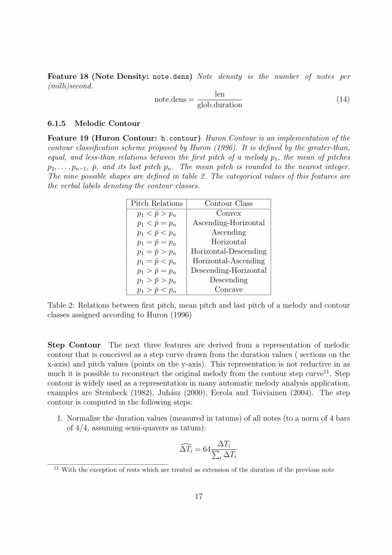
Feature 18 (Note Density: note.dens) Note density is the number of notes per(milli)second.

note.dens =len

glob.duration(14)

6.1.5 Melodic Contour

Feature 19 (Huron Contour: h.contour) Huron Contour is an implementation of thecontour classification scheme proposed by Huron (1996). It is defined by the greater-than,equal, and less-than relations between the first pitch of a melody p1, the mean of pitchesp2, . . . , pn−1, p, and its last pitch pn. The mean pitch is rounded to the nearest integer.The nine possible shapes are defined in table 2. The categorical values of this features arethe verbal labels denoting the contour classes.

Pitch Relations Contour Classp1 < p > pn Convexp1 < p = pn Ascending-Horizontalp1 < p < pn Ascendingp1 = p = pn Horizontalp1 = p > pn Horizontal-Descendingp1 = p < pn Horizontal-Ascendingp1 > p = pn Descending-Horizontalp1 > p > pn Descendingp1 > p < pn Concave

Table 2: Relations between first pitch, mean pitch and last pitch of a melody and contourclasses assigned according to Huron (1996)

Step Contour The next three features are derived from a representation of melodiccontour that is conceived as a step curve drawn from the duration values ( sections on thex-axis) and pitch values (points on the y-axis). This representation is not reductive in asmuch it is possible to reconstruct the original melody from the contour step curve11. Stepcontour is widely used as a representation in many automatic melody analysis application,examples are Steinbeck (1982), Juhasz (2000), Eerola and Toiviainen (2004). The stepcontour is computed in the following steps:

1. Normalise the duration values (measured in tatums) of all notes (to a norm of 4 barsof 4/4, assuming semi-quavers as tatum):

∆Ti = 64∆Ti∑i ∆Ti

11 With the exception of rests which are treated as extension of the duration of the previous note

17

2. Create a vector of length 64 by repeating each value of pi proportionally to its nor-malised duration ∆Ti.

Melodic step contour is then represented as a vector of length 64 with its elements beingsamples at equally-spaced positions of the raw pitch values of the melody.

Feature 20 (Step Contour Global Variation: step.cont.glob.var) This is definedas the standard deviation of the step contour vector x:

step.cont.glob.var =

√∑i(xi − x)2

N − 1(15)

Feature 21 (Step Contour Global Direction: step.cont.glob.dir) The step con-tour vector is correlated with the vector of bin numbers (n = 1, . . . , 64) and we definethe value of the Pearson-Bravais correlation coefficient to be the global direction of a stepcontour representation. The feature value has thus a value range from −1 to 1 which canbe interpreted as falling and rising contour shapes.

Feature 22 (Step Contour Local Variation: step.cont.loc.var) The local varia-tion in a step contour representation is captured as mean absolute difference between adja-cent values in the step contour vector x:

step.cont.loc.var =

∑N−1i=1 |xi+1 − xi|N − 1

(16)

Interpolation Contour The three following features are derived from a representationof melodic contour that is based on the idea of interpolating between the high and low points(i.e. contour turning points or contour extremum notes) of a melody using straight lines.This contour representation was formalised by Steinbeck (1982) and termed Polygonzug(= frequency polygon). Mullensiefen and Frieler (2004) discuss this representation underthe term Contourization. The idea of the definition of interpolation contour given hereis to substitute the pitch values of a melody with the sequence gradients that representthe direction and steepness of the melodic motion at evenly spaced points in time. Aninterpolation contour representation is obtained from the raw onset in milliseconds andpitch vaules by the following steps:

1. Determine all contour extremum notes. The contour extremum notes are the firstnote n1, the last note nN , and of every note ni inbetween, where ni−1 and ni+1 areeither both greater or both lower than ni, or in the cases where ni−1 or ni+1 are equalto ni but ni−2 and ni+1 or ni−1 or ni+2 are either both greater or both lower than ni.

2. As pure changing notes (notae cambiatae) generally do not make perceptually contourextrema, the changing notes are excluded from the set of potential contour extrema.A changing note ni is a note where the pitches of ni−1 and ni+1 or are equal. Thechanging notes are deleted from the set of contour extrema. This is a variant frominterpolation contour definition given by Mullensiefen and Frieler (2004).

18

3. Calculate the gradients of the lines between two subsequent contour extremum notesni = (ti, pi) and nj = (tj, pj) (j > i) by m =

pj−pi

tj−ti

4. Calculate the duration for each line between subsequent contour extremum points by∆ti = tj − ti.

5. Obtain an integer value representing each duration by integer.duration =round(10∆ti). Thus, any duration below 50 milliseconds is not any longer repre-sented after this rounding step.

6. Create a vector of the gradients where each gradient value is repeated correspondingto its integer.duration. The length of this weighted.gradients vector is the sumof the integer.duration vector.

The interpolation contour representation is a vector of varying length containing that thegradient values of the interpolation lines. The relative length of each interpolation line isrepresented by the number of times its gradient value is repeated.

Feature 23 (Interpolation Contour Global Direction: int.cont.glob.dir) Thisis the overall direction of the interpolation contour and takes the values 1 (up), 0 (flat),or −1 (down).

int.cont.glob.dir = sgn(∑i

xi) (17)

Feature 24 (Interpolation Contour Mean Gradient: int.cont.grad.mean) Themean of the absolute gradient values informs about the degree of inclination at which theinterpolation contour is rising or falling on average.

int.cont.grad.mean =

∑Ni |xi|N

(18)

Feature 25 (Interpolation Contour Gradients Std. Dev.: int.cont.grad.std)This is defined as the standard deviation of the interpolation contour vector x:

int.cont.grad.std =

√∑i(xi − x)2

N − 1(19)

Feature 26 (Interpolation Contour Direction Changes: int.cont.dir.changes)This feature measures the number of changes in contour direction relative to the numberof interpolation lines (i.e. number of different gradient values).

int.cont.dir.changes =

∑sgn(xi)6=sgn(xi+1)

1

∑xi 6=xi+1

1(20)

19

Feature 27 (Interpolation Contour Class: int.contour.class) For this feature thegradients of the interpolation contour vector are transformed into four symbols and theresulting letter string is interpreted as the Interpolation Contour Class. The feature iscomputed in the following steps:

1. The interpolation contour vector (containing the gradient values) is sampled at fourequally spaced points. The resulting vector with length 4 is a very compact represen-tation of the contour of a melody. It represents only the major up- and downwardmovements while all minor contour movements are filtered out by this downsampling.

2. Normalise the value range of the the interpolation gradients to a norm where the valueof 1 corresponds to pitch change of a semitone over the time interval of a quaver at120bpm (i.e. 250ms). Since the basic units of pitch and time representation are 1second and 1 semitone, the normalisation is achieved simply by dividing the vectorof gradients by four: norm.gradients = (1

4· x)

3. Classify the normalised gradient values into five different classes:

num.gradient.class =

−2 (strong down) : norm.grad ≤ −1.45

−1 (down) : − 1.45 < norm.grad ≤ −0.45

0 (flat) : − 0.45 < norm.grad < 0.45

1 (up) : 0.45 ≤ norm.grad < 1.45

2 (strong up) : 1.45 ≤ norm.grad

4. For better readability, convert numerical gradient symbols to letters with letter a beingassigned to gradient value −2 (and letter c being gradient value 0).

Thus, the value of the interpolation contour class is a string of four letters.12

Polynomial Contour The next feature is derived from the representation of melodiccontour as a polynomial curve. The concept, motivations, technical details, and potentialusages of the polynomial contour representation is discussed in detail by Mullensiefen andWiggins (2009). A polynomial contour representation is computed from onset ti and pitchpi values of the notes of a melody in three steps:

12 The resolution of this feature is determined by two main factors: The length of the vector of interpo-lation gradients (currently 4) and the classification of the gradient values into different classes (currently5). These values are inspired by Huron’s contour idea but aim at a resolution that is about twice as fine:Instead of two contour lines (possible “V”-shapes etc.) interpolation contour has four (possible “W”-shapesetc.) and instead of one class for positive and negative gradients (up and down movements) it has two. Onthe contrary, the Interpolation Contour Global Direction feature can be seen analogous to Huron Contourbut having a lower resolution. While Huron Contour has nine classes that are theoretically possible, inter-polation contour can assume 54 = 625 different class values (and Interpolation Contour Global Directiononly 3). The two resolution parameters haven been chosen on theoretic grounds, but the resolution ofinterpolation contour could be determined from a large corpus of contour data in a future step, e.g. usingentropy or minimum description length discretization.

20

1. Centre around origin on time axis: First all onset values are shifted on the timeaxis such that the onset of the first and the last note are symmetrical with respectto the origin. The motivation for centering is the assumption that melodic phrasesoften exhibit a certain symmetry over time (e.g. rise and fall or fall and rise). Thecentering is done according to:

t′i = ti − (t1 +tn − t1

2)

2. Fit a full polynomial model: Define all full polynomial model by:

p = c0 + c1t+ c2t2 + . . .+ cmt

m

where m = bn2c. To obtain the parameters ci use least squares regression and treat

the exponential transformations t, t2, . . . , tm of the vector of onsets t as predictorvariables and the vector of pitch vaules p as the response variable.

3. Model selection: Least squares regression generally overfits the data of the responsevariable and therefore use the Bayes’ Information Criterion (BIC) as a model selec-tion procedure that balances the fit to the response variable against the complexity ofthe model. The procedure is applied in a step-wise backwards fashion and returns amodel containing only those time components that make a significant contribution inthe prediction of the pitch data. The coefficients of the selected time components rep-resent the full polynomial contour curve, the coefficients of non-selected componentsare set to 0.

Feature 28 (Polyn. Cont. Coefficients: poly.coeff1, poly.coeff2, poly.coeff3)The number of non-zero coefficients can vary considerably for different contour curves,but at the same time it is necessary for subsequent usage to define a features with aset number of preferably only few dimensions. Therefore, only coefficients c1, c2, c3 areretained as the numerical values of this 3-dimensional feature from the polynomial modelof a melodic contour curve. These coefficients are believed to capture the major variationsin polynomial contour shape.

6.1.6 Implicit Tonality

The features in this section are derived from a representation of the tonalities thatare implied by a melody. The Krumhansl-Schmuckler algorithm (Krumhansl, 1990) isused to compute a tonality.vector of length 24 where each vector element is thePearson-Bravais correlation between one of the 24 major and minor keys and the anal-ysed melody. The Krumhansl-Kessler profiles (Krumhansl and Kessler, 1982) for majoran minor keys (maj.vector and min.vector) are given as global parameters to the func-tion compute.tonality.vector and could be easily swapped e.g. for Temperley’s binaryvectors (Temperley, 2001).

21

Feature 29 (Tonalness: tonalness) Tonalness is defined as the magnitude of the high-est correlation value in the tonality.vector. It expresses how strongly a melody correlatesto a single key.

Feature 30 (Tonal Clarity: tonal.clarity) This features is inspired by Temperley’snotion of tonal clarity (Temperley, 2007) and is defined as the ratio between the magnitudeof the highest correlation in the tonality.vector A0 and the second highest correlationA1:

tonal.clarity =A0

A1

(21)

Feature 31 (Tonal Spike: tonal.spike) Similar to tonal.clarity, tonal.spike de-pends on the magnitude of the highest correlation but in contrast to the previous feature isdivided by the sum of all correlation values > 0:

tonal.spike =A0∑

Ai>0

Ai(22)

Feature 32 (Mode: mode) Mode is defined as the mode of the tonality with the highestcorrelation in the tonality.vector. It can assume the values major and minor.

6.2 m-type Summary Statistics

The features in 6.1 summarise the melodic content of a phrase (or a whole melody), withmany of them not paying attention to the order in which the notes of the phrase appear(the melodic contour features are an exception of course). This means that a phrase and itsretrograde would receive the same feature value. But it has been shown on several occasions(e.g. Dowling, 1972) that note order is a very decisive factor for perceived melodic content.The basis for the construction of the features described in this section is that they payattention to note order. These features have two conceptual roots:

Creating m-types A moving window is slid over the notes of a melody and the contentof each window is recorded. This idea has been developed by Downie (2003), Uit-denbogerd (2002), Mullensiefen and Frieler (2004), where these authors have calledthe short melodic substrings n-grams. We shall call these short melodic substringsm-tokens and the set of different m-tokens in a melody is called the m-types of amelody. These terms make reference to the technical terms token and type fromlinguistics denoting the set of all words in a text and the set of all distinct verbalterms in a text. Types can be conceptually compared to entries in a dictionary.

Computing m-type summary statistics In computational linguistics several featureshave been proposed to describe the usage of types within a text based on theirfrequency distribution. We compute these features to summarise the distribution ofm-types within a melody.

22

6.2.1 Creating m-types

The function n.grams.from.melody.main creates m-tokens and counts the frequency ofm-types. It returns a frequency table of all the m-types in a melody. This is achieved ina number of stages. The important arguments to this function are the lower and upperlimit of the size of the moving window in numbers of note adjacent note pairs. In otherwords, m-tokens and m-types of varying length n can be requested. M-types of lengthn = 1 represent the pitch interval and duration ratio only between two adjacent notes.M-types of length n = 3 represent the intervals and duration ratios between in a substringof 4 notes. The current default limits are n ∈ {1, . . . , 5} and are given as a global variable.There are N−n+1 m-tokens of length n in a melody with N notes. The number of m-typesin a melody depends on its repetitiveness. Maximally it can be equal to the number ofm-tokens and minimally it is 1.

1. The melody is segmented into phrases using the phrase information provided in theMCSV file.

2. For each phrase that is within the phrase length limits, pitch intervals are computedfrom adjacent raw pitch values and duration ratios are computed from adjacent rawinter-onset intervals in milliseconds.

• Pitch intervals are classified into 19 interval classes according to the classifi-cation scheme in the appendix. The scheme classifies intervals that could bediatonically altered (e.g. ascending major and minor seconds or descending ma-jor and minor thirds) into the same interval class and has collective classes forupwards and downwards intervals larger than an octave. Pitch interval classesare denoted by a two-digit string.

• Duration ratios are classified into 3 different classes, shorter, equal, and longer,according to the classification scheme in the appendix. The duration ratio clas-sification scheme is based on empirical perceptual limits describing from ex-periments on the similarity of adjacent tone durations (Sadakata et al., 2006).Duration ratio classes are denoted by a single letter string.

3. For each pair of adjacent notes in a phrase, the interval class and duration ratio classstrings are hashed into one string of 3 digits.

4. For each length n, a window of length n is slid over the string of 3-digit hash symbolsand the frequency of each substring of hash symbols, the m-type, is counted.

5. The frequency counts for each m-type are summed up over all phrases of the melody.

The result of this procedure is a table with three columns that contains the m-type asas a letter string with “ ” as separator between subsequent hash symbols, the frequencycount of the m-type in the melody and n, i.e. the length of the m-type.

23

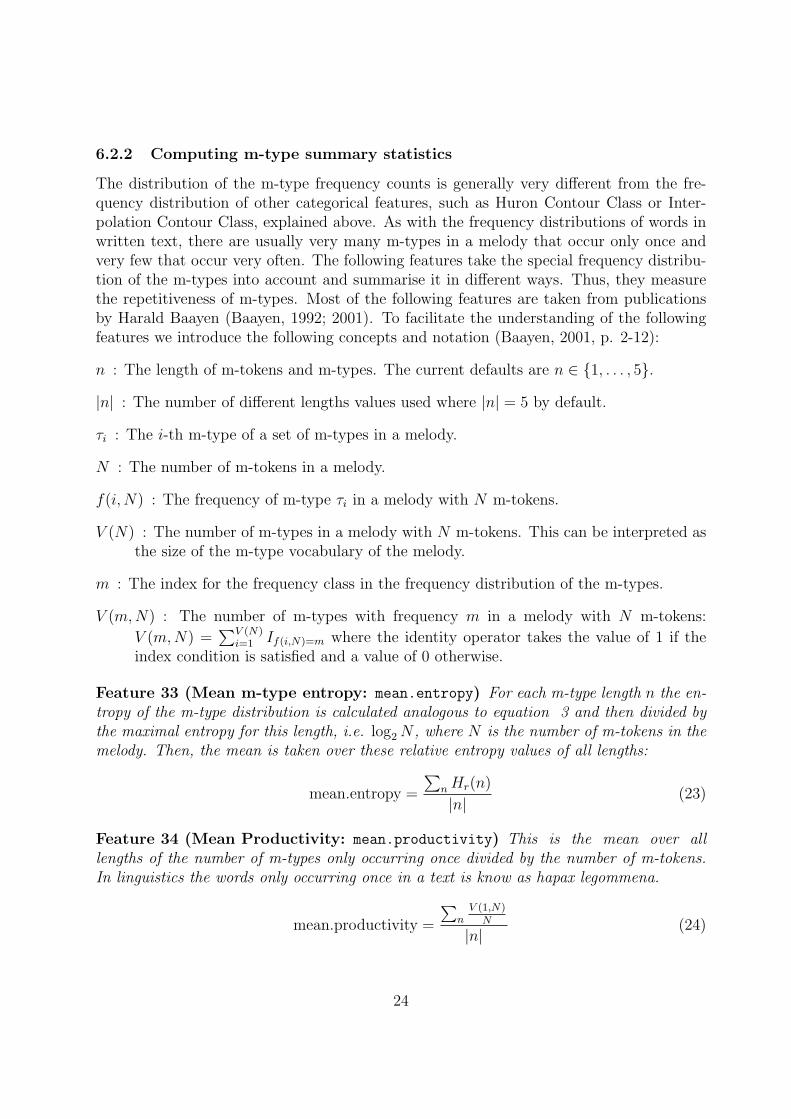
6.2.2 Computing m-type summary statistics

The distribution of the m-type frequency counts is generally very different from the fre-quency distribution of other categorical features, such as Huron Contour Class or Inter-polation Contour Class, explained above. As with the frequency distributions of words inwritten text, there are usually very many m-types in a melody that occur only once andvery few that occur very often. The following features take the special frequency distribu-tion of the m-types into account and summarise it in different ways. Thus, they measurethe repetitiveness of m-types. Most of the following features are taken from publicationsby Harald Baayen (Baayen, 1992; 2001). To facilitate the understanding of the followingfeatures we introduce the following concepts and notation (Baayen, 2001, p. 2-12):

n : The length of m-tokens and m-types. The current defaults are n ∈ {1, . . . , 5}.

|n| : The number of different lengths values used where |n| = 5 by default.

τi : The i-th m-type of a set of m-types in a melody.

N : The number of m-tokens in a melody.

f(i, N) : The frequency of m-type τi in a melody with N m-tokens.

V (N) : The number of m-types in a melody with N m-tokens. This can be interpreted asthe size of the m-type vocabulary of the melody.

m : The index for the frequency class in the frequency distribution of the m-types.

V (m,N) : The number of m-types with frequency m in a melody with N m-tokens:

V (m,N) =∑V (N)

i=1 If(i,N)=m where the identity operator takes the value of 1 if theindex condition is satisfied and a value of 0 otherwise.

Feature 33 (Mean m-type entropy: mean.entropy) For each m-type length n the en-tropy of the m-type distribution is calculated analogous to equation 3 and then divided bythe maximal entropy for this length, i.e. log2N , where N is the number of m-tokens in themelody. Then, the mean is taken over these relative entropy values of all lengths:

mean.entropy =

∑nHr(n)

|n|(23)

Feature 34 (Mean Productivity: mean.productivity) This is the mean over alllengths of the number of m-types only occurring once divided by the number of m-tokens.In linguistics the words only occurring once in a text is know as hapax legommena.

mean.productivity =

∑nV (1,N)N

|n|(24)

24

Feature 35 (Yules’s k: mean.Yules.K) Yule proposed this feature in 1944 to measurethe rate which words are repeated in a text, see (Baayen, 2001, p. 25) for a discussion.

mean.Yules.K =1

|n|· 1000 · (

∑mm

2V (m,N))−NN2

(25)

Feature 36 (Simpsons’s D: mean.Simpsons.D) Simpson’s D is was conceived to mea-sure word repetition rate as well and is mathematically closely related to Yule’s k.

mean.Simpsons.D =1

|n|∑m

V (m,N) · mN· m− 1

N − 1(26)

Feature 37 (Sichel’s S: mean.Sichels.S) Sichel’s S is based on the empirical observa-tion that the proportion of dis legommena (the words that occur twice) with respect to thevocabulary size is often constant throughout a text. It is defined by:

mean.Sichels.S =1

|n|· V (2, N)

V (N)(27)

Feature 38 (Honore’s H: mean.Honores.H) This feature is based on the assumptionthat the proportion of m-types only occurring once (hapax legommena) is a logarithmicfunction of the number of m-tokens.

mean.Honores.H =1

|n|· 100 · logN

1.01− V (1,N)V (N)

(28)

7 Corpus-based Feature Statistics

There is substantial support - both theoretical and empirical - in the literature for theassertion that the frequencies with which feature values occur in a domain might be animportant determinant for how these features are cognitively processed.13 This sectiondescribes how the two main functions derive frequency values from melody features withrespect to corpus of melodic phrases.

7.1 Frequencies of Summary Features

For the features summarising the content of a melody or a melodic phrase 6.1 obtainingfrequency-related information for a particular melody and from a corpus is straightforward.We replace the feature values with the relative frequency or frequency density with whichthey occur in the corpus. We, thus, eliminate the specific information about how large the

13 Essentially, David Huron’s latest book (2006) is all about how statistical properties of music influencemusic cognition. Looking outside music research and, for example, turning to psychological memoryresearch, the importance of word frequency for verbal memory and and cognitive text processing has beenfound in a large number of experiments.

25

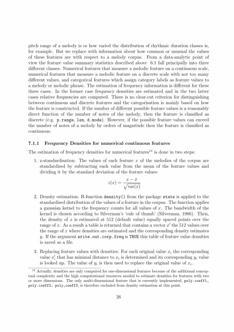
pitch range of a melody is or how varied the distribution of rhythmic duration classes is,for example. But we replace with information about how common or unusual the valuesof these features are with respect to a melody corpus. From a data-analytic point ofview the feature value summary statistics described above 6.1 fall principally into threedifferent classes: Numerical features that measure a melodic feature on a continuous scale,numerical features that measure a melodic feature on a discrete scale with not too manydifferent values, and categorical features which assign category labels as feature values toa melody or melodic phrase. The estimation of frequency information is different for thesethree cases. In the former case frequency densities are estimated and in the two lattercases relative frequencies are computed. There is no clear-cut criterion for distinguishingbetween continuous and discrete features and the categorisation is mainly based on howthe feature is constructed. If the number of different possible feature values is a reasonablydirect function of the number of notes of the melody, then the feature is classified asdiscrete (e.g. p.range, len, d.mode). However, if the possible feature values can exceedthe number of notes of a melody by orders of magnitude then the feature is classified ascontinuous.

7.1.1 Frequency Densities for numerical continuous features

The estimation of frequency densities for numerical features14 is done in two steps:

1. z-standardisation: The values of each feature x of the melodies of the corpus arestandardised by subtracting each value from the mean of the feature values anddividing it by the standard deviation of the feature values:

z(x) =x− x√var(x)

2. Density estimation: R-function density() from the package stats is applied to thestandardised distribution of the values of a feature in the corpus. The function appliesa gaussian kernel to the frequency counts for all values of x. The bandwidth of thekernel is chosen according to Silverman’s ‘rule of thumb’ (Silverman, 1986). Then,the density of x is estimated at 512 (default value) equally spaced points over therange of x. As a result a table is returned that contains a vector x′ the 512 values overthe range of x where densities are estimated and the corresponding density estimatesy. If the argument write.out.corp.freq is TRUE this table of feature value densitiesis saved as a file.

3. Replacing feature values with densities: For each original value xi the correspondingvalue x′i that has minimal distance to xi is determined and its corresponding yi valueis looked up. The value of yi is then used to replace the original value of xi.

14 Actually, densities are only computed for one-dimensional features because of the additional concep-tual complexity and the high computational resources needed to estimate densities for features with twoor more dimensions. The only multi-dimensional feature that is currently implemented, poly.coeff1,poly.coeff2, poly,coeff3, is therefore excluded from density estimation at this point.

26

As a result a table is returned where all values xi are replaced by values yi. The setof continuous numerical features is p.entropy, p.std, i.abs.mean, i.abs.std,

i.entropy, d.range, d.median, d.entropy, d.eq.trans, d.half.trans,

d.dotted.trans, glob.duration, note.dens, tonalness, tonal.clarity,

tonal.spike, int.cont.grad.mean, int.cont.grad.std, step.cont.glob.var,

step.cont.glob.dir, step.cont.loc.var.

7.1.2 Relative frequencies for categorical features

The computation of relative frequencies for categorical features is done simply by dividingthe number of counts in each category by the sum of counts of all categories (i.e. thenumber of melodies or melodic phrases).

1. Relative frequency computation:

f(xi) =count(xi)∑i count(xi)

As a result a table is returned that contains the categorical feature values and theirrelative frequencies. If the argument write.out.corp.freq is TRUE this table ofrelative feature value frequencies value is saved as a file together with the table ofdensities of numerical features.

2. Replacing feature values with relative frequencies: Each categorical value of x isreplaced by its relative frequency.

As a result a table is returned where all category labels xi are replaced by their relativefrequencies yi. The set of categorical features is mode, h.contour, int.contour.class.

7.1.3 Relative frequencies for numerical discrete features

The computation of relative frequencies for discrete features is based a mixture betweenthe procedure for categorical and continuous features.

1. Relative frequency computation:

f(xi) =count(xi)∑i count(xi)

As a result a table is returned that contains the numerical feature values and theirrelative frequencies.

2. Replacing feature values with densities: For each original value xi the correspondingvalue x′i that has minimal distance to xi. The value of yi is then used to replaced xi.

As a result a table is returned where all numerical values xi are replaced by their relativefrequencies yi. The set of discrete numerical features is p.range, i.abs.range, i.mode,

d.mode, len, int.cont.glob.dir, int.cont.dir.change.

27

7.2 Features derived from m-type distributions in melody andcorpus

The distribution of the summary features and the m-types are fundamentally different.While summary features are generally assumed to be distributed according to a Gaussiandistribution (or a mixture of several Gaussians), m-types are assumed to be distributedaccording to a powerlaw, very similar to word frequency distributions in written texts.Deriving information from these two kinds of distribution is therefore an inherently differentprocedure. There are several ways in which the distributions of m-types in a melody withrespect to a corpus can be condensed into single-value features.

7.2.1 Comparisons between m-type distributions from melody and corpus

A very straightforward way to determine whether m-types are used in an unusual way in amelody is to compare their frequency of occurrence in the melody with their frequency ofoccurrence in the corpus. Similarity measures such as correlations, differencing, and vectormultiplication are used for comparison. We denote the frequency count of m-type τ in amelody m by TFτ (derived from term frequency in information retrieval), and we use DFτ(from Document Frequency) for the number of melodies in the corpus containing τ .

Feature 39 (Spearman corr. of term and doc. frequencies: mtcf.TFDF.spearman)For this feature the ranks of TFτ∈m and DFτ∈m are correlated using Spearman’s rankcorrelation. For ties in the values (frequency counts) in TF and DF the minimum rank isassigned to all ranks in the same set of ties. The value is range from −1 to 1.

Feature 40 (Kendall’s τ of term and document frequencies: mtcf.TFDF.kendall)This feature is similar to mtcf.TFDF.spearman but uses the well-known correlation methodknown as Kendall’s τ . For ties in the values (frequency counts) in TF and DF the mini-mum rank is assigned to all ranks in the same set of ties. The value is range from −1 to1.

Feature 41 (Mean dot product of term and doc. frequencies: mean.log.TFDF)The rationale behind this feature is to use the dot product to measure the similaritybetween the vector of the term frequencies and the vector of the document frequenciesfor all m-types τ contained in a melody. Assuming that m-type frequencies, like wordfrequencies in texts, are approximately distributed according to an exponential distribution,both vectors are first transformed logarithmically and then standardised:

TF′τi∈m =log2(TFτi∈m)∑i log2(TFτi∈m)

where the same transformations are applied to DFτ∈m. We then take the mean of thevector resulting from vector multiplication:

mtcf.mean.log.TFDF =TF′τ∈m ·DF′τ∈m|τ ∈ m|

(29)

28

Feature 42 (Normalised distance of term and doc. frequencies: norm.log.dist)The same logarithmic and standardisation transformations used for mean.log.TFDF areapplied as a first stage for this feature. Then, instead of multiplying the elements of bothvectors their difference is taken and averaged:

mtcf.norm.log.dist =

∑τi∈m |TF

′τi−DF ′τi |

|TFτ∈m|(30)

7.2.2 Features derived from m-type corpus frequencies

These features are the closest equivalent to word frequencies derived from a corpus inlinguistic or psycho-linguistic applications and are intended to reflect how common or rarethe m-types are that are found in an analysis melody.

Feature 43 (Maximum document frequency: mtcf.max.log.DF) This is simply thelogarithm of the m-type contained in the analysis that also occurs in a maximum numberof melodies in the corpus.

max.log.DF = log2(max(DFτ∈m)) (31)

Feature 44 (Minimum document frequency: mtcf.min.log.DF) Conversely tomtcf.max.log.DF this feature measures how rare m-type with the least occurrences in thecorpus is.

min.log.DF = log2(min(DFτ∈m)) (32)

Feature 45 (Mean document frequency: mtcf.mean.log.DF) This feature reflectshow common or rare the m-types contained in a melody are on average:

mean.log.DF =

∑DFτ∈m|DFτ∈m|

(33)

Feature 46 (Mean document frequency entropy: mtcf.mean.entropy) This fea-ture is very similar to mean.entropy, but instead of the frequencies of the m-types in theanalysis melody fc(τi) it uses the frequencies of the in the corpus, fC(τi). Just like formean.entropy, the entropy values are averaged over the various m-types lengths.

Feature 47 (Mean document frequency productivity: mtcf.mean.productivity)This feature is very similar to mean.productivity, but instead of the frequencies of them-types in the analysis melody fc(τi) it uses the frequencies of the in the corpus, fC(τi).Just like for mean.productivity, the productivity values are averaged over the variousm-types lengths.

Feature 48 (Mean document frequency Yule’s K: mtcf.mean.Yules.K) This fea-ture is very similar to mean.Yules.K, but instead of the frequencies of the m-types inthe analysis melody fc(τi) it uses the frequencies of the in the corpus, fC(τi). Just like formean.Yules.K, the K values are averaged over the various m-types lengths.

29

Feature 49 (Mean document frequency Simpson’s D: mtcf.mean.Simpsons.D)This feature is very similar to mean.Simpsons.D, but instead of the frequencies of them-types in the analysis melody fc(τi) it uses the frequencies of the in the corpus, fC(τi).Just like for mean.Simpsons.D, the D values are averaged over the various m-typeslengths.

Feature 50 (Mean document frequency Sichel’s S: mtcf.mean.Sichels.S) Thisfeature is very similar to mean.Sichels.S, but instead of the frequencies of the m-typesin the analysis melody fc(τi) it uses the frequencies of the in the corpus, fC(τi). Just likefor mean.Sichels.S, the S values are averaged over the various m-types lengths.

Feature 51 (Mean document frequency Honore’s H: mtcf.mean.Honores.H)This feature is very similar to mean.Honores.H, but instead of the frequencies of them-types in the analysis melody fc(τi) it uses the frequencies of the in the corpus, fC(τi).Just like for mean.Honores.H, the H values are averaged over the various m-types lengths.

7.2.3 Features derived from m-type melody frequencies and inverted m-typecorpus frequencies

A simple and very wide-spread scheme for weighting words in text retrieval is to multiplythe frequency with which a type or term occurs in a text with the inverse of the frequencywith which it occurs in a text corpus. Types that are rare in general but frequent in agiven document thus get a high weight. The analogue can be constructed for m-typesin melodies. With reference to text retrieval we shall use the hereIDFC(τ) to denote theinverse document frequency of the m-type τ in melody corpus C:

IDFC(τ) =|C|

|c ∈ C : τ ∈ c|With TFc(τ) we denote here what we called above f(τ,N), i.e. the frequency of m-typeτ in melody c(with N tokens which is irrelevant here). The final TF-IDF weight for τ istderived by multiplication of term and inverted document frequency, TFc(τ)× IDFC(τ).

Feature 52 (Mean TF-IDF entropy: mtcf.TFIDF.m.entropy) This feature is verysimilar to mean.entropy, but instead of the frequencies of the m-types in the analysismelody fc(τi) it uses the TF-IDF weights. Just like for mean.entropy, the entropy valuesare averaged over the various m-types lengths.

Feature 53 (Mean TF-IDF Yule’s K: mtcf.TFIDF.m.K) This feature is very similarto mean.Yules.K, but instead of the frequencies of the m-types in the analysis melodyfc(τi) it uses the TF-IDF weights. Just like for mean.Yules.K, the K values are averagedover the various m-types lengths.

Feature 54 (Mean TF-IDF Sichel’s S: mtcf.TFIDF.m.S) This feature is very similarto mean.Sichels.S, but instead of the frequencies of the m-types in the analysis melodyfc(τi) it uses the TF-IDF weights. Just like for mean.Sichels.S, the S values are averagedover the various m-types lengths.

30

7.2.4 Features derived from entropy-based weightings

In modern text retrieval and psycholinguistics a considerable amount of attention hasbeen given to weighting schemes that are based on word frequencies and should reflect theimportance, weight, or specificity of a word to a particular context (section or paragraph ofa written text). We use the weighting scheme suggested for use with the Latent SemanticAnalysis algorithm in Quesada (2007, p. 80-81). Similar to the TFDF-based featuresabove the entropy-based weighting consists of local weight and a global weight. The localweight of an m-type τ is the logarithm of its frequency in the analysis melody +1:

loc.w(τ) = log2(f(τ) + 1)

The global weight of an m-type is based on the ratio Pτ , i.e. the ratio of its its localfrequency in each melody c of the corpus to the overall frequency in the corpus C:

Pc(τ) =fc(τ)

fC(τ)

The global weight is then calculated as follows:

glob.w = 1 +

∑c∈C

Pc(τ) · log2(Pc(τ))

log2(|C|)

The final weight for m-type τ is then obtained by

glob.loc.w(τ) = loc.w(τ) · glob.w(τ)

Feature 55 (Mean global weight: mtcf.mean.g.weight) This is simply the mean ofthe global weights ( glob.w) of all m-types τ in the analysis melody.

Feature 56 (Standard deviation of global weights: mtcf.std.g.weight)Accordingly, mtcf.std.g.weight is an indicator of the variability of the global weightsthe m-types τ in the analysis melody.

Feature 57 (Mean global-local weight: mtcf.mean.gl.weight) This is simply themean of the combined global-local weights ( glob.loc.w) of all m-types τ in the analysismelody.

Feature 58 (Standard deviation of global-local weights: mtcf.std.gl.weight)Accordingly, mtcf.std.gl.weight is an indicator of the variability of the combinedglobal-local weights ( glob.loc.w) of all m-types τ in the analysis melody.

31

8 Similarity computation based on features and fea-

ture distributions

The function feature.similarity() offers several ways to compute the similarity be-tween melodies based on summary features as computed by compute.features() andtheir frequency distributions as computed by corpus.based.feature.frequencies().15

The computation of similarities is carried out in two steps:

1. Compute features for all input melodies by calling the function compute.features().The value of the argument use.segmentation is passed on to compute.features()

and the function is always called with output="melody.wise".

2. Similarities between melodies are computed based on their values for each feature andaccording to one of three different methods (see below). If argument average=FALSE,a list of separate matrices, one for each feature, is outputted, otherwise the outputlist contains only 1 matrix where similarity values are averaged over the featuresspecified.

8.1 Methods for computing similarities from features

Three different methods can be used to compute similarities from features. They all outputsimilarity values between 0 (minimal similarity) and 1 (maximal similarity / identity) forevery pair of melodies. The similarities computed here are currently always symmetric,meaning that σ(mi,mj) = σ(mj,mi), i.e. the order in which two melodies mi and mj arecompared does not matter.16

8.1.1 Euclidean Distance / Similarity

Euclidean distance is a well-known distance measure and is only suitable for determiningthe distance between melodies mi and mj on the basis of numerical features ki. It is definedas

deucl(mi,mj) =

√∑K

(xik − xjk)2

where xik is the value of melody mi on feature k and xjk is the value of melody mj onfeature k. This distance value is then divided by the number of features K and in orderto arrive at a similarity value from the interval [0, 1] an exponential transform is used:

σeucl(mi,mj) = e−deucl(mi,mj)

K ∈ [0, 1]

15 While similarity computations based on m-types have already been applied quite successfully to real-world problems (see Mullensiefen and Pendzich, 2009), feature.similarity() doesn‘t currently carryout similarity computations based on m-types or m-type features.

16 Asymmetric measures that performed well in a previous applications (Mullensiefen and Pendzich,2009) are to be integrated at some later stage.

32

If the argument eucl.stand is TRUE, then all feature values xi,k are z-standardised by

z(xi,k) =xi,k − xkvar(xk)

before computing the euclidean distance. The standardisation is recommended when fea-tures with different value ranges are combined into one similarity measure.

8.1.2 Similarity based on Gower’s coefficient

Gower’s general coefficient of similarity (Gower, 1971) has become a standard way ofcombining similarity measurements from variables of different measurement scales (binary(dichotomous), categorical (qualitative), and numerical (quantitative) variables). For cat-egorical variables Gower’s coefficient assigns a value of 1 when both objects have are fromthe same class and 0 if they are from different classes. For a numerical variable k Gowerdefines the similarity between objects (melodies) mi and mj by

σGower,k(mi,mj) = 1− |xi − xj|Rk

In contrast to the euclidean distance, the standardisation of the distance is done here bydividing by the range Rk of feature k (and not by its variance). Similarity values are thenaveraged over the K features specified. Details of this similarity coefficient can be foundin Gower (1971). Since Gower’s coefficient always standardises distance/similarity valuesby the range of the feature values, it gives misleading results when only few melodies areto be compared. In the case of just two input melodies their similarity is necessarily 0because the distance of their values on any (numerical) feature equals the range of thatfeature variable. It is therefore recommended to use Gower similarity only with larger setsof melodies as input.

8.1.3 Corpus-based similarity

This is a novel approach to similarity computation that makes use of the musical back-ground information as is manifest in the frequency distribution of numerical features ina corpus. The core idea is to replace the actual difference between the feature values fortwo melodies by the difference in the cumulative sums of melodies from a corpus at thesefeature values. Thus, a difference of 0.2 arising from feature values xi = 0.6 and xj = 0.4can mean something else than a difference of 0.2 obtained from xi = 0.9 and xj = 0.7 if thebulk of melodies from a corpus scores values between, say 0.3 and 0.7 on that feature. Inthat case, the difference between 0.9 and 0.7 seems to indicate a higher similarity becausehigh feature values happen less frequently than feature values broadly around 0.5. Thesimilarity between two melodies mi and mj on a numerical feature k in the context of acorpus C is thus defined as

σcorpus,k,C(mi,mj) = |l=xi∑l=1

fC(xl)−l=xj∑l=1

fC(xl)|

33

where l is the index of the discrete frequency distribution from corpus C and∑l=xi

l=1 fC(xl) is the cumulative frequency count of the distribution between the first binl = 1 and the bin at feature value xi.

For categorical features corpus-based similarity equals Gower similarity, giving 1 tomelodies having the same class and 0 having different classes. If average=TRUE similarityvalues from different features are combined by a weighted average. The weighting is doneaccording to the entropy of the frequency distribution of each feature. Features with higherentropy are given a higher weight.

Acknowledgements

This research was funded by EPSRC grant EP/D0388551. The author likes to thank KlausFrieler, Andrea Halpern, Ruben Hillewaere, and David Lewis for very valuable commentson earlier drafts of this report and on the Fantastic code itself.

References

Arom, S. (1991). African Polyphony and Polyrhythm. Musical Structure and Methodology.Cambridge University Press, Cambridge.

Baayen, H. (1992). Quantitative aspects of morphological productivity. In Booij, G. andvan Marle, J., editors, Yearbook of Morphology 1991. Theme: Morphological Classes,pages 109–150. Springer.

Baayen, H. (2001). Word Frequency Distributions. Kluwer Academic Publishers.

Bilmes, J. A. (1993). Timing is of the essence: Perceptual and computational techniques forrepresenting, learning, and reproducing expressive timing in percussive rhythm. Master’sthesis, School of Architecture and Planning, MIT, Boston [MA].

Dowling, W. J. (1972). Recognition of melodic transformations: Inversion, retrograde, andretrograde inversion. Perception & Psychophysics, 12(5):417–421.

Downie, J. S. (2003). Evaluating a simple approach to music information retrieval. Eval-uating a simple approach to music information retrieval. Conceiving melodic n-gramsas text. PhD thesis, Faculty of Information and Media Studies, University of WesternOntario, London (Ontario), Canada.

Eerola, T. and Toiviainen, P. (2004). Mir in matlab: The midi toolbox. In Proceedings ofthe 5th International Conference on Music Information Retrieval.

Frieler, K. (2005). Melody - csv file format (mcsv), technical documentation. unpublished.

Gower, J. C. (1971). A general coefficient of similarity and some of its properties. Biomet-rics, 27(4):857–871.

34

Hood, M. (1971). The Ethnomusicologist. McGraw-Hill, New York.

Huron, D. (1996). The melodic arch in western folksongs. Computing in Musicology,10:3–23.

Jesser, B. (1990). Interaktive Melodieanalyse: Methodik und Anwendung computergestutzterAnalyseverfahren in Musikethnologie und Volksliedforschung. Typologische Untersuchungder Balladensammlung des DVA. Peter Lang, Bern.

Juhasz, Z. (2000). A model of variation in the music of a hungarian ethnic group. Journalof New Music Research, 29(2):159–172.

Krumhansl, C. L. (1990). Cognitive Foundations of Musical Pitch. Oxford PsychologySeries 17. Oxford University Press, Oxford.

Krumhansl, C. L. and Kessler, E. (1982). Tracing the dynamic changes in perceived tonalorganization in a spatial representation of musical keys. Psychological Review, 89:334–368.

Kubik, G. (1998). Zum Verstehen afrikanischer Musik. Philipp Reclam junior, Leipzig.

Lomax, A. (1977). Cantometrics: An Approach to the Anthropology of Music. Universityof California, Berkley.

Mullensiefen, D. and Frieler, K. (2004). Cognitive adequacy in the measurement of melodicsimilarity: Algorithmic vs. human judgments. Computing in Musicology, 13:147–176.

Mullensiefen, D. and Frieler, K. (2006). The SIMILE algorithms documentation 0.3.

Mullensiefen, D. and Wiggins, G. A. (2009). Polynomial functions as a representation ofmelodic phrase contour. under review.

Pfleiderer, M. (2006). Rhythmus: Psychologische, theoretische und stilanalytische Aspektepopularer Musik. transcript, Bielefeld.

Quesada, J. (2007). Creating your own LSA spaces. In Landauer, T. K., McNamara, D. S.,Dennis, S., and Kintch, W., editors, Handbook of Latent Semantic Analysis, chapter 4,pages 71–85. Lawrence Erlbaum Associates.

Sadakata, M., Desain, P., and Honing, H. (2006). The bayesian way to relate rhythmperception and production. Music Perception, 23(3):269–288.

Sagrillo, D. (1999). Melodiegestalten im luxemburgischen Volkslied: Zur Anwendung com-putergestutzter Verfahren bei der Klassifikation von Volksliedabschnitten. Holos, Bonn.

Shannon, C. E. (1948). A mathematical theory of communication. Bell Systems TechnicalJournal, 27:379–423, 623–656.

35

Silverman, B. W. (1986). Density Estimation. Chapman and Hall, London.

Steinbeck, W. (1982). Struktur und Ahnlichkeit: Methoden automatisierter Melodieanalyse.Barenreiter, Kassel.

Temperley, D. (2001). The Cognition of Basic Musical Structures. MIT Press, Cambridge,MA.

Temperley, D. (2007). Music and Probability. MIT Press, Cambridge, MA.

Uitdenbogerd, A. L. (2002). Music Information Retrieval Rechnology. PhD thesis, RMITUniversity of Melbourne, Australia.

36

Index

d.dotted.trans, 16d.entropy, 15d.eq.trans, 16d.half.trans, 16d.median, 15d.mode, 15d.range, 15

glob.duration, 16

h.contour, 17

i.abs.mean, 14i.abs.range, 14i.abs.std, 15i.entropy, 15i.mode, 15int.cont.dir.changes, 19int.cont.glob.dir, 19int.cont.grad.mean, 19int.cont.grad.std, 19

len, 16

mean.entropy, 24mean.Honores.H, 25mean.log.TFDF, 28mean.productivity, 24mean.Sichels.S, 25mean.Simpsons.D, 25mean.Yules.K, 25mode, 22mtcf.max.log.DF, 29mtcf.mean.entropy, 29mtcf.mean.g.weight, 31mtcf.mean.gl.weight, 31mtcf.mean.Honores.H, 30mtcf.mean.log.DF, 29mtcf.mean.productivity, 29mtcf.mean.Sichels.S, 30mtcf.mean.Simpsons.D, 30

mtcf.mean.Yules.K, 29mtcf.min.log.DF, 29mtcf.std.g.weight, 31mtcf.std.gl.weight, 31mtcf.TFDF.kendall, 28mtcf.TFDF.spearman, 28mtcf.TFIDF.m.entropy, 30mtcf.TFIDF.m.K, 30mtcf.TFIDF.m.S, 30

norm.log.dist, 29note.dens, 17

p.entropy, 14p.range, 13p.std, 14ploy.coeff1, 21ploy.coeff2, 21ploy.coeff3, 21

step.cont.glob.dir, 18step.cont.glob.var, 18step.cont.loc.var, 18

tonal.clarity, 22tonal.spike, 22tonalness, 22

37