False Discovery Rates and Copy Number Variation

Bradley Efron∗ Nancy Zhang†

Department of StatisticsStanford University

AbstractCopy number changes, the gains and losses of chromosome segments, are a common type

of genetic variation among healthy individuals as well as an important feature in tumorgenomes. Microarray technology enables us to simultaneously measure, with moderateaccuracy, copy number variation at more than a million chromosome locations and forhundreds of subjects. This leads to massive data sets and complicated inference problemsconcerning which locations for which subjects are genuinely variable. In this paper weconsider a relatively simple false discovery rate approach to cnv analysis. More carefulparametric change-point methods can then be focused on promising regions of the genome.

Key words and phrases: False discovery rate, multiple testing, grouped hypotheses, DNAcopy number

1 Introduction

Basic genetics says that we have two copies of each bit of chromosomal information. In fact,however, even healthy individuals show occasional variations, displaying stretches of the genomehaving more or less than two copies. Within the past decade, significant advances in microarraytechnology have enabled the genome-wide fine scale measurement of DNA copy number in highthroughput fashion; see Bignell et al. (2004); Peiffer et al. (2006); Pinkel et al. (1998); Pollacket al. (1999); Snijders et al. (2001). This has led to large-scale studies investigating the role ofDNA copy number changes in human disease and phenotypic variation. The studies fall intotwo main categories: changes in DNA copy number can occur as a form of inherited geneticpolymorphism in normal human DNA. They can also accompany somatic mutation, as oftenobserved in cancerous tumors. Inherited copy number changes in normal samples have beencalled copy number variants (cnv), while those that occur in tumors have been referred to ascopy number aberrations (cna), to distinguish the fact that they are “aberrant” forms whichdo not occur as population-wide variation. This paper discusses a false discovery rate approachto the analysis of DNA copy number data.

The statistical properties of copy number data are quite different in the two cases. Innormal samples, the copy number variants, most of which are inherited, are usually short andspaced far apart, whereas in tumor samples, cnas can be quite long, sometimes spanning entirechromosomes. The false discovery rate (fdr) methodology developed in this paper applies toboth situations, but our examples will start by focusing on the first. We will discuss tumorsamples in more detail, with a data example, in Section 7.∗Research supported in part by NIH grant 8R01 EB002784 and by NSF grant DMS 0804324.†Research supported in part by NSF Grant DMS 0906394.

* *** * *** ****** * * * * *** *** ** * ** * *** * ***** ** * ** *** ** * * * * * ** * **** *** ** ******************* ** * * * ** * * * ** *** * * * * * * * * ****** * * * * * * * * * * * * ** * * ** ** * ** * ** *** * ** * ** * * ******************** ***** **** * * ** * * * * * * * *** ** ** * ** ** * * ** * *** * * * * *** * * * **** ******* *** ** * * * * * ** ** ** * * ** ** ** ***** * * ***** ** ** * ** **** ***** * **** *** ** * ** *** ** * * ** * ** * * ** ******** * * ****** * * ** ** * ** **** ********************************************************************** ***** * *** * * * * * * ** * * ** * *** * ***** *** ** *** * ** * ** ** * ** * ** * **** * ** * * * * *** * ** * * * * * ** ** * * * ** * * * * * * * * * * ** * * ** ** * * * ****** ** *** *** * * ***** * * * * **** *********************************************************** ** ** * *** ************ ** * *** * * * * * * * * * * * * * * * * * * *** ** * **** * * *** * ** ** * ** * * * * ******************************************* * * ** * * * **** * * ** ** * ** * ** ** ** * * *

0 1000 2000 3000 4000 5000

050

100

150

position number i −>

subj

ect n

umbe

r j −

>

45

1755

Interval

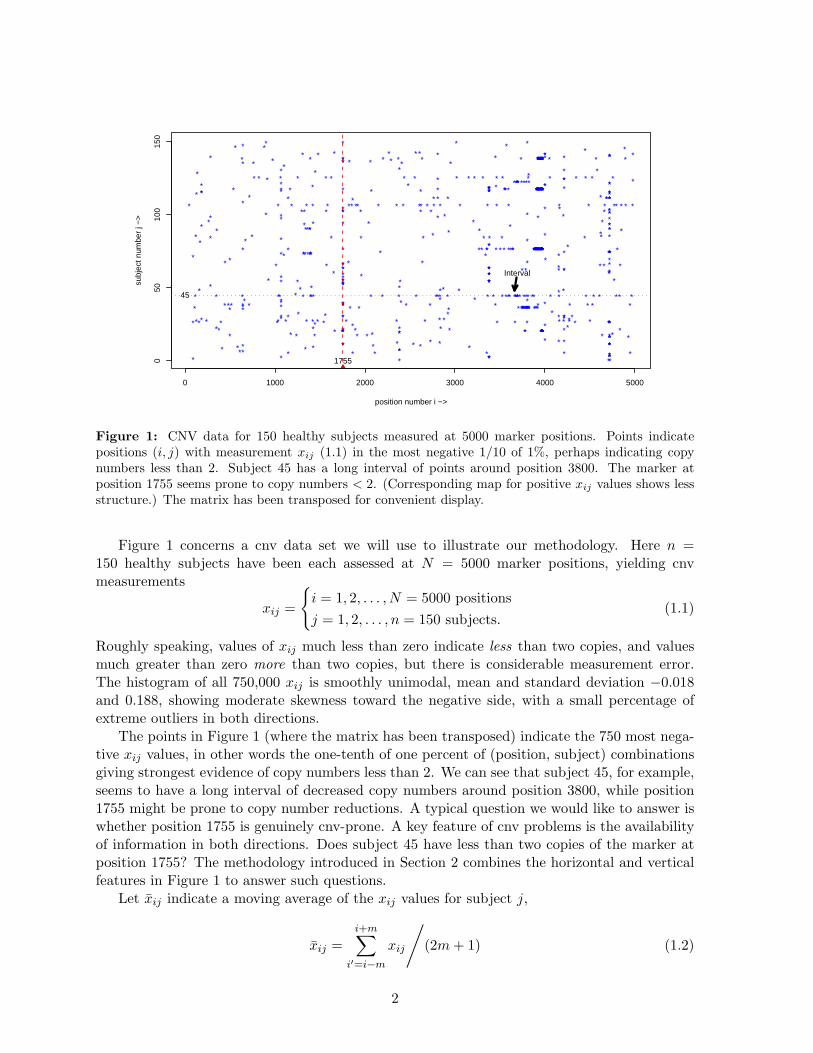
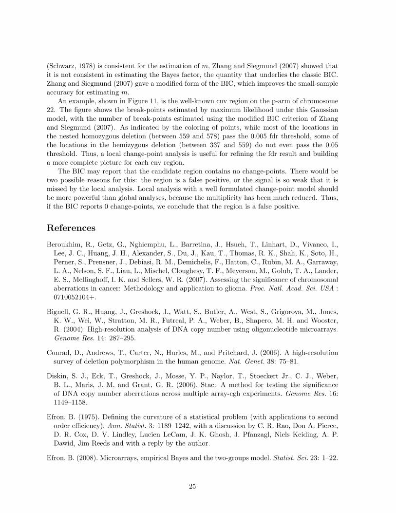
Figure 1: CNV data for 150 healthy subjects measured at 5000 marker positions. Points indicatepositions (i, j) with measurement xij (1.1) in the most negative 1/10 of 1%, perhaps indicating copynumbers less than 2. Subject 45 has a long interval of points around position 3800. The marker atposition 1755 seems prone to copy numbers < 2. (Corresponding map for positive xij values shows lessstructure.) The matrix has been transposed for convenient display.

Figure 1 concerns a cnv data set we will use to illustrate our methodology. Here n =150 healthy subjects have been each assessed at N = 5000 marker positions, yielding cnvmeasurements

xij =

{i = 1, 2, . . . , N = 5000 positionsj = 1, 2, . . . , n = 150 subjects.

(1.1)

Roughly speaking, values of xij much less than zero indicate less than two copies, and valuesmuch greater than zero more than two copies, but there is considerable measurement error.The histogram of all 750,000 xij is smoothly unimodal, mean and standard deviation −0.018and 0.188, showing moderate skewness toward the negative side, with a small percentage ofextreme outliers in both directions.

The points in Figure 1 (where the matrix has been transposed) indicate the 750 most nega-tive xij values, in other words the one-tenth of one percent of (position, subject) combinationsgiving strongest evidence of copy numbers less than 2. We can see that subject 45, for example,seems to have a long interval of decreased copy numbers around position 3800, while position1755 might be prone to copy number reductions. A typical question we would like to answer iswhether position 1755 is genuinely cnv-prone. A key feature of cnv problems is the availabilityof information in both directions. Does subject 45 have less than two copies of the marker atposition 1755? The methodology introduced in Section 2 combines the horizontal and verticalfeatures in Figure 1 to answer such questions.

Let xij indicate a moving average of the xij values for subject j,

xij =i+m∑

i′=i−mxij

/(2m+ 1) (1.2)

2

for some fixed value of m (with obvious modifications for i near 1 or N). Because cnv intervalstend to span a contiguous range of marker positions, xij will be less noisy than xij ; see Section 5for the specific calculation. It is also helpful to standardize the columns of the {xij} matrix,that is, each subject’s xij values, by defining

zij = (xij − aj)/bj (1.3)

where aj and bj are the median and robust standard deviation (one-half the distance betweenthe 16th and 84th percentiles) of {xij : i = 1, 2, . . . , N}. Most of our numerical examples will bebased on zij values (1.2), (1.3) with m = 5. The application of fdr methodology to the z-valuesrenders copy number variations far more visible; see Figure 3.

The paper develops as follows: an iterative algorithm is introduced in Section 2, in whicha local false discovery rate estimate (Efron, 2008) is first fit to the combined data, and thenmodified to take account of differing cnv probabilities at the various positions i. This gives anfdr estimate for each position and subject, as well as an estimate ki of the number of subjectscarrying a cnv at position i.

Section 3 and Section 4 develop hypothesis-testing and estimation methods based on the ki’s,aimed at answering the question of which, if any, of the positions are cnv-prone. The iterativealgorithm is examined more closely in Section 5 and Section 6, and connected to maximumlikelihood theory. Section Section 7 examines in more detail the problem of detecting cna-prone regions in tumors. Having located positions prone to copy number changes based on theki estimates, Section 7 then discusses local change-point methods intended to say which of thesubjects are the affected ones, the so-called “carriers.”

There are by now many different methods for single-sample analysis of DNA copy number.These methods process each sample (i.e., each column in the matrix (1.1)) separately, as ifthe method has never seen a similar sample before, and will never see another sample again.Reviews of single-sample methods are given in Lai et al. (2005), Willenbrock and Fridlyand(2005), and Zhang (2010). For both single-sample analysis and the simultaneous processing ofmultiple samples, global change-point tests, scanning over the entire range of positions, haveplayed a central role in the statistical cnv lierature (Olshen et al., 2004; Siegmund, Yakir andZhang, 2010; Zhang et al., 2010). The literature leans heavily on Gaussian process theory, andwithin that realm produces impressively precise testing algorithms. Wang et al. (2005) proposean fdr approach, closer to the methods proposed here.

The identification of cnv-prone regions across a cohort of tumor samples has been a problemof increased scientific interest. Most published methods (Beroukhim et al., 2007; Diskin et al.,2006; Guttman et al., 2007; Newton et al., 1998; Newton and Lee, 2000; Rouveirol et al., 2006;Taylor et al., 2008) take a post-segmentation approach: each sample is first segmented individ-ually, which reduces them to piece-wise constant sequences indicating regions of amplification,deletion, or normal copy number. Then the samples are aligned, and a statistical model (New-ton et al., 1998; Newton and Lee, 2000) or permutation-based approach (Diskin et al., 2006)is used to identify regions of highly recurrent aberration. These post-segmentation approachesrely on the vagaries of the underlying segmentation model. After segmentation, how evidencefor gains and losses should be combined across samples is still much debated. Existing strategiesrange from counting the number of carriers, without weighting by the strength of evidence ofeach carrier (e.g., Diskin et al. (2006)), to the “G-score” (Beroukhim et al., 2007), defined asthe number of carriers times the average amplitude of the signal among carriers. The fdr-basedapproach that we describe arises from a natural likelihood model, is simple and computationally

3

fast, and yields biologically meaningful results.

2 False Discovery Rate Methods

Forgetting about cnv structure for a moment, suppose we have M null hypotheses H01, H02, . . . ,H0M to test, based on possibly correlated test statistics z1, z2, . . . , zM . False discovery ratemethods can be motivated by the Bayesian two-groups model discussed at length in Efron(2008), in which each case is either null or non-null with prior probability π0 or π1 = 1 − π0,and with the z values having density either f0(z) or f1(z),

π0 = Pr{null} f0(z) = density if nullπ1 = Pr{non-null} f1(z) = density if non-null.

(2.1)

Bayes rule shows that the posterior probability of “null” given z, the local false discovery rate,is

fdr(z) = Pr{null|z} = π0f0(z)/f(z) (2.2)

where f(z) is the mixture density

f(z) = π0f0(z) + π1f1(z). (2.3)

An empirical Bayes approach to multiple testing uses the entire vector z = (z1, z2, . . . , zM )to estimate π0, f0(z), f(z), and then fdr(z),

fdr(z) = π0f0(z)/f(z), (2.4)

rejecting the mth null hypothesis H0m if fdr(zm) is small, perhaps for fdr(zm) ≤ 0.1 or ≤ 0.01.(Replacing densities f0 and f1 with their cumulative distribution functions gets us back, almost,to Benjamini and Hochberg’s 1995 false discovery rate control algorithm, but here it will bemore convenient to deal directly with the densities.)

Figure 2 shows fdr(z) based on the combined data for all M = 750, 000 z values zij (1.3),computed using the locfdr algorithm, Efron (2008); locfdr assumes that f0(z) is normal, areasonable assumption here looking at the central portion of the {zij} histogram, which theaveraging in (1.2) renders quite Gaussian. The numerator estimates in (2.4) were

π0 = 0.954, f0 ∼ N (0.04, 0.932), (2.5)

obtained using the “central matching” (geometric) method. Taken literally, this implies 4.6%of the (i, j) pairs represent cnv locations,

π1 = 0.046. (2.6)

As discussed in Efron (2008), we can expect a majority of such pairs to have disappointinglylarge values of fdr(zij). Here only 1.5% of the 750,000 have fdr(zij) ≤ 0.1, those with zij ≤ −3.30or ≥ 3.56. However, we can improve power by adapting the fdr methodology to the two-waystructure of cnv data.

Let Ci be the class of pairs (i, j) corresponding to position i,

Ci = {(i, j) : j = 1, 2, . . . , n} (2.7)

4

−6 −4 −2 0 2 4 6

0.0

0.2

0.4

0.6

0.8

1.0

z values

fdrh

at(z

)

● ●

* *

−3.30 3.56

Figure 2: Estimated local false discovery rate fdr(z) based on all 750,000 values zij (1.3) for the cnvdata; fdr(z) is ≤ 0.1 for z ≤ −3.30 and z ≥ 3.56, respectively 1.2% and 0.3% of the 750,000 cases.Computed from program locfdr, Efron (2008).

so the corresponding z values zij are all those obtained at position i. We now have N classesC1, C2, . . . , CN , one for each position, and can imagine fitting a separate two-groups model (2.1)for each class, yielding separate false discovery rate functions fdri(z). The trouble is that, unlessn is very large, a direct approach as in Figure 2 will produce inaccurate estimates fdri(z).

A compromise between using the combined estimate fdr(z) or completely separate estimatesfdri(z) goes as follows: we assume that the null and non-null densities f0 and f1 in (2.1) applyunchanged to each class, but that the null and non-null prior probabilities may differ, say

πi0 = Pr{null|Ci} and πi1 = 1− πi0 = Pr{non-null|Ci}. (2.8)

So a cnv-prone position would be one having a larger value of πi1 than the combined value π1.Using fdri(z) = πi0f0(z)/f(i)(z), with f(i)(z) the mixture density applying to Ci,

f(i)(z) = πi0f0(z) + πi1f1(z), (2.9)

comparison with (2.2) gives

fdri(z) = fdr(z)/[1 + tdr(z) ·Ri] (2.10)

where tdr(z) is the true discovery rate

tdr(z) = 1− fdr(z) = Pr{non-null|z} (2.11)

andRi =

πi1/π1

πi0/π0− 1. (2.12)

An equivalent form istdri(z) = tdr(z)/[1 + fdr(z) · Si] (2.13)

5

now where tdri(z) = 1− fdri(z) is the true discovery rate Pr{non-null|z, Ci} applying to Ci, and

Si =πi0/π0

πi1/π1− 1. (2.14)

Section 6 discusses (2.10) and (2.13) in more detail.None of this seems like a step forward since (2.10) and (2.13) both require knowledge of

πi1, the non-null proportion in Ci. There is, however, a simple iterative solution. Given apreliminary estimate tdri(z) of tdri(z), perhaps tdr(z) from the combined analysis,

ki =∑j∈Ci

tdri(zij) =n∑j=1

tdri(zij) (2.15)

is the obvious estimate of ki, the number of non-null cases in Ci, since tdri(zij) estimates theprobability that case (i, j) is non-null.

This yields

πi1 = ki/n =

n∑j=1

tdri(zij)

/n (2.16)

as an estimate of πi1, and

Si =(1− πi1)

/π0

πi1/π1

− 1 (2.17)

for (2.14) (with π0 and π1 obtained from the combined analysis that gave fdr and tdr, as in(2.6)). We can now update (2.13) to

tdri(zij) = tdr(zij)/[

1 + fdr(zij)Si], (2.18)

recompute (2.15), etc. The numerical results that follow stopped after five iterations of (2.15)–(2.18), close to the final convergence values; see Section 6. Other examples, involving fewersubjects, required more iterations to reach convergence, though the increase did not noticeablyaffect subsequent inferences.

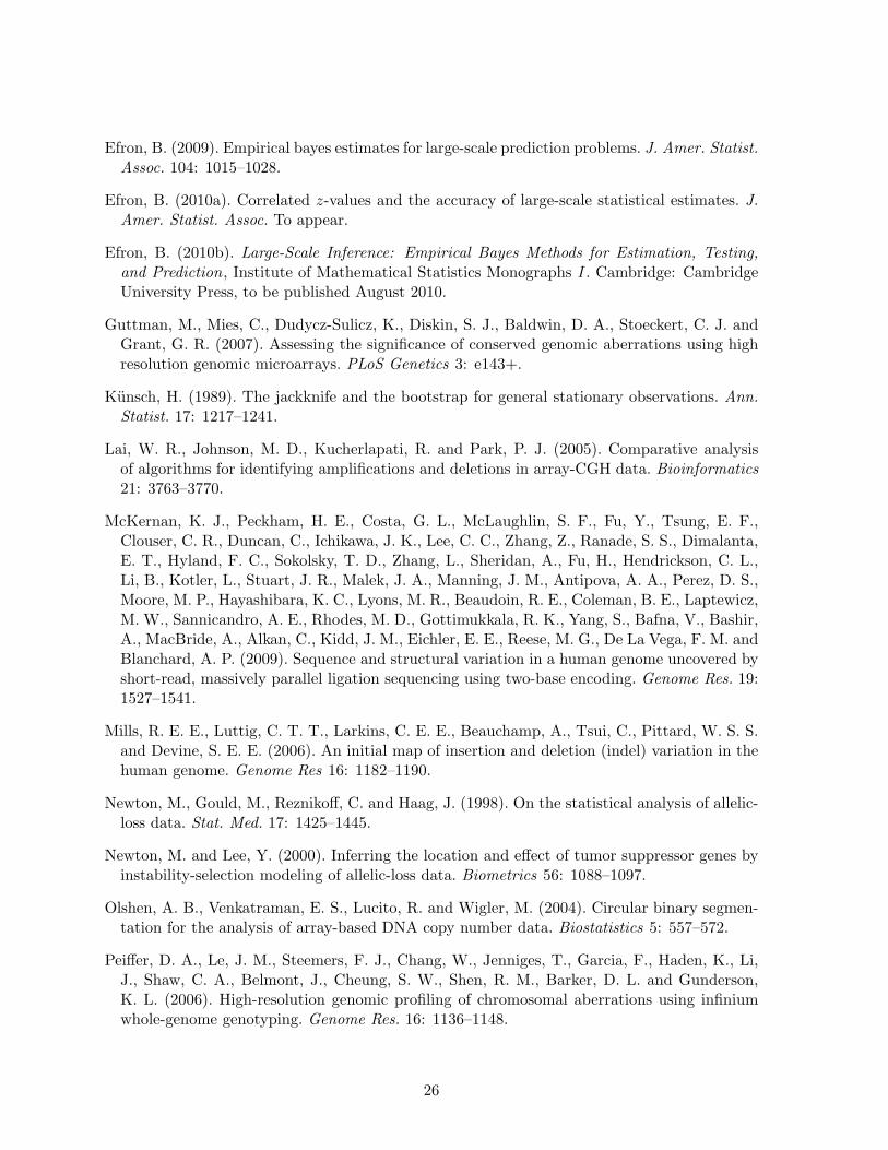
Figure 3 displays the results. The top panel shows those pairs (i, j) having tdri(zij) ≥ 0.99,or equivalently fdri(zij) ≤ 0.01. A very long cnv region is centered around i = 3800, withshorter but still prominent regions near 1, 1100, 1300, 3000, and 4700. Position i = 1755 is lessimpressive, but does show some non-null cases. The bottom panel graphs ki as a function ofposition i, with k1755 = 39.1 showing as a small isolated spike. Is this a “significant” result?The next two sections consider testing and estimation questions for the ki values.

3 Hypothesis Tests for Position-Wise Copy Number Variation

Having obtained estimates ki, i = 1, 2, . . . , N , for the number of non-null cnv subjects at markerposition i, we wish to decide which, if any, of the positions are unusually prone to copy numbervariation. For example, k1755 equals 39.1, compared to the average k = 8.13 in Figure 3, whichmight suggest excess variation at position 1755, an hypothesis we would like to test.

An easy permutation test proceeds as follows: let zj be the jth column of the Z matrix{zij} (1.3), and z∗j the same vector except shifted left I units (with wraparound),

z∗j = (zI+1,j , zI+2,j , . . . , zN,j , z1j , z2j , . . . , zIj)′. (3.1)

6

−−−−−−−−−−−−−−−−−−−−−−−−−−−−−−−−−−−−−−−−−−−−−−−−−−−−−−−−−−−−−−−−−−−−−−−−−−−−−−−−−−−−−−−− −−−−−−−−−− −− −−−−−−−−−−−−−− −− −−−−−−−−−−−−−−−−−−−−−−−−−−−−−−−−−−−− −−−−−−−−−−−−−−−−−−−−−−−−−−−−−−−−−−−−−−−−− −−−−−−−−−−− −−−−−−−−−− −−−−−−−−−− −−−−−−−−−−−−−−−−−−−−−−−−−−−−−−−−−−−−−−−−−−−− −−−−−− −−−−−−−−− −−−−−− −−−−−−−−−−−−−−−−−−−−−−−−−−−−−−−−−−−−−−−−−−−−−−− −−− −−−−−−− −−−− −−−−−−−−−−−−−−−−−−−−−−−−−−−−−−−−−−−−−−−−−−−−−−−−−−−−−−−−−−−−−−−−−−−−−− −−−−−−−−−−−−−−−−−−−−−−−−−−−−−−−−−−−−−−−−−−−−−−−−−−−−− −−−−−−− −−−−−−−−−−−−−−−−−−−−−−−−−−−−−−−−−−−−−−−−−−−−−−−−−−−−−−−−−−−−−−−−−−−−−−−−−−−−−−−−−−−−−−−−−−−−−−−−−−−−−−−−−−−−−−−−−−−−−−−−−−−−−−−−−−−−−−−−−−−−−−−−−−−−−−−−−−−−−−−−−−−−−−−−−−−−−−−−−−−−−−−−−−−−−−−−−−−−−−−−−−−−−−− −−−−−−−−−−−−−−−−−−−−−−−−−−− −−−− −−−−−−−−−−−−−−−−−−−−−−−−−−−−−−−−−−−−−−−− −−−−−−−−−−−−−−−−−−−−−−−−−−−−−−−−−−−−−−−−−−−−−− −−−−−−−−−−−−−−−−−−−−−−−−−−−−−−−−−−−−−−−−−−−−−−−−−−−−−−−−−−−−−−−−−−−−−−−−−−−−−−−−−− −−−−−−−− −−−−−−−−−−−−−−−− −−−−−−−−−−−−−−−−−−−−−−−−−−−−−−−−−−−−−−−−−−−−−−−−−−−−−−−−−−−−−−−−−−−−−−−−−−−−−−−−−−−−−−−−−−−−− −−−−−−−−−−−−−−−−−−−−−−−−−−−−−−−−−−−−−−−−−−−−−−− −−−−−−−−−−−−−−−−−−−−−−−−−−−−−−−−−−−−−−−−−−−−−−−−−−−−−−−−−−−−−−−−−−−−−−−−−−−−−−−−−−−−−−−−−−−−−−−−−−−−−−−−−−−−−−−−−−−−−−−−−−−−−−−−−−−−−−−−−−−−−−−−−−−−−−−−−−−−−−−−−−−−−−−−−−−−−−−−−−−−−−−−−−−−−−−−−−−−−−−−−−−−−−−−−−−−−−−−−−−−−−−−−−−−−−−−−−−− −−−−−−−−−− −−−−−−−−−−−−− −−−−−− −−−−−−−−−−−−−− −−−−− −− −−−−−−−−−−−−−− −−−−−−−−−−− −−−−−−− −−−−−−−−−−−−−−−−−−−−−−−−−−− −−−−−−−−−−− −−−−−−−−−− −−−−−−−−−−−−−−−−−−−−−−−−−−−−−−−− −−−−−−−−−−−−− −−−−−−−−− −−−−−−−−−− −−− −−−−− −−− −−−−−−−−−−−−−−−−−−−−−−−−−−−−−−−−−−−−−−−−−−−−−−−−−−−−−−−−−−−−−−−−−−−−− −−−−−−−−−−−−−−−−−−−−−−−−−−−−−−−−−−−−−−−−−−−−−−−−−−−−−−−−−−−−−−−−−−−−−−−−−−−−−−−−−−−−−−−−−−−−−−−−−−−−−−−−−−−−−−−−−−−−−−−−−−−−−−−−−−−−−−−−−−−−−−−−−−−−−−−−−−−−−−−−−−−−−−−−−−−−−−−−−−−−−−−−−−−−−−−−−−−−−−−−−−−−−−−−−−−−−−−−−−−−−−−−−−−−−−−−−−−−−−−−−−−−−−−−−−−−−−−−−−−−−−−−−−−−−−−−−−−−−−−−−−−−−−−−−−−−−−−−−−−−−−−−−−−−−−−−−−−−−−−−−−− −−−− −−− −−−−−−−−−−−−−−−−−−−−−−−−−−−−−−−−−−−−−−−−−−−−−−−−−−−−−−−−−−−−−−−−−−−−−−−−−−−−−−−−−−−−−−−−−−−−−−−−−−−−−−−−−−−−−−−−−−−−−−−−−−−−−−−−−−−−−−−−−−−−−−−−−−−−−−−−−−−−−−−−−−−−−−−−−−− −−−−−−−− −−−−−−−− −−−−−−−−−−− −−−−−−−−−− −−−−−−−−−−−−−−−−−−−−−−−−−−− −−−−−−−−−− −−−−− −−−−−− −−−−−−−−−−−−−−−−−−−−−−−−−−−−−−− −−−−−−−−−−−−−−−−−−−−−−−−−−−−−−−−−−−−−−−−−−−−−−−−−−−−−−−−−−−−−−−−−−−−−−−−−−−−−−−−−−−−−−−−−−−−−−−−−−−−−−−−−−−−−−−−−−−−−−−−−−−−−−−−−−−−−−−−−−−−−−−−−−−−−−−−−−−−−−−−−−−−−−−−−−−−−−−−−−−−−−−−−−−−−−−−−−−−−−−−−−−−−−−−−−−−−−−−−−−−−−−−−−−−−−−−−−−−−−−−−−−−− −−−−−−−−−−− −−−−−−−−−−− −−−−−−−−−−−−−−−−−−−−−−−−−−−−−−−−−−−−−−−−−−−−−−−−−−−−−−−−−−−−−−−−−−−−−−−−−− −−−−−−−−−−−−−−−−−−−−− −−−−−−−−−−−−−−−−−−−−−−−− −−−−−−−−−−−−−−−−−−−−−−−−−−−−−−−−−−−−−−−−− −−−−−−−−−−−−−−−−−−−−−−−−−−−−−−−−−−−−−−−−−−−−−−−−−−−−−−−−−−−−−−−−−−−−−−−−−−−−−− −−−− −−−−−−−−−−−−−−−−−−−−−−−−−−−−−−−−−−−−−−−−−−−−−−−−−−−−−−−−−−−−−−−−−−−−−−−−−−−−−−−−−−−−−−−−−−−−−−−−−−−−−−−−−−−−−−−−−−−−−−−− −−−−−−−−−−−−−−−−−−−−−−−−−−−−−−−−−−−−−−−−−−−−−−−−−−−−−−−−−−−−−−−−−−−−−−−−−−−−−−−−−−−−−−−−−−−−−−−−−−−−−−−−−−−−−−−−−−−−−−−−−−−−−−−−−−−−−−−−−−−−−−−−−−−−−−−−−−−−−−−−−−−−−−−−−−−−−−−−−−−−−−−−−−−−−−−−−−−−−−−−−−−−−−−−−−−−−−−−−−−−−−−−−−−−−−−−−−−−−−−−−−−−−−−−−−−−−−−−−−−−−−−−−−−−−−−−−−−−−−−−−−−−−−−−−−− −−−−−−−−−−−−−−−−−−−−−−−−−−−−−−−−−−−−−−−−−−−−−−−−−−−−−−−−−−−−−−−−−−−−−−−−−−−−−−−−−−−−−−−−−−−−−−−−−−−−−−−−−−−−−−−−−−−−−−−− −−−−−−−−−−−− −−−−−− −−−−−−−−−− −−−−−−−−−−−−− −−−−−−−−−−−−−−−−−−−−−−−− −−−−−−−−−− −−−−−−−−−−− −−−−−−−−−−−−−−− −−−−−−−−−−−−−−−−−−−−−−−−−−−−−−−−−−−−−−−−− −−−−−−−−−−−−−− −−−−−−−−−−−−−−−−−−−−−−−−−−−−−−−−−−−−−−−−−−−−− −−−−−−−−−−−−−−−−−−−−−−−−−−−−−−− −−−−−−−−−−−−−−−−−−−−−−−−−− −−−−−−−−−−−− −−−−−−−−−−−−−−−−−−−−−−−−−−−−−− −−−−−−−−−−−−−−−−−−−−−−−−−−−−−− −−−−−−−−−−−−−−−− −−−−−−−−−−−−−−−−− −−−−−−−−−−−−−−−−−−−−−−−−−−−−−−− −−−−−−−− −− −− −−−−−−−−−−−−−−−− −−−−−−−−−−−−−−−−−−−−−−−−−−−−−−−−−−−−−−−−−−−−−−−−−−−−−−−−−−−−−−−−−− −−−−−−−−−−−−−−−−−−−−−−−−−−−−−−−−−−−−−−−−−−−−−−−−−−−−−−−−−−−−−−−−−−−−−−−−−−−−−−−−−−−−−−−−−−−−−−−−−−−−−−−−−−− −−−−−− −−− −−−−−−−−−−−− −−−−−−−−−−−−−−−−−−−−−−−−−−−−−−−−−−−−−−−−−−−−−−−−−−− −−−−−−−−−− −−−−−−−−−−−−−−−−−−−−−−−−−−−−−−−−−−−−−−−−−−−−−−−−−−−−−−−−−−−−−−−−−−−−−−−−−−−−−−−−−−−−−−−−−−−−−−−−−−−−−−−−−−−−−−−−−−−−−−−−−−−−−−−−−−−−−−−−−−−−−−−−−−−−−−−−−−−−−−−−−−−−−−−−−−−−−−−−−−−−−−−−−−−−−−−−−−−−−−−−−−−−−−−−−−−−−−−−−−−−−−−−−−−−−−−−−−−−−−−−−−−−−−−−−−−−−−−−−−−−−−−−−−−−−−−−−−−−−−−−−−−−−−−−−−−−−−−−−−−−−−−−−−−−−−−−−−−−−−−−−−−−−−−−−−−−−−−−−−−−−−−−−−−−−−−−−−−−−−−−−−−−−−−−−−−−−−−−−−−−−−−−−−−−−−−−−−−−−−−−−−−−−−−−−−−−−−−−−−−−−−−−−−−−−−−−−−−−−−−−−−−−−−−−−−−−−−−−−−−−−−−−−−−−−−−−−−−−−−−−−−−−−−−−−−−−−−−−−−−−−−−−−−−−−−−−−−−−−−−−−−−−−−−−−−−−−−−−−−−−−−−−−−−−−−−−−−−−−−−−−−−−−−−−−−−−−−−−−−−−−−−−−−−−−−−−−−−−−−−−−−−−−−−−−−−−−−−−−−−−−−−−−−−−−−−−−−−−−−−−−−−−−−−−−−−−−−−−−−−−−−−−−−−−−−−−−−−−−−−−−−−−−−−−−−−−−−−−−−−−−−−−−−−−−−−−−−−−−−−−−−−−−−−−−−−−−−−−−−−−−−−−−−−−−−−−−−−−−−−−−−−−−−−−−−−−−−−−−−−−−−−−−−−−−−−−−−−−−−−−−−−−−−−−−−−−−−−−−−−−−−−−−−−−−−−−−−−−−−−−−−−−−−−−−−−−−−−−−−−−−−−−−−−−−−−−−−−−−−−−−−−−−−−−−−−−−−−−−−−−−−−−−−−−−−−−−−−−−−−−−−−−−−−−−−−−−−−−−−−−−−−−−−−−− −−−−−−−−−−−−−−−−−−−−−−−−−−−−−−−−−−−−−−−−−−−−−−−−−−−−−−−−−−−−−−−−−−−−−−−−−−−−−−−−−−−−− −−−−−−−−−−−−−−−−−−− −−−−−−−−−−−−−−−−−−−−−−−− −−−−−−−−−−−−−−−−−−−−−−−−−−−−−−−− −−−−−−−− −−−−−−−−−−−−−−−−−−−−−−−−−−−−−−−− −−−− −−−−−−−−−−−−−−−−−−−−−−− −−−−−−−−−−−−−−−−−−− −−−−−−−−−−−− −−−−−−−−−−− −−−−−−−− −− −−−−−−−−−− −−−−−−−−− −−−−−−−−−−−−−−−−−−−−−−−−−−−−−−−−−−−−−−−−−−−−−−−−−−−−−−−−−−−−−−−−−−−−−−−−−−−−−−−−−−−−−−−−−−−−−−−−−−−−−−−−−−−−−−−−− −−−−−−−−−−−−−−−−− −−−−−−−− −−−−−−−−−−−−−−−−−−−−−−−−−−−−−−−−−−−−−−−−−−−−−−−−−−−−−−−−−−−− −−−−−−−−−−−−−−−−−−−−−−−−−−−−−−−−−−−−−−−−−−−−−−−−−−−−−−−−−−−−−−−−−−−−−−−−−−−−−−−−−−−−−−−−−−−−−−−−−−−−−−−−−−−−−−−−−−−−−−−−−−−−−−−−−−−−−−−−−−−−−−−−−−−−−−−−−−−−−−−−−−−−−−−−−−−−−−−−−−−−−−−−−−−−−−−−−−−−− −−−−−−−−−−−−−−−−−−− −−−−− −−−−−−−−−−−−−−−−−−−−−−−−−−−− −−−−−−−−−−−−−−−−−−−−−−−−−−−− −−−−−−−−−−−−−−−−−−−−−−−−−−−−−−−−−−−−−−−−−−−−−−−−−−−−−−−−−−−−−−−−−−−−−−−−−−−−−−−−−−−−−−−−−−−−−−−−−−−−−−−−−−−−−−−−−−−−−−−−−−−−−−−−−−−−−−−−−−−−−−−−−−−−−−−−−−−−−−−−−−−−−−−−−−−−−−−−−−−−−−−−−−−−−−−−−−−−−−−−−−−−−−−−−−−−−−−−−−−−−−−−−−−−−−−−−−−−−−−− −−−−−−−−− −−−−−−−−−−−−−−−−−−−−−−−−−−−−−−−−−−−−−−−−−−−−−−−−−−−−−−−−−−−−−−−−−−−−−−−−−−−−−−−−−−−−−−−−−−−−−−−−−−−−−−−−−−−−−−−−−−−−−−−−−−−−−−−−−−−−−−−−−−−−−−−−−−−−−−−−−−−−−−−−−−−−−−−−−−−−−−−−−−−−−−−−−−−−−−−−−−−−−−−−−−−−−−−−−−−−−−−−−−−−−−−−−−−−−−−−−−−−−−−−−−−−−−−−−−−−−−−−−−−−−−−−−−−−−−−−−−−−−−−−−−−−−−−−−−−−−−−−−−−−−−−−−−−−−−−−− −−−−−−−−−−−−−−−−−−− −−−−−−−−−−−−−−−−−−− −−−−−−−−−−− −−− −−−−−−−−−−−−−−−−−−−−−−−−−−−−−−−−−−−−−−−−−−−− −− −−−−−−−−−−−−−−−−−−−−−−−−−−−−−−−−−−−− −−−−−−−−−−−−−− −− −−−−−−−−−−−−−−−−−−−−−−−−−−−−−−−−−−−−−−−−−−−−−−−−−−−−−−−−−−−−−−−−−−−−−−−−−− −−−−−−−−−− −−−−−−−−−−−−−−−−−−−−−−−−−−−−−−−−−−−−−−−−−−−−−−−−−−−−−−−−− −−−−−−−−−−− −−−−−−−−−−−−−−−−−−−−−−−− −−−−−−−−−−−−− −− −−−−−−− −−−−− −−−−−−−− −− −−−−−−−−− −−−−−−−−−−−−−−−−−−−−−−−−−−−−−−−−−−−−−−−−−−−−−−−−−−−−−−−−−−−−−−−−−−−−−−−−−−−−−−−−−−−−−−−−−−−−−−−−−−−−−−−−−−−−−−−−−−−−−−−−−−−−−−−−−−−−−−−−−−−−−−−−−−−−−−−−−−−−−−−−−−−−−−−−−−−−−−−−−−−−−−−−−−−−−−−−−−−−−−−−−−−−−−−−−−−−−−−−−−−−−−−−−−−−−−−−−−−−−−−−−−−−−−−−−−−−−−−−−−−−−−−−−−−−−−−−−−−−−−−−−−−−−−−−−−−−−−−−−−−−−−−−−−−−−−−−−−−−−−−−−−−−−−−−−−−−−−−−−−−−−−−−−−−−−−−−−−−−−−−−−−−−−−−−−−−−−−−−−−−−−−−−−−−−−−−−−−−−−−−−−−−−−−−−−−−−−−−−−−−−−−−−−−−−−−−−−−−−−−−−−−−−−− −− −−−−−− −−−−−−−−−−−− −−−−−−−−−−−−−−−−−−−−−−−−−−−−−−−−−−−−−−−−−− −−−−−−−−−−−−− −−−− −−−−−−−−−−−−−−−−−−−−−−−−−−−−−−−−−−−−−−−−−−−−−−−−−−−−−−−−−−−−−−−−−−−−−−−−−−−−−−−−−−−−−−−−−−− −−−−−−−−−−−−−−−−−−−−−−−−−−−−−−−−−−−−−−−−−−−−−−−−−−−−−−−−−−−−−−−−−−−−−−−−−−−−−−−−−−−−−−−−−−−−−−−−−−−−−−−−−−−−−−−−−−−−−−−−−−−−−−−−−−−−−−−−−−−−−−−−−−−−−−−−−−−−−−−−−−−−−−−−−−−−−−−−−−−−−−−−−−−−−−−−−−−−−−−−−−−−−−−−−−−−−−−−−−−−−−−−−−−−−−−−−−−−−−−−−−−−−−−−−−−−−−−−−−−−−−−−−−−−−−−−−−−−−−−−−−−−−−−−−−−−−−−−−−−−−−−−−−−−−−−−−−−−−−−−−−−−−−−−−−−−−−−−−−−−−−−−−−−−−−−−−−−−−−−−−−−−−−−−−−−−−−−−−−−−−−−−−−−−− −−−−−−−−−−−−−−− −− −−−−−−− −−−−−−−−−−−−−−−− −−−−−−−−−−−−−−−−−−−−−−−−−−−−−−−−−−−−−−−−−−−−−−−−−−−− −− −−−−−−−−−−−−−−−−−−−−−−−−−−−−−−−− −−−−−−−− −−−−−−−−− −−−−− −−−−−−−−−−−−−−−−−− −−−−−−−−−−−−−−−−−−−−−−−−−−−−−−−−−−−−−−−−−−−−−−−−−−−−−−−−−−−−−−−−−−−−−−−−−−−−−−−−−−−−−−−−−−−−−−−−−−−−−−−−−−−−−−−−−−−−−−−−−−−−−−−−−−−−−−−−−−−−−−−−−−−−−−−−−−−−−−−−−−−−−−−−−−−−−−−−−−−−−−−−−−−−−−−−−−−−−−−−−−−−−−−−−−−−−−−−−−−−−−−−−−−−−−−−−−−−−−−−−−−−−−−−−−−−−−−−− −−−−−−−−− −−−−−−−−−−−−−−−−−−−− −−−−−−−−−−− −−−−−−−−−−−−−−−−−−−−−−−−−−−−−−−−−−−−−−−−−−−−−−−−−−−−−−−−−−−−−−−−−−−−−−−−−−−−−−−−− −−−−−−−−−− −−−−−−−−−−−−−−−−−−−−−−−−−−− −−−−−−−−−−−−−−−− −−−−−−−−−−−−−−−−− −−− −−−−−−−−−−−−−−−−−−−−−−−−−−−−−−−−−−−−−−−−−−−−−−−−−−−−−−−−−−−−−−−−−−−−−−−−−−−−−−−−−−−−−−−−−−−−−−−−−−−−−−−−−−−−−−−−−−−−−−−−−−−−−−−−−−−−−−−−−−−−−−−−−−−−−−−−−−−−−−−−−−−−−−−−−−−−−−−−−−−−−−−−−−−−−−−−−−−−−−−−−−−−−−−−−−−−−−−−−−−−−−−−−−−−−−−−−−−−−−−−−−−−−−−−−−−−−−−−− −−−−− −−−−−−− −−−− −−−−−−−− −−−−−− −−−−−−−−−−−−−−−−−−−−−−−− −−−−−−−−−−−−−−−−−−−−−−−−−−−−−−−−−−−−−−−−−−−−−−−−−−−−−−−−−−−−−−−−−−−−−−−−−−−−−−−−−−−−−−−−−−−−−−−−−−−−−−−−−−−−−−−−−−−−−−−−−−−−−−−−−−−−−−−−−−−−−−−−−−−−−−−−−−−−−−−−−−−−−−−− −−− −−−−−−−−−−−−− −−−− −−−−−−−− −−−−−−−−−−−−−−−−− −−−−−−−−−−−−−−−−−−−−−−−−−−−−−−−−−−−−−−−−−−−−−−−−−−−−−−−−−−−−−−−−−−−−−−−−−−−−−−−−−−−−−−−−−−−−−−−−−−−−−−−−−−−−−−−−−−−−−−−−−−−−−−−−−−−−−−−−−−−−−−−−−−−−−−−−−−−−−−−−−−−−−−−−−−−−−−−−−−−−−−−−−−−−−−−−−−−−−−−−−−−−−−−−−−−−−−−−−−−−−−−−−−−−−−−−−−−−−−−−−−−−−−−−−−−−−−−−−−−−−−−−−−−−−−−−−−−−−−−−−−−−−−−−−−−−−−−−−−−−−−−−−−−−−−−− −−−−−−−−−−−−−−−−−−−−−−−−−−−−−−−−−−−−−−−−−−−−−−−−−−−−−−−−−−−−−−−−−−−−−−−−−−−−−−−−−−−−−−−−−−−−−−−−−−−−−−−−−−−−−−−−−−−−−−−−−−−−−−−−−−−−−−−−−−−−−−−−−−−−−−−−−−−−−−−−−−−−−−−−−−−−−−−−−−−−−−−−−−−−−−−−−−−−−−−−−−−−−−−−−−−−−−−−−−−−−−−−−−− −−

0 1000 2000 3000 4000 5000

050

100

150

marker position i

subj

ect j

1755

45

0 1000 2000 3000 4000 5000

020

4060

80

marker position i

khat

[i]

khat[1755]= 39.1

8.13

Figure 3: Algorithm (2.15)–(2.18), five iterations, applied to cnv data (1.1). Top panel : (position,subject) pairs (i, j) having estimated true discovery rate tdri(zij) ≥ 0.99. Bottom panel : estimates ki

for the number of non-null subjects at marker position i.

Choosing I as an independent and random integer between 0 and N − 1 for each of the n rowsyields a permuted matrix,

Z∗ = (z∗1 , z∗2 , . . . ,z

∗n) (3.2)

in which position-wise structure has been nullified, while any subject-wise structure of cnv in-tervals is maintained. The permutation test compares ki with the distribution {k∗1, k∗2, . . . , k∗N},where the k∗ values are obtained by applying algorithm (2.15)–(2.18) to Z∗. (Notice that Z∗

has the same elements as Z, so that the combined analysis quantities π0, π1, fdr(z) and tdr(z)have the same values as in (2.15)–(2.18).)

Ten independent replications of Z∗ were generated for the example of Figure 3, yielding50,000 k∗i values in total. The line histogram in Figure 4 compares them with the distributionof the 5000 actual ki values: max{k∗i } = 23.3 suggesting, for example, that k1755 = 39.1 isstrongly significant evidence for excess variation at position 1755. In less-extreme circumstanceswe could compute permutation p-values,

pi = proportion of permutation values exceeding ki (3.3)

7

khat values −>

Fre

quen

cy

0 10 20 30 40 50 60

010

020

030

040

050

060

070

0

2024

−−> 93.8

permutations

actual

●39.1

Figure 4: Histogram of the 5000 ki estimates for cnv data, from 5 iterations of (2.15)–(2.18) (solid),compared to 50,000 permutation values k∗i as following (3.2) (line histogram). Maximum permutationvalue equals 23.3, far less than k1755 = 39.1. Spike at k = 60 represents 106 ki values ≥ 60, maximum93.8. The 2024 ki values ≤ 1 are significantly too small according to the permutation distribution.

and use a standard false discovery rate procedure to assess significance among the N p-values.Basing our significance tests on ki values seems reasonable but perhaps ad hoc. It can,

however, be motivated in terms of the two-groups model (2.1), (2.8). Define

r = πi1/π1 (3.4)

the ratio of the non-null probability at the ith position to the combined value π1; the nullhypothesis H0i that position i is not cnv-prone is H0i : r = 1.

Observation zij has density f(z) under H0i and density f(i)(z) under (2.8), (2.9), giving loglikelihood ratio

l(zij) = log{f(i)(zij)f(zij)

}= log

{πi0f0(zij) + πi1f1(zij)π0f0(zij) + π1f1(zij)

}= log {1 + (r − 1)T (zij)}

(3.5)

where some calculation yields

T (z) =tdr(z)− π1

π0, (3.6)

tdr(z) = 1 − fdr(z) as in (2.11). Assuming that subjects were sampled independently, the nobservations in zi = (zi1, zi2, . . . , zin) are independent of each other. The most powerful test ofH0i versus a specific alternative choice of r > 1 then rejects H0i for large values of

lr(zi) =n∑j=1

log {1 + (r − 1)T (zij)} . (3.7)

8

The locally most powerful (lmp) test of r = 1 versus r > 1 rejects for large values of

∂lr(zi)∂r

∣∣∣∣r=1

=n∑j=1

T (zij) =n∑j=1

tdr(zij)− π1

π0, (3.8)

an increasing function of∑n

1 tdr(zij). In practice we could reject for large values of

n∑j=1

tdr(zij) = k(1)i (3.9)

where k(1)i is from the first iteration of ki in (2.15), beginning at tdri(z) = tdr(z). This justifies

k(1)i as a preferred test statistic for H0i.

In our cnv example, k(5)i , the fifth iterate, performed a little better than k(1)

i , almost match-ing the most powerful test statistic (3.5) over the range 1 < r ≤ 4. This seems to put thesignificance of position 1755 as cnv-prone on safe footing.

Figure 4 is not completely reassuring in this regard: the permutation distribution does notlook much like a reasonable null hypothesis, since it makes “significant” a majority of the 5000positions. In particular, the 2024 positions having ki ≤ 1 are significantly too small by thepermutation criterion. Perhaps we should be estimating the accuracy of the ki values ratherthan testing them for nullness, a point of view taken up in Section 4.

4 The Accuracy of Position-Wise Estimates

How accurate is ki as an estimate of ki, the number of non-null cases at position i? A simpleanswer is obtained by resampling the n subjects and calculating non-parametric bootstrapestimates of standard deviations.

Let zj = (z1j , z2j , . . . , zNj)′ be the N -vector of data for subject j. A typical bootstrap datamatrix is

Z∗ = (zj1 , zj2 , . . . ,zjn) (4.1)

where j1, j2, . . . , jn is a random sample taken with replacement from the integers (1, 2, . . . , n).We calculate k∗i , i = 1, 2, . . . , N , from Z∗ according to (2.15)–(2.18), including the five itera-tions. Doing so B times gives bootstrap standard deviation estimates

sdi =

√√√√∑Bb=1

(k∗bi − k∗·i

)2

(B − 1)(4.2)

where k∗·i =∑B

1 k∗bi /B.

Figure 5 plots sdi versus ki for the cnv data (1.1), i = 1, 2, . . . , 5000, based on B = 200bootstrap replications. A smooth curve has been drawn through the 5000 (ki, sdi) points,giving for example sd1755 = 6.5 at k1755 = 39.1. This yields approximate 95% confidenceintervals ki ± 2 · sdi, in particular,

k1755 ∈ (26.1, 52.1). (4.3)

The lower limit is far above k = 8.3, providing further evidence that position 1755 is cnv-prone.Note: The bootstrap calculations did not include recomputation of the combined quantities

9

0 20 40 60 80 100

02

46

8

khat[i] −>

boot

stra

p st

dev

−>

●

●

●

39.1

6.5

Figure 5: Bootstrap standard deviations of ki estimates (2.15)–(2.18), 5 iterations, for cnv data (1.1),plotted versus ki. Smooth curve is natural spline least squares fit, 4 degrees of freedom. At k1755 = 39.1it gives sd1755 = 6.5.

π0, π1, tdr(·), and fdr(·) in (2.15)–(2.18), which were kept at their original values. This amountsto treating them as fixed ancillary statistics, as is effectively done in the permutation test ofSection 3. Recomputing the combined quantities for each bootstrap replication considerablyincreased the standard deviation estimates (sd1755 = 9.1 for example), and seemed inappropri-ately conservative here.

At this point, selection bias needs to be considered: positions such as 1755 come to ourattention because of their unusual ki values, which can be misleadingly large when selectedfrom thousands of possibilities. Frequentist corrections for bias are difficult here, but a simpleempirical Bayes calculation offers some insight.

Consider the univariate Bayesian model in which a parameter µ is drawn from prior densityg(·) and then x ∼ N (µ, σ2) is observed,

µ ∼ g(·) and x|µ ∼ N (µ, σ2). (4.4)

Let f(x) be the marginal density of x,

f(x) =∫ ∞−∞

ϕσ(x− µ)g(µ) dµ, (4.5)

ϕσ(x) = exp{−x2/2σ2}/√

2πσ2, and define l(x) = log{f(x)}.

Lemma 1. The posterior expectation and standard deviation of µ given x are

E{µ|x} = x+ σ2l′(x) (4.6)

and

Sd{µ|x} = σ ·[1 + σ2l′′(x)

]1/2 (4.7)

where l′(x) and l′′(x) are the first and second derivations of l(x).

10

Proof. According to Bayes theorem, the posterior density of µ given x is

g(µ|x) = ϕσ(x− µ)g(µ)/f(x)

= exµ/σ2−ψ(x)

[g(µ)e−µ

2/2σ2] (4.8)

with

ψ(x) = log {f(x)/ϕσ(x)} ; (4.9)

(4.8) is a one-parameter exponential family with canonical parameter x and sufficient statisticµ/σ2. Differentiating ψ(x) twice yields the mean and variance of µ/σ2 given x, verifying thelemma. �

Formula (4.6) goes back, at least, to Robbins (1956), who credits correspondence with M.Tweedie, though (4.7) seems less familiar. They are ideal for empirical Bayes purposes: havingobserved x1, x2, . . . , xN from repeated realizations (µi, xi) of (4.4), we can directly estimatef(x) and l(x), and differentiate to get E{µ|x} and sd{µ|x} from (4.6)–(4.7). The key point isthat deconvolution for the estimation of the prior g(µ) is completely avoided.

Now let (ki, ki) play the role of (µi, xi) in (4.4). The 200 bootstrap replications for Figure 5showed

ki ∼ N (ki, σ2i ) (4.10)

to be a reasonable approximation, with σi as indicated in Figure 5. A density estimate f(k)was obtained by fitting a smooth curve to the histogram heights in Figure 4 (using a Poissongeneralized linear model based on a natural spline with five degrees of freedom, as describedin Remark D of Efron, 2009). This gave l(k) = log{f(k)}, l′(k), l′′(k), and then E{ki|ki} andSd{ki|ki}, with σ2 obtained from the fitted curve in Figure 4.

k 10 20 30 40 50 60 70 80

E − 2 · sd −1.0 5.6 13.4 28.1 41.3 41.7 50.8 68.6E 7.4 16.3 27.7 42.4 49.6 56.1 68.8 83.3E + 2 · sd 15.7 27.1 42.0 56.8 57.8 70.4 86.8 98.1

Table 1: Empirical Bayes estimates E{k|k} and posterior limits E{k|k} ± 2 · Sd{k|k}.

Table 1 displays E{k|k} and the posterior bounds E{k|k}±2 · sd{k|k}. Unlike the examplesin Efron (2009), the results here are not very different from the frequentist estimates ki±2 · sdi.In particular, for k1755 = 39.1 we get E = 41.3 and posterior interval (26.5,56.0), almost thesame as (4.3). Figure 4 shows a greater concentration of ki values within a couple of standarddeviations to the right of 39.1 than to the left, accounting for the slightly increased Bayesianestimate and interval limits.

Bayes estimates are immune to selection bias. If in fact the posterior expectation of k1755

equals 41.3, then it does not matter why position 1755 came to our attention. The reassuringmessage of Table 1 is that selection bias is not a serious problem here.

There are reasons for skepticism:

11

• Model (4.4) has σ constant, whereas it varies in our application. More careful calculationsshow that the effect is small for this situation (only slightly raising the estimates forposition 1755).

• At best, the calculations are approxiimating E{ki|ki}, not E{ki|k}, the posterior expec-tation given all the k values.

• The ki estimates are correlated with each other. This does not invalidate the use ofLemma 1, but degrades the accuracy of the empirical Bayes estimates; see Efron (2010a).

These last two points emphasize the fact that empirical Bayes is not actual Bayes, andprovides no strict theoretical basis for ignoring selection bias. Nevertheless, the results inTable 1 offer a useful guide for interpreting the estimates ki.

Various numerical experiments were carried out investigating the accuracy of ki calculations.The observations xij in (1.1) actually were each the average of two independent replicationsxij1 and xij2. Applying algorithm (2.15)–(2.18) separately to the two sets gave nearly the sameresults, both being slightly degraded versions of the analysis based on (1.1).

Another test involved “spiking in” artificial cnv signals at non-active positions of data (1.1);for example, adding a square wave signal to 40 of the subjects at positions 2233 through 2239.The corresponding ki values edged up to 40 as the size of the square wave increased, toppingout at about 50 for enormous signals. (The window width 2m + 1 in (1.2) was kept at 11 asbefore.) Large numbers of low values of tdri(zi) in (2.15) were responsible for the upward bias,which perhaps suggests imposing a cut-off threshold. Section 5 briefly discusses the relation ofwindow width to power and bias.

At this point, we reveal the fact that probe number 1755, which is located at genome basepair position 17,952,757 (NCBI human genome build 36), indeed falls into a region containingpreviously identified deletions. The deletions in this region have been detected by Conrad et al.(2006) using SNP genotyping arrays and by Mills et al. (2006) and McKernan et al. (2009)using short read sequencing. These studies differ in their estimated boundaries, but all agreethat there is a deletion covering probe 1755 in at least one subject in their study.

5 Estimation of False Discovery Rates

The procedures used for the estimation of fdri(z) (2.10), the local false discovery rate applyingto position i, raise some questions discussed in this section.

A preliminary question concerns the choice of moving average window width M = 2m + 1involved in the construction of the z-values zij (1.2)–(1.3). Some insight is gained from a simplemodel in which the observations xij in (1.1) are independent normal variates with expectationeither 0 or µ,

null xij ∼ N (0, 1) non-null xij ∼ N (µ, 1) (5.1)

and where the non-null cases for subject j occur in contiguous blocks.The adjusted moving average from (1.2),

zij =√Mxij (5.2)

has distributionsnull zij ∼ N (0, 1) non-null zij ∼ N (µM , 1) (5.3)

12

where, if the moving average is taken entirely within a contiguous non-null block, we have

µM =√Mµ. (5.4)

Averaging increases the null/non-null separation in this case, improving the power of our de-tection procedure, as made explicit next.

The ratio of true to false discovery rates in position i is

tdri(z)fdri(z)

=Pr{non-null|z, Ci}

Pr{null|z, Ci}=πi1f1(z)πi0f0(z)

, (5.5)

in the notation of Section 2. Then (5.3) yields

tdri(z)fdri(z)

=πi1πi0

eµM (z−µM/2). (5.6)

Under (5.4),tdri(z)fdri(z)

=πi1πi0

eMµ2/2 (5.7)

at z = µM , its non-null expected value, so increasing the window width M raises the ratioexponentially fast. Put simply, large M produces non-null z-values far from 0, at least atpositions inside long non-null blocks.

Suppose though that the non-null block length Mnon is less than M . The same reasoningas in (5.7) gives

tdri(µM )fdri(µM )

=πi1πi0

e(M2non/M)µ2/2 (5.8)

at the block’s central position, so that increasing M is now harmful. The ideal choice isM = Mnon, the well-known signal matching criterion, but of course in practice we won’t knowMnon.

Other considerations come into play: larger M improves the normality of zij , null normalitybeing an important assumption in (2.5); correlation between nearby xij ’s decreases the advan-tage of averaging; long non-null intervals like those seen near i = 3800 in Figure 3 may includesub-blocks of negative as well as positive cnv effect. (See the discussion on one-sided proceduresbelow.)

Changing M from 11 to 21 produced small increases in most of the larger ki values seenin Figure 3, a notable exception being at i = 1755 — inside a very short block — where kiwas halved. The value M = 11 performed satisfactorily on several other data sets, though thespecific choice never seemed crucial.

Our data set (1.1) includes copy number variations in both negative and positive directions,that is, having less or more than two copies. This can be seen in Figure 2, where the combinedlocal false discovery rate fdr(z) decreases to zero at both ends of the z scale. As a consequence,the estimates ki produced by algorithm (2.15)–(2.18) are two-sided : if we begin the iterationwith tdri(z) = tdr(z) = 1− fdr(z) then ki is increased for zij values that are extreme in eitherdirection.

As we will show in the following, two-sidedness can have undesirable effects. It is simple, andprobably preferable, to calculate instead both one-sided ki estimates. Beginning the iterationat (2.15) with

tdri(z) =

{tdr(z) if z ≤ 00 if z > 0

(5.9)

13

instead of tdr(z) produces “left-sided” ki estimates, sensitive only to negative zij values. Asimilar tactic gives right-sided ki estimates. The sum of the left- and right-sided estimatesis similar to the two-sided estimates of Section 2, but there is an interpretive advantage inobserving both sides.

Some of the positions for data set (1.1) (though not 1755) displayed large zij in bothdirections. These can be genuine, but we might worry that an uncontrolled effect, perhapsa microarray reading difficulty at position i, has artificially broadened the distribution of then zij values. A drastic cure is to standardize positions as well as subjects, that is, to performa second standardization (1.3) with the roles of i and j reversed. Doing so seemed to removemore signal than noise for data (1.1), and is not recommended. Nevertheless, a plot of robuststandard deviations as a function of position i may help reveal systematic reading problems.

Formula (2.10), which is the basis of our iterative algorithm (2.15)–(2.18), depends onthe strong assumption that f0(z) and f1(z), the null and non-null densities in the two-groupsmodel (2.1), apply unchanged to each position Ci. A more general result that allows the non-null density to depend on Ci (while f0(z) is still assumed fixed) is developed in Efron (2009)and in Section 10 of Efron (2010b). Define

wi(z) = Pr{Ci|z}. (5.10)

Then, to a good approximation,

fdri(z).= fdr(z)

wi(0)wi(z)

. (5.11)

z values

<<

− w

(z)/

w(0

)

freq

uenc

y −

>>

−6 −4 −2 0 2 4 6

−50

050

100

<−− low cn high cn −−>

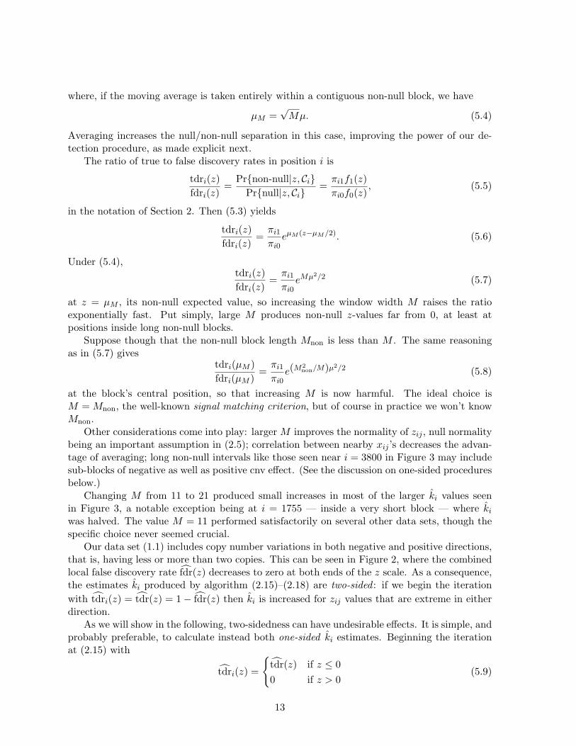
Figure 6: Solid histogram the 1500 zij values for positions i in 1750–1759, cnv data (1.1); line histogramfor the 748,500 other zij ; dotted curve cubic logistic regresssion estimate (5.12) for wi(z)/wi(0) (5.10)(multiplied by −5 for display).

14

Figure 6 and Figure 7 concern the application of (5.11) to the amalgamated set of positions1750 through 1759. The solid histogram in Figure 6 shows the 1500 zij at these 10 positionshaving an excess of negative values, compared to the distribution of all the rest. A logisticregression of the indicator

Iij =

{1 if i ∈ 1750 : 17590 otherwise

(5.12)

as a cubic function of zij gave estimate wi(z); the ratio wi(z)/wi(0) is plotted below the hori-zontal axis.

−6 −4 −2 0 2 4 6

0.0

0.2

0.4

0.6

0.8

1.0

z value

fdr

estim

ate

Method 1

Method 2

* * * * * * * * * * * * * **

*

*

*

*

*

*

*

*

*

**

* * * * * * * * * * * **

*

*

*

*

*

*

*

*

**

* * * * * * * * * * * *

low cn high cn

combined

Figure 7: Three estimates of the local false discovery rate for positions 1750–1759 of cnv data (1.1):combined from all 750,000 zij , as in Figure 2; Method 1 from 5 iterations of (2.15)–(2.18), two-sided;Method 2 from (5.11), using wi(z) as shown in Figure 6.

Three estimates fdri(z) for the local false discovery rate applying to positions 1750–1759appear in Figure 7: the combined estimate of Figure 2, obtained from all 750,000 zij values;Method 1, from five iterations of algorithm (2.15)–(2.18), applied in the two-sided fashion ofSection 2; and Method 2, from formula (5.11), with wi(z)/wi(0) as shown in Figure 6.

On the left side, both Method 1 and Method 2 yield much smaller estimates than thecombined curve, for instance fdri(−3) = 0.019 from Method 2, compared to the combinedestimate 0.125. Both Methods are adjusting the combined estimates fdr(zij) downward toaccount for the excess cnv activity observed at positions 1750–1759.

The story is different on the right side. Method 2 has fdri(z) = 1 for z > 0, which isintuitively correct since Figure 6 shows no tendency toward large positive z-values in positions1750–1759. Many of the other positions do show unusually large positive z-values, causing thecombined estimate fdr(z) to decline for large positive z. Method 1’s estimate declines evenmore sharply. It is using non-null density f1(z) (2.1) as estimated from the combined data, anddoes not “know” that the non-null values in positions 1750–1759 are only left-sided.

15

Applying Method 1 separately on the left and right, as in (5.9), resolves the discrepancywith Method 2. Method 2 itself tends to be noisy when applied to individual positions, and thetwo one-sided versions of Method 1 seem preferable in general.

6 Convergence Properties of the Iterative Algorithm

Algorithm (2.15)–(2.18) was stopped after five iterations since numerical convergence of theki values had nearly been achieved, producing the results pictured in Figure 3, Figure 4, andFigure 5. This section discusses the theoretical convergence point of the algorithm, leading to aformula for its standard error, and a connection with maximum likelihood estimation in model(3.7). The development will be in terms of πi1 = ki/n (2.16), rather than ki itself.

Returning to the two-groups notation of Section 2, let p1 and p0 = 1−p1 take values between0 and 1, and define

f(z, p1) = p1f1(z) + p0f0(z) (6.1)

andtdr(z, p1) =

p1f1(z)f(z, p1)

=1

1 + p0p1L(z)

(6.2)

where L(z) is the likelihood ratio

L(z) = f0(z)/f1(z). (6.3)

The actual true discovery rate in class Ci, Pr{non-null|z, Ci}, is

tdri(z) = tdr(z, πi1) = 1/

[1 + (πi0/πi1)L(z)] . (6.4)

(A little algebra shows that (6.4) equals (2.13).)Finally, define

hi(p1) = p1 −∫Z

tdr(z, p1)f(i)(z) dz (6.5)

where f(i)(z) equals f(z, πi1), the mixture distribution (2.9) of z in Ci, and the integral is takenover Z, the sample space of z. Since∫

Ztdr(z, πi1)f(i)(z) dz =

∫Z

πi1f1(z)f(i)(z)

f(i)(z) dz = πi1, (6.6)

the function hi(p1) satisfieshi(πi1) = 0; (6.7)

hi(·) will turn out to determine the convergence point of algorithm (2.15)–(2.18), and also thedelta-method standard error of the converged estimate.

Lemma 2. The derivative of hi(p1) is

h′i(p1) = 1−∫Z

tdr(z, p1) fdr(z, pi)f(i)(z) dz/p1p0 (6.8)

where fdr(z, p1) = 1− tdr(z, p1) (6.2).

16

Proof. From (6.2), we calculate

∂ tdr(z, p1)∂p1

=1[

1 +(

1p1− 1)L(z)

]2 L(z)p21

=tdr(z, p1)2

p21

f0(z)f1(z)

=tdr(z, p1)

p21

p1f1(z)f(z, p1)

f0(z)f1(z)

=tdr(z, p1) fdr(z, p1)

p1p0

(6.9)

which gives (6.8) from (6.2). �

The derivative h′(p1) takes on a convenient form at p1 = πi1 (the actual non-null probabilityin class Ci), where hi(πi1) = 0.

Lemma 3.h′i(πi1) = ξi/πi1πi0 (6.10)

withξi =

∫Z

[tdr(z, πi1)− πi1]2 f(i)(z) dz, (6.11)

the variance of tdr(z, πi1) = tdri(z) in Ci (which is also the variance of fdri(z) in Ci).

Proof. Define I to be the null indicator for a random case in Ci,

I =

{1 if null0 if non-null,

(6.12)

soπi1 = Pr{I = 0|Ci} and tdri(z) = Pr{I = 0|zi, Ci}. (6.13)

At p1 = πi1, (6.8) becomes

h′i(πi1) = 1−∫Z

tdri(z) fdri(z)f(i)(z) dz/πi1πi0. (6.14)

But tdri(z) fdri(z) equals vari{I|z}, the conditional variance of the Bernoulli random variableI, so

h′i(πi1) = 1− Ei {vari{I|z}} /πi1πi0, (6.15)

Ei indicating expectation with respect to f(i)(z).A standard relationship between conditional and unconditional variances is

vari{I} = Ei {vari{I|z}}+ vari {Ei{I|z}} , (6.16)

vari indicating variance with respect to f(i)(z). Since Ei{I|z} = fdri(z), (6.15)–(6.16) implyh′i(πi1) = vari{fdri(z)}/πi1πi0, which is the same as (6.10). �

Note. Since πi1πi0 = vari{I}, we can also write (6.8) as

h′i(πi1) = vari {Ei{I|z}} / vari{I} ≤ 1. (6.17)

17

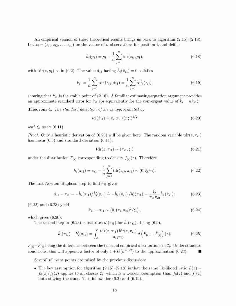
An empirical version of these theoretical results brings us back to algorithm (2.15)–(2.18).Let zi = (zi1, zi2, . . . , zin) be the vector of n observations for position i, and define

hi(p1) = p1 −1n

n∑j=1

tdr(zij , p1), (6.18)

with tdr(z, p1) as in (6.2). The value πi1 having hi(πi1) = 0 satisfies

πi1 =1n

n∑j=1

tdr (zij , πi1) =1n

n∑j=1

tdri(zij), (6.19)

showing that πi1 is the stable point of (2.16). A familiar estimating-equation argument providesan approximate standard error for πi1 (or equivalently for the convergent value of ki = nπi1).

Theorem 4. The standard deviation of πi1 is approximated by

sd (πi1) .= πi1πi0/(nξi)1/2 (6.20)

with ξi as in (6.11).

Proof. Only a heuristic derivation of (6.20) will be given here. The random variable tdr(z, πi1)has mean (6.6) and standard deviation (6.11),

tdr(z, πi1) ∼ (πi1, ξi) (6.21)

under the distribution F(i) corresponding to density f(i)(z). Therefore

hi(πi1) = πi1 −1n

n∑j=1

tdr(zij , πi1) ∼ (0, ξi/n). (6.22)

The first Newton–Raphson step to find πi1 gives

πi1 − πi1 = −hi(πi1)/h′i(πi1) .= −hi (πi1)

/h′i(πi1) =

ξiπi1πi0

hi (πi1) ; (6.23)

(6.22) and (6.23) yieldπi1 − πi1 ∼

(0, (πi1πi0)2/ξi

), (6.24)

which gives (6.20).The second step in (6.23) substitutes h′i(πi1) for h′i(πi1). Using (6.9),

h′i(πi1)− h′i(πi1) =∫Z

tdr(z, πi1) fdr(z, πi1)πi1πi0

d(F(i) − F(i)

)(z), (6.25)

F(i)−F(i) being the difference between the true and empirical distributions in Ci. Under standardconditions, this will append a factor of only 1 +O(n−1/2) to the approximation (6.23). �

Several relevant points are raised by the previous discussion:

• The key assumption for algorithm (2.15)–(2.18) is that the same likelihood ratio L(z) =f0(z)/f1(z) applies to all classes Ci, which is a weaker assumption than f0(z) and f1(z)both staying the same. This follows for (6.2) and (6.19).

18

• The stable point πi1 (6.19) can be found by Newton–Raphson updating, dp1 = −hi(p1)/h′i(p1),(6.18) and (6.8). Theoretically, this should converge faster than the EM-type steps in(2.15)–(2.18).

• The convergence estimates ki = nπi were nearly the same as those shown in Figure 3, forexample 39.3 compared to 39.1 at position 1755.

• The standard deviation estimates for ki based on the empirical version of (6.20) were agood match to those in Figure 5 for positions having ki ≥ 15. However, (6.20) gave quiteerratic results for ki < 15, and is not recommended in general.

• The standard deviation estimate (6.20) equals the Cramer–Rao lower bound at r = 1 inparametric family (3.7), but not for r 6= 1.

• A possible competitor to πi1 would be

πi1 = π1ri (6.26)

where ri is the maximum likelihood estimate of r in (3.4), (3.7). Example 7 of Efron(1975) implies that πi1 would be fully efficient at r = 1 but far more variable than Fisherinformation calculations suggest when r much exceeds 1.

• For our cnv example (1.1), the ML estimates πi1 were a nearly perfect linear function ofthe converged iterative estimates πi1,

πi1.= 1.06 · πi1. (6.27)

In other words, the ki estimates of Figure 3 nearly equal MLEs from the class-wise two-groups model (2.1), (2.8).

7 Identifying CNV-Prone Regions in Tumors

Analysis of chromosome copy number aberrations in tumor samples is now a staple of cancerstudies. A central question in this paper has been “Which locations are more prone to be gainedor lost?” The meaning and motivation of this question in the analysis of tumor samples differsfrom that in the analysis of normal samples. Since tumorigenesis involves the breakdown ofDNA repair and maintenance systems, the accumulation of many chromosomal gains and lossesin tumors are hypothesized to be random events that occur as a due effect of the developmentof the tumor. In this sense, many of the cnas we detect are “passenger” mutations, that, unlike“driver” mutations, do not play a functional role in driving tumor progression. For a recentreview, see Stratton, Campbell and Futreal (2009). An important goal in the analysis of tumorsamples is to find the driver mutations. Since passenger mutations tend to occur more or lessrandomly throughout the genome, and driver mutations tend to favor certain genome positionscontaining functionally relevant genes, driver mutations can be identified by finding positionsthat are more cna-prone than “random” in a cross-sample analysis. This is the scientific problemthat motivates our analysis of tumor samples.

As an example, we analyze chromosome 1 of 207 glioblastoma subjects from the CancerGenome Atlas project (The Cancer Genome Atlas, 2008). This data is a 42,075 by 207 matrix,derived from the 42,075 probes that map to chromosome 1 on the Illumina HumanHap 550k

19

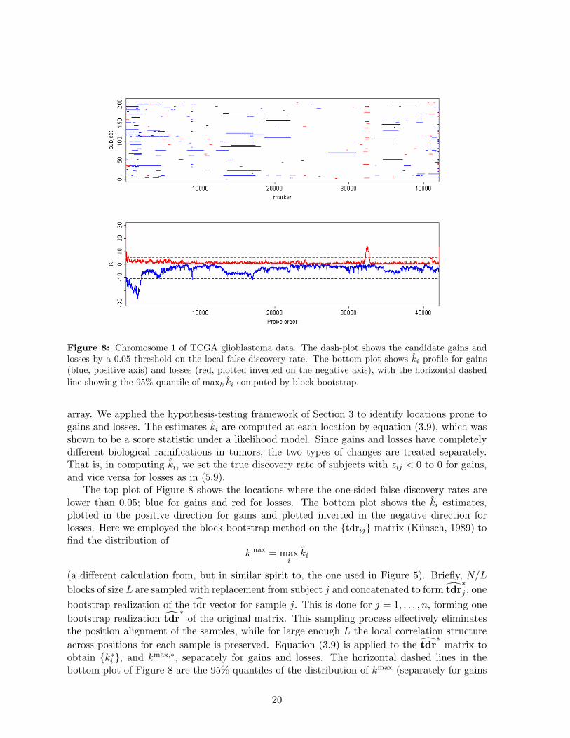
Figure 8: Chromosome 1 of TCGA glioblastoma data. The dash-plot shows the candidate gains andlosses by a 0.05 threshold on the local false discovery rate. The bottom plot shows ki profile for gains(blue, positive axis) and losses (red, plotted inverted on the negative axis), with the horizontal dashedline showing the 95% quantile of maxk ki computed by block bootstrap.

array. We applied the hypothesis-testing framework of Section 3 to identify locations prone togains and losses. The estimates ki are computed at each location by equation (3.9), which wasshown to be a score statistic under a likelihood model. Since gains and losses have completelydifferent biological ramifications in tumors, the two types of changes are treated separately.That is, in computing ki, we set the true discovery rate of subjects with zij < 0 to 0 for gains,and vice versa for losses as in (5.9).

The top plot of Figure 8 shows the locations where the one-sided false discovery rates arelower than 0.05; blue for gains and red for losses. The bottom plot shows the ki estimates,plotted in the positive direction for gains and plotted inverted in the negative direction forlosses. Here we employed the block bootstrap method on the {tdrij} matrix (Kunsch, 1989) tofind the distribution of

kmax = maxiki

(a different calculation from, but in similar spirit to, the one used in Figure 5). Briefly, N/Lblocks of size L are sampled with replacement from subject j and concatenated to form tdr

∗j , one

bootstrap realization of the tdr vector for sample j. This is done for j = 1, . . . , n, forming onebootstrap realization tdr

∗of the original matrix. This sampling process effectively eliminates

the position alignment of the samples, while for large enough L the local correlation structureacross positions for each sample is preserved. Equation (3.9) is applied to the tdr

∗matrix to

obtain {k∗i }, and kmax,∗, separately for gains and losses. The horizontal dashed lines in thebottom plot of Figure 8 are the 95% quantiles of the distribution of kmax (separately for gains

20

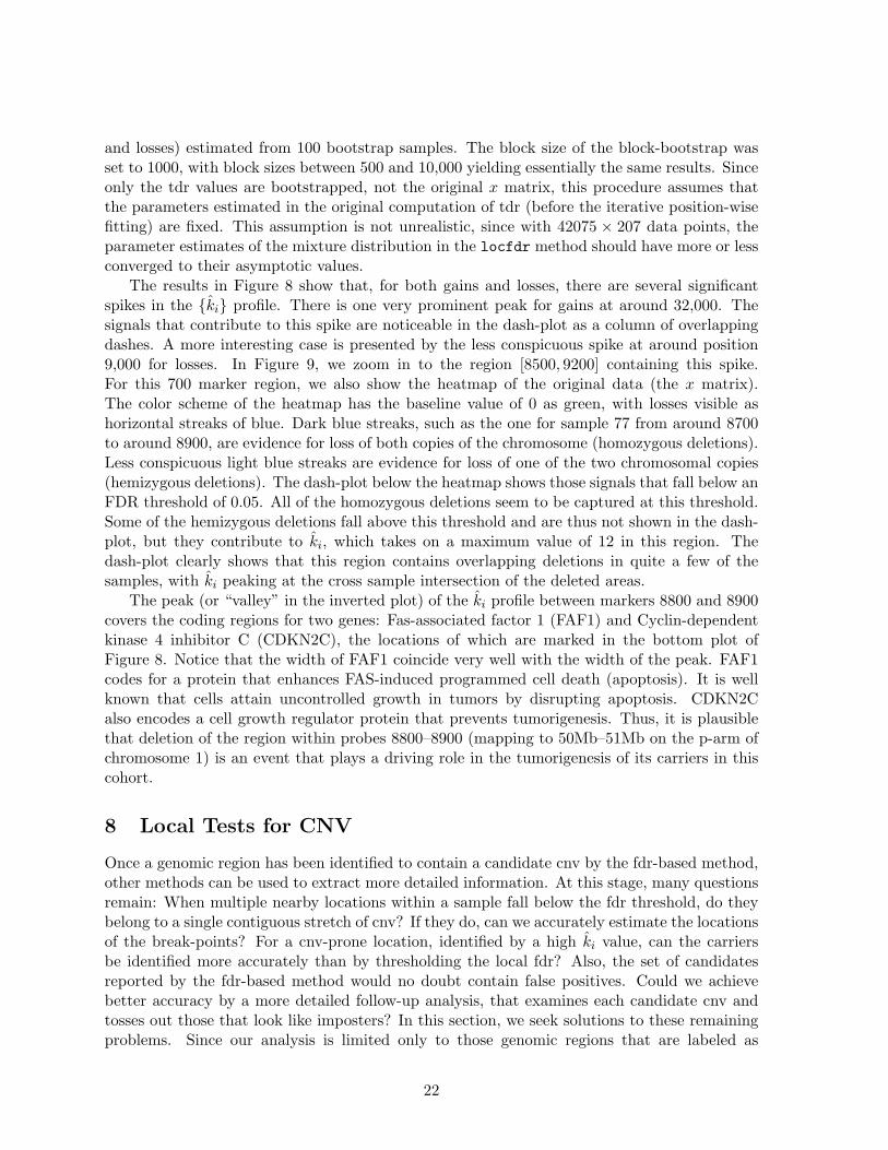
Figure 9: The region between 8500 and 9200 of Chromosome 1 of TCGA glioblastoma data. Theheatmap on top shows the Illumina log ratios. The dash-plot in the middle shows the candidate gainsand losses by a 0.05 threshold on the local false discovery rate. The bottom plot shows ki profile forgains (blue, positive axis) and losses (red, negative axis), with the horizontal dashed line showing the95% quantile of maxk ki computed by block bootstrap. The locations of the genes FAF1 and CDKN2Care shown in the bottom plot.

21

and losses) estimated from 100 bootstrap samples. The block size of the block-bootstrap wasset to 1000, with block sizes between 500 and 10,000 yielding essentially the same results. Sinceonly the tdr values are bootstrapped, not the original x matrix, this procedure assumes thatthe parameters estimated in the original computation of tdr (before the iterative position-wisefitting) are fixed. This assumption is not unrealistic, since with 42075 × 207 data points, theparameter estimates of the mixture distribution in the locfdr method should have more or lessconverged to their asymptotic values.

The results in Figure 8 show that, for both gains and losses, there are several significantspikes in the {ki} profile. There is one very prominent peak for gains at around 32,000. Thesignals that contribute to this spike are noticeable in the dash-plot as a column of overlappingdashes. A more interesting case is presented by the less conspicuous spike at around position9,000 for losses. In Figure 9, we zoom in to the region [8500, 9200] containing this spike.For this 700 marker region, we also show the heatmap of the original data (the x matrix).The color scheme of the heatmap has the baseline value of 0 as green, with losses visible ashorizontal streaks of blue. Dark blue streaks, such as the one for sample 77 from around 8700to around 8900, are evidence for loss of both copies of the chromosome (homozygous deletions).Less conspicuous light blue streaks are evidence for loss of one of the two chromosomal copies(hemizygous deletions). The dash-plot below the heatmap shows those signals that fall below anFDR threshold of 0.05. All of the homozygous deletions seem to be captured at this threshold.Some of the hemizygous deletions fall above this threshold and are thus not shown in the dash-plot, but they contribute to ki, which takes on a maximum value of 12 in this region. Thedash-plot clearly shows that this region contains overlapping deletions in quite a few of thesamples, with ki peaking at the cross sample intersection of the deleted areas.

The peak (or “valley” in the inverted plot) of the ki profile between markers 8800 and 8900covers the coding regions for two genes: Fas-associated factor 1 (FAF1) and Cyclin-dependentkinase 4 inhibitor C (CDKN2C), the locations of which are marked in the bottom plot ofFigure 8. Notice that the width of FAF1 coincide very well with the width of the peak. FAF1codes for a protein that enhances FAS-induced programmed cell death (apoptosis). It is wellknown that cells attain uncontrolled growth in tumors by disrupting apoptosis. CDKN2Calso encodes a cell growth regulator protein that prevents tumorigenesis. Thus, it is plausiblethat deletion of the region within probes 8800–8900 (mapping to 50Mb–51Mb on the p-arm ofchromosome 1) is an event that plays a driving role in the tumorigenesis of its carriers in thiscohort.

8 Local Tests for CNV

Once a genomic region has been identified to contain a candidate cnv by the fdr-based method,other methods can be used to extract more detailed information. At this stage, many questionsremain: When multiple nearby locations within a sample fall below the fdr threshold, do theybelong to a single contiguous stretch of cnv? If they do, can we accurately estimate the locationsof the break-points? For a cnv-prone location, identified by a high ki value, can the carriersbe identified more accurately than by thresholding the local fdr? Also, the set of candidatesreported by the fdr-based method would no doubt contain false positives. Could we achievebetter accuracy by a more detailed follow-up analysis, that examines each candidate cnv andtosses out those that look like imposters? In this section, we seek solutions to these remainingproblems. Since our analysis is limited only to those genomic regions that are labeled as

22

“interesting” by the fdr method, we will call the ensuing analysis “local”, as opposed to a“global” analysis covering the entire data matrix.

In the local analysis, we return to the original {xij} matrix of normalized intensity values.The fdr method described in the previous sections works off the matrix of z-values, which wereobtained from the normalized data through a smoothing step that averages adjacent probes.The original x matrix, if properly normalized, contains entries that are approximately i.i.d.standard normal under the null hypothesis. An effective normalization procedure based on alow-rank factorization followed by probe-specific standardization is given in Siegmund et al.(2010).

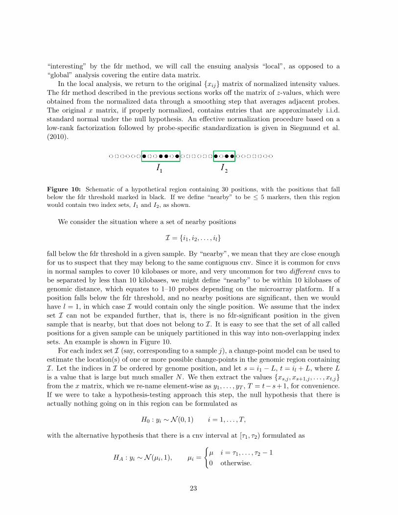
Figure 10: Schematic of a hypothetical region containing 30 positions, with the positions that fallbelow the fdr threshold marked in black. If we define “nearby” to be ≤ 5 markers, then this regionwould contain two index sets, I1 and I2, as shown.

We consider the situation where a set of nearby positions

I = {i1, i2, . . . , il}

fall below the fdr threshold in a given sample. By “nearby”, we mean that they are close enoughfor us to suspect that they may belong to the same contiguous cnv. Since it is common for cnvsin normal samples to cover 10 kilobases or more, and very uncommon for two different cnvs tobe separated by less than 10 kilobases, we might define “nearby” to be within 10 kilobases ofgenomic distance, which equates to 1–10 probes depending on the microarray platform. If aposition falls below the fdr threshold, and no nearby positions are significant, then we wouldhave l = 1, in which case I would contain only the single position. We assume that the indexset I can not be expanded further, that is, there is no fdr-significant position in the givensample that is nearby, but that does not belong to I. It is easy to see that the set of all calledpositions for a given sample can be uniquely partitioned in this way into non-overlapping indexsets. An example is shown in Figure 10.

For each index set I (say, corresponding to a sample j), a change-point model can be used toestimate the location(s) of one or more possible change-points in the genomic region containingI. Let the indices in I be ordered by genome position, and let s = i1 − L, t = il + L, where Lis a value that is large but much smaller N . We then extract the values {xs,j , xs+1,j , . . . , xt,j}from the x matrix, which we re-name element-wise as y1, . . . , yT , T = t− s+ 1, for convenience.If we were to take a hypothesis-testing approach this step, the null hypothesis that there isactually nothing going on in this region can be formulated as

H0 : yi ∼ N (0, 1) i = 1, . . . , T,

with the alternative hypothesis that there is a cnv interval at [τ1, τ2) formulated as

HA : yi ∼ N (µi, 1), µi =

{µ i = τ1, . . . , τ2 − 10 otherwise.

23

The parameters µ, τ1, τ2 are not known. For some platforms, it has been noted that the noisevariance increases for CNV regions, which may motivate the addition of an extra variance termσ2 to the observations within [τ1, τ2) under the alternative. However, we have found, as doesOlshen et al. (2004) and Wen et al. (2006), that the heterogeneous variance model does notsignificantly improve detection accuracy.

Figure 11: Example of a local cnv analysis. This region contains probes 3400–4200 of sample 41 of thedata shown in Figure 1. The vertical axis is the normalized (but unsmoothed) intensity values (the xij ’s).The red points are locations with fdr < 0.05, and the black points are locations with fdr < 0.005. Thevertical lines show the change-points determined by the modified BIC method (Zhang and Siegmund,2007).

Under the above model, the generalized likelihood ratio assuming known τ1, τ2 and maxi-mized over µ has the form

L(τ1, τ2) =τ2−1∑i=τ1

yi/

(τ2 − τ1).

Maximizing over τ1 and τ2, the generalized likelihood ratio test of H0 versus HA is L(τ1, τ2),where

(τ1, τ2) = argmax1≤τ1<τ2≤M L(τ1, τ2).

The CBS algorithm of Olshen et al. (2004) and the MBIC method of Zhang and Siegmund(2007) use a similar statistic, but adjusted for an unknown baseline mean. Significance valuesfor tests using L(τ1, τ2) are given in Siegmund (2007). Since this region has already passed aglobal filter based on fdr, a less conservative test is more appropriate for the local analysis.In our experience, thresholds of 0.05 or 0.1, without adjusting for the multiple testing acrossregions, work well. Since the set of regions reported by the fdr procedure should be heavilyenriched for true cnvs, it seems more fitting to treat the analysis of each region as an estimationproblem rather than as a testing problem. Instead of asking the question, “Is there a CNV inthis region?” we instead ask, “How many break-points does this region contain, and whatare their locations?” This framework is especially fitting for index sets that contain multiplecnvs, or complex variants with nested changes. In this sense, the BIC approach described inYao (1988) and Zhang and Siegmund (2007) seems to be appropriate. The models in Yao(1988) and Zhang and Siegmund (2007) assume that there are m change-points τ1, . . . , τm (mis unknown). The data is assumed Gaussian, with the mean shifting at each change-point,but with the variance remaining constant. While Yao (1988) showed that the traditional BIC

24

(Schwarz, 1978) is consistent for the estimation of m, Zhang and Siegmund (2007) showed thatit is not consistent in estimating the Bayes factor, the quantity that underlies the classic BIC.Zhang and Siegmund (2007) gave a modified form of the BIC, which improves the small-sampleaccuracy for estimating m.

An example, shown in Figure 11, is the well-known cnv region on the p-arm of chromosome22. The figure shows the break-points estimated by maximum likelihood under this Gaussianmodel, with the number of break-points estimated using the modified BIC criterion of Zhangand Siegmund (2007). As indicated by the coloring of points, while most of the locations inthe nested homozygous deletion (between 559 and 578) pass the 0.005 fdr threshold, some ofthe locations in the hemizygous deletion (between 337 and 559) do not even pass the 0.05threshold. Thus, a local change-point analysis is useful for refining the fdr result and buildinga more complete picture for each cnv region.

The BIC may report that the candidate region contains no change-points. There would betwo possible reasons for this: the region is a false positive, or the signal is so weak that it ismissed by the local analysis. Local analysis with a well formulated change-point model shouldbe more powerful than global analyses, because the multiplicity has been much reduced. Thus,if the BIC reports 0 change-points, we conclude that the region is a false positive.

References

Beroukhim, R., Getz, G., Nghiemphu, L., Barretina, J., Hsueh, T., Linhart, D., Vivanco, I.,Lee, J. C., Huang, J. H., Alexander, S., Du, J., Kau, T., Thomas, R. K., Shah, K., Soto, H.,Perner, S., Prensner, J., Debiasi, R. M., Demichelis, F., Hatton, C., Rubin, M. A., Garraway,L. A., Nelson, S. F., Liau, L., Mischel, Cloughesy, T. F., Meyerson, M., Golub, T. A., Lander,E. S., Mellinghoff, I. K. and Sellers, W. R. (2007). Assessing the significance of chromosomalaberrations in cancer: Methodology and application to glioma. Proc. Natl. Acad. Sci. USA :0710052104+.

Bignell, G. R., Huang, J., Greshock, J., Watt, S., Butler, A., West, S., Grigorova, M., Jones,K. W., Wei, W., Stratton, M. R., Futreal, P. A., Weber, B., Shapero, M. H. and Wooster,R. (2004). High-resolution analysis of DNA copy number using oligonucleotide microarrays.Genome Res. 14: 287–295.

Conrad, D., Andrews, T., Carter, N., Hurles, M., and Pritchard, J. (2006). A high-resolutionsurvey of deletion polymorphism in the human genome. Nat. Genet. 38: 75–81.

Diskin, S. J., Eck, T., Greshock, J., Mosse, Y. P., Naylor, T., Stoeckert Jr., C. J., Weber,B. L., Maris, J. M. and Grant, G. R. (2006). Stac: A method for testing the significanceof DNA copy number aberrations across multiple array-cgh experiments. Genome Res. 16:1149–1158.

Efron, B. (1975). Defining the curvature of a statistical problem (with applications to secondorder efficiency). Ann. Statist. 3: 1189–1242, with a discussion by C. R. Rao, Don A. Pierce,D. R. Cox, D. V. Lindley, Lucien LeCam, J. K. Ghosh, J. Pfanzagl, Niels Keiding, A. P.Dawid, Jim Reeds and with a reply by the author.

Efron, B. (2008). Microarrays, empirical Bayes and the two-groups model. Statist. Sci. 23: 1–22.

25

Efron, B. (2009). Empirical bayes estimates for large-scale prediction problems. J. Amer. Statist.Assoc. 104: 1015–1028.

Efron, B. (2010a). Correlated z-values and the accuracy of large-scale statistical estimates. J.Amer. Statist. Assoc. To appear.

Efron, B. (2010b). Large-Scale Inference: Empirical Bayes Methods for Estimation, Testing,and Prediction, Institute of Mathematical Statistics Monographs I . Cambridge: CambridgeUniversity Press, to be published August 2010.

Guttman, M., Mies, C., Dudycz-Sulicz, K., Diskin, S. J., Baldwin, D. A., Stoeckert, C. J. andGrant, G. R. (2007). Assessing the significance of conserved genomic aberrations using highresolution genomic microarrays. PLoS Genetics 3: e143+.

Kunsch, H. (1989). The jackknife and the bootstrap for general stationary observations. Ann.Statist. 17: 1217–1241.

Lai, W. R., Johnson, M. D., Kucherlapati, R. and Park, P. J. (2005). Comparative analysisof algorithms for identifying amplifications and deletions in array-CGH data. Bioinformatics21: 3763–3770.

McKernan, K. J., Peckham, H. E., Costa, G. L., McLaughlin, S. F., Fu, Y., Tsung, E. F.,Clouser, C. R., Duncan, C., Ichikawa, J. K., Lee, C. C., Zhang, Z., Ranade, S. S., Dimalanta,E. T., Hyland, F. C., Sokolsky, T. D., Zhang, L., Sheridan, A., Fu, H., Hendrickson, C. L.,Li, B., Kotler, L., Stuart, J. R., Malek, J. A., Manning, J. M., Antipova, A. A., Perez, D. S.,Moore, M. P., Hayashibara, K. C., Lyons, M. R., Beaudoin, R. E., Coleman, B. E., Laptewicz,M. W., Sannicandro, A. E., Rhodes, M. D., Gottimukkala, R. K., Yang, S., Bafna, V., Bashir,A., MacBride, A., Alkan, C., Kidd, J. M., Eichler, E. E., Reese, M. G., De La Vega, F. M. andBlanchard, A. P. (2009). Sequence and structural variation in a human genome uncovered byshort-read, massively parallel ligation sequencing using two-base encoding. Genome Res. 19:1527–1541.

Mills, R. E. E., Luttig, C. T. T., Larkins, C. E. E., Beauchamp, A., Tsui, C., Pittard, W. S. S.and Devine, S. E. E. (2006). An initial map of insertion and deletion (indel) variation in thehuman genome. Genome Res 16: 1182–1190.

Newton, M., Gould, M., Reznikoff, C. and Haag, J. (1998). On the statistical analysis of allelic-loss data. Stat. Med. 17: 1425–1445.

Newton, M. and Lee, Y. (2000). Inferring the location and effect of tumor suppressor genes byinstability-selection modeling of allelic-loss data. Biometrics 56: 1088–1097.

Olshen, A. B., Venkatraman, E. S., Lucito, R. and Wigler, M. (2004). Circular binary segmen-tation for the analysis of array-based DNA copy number data. Biostatistics 5: 557–572.

Peiffer, D. A., Le, J. M., Steemers, F. J., Chang, W., Jenniges, T., Garcia, F., Haden, K., Li,J., Shaw, C. A., Belmont, J., Cheung, S. W., Shen, R. M., Barker, D. L. and Gunderson,K. L. (2006). High-resolution genomic profiling of chromosomal aberrations using infiniumwhole-genome genotyping. Genome Res. 16: 1136–1148.

26

Pinkel, D., Segraves, R., Sudar, D., Clark, S., Poole, I., Kowbel, D., Collins, C., Kuo, W. L.,Chen, C., Zhai, Y., Dairkee, S. H., Ljung, B. M., Gray, J. W. and Albertson, D. G. (1998).High resolution analysis of DNA copy number variation using comparative genomic hybridiza-tion to microarrays. Nat. Genet. 20: 207–11.

Pollack, J., Perou, C., Alizadeh, A., Eisen, M., Pergamenschikov, A., Williams, C., Jeffrey,S., Botstein, D. and Brown, P. (1999). Genome-wide analysis of DNA copy-number changesusing cDNA microarrays. Nat. Genet. 23: 41–46.

Robbins, H. (1956). An empirical Bayes approach to statistics. In Proceedings of the ThirdBerkeley Symposium on Mathematical Statistics and Probability, 1954–1955, vol. I . Berkeleyand Los Angeles: University of California Press, 157–163.

Rouveirol, C., Stransky, N., Hupe, P., La Rosa, P., Viara, E., Barillot, E. and Radvanyi,F. (2006). Computation of recurrent minimal genomic alterations from array-CGH data.Bioinformatics 22: 849–856.

Schwarz, G. (1978). Estimating the dimension of a model. Ann. Statist. 6: 461–464.

Siegmund, D., Yakir, B. and Zhang, N. (2010). Detecting simultaneous variant intervals inaligned sequences, submitted.

Siegmund, D. O. (2007). Approximate tail probabilities for the maxima of some random fields.Ann. Probab. 16: 487–501.

Snijders, A. M., Nowak, N., Segraves, R., Blackwood, S., Brown, N., Conroy, J., Hamilton, G.,Hindle, A. K., Huey, B., Kimura, K., Law, S., Myambo, K., Palmer, J., Ylstra, B., Yue, J. P.,Gray, J. W., Jain, A. N., Pinkel, D. and Albertson, D. G. (2001). Assembly of microarraysfor genome-wide measurement of DNA copy number. Nat. Genet. 29: 263–264.

Stratton, M. R., Campbell, P. J. and Futreal, P. A. (2009). The cancer genome. Nature 458:719–724.

Taylor, B. S., Barretina, J., Socci, N. D., Decarolis, P., Ladanyi, M., Meyerson, M., Singer, S.and Sander, C. (2008). Functional copy-number alterations in cancer. PLoS ONE 3: e3179+.

The Cancer Genome Atlas (2008). Comprehensive genomic characterization defines humanglioblastoma genes and core pathways. Nature 455: 1061–1068.

Wang, P., Kim, Y., Pollack, J., Narasimhan, B. and Tibshirani, R. (2005). A method for callinggains and losses in array-CGH data. Biostatistics 6: 45–58.

Wen, C., Wu, Y., Huang, Y., Chen, W., Liu, S., Jiang, S., Juang, J., Lin, C., Fang, W., Hsiung,C. and Chang, I. (2006). A Bayes regression approach to array-CGH data. Stat. Appl. Mol.Biol. 5.

Willenbrock, H. and Fridlyand, J. (2005). A comparison study: Applying segmentation toarray-CGH data for downstream analyses. Bioinformatics 21: 4084–4091.

Yao, Y.-C. (1988). Estimating the number of change-points via Schwarz’ criterion. Stat. Probab.Lett. 6: 181–189.

27

Zhang, N. (2010). DNA Copy Number Profiling in Normal and Tumor Genomes. In Fu, W.(ed.), Probability and Statistics and Their Applications to Biology . Springer-Verlag.

Zhang, N. and Siegmund, D. (2007). A modified Bayes information criterion with applicationsto the analysis of comparative genomic hybridization data. Biometrics 63: 22–32.

Zhang, N., Siegmund, D., Ji, H. and Li, J. Z. (2010). Detecting simultaneous change-points inmultiple sequences. Biometrika In press.

28