Fall 2015 Math 283 Prof. Teslergptesler/283/slides/pca_15-handout.pdf · 31.9702 -16.5683-16.5683 13.0018 = s XX s XY s YX s ... Prof. Tesler Principal Components Analysis Math 283

Principal Components Analysis (PCA)and Singular Value Decomposition (SVD)

with applications to Microarrays

Prof. Tesler

Math 283Fall 2015

Prof. Tesler Principal Components Analysis Math 283 / Fall 2015 1 / 39

Covariance

Let X and Y be random variables, possibly dependent.Recall that the covariance of X and Y is defined as

Cov(X, Y) = E((X − µX)(Y − µY)

)and that an alternate formula is

Cov(X, Y) = E(XY) − E(X)E(Y)

Previously we used

Var(X + Y) = Var(X) + Var(Y) + 2 Cov(X, Y)

andVar(X1 + X2 + · · ·+ Xn) = Var(X1) + · · ·+ Var(Xn)


Covariance properties

Covariance propertiesCov(X, X) = Var(X)

Cov(X, Y) = Cov(Y, X)

Cov(aX + b, cY + d) = ac Cov(X, Y)

Sign of covariance Cov(X, Y) = E((X − µX)(Y − µY))

When Cov(X, Y) is positive:there is a tendency to have X > µX when Y > µY and vice-versa,and X < µX when Y < µY and vice-versa.When Cov(X, Y) is negative:there is a tendency to have X > µX when Y < µY and vice-versa,and X < µX when Y > µY and vice-versa.When Cov(X, Y) = 0:a) X and Y might be independent, but it’s not guaranteed.b) Var(X + Y) = Var(X) + Var(Y)


Sample variance

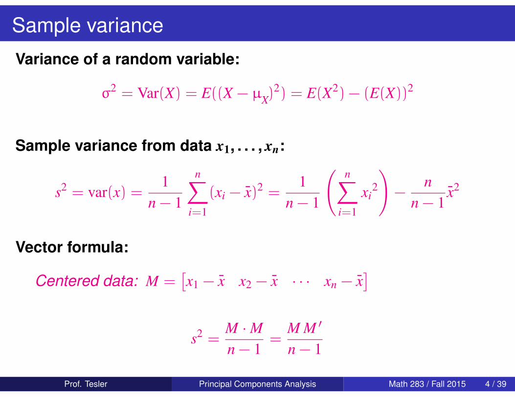
Variance of a random variable:

σ2 = Var(X) = E((X − µX)2) = E(X2) − (E(X))2

Sample variance from data x1, . . . , xn:

s2 = var(x) =1

n − 1

n∑i=1

(xi − x)2 =1

n − 1

(n∑

i=1

xi2

)−

nn − 1

x2

Vector formula:

Centered data: M =[x1 − x x2 − x · · · xn − x

]s2 =

M ·Mn − 1

=M M ′

n − 1


Sample covariance

Covariance between random variables X, Y:

σXY = Cov(X, Y) = E((X − µX)(Y − µY)) = E(XY) − E(X)E(Y)

Sample covariance from data (x1, y1), . . . , (xn, yn):

sXY = cov(x, y) =1

n − 1

n∑i=1

(xi − x)(yi − y) =1

n − 1

(n∑

i=1

xiyi

)−

nn − 1

xy

Vector formula:

MX =[x1 − x x2 − x · · · xn − x

]MY =

[y1 − y y2 − y · · · yn − y

]sXY =

MX ·MY

n − 1=

MX M ′Yn − 1


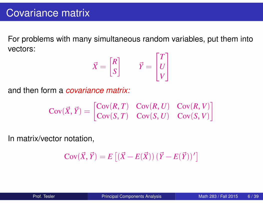
Covariance matrix

For problems with many simultaneous random variables, put them intovectors:

~X =

[RS

]~Y =

TUV

and then form a covariance matrix:

Cov(~X, ~Y) =[

Cov(R, T) Cov(R, U) Cov(R, V)Cov(S, T) Cov(S, U) Cov(S, V)

]

In matrix/vector notation,

Cov(~X, ~Y) = E[(~X − E(~X)) (~Y − E(~Y)) ′

]


Covariance matrix (a.k.a. Variance-Covariance matrix)

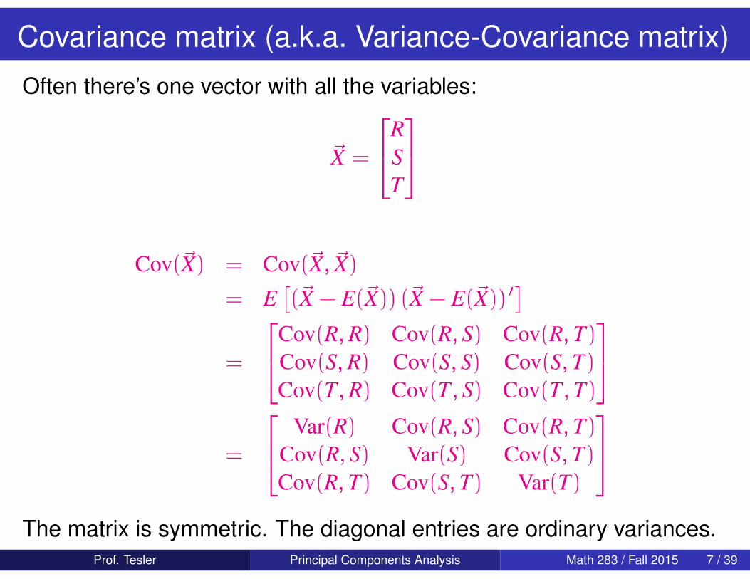
Often there’s one vector with all the variables:

~X =

RST

Cov(~X) = Cov(~X, ~X)= E

[(~X − E(~X)) (~X − E(~X)) ′

]=

Cov(R, R) Cov(R, S) Cov(R, T)Cov(S, R) Cov(S, S) Cov(S, T)Cov(T, R) Cov(T, S) Cov(T, T)

=

Var(R) Cov(R, S) Cov(R, T)Cov(R, S) Var(S) Cov(S, T)Cov(R, T) Cov(S, T) Var(T)

The matrix is symmetric. The diagonal entries are ordinary variances.


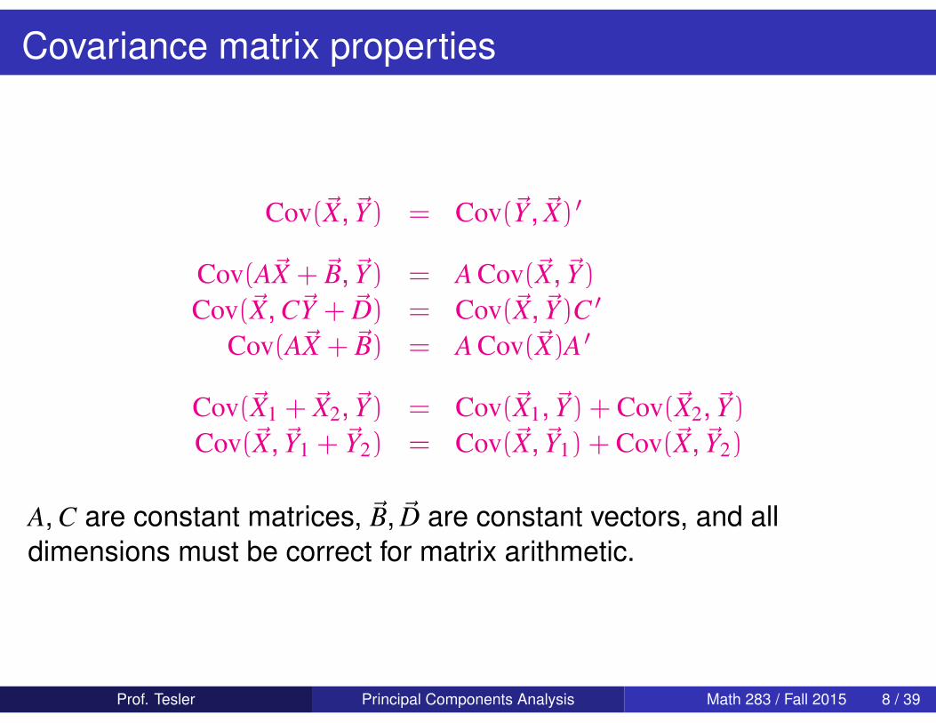
Covariance matrix properties

Cov(~X, ~Y) = Cov(~Y, ~X) ′

Cov(A~X + ~B, ~Y) = A Cov(~X, ~Y)Cov(~X, C~Y + ~D) = Cov(~X, ~Y)C ′

Cov(A~X + ~B) = A Cov(~X)A ′

Cov(~X1 + ~X2, ~Y) = Cov(~X1, ~Y) + Cov(~X2, ~Y)Cov(~X, ~Y1 + ~Y2) = Cov(~X, ~Y1) + Cov(~X, ~Y2)

A, C are constant matrices, ~B, ~D are constant vectors, and alldimensions must be correct for matrix arithmetic.


Example (2D, but works for higher dimensions too)

Data (x1, y1), . . . , (x100, y100):

M0 =

[x1 · · · x100y1 · · · y100

]=

[3.0858 0.8806 9.8850 · · · 4.410612.8562 10.7804 8.7504 · · · 13.5627

]

!5 0 5 10 150

2

4

6

'

10

12

14

16

1'

20(ri+inal data


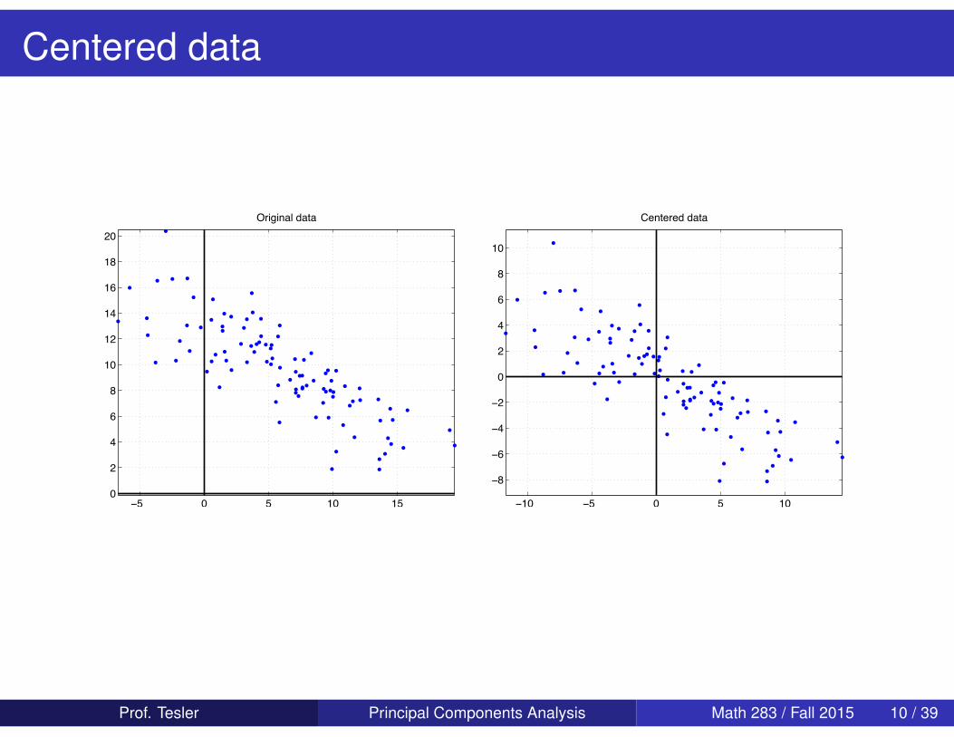
Centered data

!5 0 5 10 150

2

4

6

'

10

12

14

16

1'

20(ri+inal data

!10 !5 0 5 10

!8

!6

!4

!2

0

2

4

6

8

10

Centered data


Computing sample covariance matrix

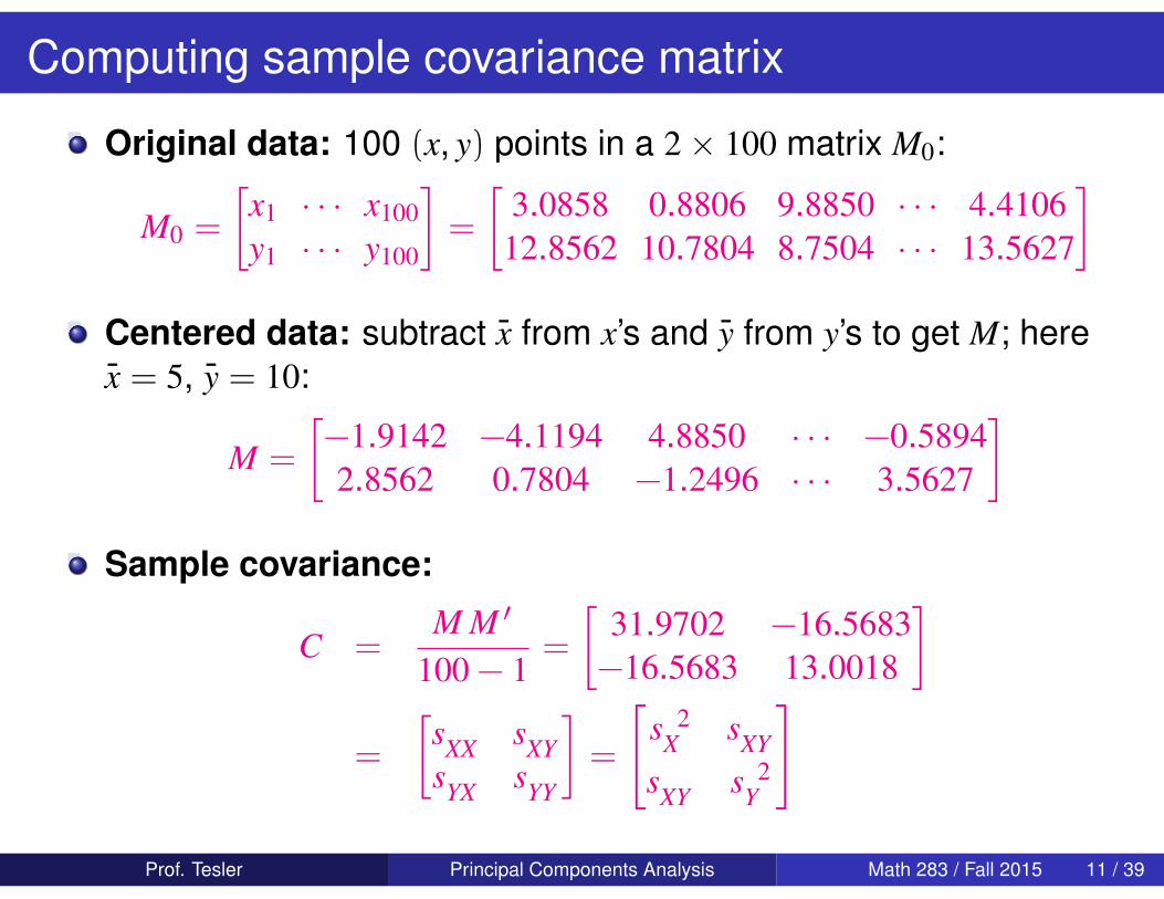
Original data: 100 (x, y) points in a 2× 100 matrix M0:

M0 =

[x1 · · · x100y1 · · · y100

]=

[3.0858 0.8806 9.8850 · · · 4.410612.8562 10.7804 8.7504 · · · 13.5627

]Centered data: subtract x from x’s and y from y’s to get M; herex = 5, y = 10:

M =

[−1.9142 −4.1194 4.8850 · · · −0.58942.8562 0.7804 −1.2496 · · · 3.5627

]Sample covariance:

C =M M ′

100 − 1=

[31.9702 −16.5683−16.5683 13.0018

]=

[sXX sXYsYX sYY

]=

[sX

2 sXY

sXY sY2

]


Orthonormal matrix

Recall that for vectors ~v, ~w, we have ~v · ~w = |~v| |~w| cos(θ),where θ is the angle between the vectors.

Orthogonal means perpendicular.~v and ~w are orthogonal when the angle between them isθ = 90◦ = π

2 radians. So cos(θ) = 0 and ~v · ~w = 0.

Vectors ~v1, . . . ,~vn are orthonormal when~vi ·~vj = 0 for i , j (different vectors are orthogonal)~vi ·~vi = 1 for all i (each vector has length 1; they are all unit vectors)

In short: ~vi ·~vj = δij =

{0 if i , j1 if i = j.


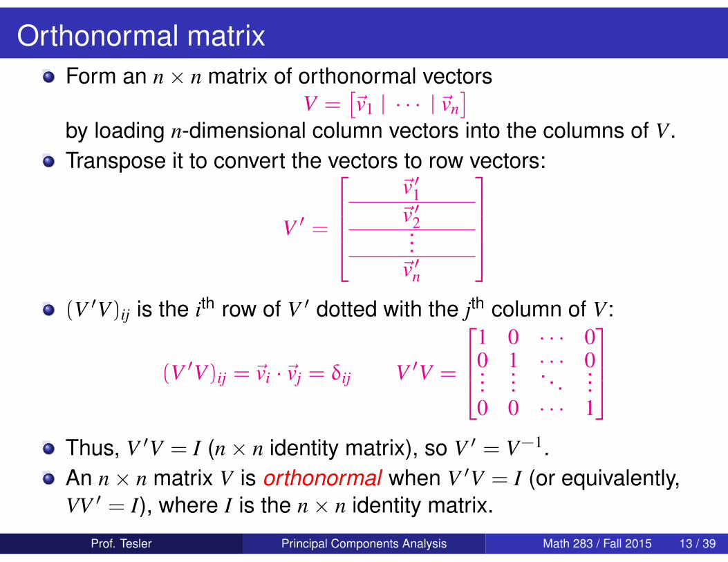
Orthonormal matrixForm an n× n matrix of orthonormal vectors

V =[~v1 | · · · | ~vn

]by loading n-dimensional column vectors into the columns of V.Transpose it to convert the vectors to row vectors:

V ′ =

~v ′1~v ′2...~v ′n

(V ′V)ij is the ith row of V ′ dotted with the jth column of V:

(V ′V)ij = ~vi ·~vj = δij V ′V =

1 0 · · · 00 1 · · · 0...

.... . .

...0 0 · · · 1

Thus, V ′V = I (n× n identity matrix), so V ′ = V−1.An n× n matrix V is orthonormal when V ′V = I (or equivalently,VV ′ = I), where I is the n× n identity matrix.


Diagonalizing the sample covariance matrix C

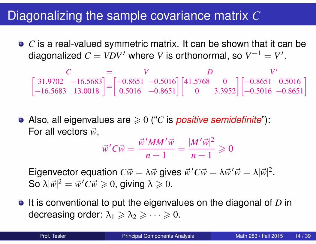
C is a real-valued symmetric matrix. It can be shown that it can bediagonalized C = VDV ′ where V is orthonormal, so V−1 = V ′.

C = V D V ′[31.9702 −16.5683−16.5683 13.0018

]=

[−0.8651 −0.50160.5016 −0.8651

][41.5768 0

0 3.3952

][−0.8651 0.5016−0.5016 −0.8651

]

Also, all eigenvalues are > 0 (“C is positive semidefinite”):For all vectors ~w,

~w ′C~w =~w ′MM ′~w

n − 1=

|M ′~w|2

n − 1> 0

Eigenvector equation C~w = λ~w gives ~w ′C~w = λ~w ′~w = λ|~w|2.So λ|~w|2 = ~w ′C~w > 0, giving λ > 0.

It is conventional to put the eigenvalues on the diagonal of D indecreasing order: λ1 > λ2 > · · · > 0.


Principal axes

The columns of V are the right eigenvectors of C.Multiply each eigenvector by the square root of its eigenvalue toget the principal components.

Eigenvalue Eigenvector PC

41.5768[−0.86510.5016

] [−5.57823.2343

]3.3952

[−0.5016−0.8651

] [−0.9242−1.5940

]Put them into the columns of a matrix:

P = V√

D =

[−5.5782 −0.92423.2343 −1.5940

]

C = VDV ′ = V√

D√

D ′V ′ = (V√

D)(V√

D) ′ = PP ′


Principal axes

Plot the centered data with lines along the principal axes:

!10 !5 0 5 10

!8

!6

!4

!2

0

2

4

6

8

10

Principal axes

Sum of squared perpendicular distances of data points to first PCline (red) is minimum among all lines through origin.ith PC is perpendicular to the previous ones, and the sum ofsquared perpendicular distances to the span (line, plane, ...) ofthe first i PCs is minimum among all i-dim. spaces through origin.


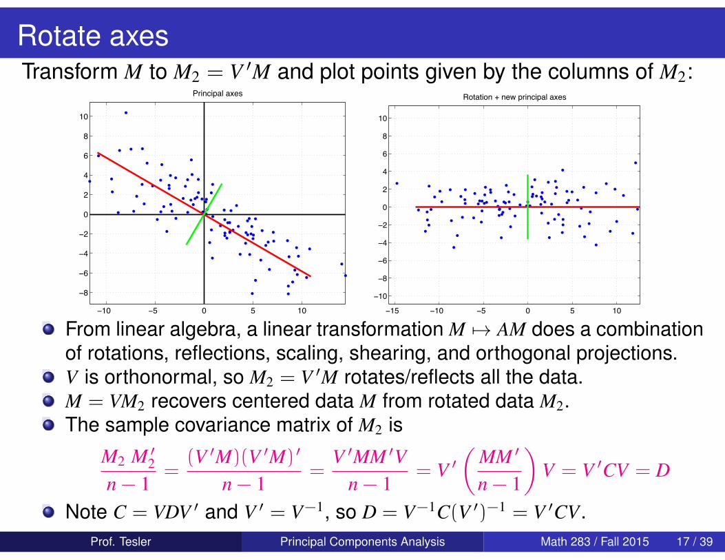
Rotate axesTransform M to M2 = V ′M and plot points given by the columns of M2:

!10 !5 0 5 10

!8

!6

!4

!2

0

2

4

6

8

10

Principal axes

!15 !10 !5 0 5 10

!10

!$

!%

!4

!2

0

2

4

%

$

10

(ot+tion / ne1 prin4ip+5 +6es

From linear algebra, a linear transformation M 7→ AM does a combinationof rotations, reflections, scaling, shearing, and orthogonal projections.V is orthonormal, so M2 = V ′M rotates/reflects all the data.M = VM2 recovers centered data M from rotated data M2.The sample covariance matrix of M2 is

M2 M ′2n − 1

=(V ′M)(V ′M) ′

n − 1=

V ′MM ′Vn − 1

= V ′(

MM ′

n − 1

)V = V ′CV = D

Note C = VDV ′ and V ′ = V−1, so D = V−1C(V ′)−1 = V ′CV.Prof. Tesler Principal Components Analysis Math 283 / Fall 2015 17 / 39

New coordinates

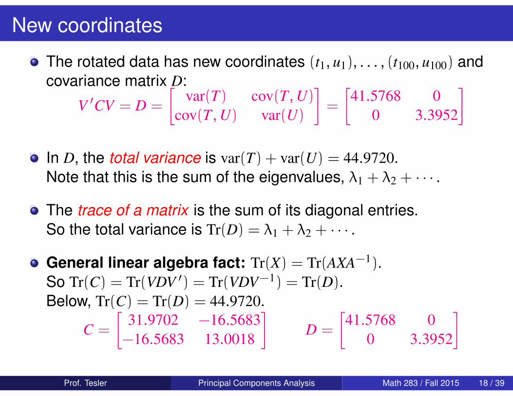
The rotated data has new coordinates (t1, u1), . . . , (t100, u100) andcovariance matrix D:

V ′CV = D =

[var(T) cov(T, U)

cov(T, U) var(U)

]=

[41.5768 0

0 3.3952

]

In D, the total variance is var(T) + var(U) = 44.9720.Note that this is the sum of the eigenvalues, λ1 + λ2 + · · · .

The trace of a matrix is the sum of its diagonal entries.So the total variance is Tr(D) = λ1 + λ2 + · · · .

General linear algebra fact: Tr(X) = Tr(AXA−1).So Tr(C) = Tr(VDV ′) = Tr(VDV−1) = Tr(D).Below, Tr(C) = Tr(D) = 44.9720.

C =

[31.9702 −16.5683−16.5683 13.0018

]D =

[41.5768 0

0 3.3952

]


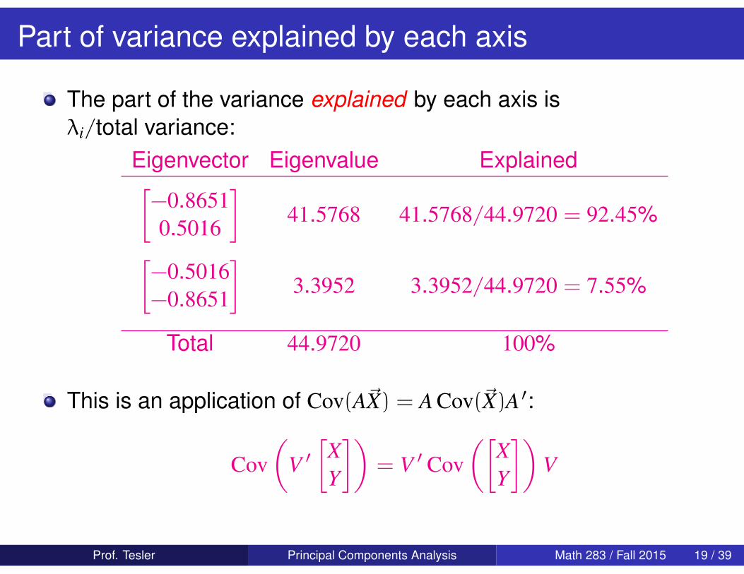
Part of variance explained by each axis

The part of the variance explained by each axis isλi/total variance:

Eigenvector Eigenvalue Explained[−0.86510.5016

]41.5768 41.5768/44.9720 = 92.45%[

−0.5016−0.8651

]3.3952 3.3952/44.9720 = 7.55%

Total 44.9720 100%

This is an application of Cov(A~X) = A Cov(~X)A ′:

Cov(

V ′[

XY

])= V ′ Cov

([XY

])V


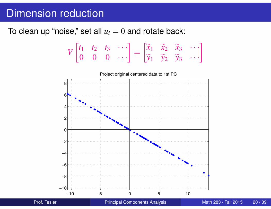
Dimension reduction

To clean up “noise,” set all ui = 0 and rotate back:

V[

t1 t2 t3 · · ·0 0 0 · · ·

]=

[x1 x2 x3 · · ·y1 y2 y3 · · ·

]

!10 !5 0 5 10!10

!$

!%

!4

!2

0

2

4

%

$

(ro+ect ori1inal centered data to 1st (C


Dimension reduction

Say we want to keep enough information to explain 90% of thevariance.

Take enough top PCs to explain > 90% of the variance.

Let M3 be M2 (rotated data) with the remaining coordinates zeroedout.

Rotate it back to the original axes with VM3.

In other applications, a dominant signal can be suppressed byzeroing out the coordinates for the top PCs instead of the bottomPCs.


Variations for PCA (and SVD, upcoming)

Some people reverse the roles of rows and columns of M.

In some applications, M is “centered” (subtract off row means) andin others, it’s not.

If the ranges on the variables (rows) are very different, the datamight be rescaled in each row to make similar ranges. Forexample, replace each row by Z-scores for the row.


Sensitivity to scaling

PCA was originally designed for measurements in ordinary space,so all axes had the same units (e.g., cm or inches) and equivalentresults would be obtained no matter what units were used.It’s problematic to mix physical quantities with different units:

Length of (a, b) in (seconds,mm):√

a2 + b2

(adding sec2 plus mm2 is not legitimate!)

Convert to (hours,miles):∣∣( a

3600 , b1609344

)∣∣ = √a2

36002 +b2

16093442

Angles are also distorted by this unit conversion:arctan(b/a) , arctan

(a

3600

/b

1609344

).

|(0 ◦C, 0 ◦C)| = 0 vs. |(32 ◦F, 32 ◦F)| = 32√

2.Both ◦C and ◦F use an arbitrary “zero” instead of absolute zero.

PCA is sensitive to differences in the scale, offset, and ranges ofthe variables. Rescaling one row w/o the others changes anglesand lengths nonuniformly, and changes eigenvalues andeigenvectors in an inequivalent way.Typically addressed by replacing each row with Z-scores.


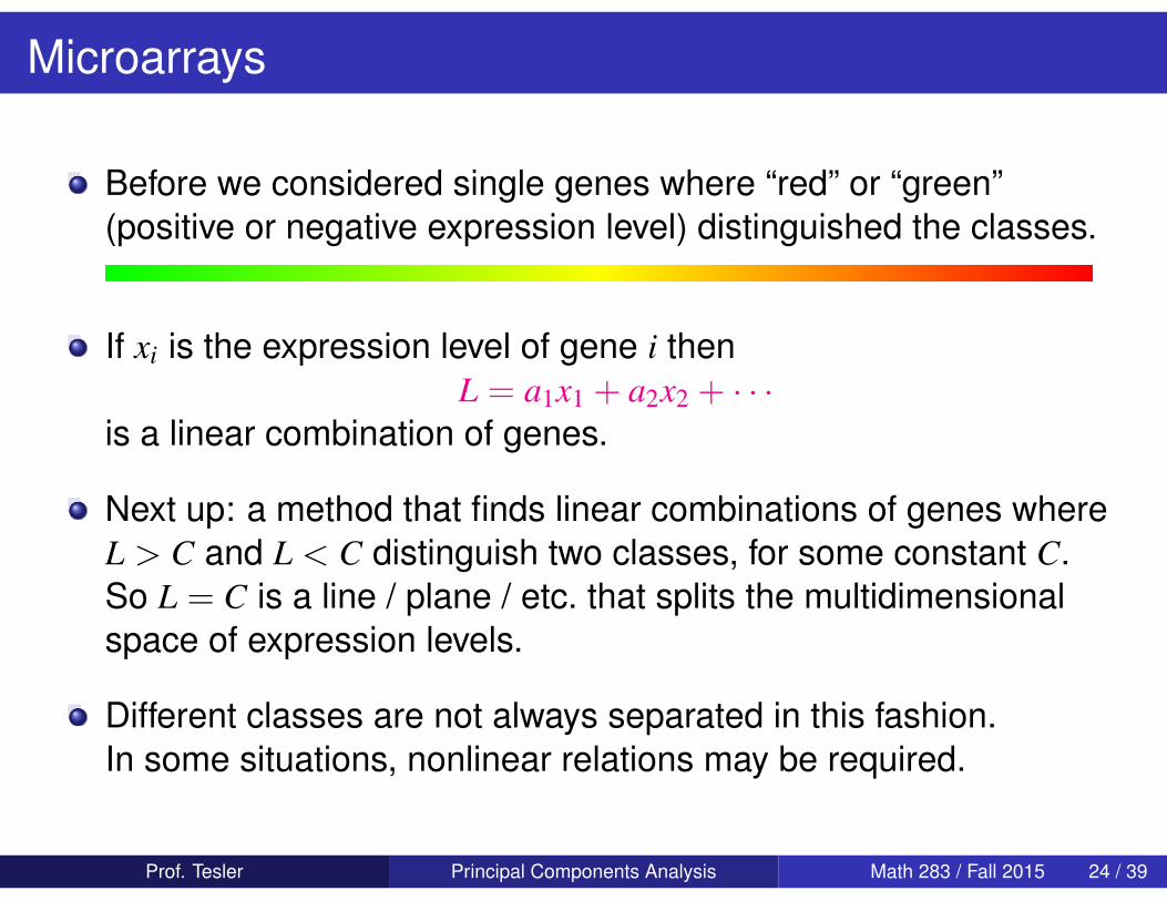
Microarrays

Before we considered single genes where “red” or “green”(positive or negative expression level) distinguished the classes.

If xi is the expression level of gene i thenL = a1x1 + a2x2 + · · ·

is a linear combination of genes.

Next up: a method that finds linear combinations of genes whereL > C and L < C distinguish two classes, for some constant C.So L = C is a line / plane / etc. that splits the multidimensionalspace of expression levels.

Different classes are not always separated in this fashion.In some situations, nonlinear relations may be required.


Microarrays

Consider an experiment with 80 microarrays, each with 10000 spots.

M is 10000× 80.

C = MM ′80−1 is 10000× 10000!

M ′M is 80× 80.

We will see that MM ′ has the same 80 eigenvalues as M ′M, plusan additional 10000 − 80 = 9920 eigenvalues equal to 0.

Some of the 80 eigenvalues of M ′M may also be 0.For centered data, all row sums of M are 0 so [1, . . . , 1] ′ is aneigenvector of M ′M with eigenvalue 0.

We will see we can work with the smaller of MM ′ or M ′M.


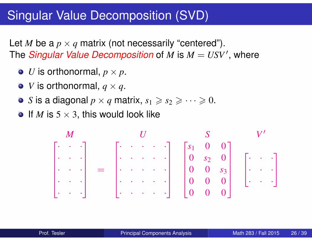
Singular Value Decomposition (SVD)

Let M be a p× q matrix (not necessarily “centered”).The Singular Value Decomposition of M is M = USV ′, where

U is orthonormal, p× p.V is orthonormal, q× q.S is a diagonal p× q matrix, s1 > s2 > · · · > 0.If M is 5× 3, this would look like

M U S V ′· · ·· · ·· · ·· · ·· · ·

=

· · · · ·· · · · ·· · · · ·· · · · ·· · · · ·

s1 0 00 s2 00 0 s30 0 00 0 0

· · ·· · ·· · ·


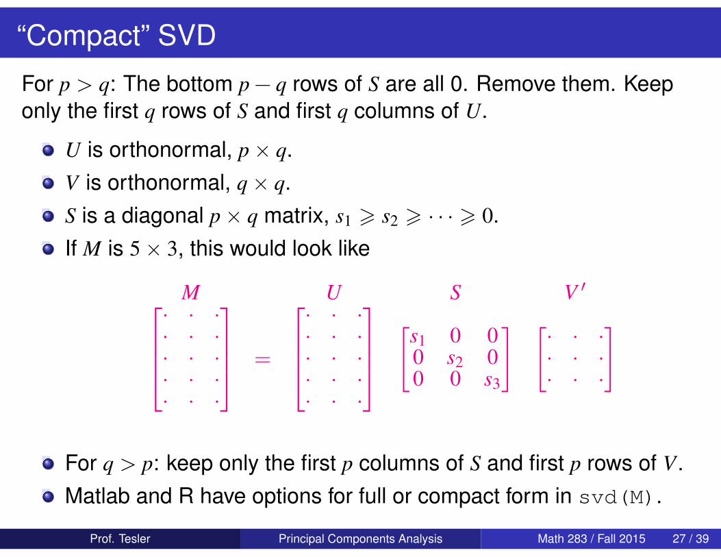
“Compact” SVD

For p > q: The bottom p − q rows of S are all 0. Remove them. Keeponly the first q rows of S and first q columns of U.

U is orthonormal, p× q.V is orthonormal, q× q.S is a diagonal p× q matrix, s1 > s2 > · · · > 0.If M is 5× 3, this would look like

M U S V ′· · ·· · ·· · ·· · ·· · ·

=

· · ·· · ·· · ·· · ·· · ·

[

s1 0 00 s2 00 0 s3

] [· · ·· · ·· · ·

]

For q > p: keep only the first p columns of S and first p rows of V.Matlab and R have options for full or compact form in svd(M).


Computing the SVD

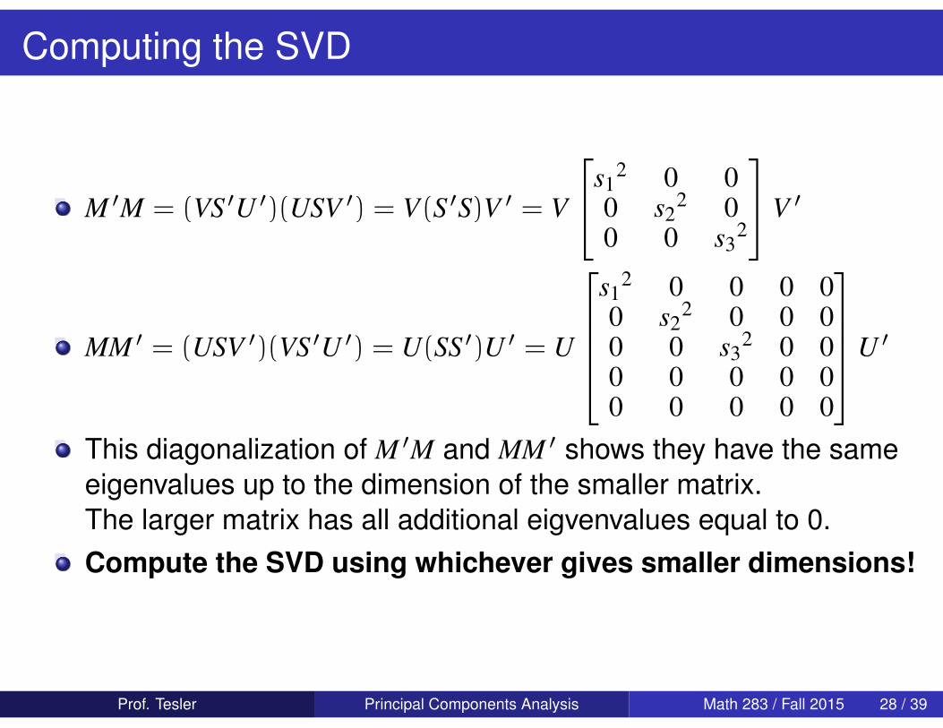
M ′M = (VS ′U ′)(USV ′) = V(S ′S)V ′ = V

s12 0 0

0 s22 0

0 0 s32

V ′

MM ′ = (USV ′)(VS ′U ′) = U(SS ′)U ′ = U

s1

2 0 0 0 00 s2

2 0 0 00 0 s3

2 0 00 0 0 0 00 0 0 0 0

U ′

This diagonalization of M ′M and MM ′ shows they have the sameeigenvalues up to the dimension of the smaller matrix.The larger matrix has all additional eigvenvalues equal to 0.Compute the SVD using whichever gives smaller dimensions!


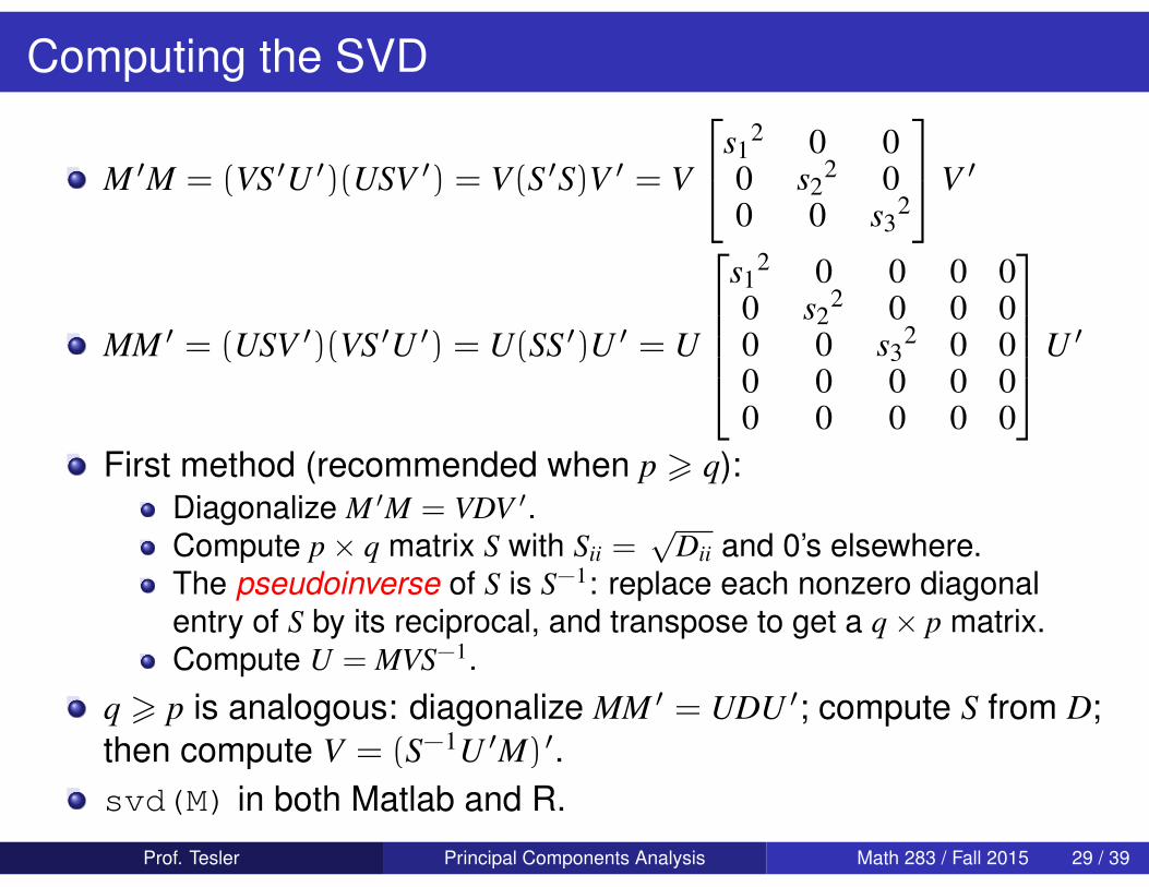
Computing the SVD

M ′M = (VS ′U ′)(USV ′) = V(S ′S)V ′ = V

s12 0 0

0 s22 0

0 0 s32

V ′

MM ′ = (USV ′)(VS ′U ′) = U(SS ′)U ′ = U

s1

2 0 0 0 00 s2

2 0 0 00 0 s3

2 0 00 0 0 0 00 0 0 0 0

U ′

First method (recommended when p > q):Diagonalize M ′M = VDV ′.Compute p× q matrix S with Sii =

√Dii and 0’s elsewhere.

The pseudoinverse of S is S−1: replace each nonzero diagonalentry of S by its reciprocal, and transpose to get a q× p matrix.Compute U = MVS−1.

q > p is analogous: diagonalize MM ′ = UDU ′; compute S from D;then compute V = (S−1U ′M) ′.svd(M) in both Matlab and R.


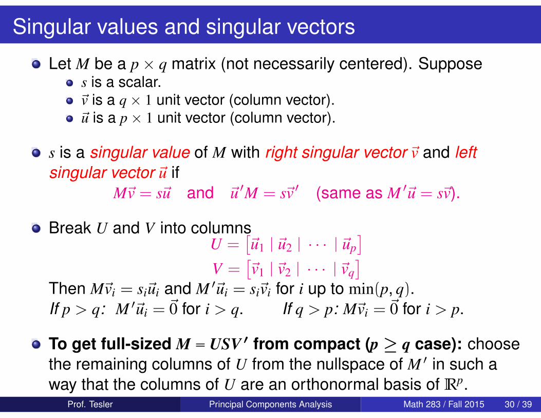
Singular values and singular vectors

Let M be a p× q matrix (not necessarily centered). Supposes is a scalar.~v is a q× 1 unit vector (column vector).~u is a p× 1 unit vector (column vector).

s is a singular value of M with right singular vector ~v and leftsingular vector ~u if

M~v = s~u and ~u ′M = s~v ′ (same as M ′~u = s~v).

Break U and V into columnsU =

[~u1 | ~u2 | · · · | ~up

]V =

[~v1 | ~v2 | · · · | ~vq

]Then M~vi = si~ui and M ′~ui = si~vi for i up to min(p, q).If p > q: M ′~ui = ~0 for i > q. If q > p: M~vi = ~0 for i > p.

To get full-sized M = USV ′ from compact (p ≥ q case): choosethe remaining columns of U from the nullspace of M ′ in such away that the columns of U are an orthonormal basis of Rp.


Relation between PCA and SVD

Previous computation for PCAStart with centered data matrix M (n columns).Compute covariance matrix, diagonalize it, compute P:

C =MM ′

n − 1= VDV ′ = PP ′ where P = V

√D

Computing PCA using SVDIn terms of the SVD factorization M = USV ′, covariance is

C =MM ′

n − 1=

(USV ′)(VS ′U ′)n − 1

=U(SS ′)U ′

n − 1= UDU ′ where D = SS ′

n−1

= PP ′ where P = US√n−1

Variance for ith component is si2

n−1

Note: there were minor notation adjustments to deal with n − 1.


SVD in microarrays

Nielsen et al.1 studied tumors in six types of tissue.41 tissue samples and 46 microarray slidesThey switched microarray platforms in the middle of theexperiment:

The first 26 slides have 22,654 spots (22K).The next 20 slides have 42,611 spots (42K) (mostly a superset).Five of the samples were done on both 22K and 42K platforms.

7425 spots were in common to both platforms, had good signalacross all slides, and had sample variance above a certainthreshold. So M is 7425× 46.

1Molecular characterisation of soft tissue tumours: a gene expression study,Lancet (2002) 359: 1301–1307.


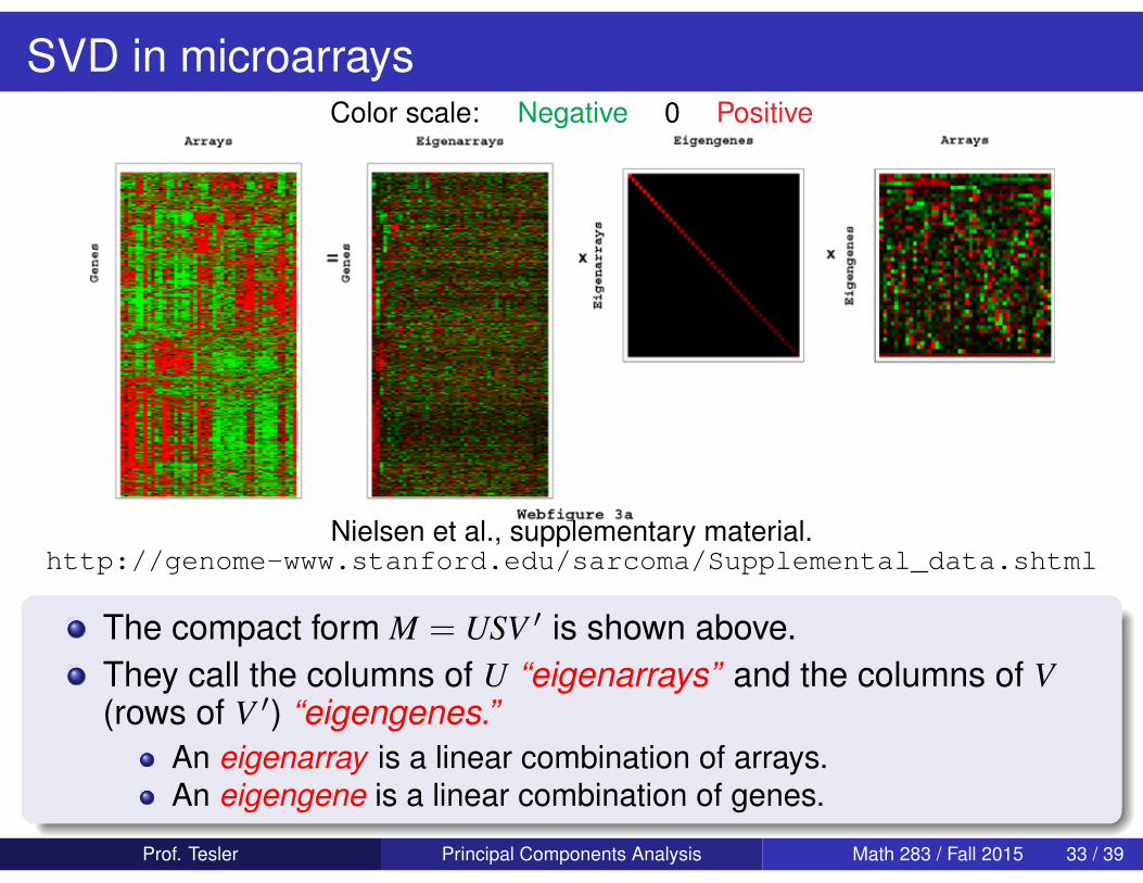
SVD in microarraysColor scale: Negative 0 Positive

Nielsen et al., supplementary material.http://genome-www.stanford.edu/sarcoma/Supplemental_data.shtml

The compact form M = USV ′ is shown above.They call the columns of U “eigenarrays” and the columns of V(rows of V ′) “eigengenes.”

An eigenarray is a linear combination of arrays.An eigengene is a linear combination of genes.


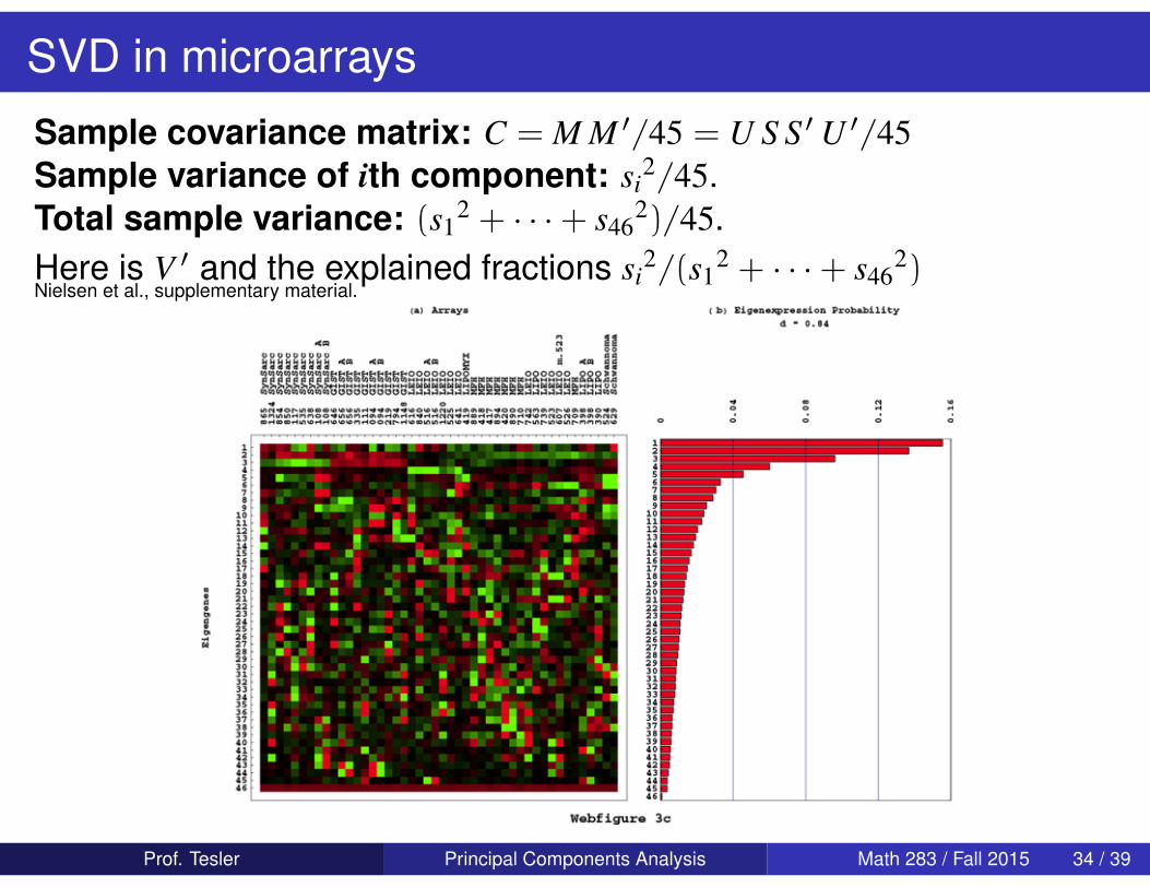
SVD in microarrays

Sample covariance matrix: C = M M ′/45 = U S S ′U ′/45Sample variance of ith component: si

2/45.Total sample variance: (s1

2 + · · ·+ s462)/45.

Here is V ′ and the explained fractions si2/(s1

2 + · · ·+ s462)

Nielsen et al., supplementary material.


“Expression level” of eigengenes

The expression level of gene i on array j is Mij.

Interpretation of change of basis S = U ′MV:the ith eigenarray only detects the ith eigengene, and has 0response to other eigengenes.

Interpretation of V ′ = U ′MS−1:The “expression level” of eigengene i on array j is (V ′)ij = Vji.

Let ~m represent a new array (e.g., a column vector of expressionlevels in each gene).The expression level of eigengene i is (U ′~m)i/si.


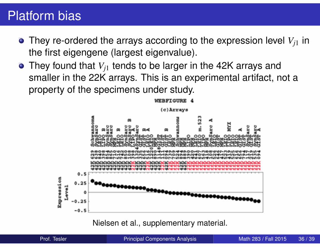
Platform bias

They re-ordered the arrays according to the expression level Vj1 inthe first eigengene (largest eigenvalue).They found that Vj1 tends to be larger in the 42K arrays andsmaller in the 22K arrays. This is an experimental artifact, not aproperty of the specimens under study.

Nielsen et al., supplementary material.


Removing 22K vs. 42K array bias

Let S be S with the (1,1) entry replaced by 0.

Let M = USV ′.

This reduces the signal and variance in many spots.After removing weak spots, they cut down to 5520 spots, giving a5520× 46 data matrix.


Classification — Eigengenes — 1DFor the 5520× 46 matrix, the expression levels of the top threeeigengenes can be used to classify some tumor types.

!2 !1 0 1 2$ 104

'((656 !+,'( -'((094 !+,'( /

'((850 !'1n'arc'((656 !+,'( /'((094 !+,'( -

'((638 !'1n'arc'((535 !'1n'arc'((854 !'1n'arc'((117 !'1n'arc

'((219 !+,'('((335 !+,'(

'((865 !'1n'arc'((794 !+,'('((646 !+,'('((111 !+,'(

'((108 !'1n'arc -'((1148!+,'(

'((108 !'1n'arc /'((1324!'1n'arc

'((516 !89,: -'((516 !89,: /

'((840 !89,:'((1220!89,:'((525 !89,:'((390 !8,;:

'((419 !8,;:<=>?'((616 !89,:'((418 !=FA'((889 !=FA'((641 !89,:

'((629 !'cBCannoEa'((417 !=FA'((890 !=FA

'((398 !8,;: -'((742 !89,: '((894 !=FA'((739 !89,:

'((398 !8,;: /'((523 !89,:'((563 !8,;:

'((524 !'cBCannoEa'((420 !=FA'((710 !=FA

'((607 !89,: E.523'((526 !89,:'((709 !=FA

5520 spots eigengene 1

!1 !0.5 0 0.5 1 1.5x 104

STT094 !GIST ASTT794 !GISTSTT219 !GISTSTT335 !GISTSTT646 !GIST

STT094 !GIST BSTT656 !GIST B

STT1148!GISTSTT656 !GIST A

STT629 !SchwannomaSTT111 !GIST

STT524 !SchwannomaSTT710 !MFHSTT840 !LEIO

STT398 !LIPO ASTT398 !LIPO B

STT641 !LEIOSTT709 !MFH

STT742 !LEIO STT516 !LEIO BSTT516 !LEIO A

STT526 !LEIOSTT739 !LEIOSTT890 !MFHSTT616 !LEIOSTT420 !MFH

STT419 !LIPO/MYXSTT894 !MFH

STT607 !LEIO m.523STT390 !LIPOSTT563 !LIPO

STT1220!LEIOSTT417 !MFHSTT889 !MFHSTT523 !LEIOSTT525 !LEIO

STT1324!SynSarcSTT865 !SynSarc

STT418 !MFHSTT854 !SynSarc

STT108 !SynSarc BSTT108 !SynSarc A

STT638 !SynSarcSTT850 !SynSarcSTT117 !SynSarcSTT535 !SynSarc

5520 spots eigengene 2

!!"### !!#### !"### # "###

$%%"!&'!()*+',$%%&!&'!()*+

$%%"!&'!()*+'-$%%&.!'!()*+$%%/.#'!()*+$%%"0"'!()*+$%%!00#!()*+

$%%.!1'!(*2+3456$%%"07'!()*+$%%//1'!489$%%.!:'!489

$%%#1.'!;*$%',$%%/&"'!$<=$>?@$%%!!!'!;*$%

$%%#1.'!;*$%'-$%%&7/'!$<=$>?@$%%!!./!;*$%

$%%/"#'!$<=$>?@$%%&#:'!()*+'AB"07

$%%/".'!$<=$>?@$%%0!1'!;*$%$%%.!/'!489

$%%!70.!$<=$>?@$%%71#'!(*2+

$%%"7"'!$<=$>?@$%%&"&'!;*$%'-$%%77"'!;*$%$%%:1.'!;*$%

$%%!!:'!$<=$>?@$%%"0.'!$@CD>==EA>

$%%.0#'!489$%%&"&'!;*$%',$%%/1#'!489$%%:.0'!()*+'

$%%&01'!$@CD>==EA>$%%"0&'!()*+$%%/1.'!489$%%:71'!()*+

$%%!#/'!$<=$>?@',$%%&.&'!;*$%$%%"&7'!(*2+$%%:!#'!489$%%:#1'!489

$%%!#/'!$<=$>?@'-$%%71/'!(*2+',$%%71/'!(*2+'-

""0#'FGEHF'IJKI=KI=I'7


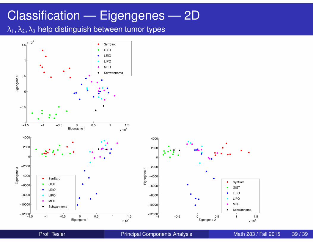
Classification — Eigengenes — 2Dλ1, λ2, λ3 help distinguish between tumor types

!!"# !! !$"# $ $"# ! !"#%&!$'

!!

!$"#

$

$"#

!

!"# %&!$'

()*+,*+,+&!

()*+,*+,+&-

./,.01234.56(4764879:;.2<=0,,>?0

!!"# !! !$"# $ $"# ! !"#%&!$'

!!($$$

!!$$$$

!)$$$

!*$$$

!'$$$

!($$$

$

($$$

'$$$

+,-./-./.&!

+,-./-./.&0

12/134567189+7:97;:<=>15?@3//AB3

!! !"#$ " "#$ ! !#$%&!"'

!!("""

!!""""

!)"""

!*"""

!'"""

!("""

"

("""

'"""

+,-./-./.&(

+,-./-./.&0

12/134567189+7:97;:<=>15?@3//AB3


Documents

Fall 2015 Math 283 Prof. Teslergptesler/283/slides/pca_15-handout.pdf · 31.9702 -16.5683-16.5683 13.0018 = s XX s XY s YX s ... Prof. Tesler Principal Components Analysis Math 283