arX

iv:c

s/06

1012

2v1

[cs

.NA

] 2

0 O

ct 2

006

Faithful Polynomial Evaluation

with Compensated Horner Algorithm

Philippe Langlois, Nicolas LouvetUniversite de Perpignan Via Domitia∗

{langlois, nlouvet}@univ-perp.fr

October 31, 2018

Abstract

This paper presents two sufficient conditions to ensure a faithful evaluation of

polynomial in IEEE-754 floating point arithmetic. Faithfulness means that the

computed value is one of the two floating point neighbours of the exact result; it

can be satisfied using a more accurate algorithm than the classic Horner scheme.

One condition here provided is an a priori bound of the polynomial condition

number derived from the error analysis of the compensated Horner algorithm. The

second condition is both dynamic and validated to check at the running time the

faithfulness of a given evaluation. Numerical experiments illustrate the behavior of

these two conditions and that associated running time over-cost is really interesting.

Keywords: Polynomial evaluation, faithful rounding, Horner algorithm, compen-sated Horner algorithm, floating point arithmetic, IEEE-754 standard.

1 Introduction

1.1 Motivation

Horner’s rule is the classic algorithm when evaluating a polynomial p(x). When performedin floating point arithmetic this algorithm may suffer from (catastrophic) cancellationsand so yields a computed value with less exact digits than expected. The relative accuracyof the computed value p(x) verifies the well known following inequality,

|p(x)− p(x)|

|p(x)|≤ α(n) cond(p, x) u. (1)

In the right-hand side of this accuracy bound, u is the computing precision andα(n) ≈ 2n for a polynomial of degree n. The condition number cond(p, x) that onlydepends on x and on p coefficients will be explicited further. The product α(n) cond(p, x)may be arbitrarily larger than 1/u when cancellations appear, i.e., when evaluating thepolynomial p at the x entry is ill-conditioned.

∗DALI Research Team. Laboratory LP2A. 52, avenue Paul Alduy. F-66860 Perpignan, France.

1

When the computing precision u is not sufficient to guarantee a desired accuracy,several solutions simulating a computation with more bits exist. Priest-like “double-double” algorithms are well-known and well-used solutions to simulate twice the IEEE-754 double precision [9, 7]. The compensated Horner algorithm is a fast alternative to“double-double” introduced in [2] — fast means that the compensated algorithm shouldrun at least twice as fast as the “double-double” counterpart with the same outputaccuracy. In both cases this accuracy is improved and now verifies

|p(x)− p(x)|

|p(x)|≤ u+ β(n) cond(p, x) u2, (2)

with β(n) ≈ 4n2. This relation means that the computed value is as accurate as theresult of the Horner algorithm performed in twice the working precision and thenrounded to this working precision.

This bound also tells us that such algorithms may yield a full precision accuracy fornot too ill-conditioned polynomials, e.g., when β(n) cond(p, x)u < 1.

This remark motivates this paper where we consider faithful polynomial evaluation.By faithful (rounding) we mean that the computed result p(x) is one of the two floatingpoint neighbours of the exact result p(x). Faithful rounding is known to be an interestingproperty since for example it guarantees the correct sign determination of arithmeticexpressions, e.g., for geometric predicates.

We first provide an a priori sufficient criterion on the condition number of the poly-nomial evaluation to ensure that the compensated Horner algorithm provides a faithfulrounding of the exact evaluation (Theorem 7 in Section 3). We also propose a validatedand dynamic bound to prove at the running time that the computed evaluation is ac-tually faithful (Theorem 9 in Section 4). We present numerical experiments to showthat the dynamic bound is sharper than the a priori condition and we measure that thecorresponding over-cost is reasonable (Section 5).

1.2 Notations

Throughout the paper, we assume a floating point arithmetic adhering to the IEEE-754floating point standard [5]. We constraint all the computations to be performed in oneworking precision, with the “round to the nearest” rounding mode. We also assume thatno overflow nor underflow occurs during the computations. Next notations are standard(see [4, chap. 2] for example). F is the set of all normalized floating point numbers and udenotes the unit roundoff, that is half the spacing between 1 and the next representablefloating point value. For IEEE-754 double precision with rounding to the nearest, wehave u = 2−53 ≈ 1.11 · 10−16. We define the floating point predecessor and successor of areal number r as follows,

pred(r) = max{f ∈ F/f < r} and succ(r) = min{f ∈ F/r < f}.

A floating point number f is defined to be a faithful rounding of a real number r if

pred(f) < r < succ(f).

2

The symbols ⊕, ⊖, ⊗ and⊘ represent respectively the floating point addition, subtrac-tion, multiplication and division. For more complex arithmetic expressions, fl(·) denotesthe result of a floating point computation where every operation inside the parenthesis isperformed in the working precision. So we have for example, a⊕ b = fl(a + b).

When no underflow nor overflow occurs, the following standard model describes theaccuracy of every considered floating point computation. For two floating point numbersa and b and for ◦ in {+,−,×, /}, the floating point evaluation fl(a ◦ b) of a ◦ b is suchthat

fl(a ◦ b) = (a ◦ b)(1 + ε1) = (a ◦ b)/(1 + ε2),with |ε1|, |ε2| ≤ u. (3)

To keep track of the (1 + ε) factors in next error analysis, we use the classic (1 + θk)and γk notations [4, chap. 3]. For any positive integer k, θk denotes a quantity boundedaccording to

|θk| ≤ γk =ku

1− ku.

When using these notations, we always implicitly assume ku < 1. In further erroranalysis, we essentially use the following relations,

(1 + θk)(1 + θj) ≤ (1 + θk+j), ku ≤ γk, γk ≤ γk+1.

Next bounds are computable floating point values that will be useful to derive dynamicvalidation in Section 4. We denotes fl(γk) = (ku) ⊘ (1 ⊖ ku) by γk. We know thatfl(ku) = ku ∈ F, and ku < 1 implies fl(1− ku) = 1− ku ∈ F. So γk only suffers from arounding error in the division and

γk ≤ (1 + u) γk. (4)

The next bound comes from the direct application of Relation (3). For x ∈ F and n ∈ N,

(1 + u)n|x| ≤ fl

(|x|

1− (n + 1)u

). (5)

2 From Horner to compensated Horner algorithm

The compensated Horner algorithm improves the classic Horner iteration computing acorrecting term to compensate the rounding errors the classic Horner iteration gener-ates in floating point arithmetic. Main results about compensated Horner algorithm aresummarized in this section; see [2] for a complete description.

2.1 Polynomial evaluation and Horner algorithm

The classic condition number of the evaluation of p(x) =∑n

i=0aix

i at a given data x is

cond(p, x) =

∑n

i=0|ai||x|

i

|∑n

i=0aixi|

=p(x)

|p(x)|. (6)

For any floating point value x we denote by Horner (p, x) the result of the floating pointevaluation of the polynomial p at x using next classic Horner algorithm.

3

Algorithm 1. Horner algorithm

function r0 = Horner (p, x)rn = anfor i = n− 1 : −1 : 0ri = ri+1 ⊗ x⊕ ai

end

The accuracy of the result of Algorithm 1 verifies introductory inequality (1) withαnu = γ2n and previous condition number (6). Clearly, the condition number cond(p, x)can be arbitrarily large. In particular, when cond(p, x) > 1/γ2n, we cannot guaranteethat the computed result Horner (p, x) contains any correct digit.

We further prove that the error generated by the Horner algorithm is exactly the sumof two polynomials with floating point coefficients. The next lemma gives bounds of thegenerated error when evaluating this sum of polynomials applying the Horner algorithm.

Lemma 1. Let p and q be two polynomials with floating point coefficients, such thatp(x) =

∑n

i=0aix

i and q(x) =∑n

i=0bix

i. We consider the floating point evaluation of (p+q)(x) computed with Horner (p⊕ q, x). Then, in case no underflow occurs, the computedresult satisfies the following forward error bound,

|(p+ q)(x)− Horner (p⊕ q, x) | ≤ γ2n+1( p+ q)(x). (7)

Moreover, if we assume that x and the coefficients of p and q are non-negative floatingpoint numbers then

(p+ q)(x) ≤ (1 + u)2n+1Horner (p⊕ q, x) . (8)

Proof. The proof of the error bound (7) is easily adapted from the one of the Horneralgorithm (see [4, p.95] for example). To prove (8) we consider Algorithm 1, where

rn = an ⊕ bn and ri = ri+1 ⊗ x⊕ (ai ⊕ bi) for i = n− 1, . . . , 0.

Next, using the standard model (3) it is easily proved by induction that, for i = 0, . . . , n,

i∑

j=0

(an−i+j + bn−i+j)xj ≤ (1 + u)2i+1rn−i, (9)

which in turn proves (8) for i = n.

2.2 EFT for the elementary operations

Now we review well known results concerning error free transformation (EFT) of theelementary floating point operations +, − and ×.

Let ◦ be an operator in {+,−,×}, a and b be two floating point numbers, and x =fl(a ◦ b). Then their exist a floating point value y such that

a ◦ b = x+ y. (10)

4

The difference y between the exact result and the computed result is the rounding errorgenerated by the computation of x. Let us emphasize that relation (10) between fourfloating point values relies on real operators and exact equality, i.e., not on approximatefloating point counterparts. Ogita et al. [8] name such a transformation an error freetransformation (EFT). The practical interest of the EFT comes from next Algorithms 2and 4 that compute the exact error term y for ◦ = + and ◦ = ×.

For the EFT of the addition we use Algorithm 2, the well known TwoSum algorithmby Knuth [6] that requires 6 flop (floating point operations). For the EFT of the product,we first need to split the input arguments into two parts. It is done using Algorithm 3 ofDekker [1] where r = 27 for IEEE-754 double precision. Next, Algorithm 4 by Veltkamp(see [1]) can be used for the EFT of the product. This algorithm is commonly calledTwoProd and requires 17 flop.

Algorithm 2. EFT of the sum of two floating point numbers.

function [x, y] = TwoSum (a, b)x = a⊕ bz = x⊖ ay = (a⊖ (x⊖ z))⊕ (b⊖ z)

Algorithm 3. Splitting of a floating point number into two parts.

function [x, y] = Split (a)z = a⊗ (2r + 1)x = z ⊖ (z ⊖ a)y = a⊖ x

Algorithm 4. EFT of the product of two floating point numbers.

function [x, y] = TwoProd (a, b)x = a⊗ b[ah, al] = Split (a)[bh, bl] = Split (b)y = al ⊗ bl ⊖ (((x⊖ ah ⊗ bh)⊖ al ⊗ bh)⊖ ah ⊗ bl)

The next theorem exhibits the previously announced properties of TwoSum andTwoProd.

Theorem 2 ([8]). Let a, b in F and x, y ∈ F such that [x, y] = TwoSum(a, b) (Algorithm2). Then, ever in the presence of underflow,

a+ b = x+ y, x = a⊕ b, |y| ≤ u|x|, |y| ≤ u|a + b|.

Let a, b ∈ F and x, y ∈ F such that [x, y] = TwoProd(a, b) (Algorithm 4). Then, if nounderflow occurs,

a× b = x+ y, x = a⊗ b, |y| ≤ u|x|, |y| ≤ u|a× b|.

5

We notice that algorithms TwoSum and TwoProd only require well optimizable floatingpoint operations. They do not use branches, nor access to the mantissa that can be time-consuming. We just mention that significant improvements of these algorithms are definedwhen a Fused-Multiply-and-Add operator is available [2].

2.3 An EFT for the Horner algorithm

As previously mentioned, next EFT for the polynomial evaluation with the Horner algo-rithm exhibits the exact rounding error generated by the Horner algorithm together withan algorithm to compute it.

Algorithm 5. EFT for the Horner algorithm

function [s0, pπ, pσ] = EFTHorner(p, x)sn = anfor i = n− 1 : −1 : 0[pi, πi] = TwoProd(si+1, x)[si, σi] = TwoSum(pi, ai)Let πi be the coefficient of degree i in pπLet σi be the coefficient of degree i in pσ

end

Theorem 3 ([2]). Let p(x) =∑n

i=0aix

i be a polynomial of degree n with floating pointcoefficients, and let x be a floating point value. Then Algorithm 5 computes both

i) the floating point evaluation Horner (p, x) and

ii) two polynomials pπ and pσ of degree n− 1 with floating point coefficients,

such that[Horner (p, x) , pπ, pσ] = EFTHorner (p, x) .

If no underflow occurs,

p(x) = Horner (p, x) + (pπ + pσ)(x). (11)

Moreover,( pπ + pσ)(x) ≤ γ2n p(x). (12)

Relation (11) means that algorithm EFTHorner is an EFT for polynomial evaluationwith the Horner algorithm.

Proof of Theorem 3. Since TwoProd and TwoSum are EFT from Theorem 2 it followsthat si+1x = pi + πi and pi + ai = si + σi. Thus we have si = si+1x + ai − πi − σi, fori = 0, . . . , n− 1. Since sn = an, at the end of the loop we have

s0 =n∑

i=0

aixi −

n−1∑

i=0

πixi −

n−1∑

i=0

σixi,

which proves (11).

6

Now we prove relation (12) According to the error analysis of the Horner algorithm(see [4, p.95]), we can write

Horner (p, x) = (1 + θ2n)anxn +

n−1∑

i=0

(1 + θ2i+1)aixi,

where every θk satisfies |θk| ≤ γk. Then using (11) we have

(pπ + pσ)(x) = p(x)− Horner (p, x) = −θ2nanxn −

n−1∑

i=0

θ2i+1aixi.

Therefore it yields next expected inequalities between the absolute values,

( pπ + pσ)(x) ≤ γ2n|an||x|n +

n−1∑

i=0

γ2i+1|ai||x|i ≤ γ2n p(x).

2.4 Compensated Horner algorithm

From Theorem 3 the final forward error of the floating point evaluation of p at x accordingto the Horner algorithm is

c = p(x)− Horner (p, x) = (pπ + pσ)(x),

where the two polynomials pπ and pσ are exactly identified by EFTHorner (Algorithm 5)—this latter also computes Horner (p, x). Therefore, the key of the compensated algorithmis to compute, in the working precision, first an approximate c of the final error c andthen a corrected result

r = Horner (p, x)⊕ c.

These two computations leads to next compensated Horner algorithm CompHorner (Al-gorithm 6).

Algorithm 6. Compensated Horner algorithm

function r = CompHorner (p, x)[ r, pπ, pσ] = EFTHorner (p, x)c = Horner (pπ ⊕ pσ, x)r = r ⊕ c

We say that c is a correcting term for Horner (p, x). The corrected result r is expectedto be more accurate than the first result Horner (p, x) as proved in next section.

3 An a priori condition for faithful rounding

We start proving the accuracy behavior of the compensated Horner algorithm we pre-viously mentioned with introductory inequality (2) and that motivates the search for afaithful polynomial evaluation. This bound (and its proof) is the first step towards theproposed a priori sufficient condition for a faithful rounding with compensated Horneralgorithm.

7

3.1 Accuracy of the compensated Horner algorithm

Next result proves that the result of a polynomial evaluation computed with the compen-sated Horner algorithm (Algorithm 6) is as accurate as if computed by the classic Horneralgorithm using twice the working precision and then rounded to the working precision.

Theorem 4 ([2]). Consider a polynomial p of degree n with floating point coefficients,and x a floating point value. If no underflow occurs,

|CompHorner (p, x)− p(x)| ≤ u|p(x)| + γ2

2n p(x). (13)

Proof. The absolute forward error generated by Algorithm 6 is

| r − p(x)| = |( r ⊕ c)− p(x)| = |(1 + ε)( r + c)− p(x)| with |ε| ≤ u.

Let c = (pπ + pσ)(x). From Theorem 3 we have r = Horner (p, x) = p(x)− c, thus

| r − p(x)| = |(1 + ε) (p(x)− c+ c)− p(x)| ≤ u|p(x)|+ (1 + u)| c− c|.

Since c = Horner (pπ ⊕ pσ, x) with pπ and pσ two polynomials of degree n− 1, Lemma 1

yields | c − c| ≤ γ2n−1( pπ + pσ)(x). Then using (12) we have | c − c| ≤ γ2n−1γ2n p(x).Since (1 + u)γ2n−1 ≤ γ2n, we finally write the expected error bound (13).

Remark 1. For later use, we notice that | c− c| ≤ γ2n−1γ2n p(x) implies

| c− c| ≤ γ2

2n p(x). (14)

It is interesting to interpret the previous theorem in terms of the condition numberof the polynomial evaluation of p at x. Combining the error bound (13) with the con-dition number (6) of polynomial evaluation gives the precise writing of our introductoryinequality (2),

|CompHorner (p, x)− p(x)|

|p(x)|≤ u+ γ2

2n cond(p, x). (15)

In other words, the bound for the relative error of the computed result is essentially γ22n

times the condition number of the polynomial evaluation, plus the inevitable summandu for rounding the result to the working precision. In particular, if cond(p, x) < u/γ2

2n,then the relative accuracy of the result is bounded by a constant of the order u. Thismeans that the compensated Horner algorithm computes an evaluation accurate to thelast few bits as long as the condition number is smaller than u/γ2

2n ≈ 1/4n2u. Besidesthat, relation (15) tells us that the computed result is as accurate as if computed bythe classic Horner algorithm with twice the working precision, and then rounded to theworking precision.

3.2 An a priori condition for faithful rounding

Now we propose a sufficient condition on cond(p, x) to ensure that the corrected resultr computed with the compensated Horner algorithm is a faithful rounding of the exactresult p(x). For this purpose, we use the following lemma from [10].

8

Lemma 5 ([10]). Let r, δ be two real numbers and r = fl(r). We assume here that r isa normalized floating point number. If |δ| < u

2| r| then r is a faithful rounding of r + δ.

From Lemma 5, we derive a useful criterion to ensure that the compensated resultprovided by CompHorner is faithfully rounded to the working precision.

Lemma 6. Let p be a polynomial of degree n with floating point coefficients, andx be a floating point value. We consider the approximate r of p(x) computed withCompHorner (p, x), and we assume that no underflow occurs during the computation. Letc denotes c = (pπ + pσ)(x). If | c− c| < u

2| r|, then r is a faithful rounding of p(x).

Proof. We assume that | c − c| < u

2| r|. From the notations of Algorithm 6, we recall

that fl( r + c) = r. Then from Lemma 5 it follows that r is a faithful rounding ofr+ c+ c− c = r+ c. Since [ r, pπ, pσ] = EFTHorner (p, x), Theorem 3 yields p(x) = r+ c.Therefore r is a faithful rounding of p(x).

The criterion proposed in Lemma 6 concerns the accuracy of the correcting term c.Nevertheless Relation (14) pointed after the proof of Theorem 4 says that the absoluteerror | c − c| is bounded by γ2

2n p(x). This provides us a more useful criterion, sinceit relies on the condition number cond(p, x), to ensure that CompHorner computes afaithfully rounded result.

Theorem 7. Let p be a polynomial of degree n with floating point coefficients, and x afloating point value. If

cond(p, x) <1− u

2 + uuγ2n

−2, (16)

then CompHorner (p, x) computes a faithful rounding of the exact p(x).

Proof. We assume that (16) is satisfied and we use the same notations as in Lemma 6.First we notice that r and p(x) are of the same sign. Indeed, from (13) it follows

that | r/p(x)− 1| ≤ u + γ22n cond(p, x), and therefore r/p(x) ≥ 1 − u − γ2

2n cond(p, x).But (16) implies that 1 − u − γ2

2n cond(p, x) > 1 − 3u/(2 + u) > 0, hence r/p(x) > 0.Since r and p(x) have the same sign, it is easy to see that

(1− u)|p(x)| − γ2

2n p(x) ≤ | r|. (17)

Indeed, if p(x) > 0 then (13) implies p(x) − u|p(x)| − γ22n p(x) ≤ r = | r|. If p(x) < 0,

from (13) it follows that r ≤ p(x)+u|p(x)|+γ22n p(x), hence −p(x)−u|p(x)|−γ2

2n p(x) ≤− r = | r|.

Next, a small computation proves that

cond(p, x) <1− u

2 + uuγ2n

−2 if and only if γ2

2n p(x) <u

2

[(1− u)|p(x)| − γ2

2n p(x)].

Finally, from (14) and (17) it follows

| c− c| ≤ γ2

2n p(x) <u

2

[(1− u)|p(x)| − γ2

2n p(x)]≤

u

2| r|.

From Lemma 6 we deduce that r is a faithful rounding of p(x).

Numerical values of condition numbers for a faithful polynomial evaluation in IEEE-754 double precision are presented in Table 1 for degrees varying from 10 to 500.

9

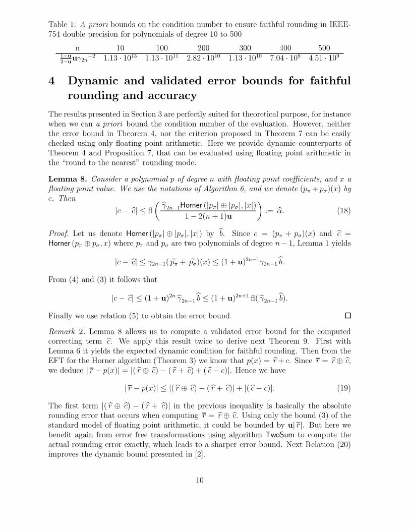
Table 1: A priori bounds on the condition number to ensure faithful rounding in IEEE-754 double precision for polynomials of degree 10 to 500

n 10 100 200 300 400 5001−u

2−uuγ2n

−2 1.13 · 1013 1.13 · 1011 2.82 · 1010 1.13 · 1010 7.04 · 109 4.51 · 109

4 Dynamic and validated error bounds for faithful

rounding and accuracy

The results presented in Section 3 are perfectly suited for theoretical purpose, for instancewhen we can a priori bound the condition number of the evaluation. However, neitherthe error bound in Theorem 4, nor the criterion proposed in Theorem 7 can be easilychecked using only floating point arithmetic. Here we provide dynamic counterparts ofTheorem 4 and Proposition 7, that can be evaluated using floating point arithmetic inthe “round to the nearest” rounding mode.

Lemma 8. Consider a polynomial p of degree n with floating point coefficients, and x afloating point value. We use the notations of Algorithm 6, and we denote (pπ + pσ)(x) byc. Then

|c− c| ≤ fl

(γ2n−1Horner (|pπ| ⊕ |pσ|, |x|)

1− 2(n+ 1)u

):= α. (18)

Proof. Let us denote Horner (|pπ| ⊕ |pσ|, |x|) by b. Since c = (pπ + pσ)(x) and c =Horner (pπ ⊕ pσ, x) where pπ and pσ are two polynomials of degree n− 1, Lemma 1 yields

|c− c| ≤ γ2n−1( pπ + pσ)(x) ≤ (1 + u)2n−1γ2n−1 b.

From (4) and (3) it follows that

|c− c| ≤ (1 + u)2n γ2n−1 b ≤ (1 + u)2n+1 fl( γ2n−1 b).

Finally we use relation (5) to obtain the error bound.

Remark 2. Lemma 8 allows us to compute a validated error bound for the computedcorrecting term c. We apply this result twice to derive next Theorem 9. First withLemma 6 it yields the expected dynamic condition for faithful rounding. Then from theEFT for the Horner algorithm (Theorem 3) we know that p(x) = r+ c. Since r = r⊕ c,we deduce | r − p(x)| = |( r ⊕ c)− ( r + c) + ( c− c)|. Hence we have

| r − p(x)| ≤ |( r ⊕ c)− ( r + c)|+ |( c− c)|. (19)

The first term |( r ⊕ c) − ( r + c)| in the previous inequality is basically the absoluterounding error that occurs when computing r = r ⊕ c. Using only the bound (3) of thestandard model of floating point arithmetic, it could be bounded by u| r|. But here webenefit again from error free transformations using algorithm TwoSum to compute theactual rounding error exactly, which leads to a sharper error bound. Next Relation (20)improves the dynamic bound presented in [2].

10

Theorem 9. Consider a polynomial p of degree n with floating point coefficients, and xa floating point value. Let r be the computed value, r = CompHorner (p, x) (Algorithm 6)and let α be the error bound defined by Relation (18).

i) If α < u

2| r|, then r is a faithful rounding of p(x) .

ii) Let e be the floating point value such that r+e = r+ c, i.e., [ r, e] = TwoSum ( r, c),where r and c are defined by Algorithm 6. The absolute error of the computed resultr = CompHorner (p, x) is bounded as follows,

| r − p(x)| ≤ fl

(α + |e|

1− 2u

):= β. (20)

Proof. The first proposition follows directly from Lemma 6.By hypothesis r = r + c− e, and from Theorem 3 we have p(x) = r + c, thus

| r − p(x)| = | c− c− e| ≤ | c− c|+ |e| ≤ α+ |e|.

From (3) and (5) it follows that

| r − p(x)| ≤ (1 + u) fl( α+ |e|) ≤ fl

(α + |e|

1− 2u

);

which proves the second proposition.

From Theorem 9 we deduce the following algorithm. It computes the compensatedresult r together with the validated error bound β. Moreover, the boolean value isfaithfulis set to true if and only if the result is proved to be faithfully rounded.

Algorithm 7. Compensated Horner algorithm with check of the faithful rounding

function [ r, β, isfaithful] = CompHornerIsFaithul (p, x)

[ r, pπ, pσ] = EFTHorner (p, x)

c = Horner (pπ ⊕ pσ, x)

b = Horner (|pπ| ⊕ |pσ|, |x|)

[ r, e] = TwoSum ( r, c)

α = ( γ2n−1 ⊗ b)⊘ (1⊖ 2(n+ 1)⊗ u)

β = ( α⊕ |e|)⊘ (1− 2⊗ u)

isfaithful = ( α < u

2| r|)

5 Experimental results

We consider polynomials p with floating point coefficients and floating point entries x. Forpresented accuracy tests we use Matlab codes for CompHorner (Algorithm 6) and Com-

pHornerIsFaithul (Algorithm 7). These Matlab programs are presented in Appendix 7.From these Matlab codes, we see that CompHorner requires O(21n) flop and that Com-

pHornerIsFaithul requires O(26n) flop.For time performance tests previous algorithms are coded in C language and several

test platforms are described in next Table 2.

11

Figure 1: We report the evaluation of polynomials pn near the multiple root x = 1 with thecompensated Horner algorithm (CompHornerIsFaithul) and for multiplicity n = 6, 8, 10, 12.Each evaluation proved to be faithfully rounded thanks to the dynamic test is reportedwith a green cross. The faithful evaluations that are not detected to be so with thedynamic test are represented in blue. Finally, the evaluations that are not faithfullyrounded are reported in red. The lower frame represents the condition number withrespect to the argument x.

5.1 Accuracy tests

We start testing the efficiency of faithful rounding with compensated Horner algorithmand the dynamic control of faithfulness. Then we focus more on both the a priori anddynamic bounds with two other test sets. Three cases may occur when the dynamic testfor faithful rounding in Algorithm 7 is performed.

1. The computed result is faithfully rounded and this is ensured by the dynamic test.Corresponding plots are green in next figures.

2. The computed result is actually faithfully rounded but the dynamic test fails toensure this property. Corresponding plots are blue.

3. The computed result is not faithfully rounded and plotted in red in this case.

Next figures should be observed in color.

5.1.1 Faithful rounding with compensated Horner

In the first experiment set, we evaluate the expanded form of polynomials pn(x) = (1−x)n,for degree n = 6, 8, 10, 12, at 2048 equally spaced floating point entries being near the

12

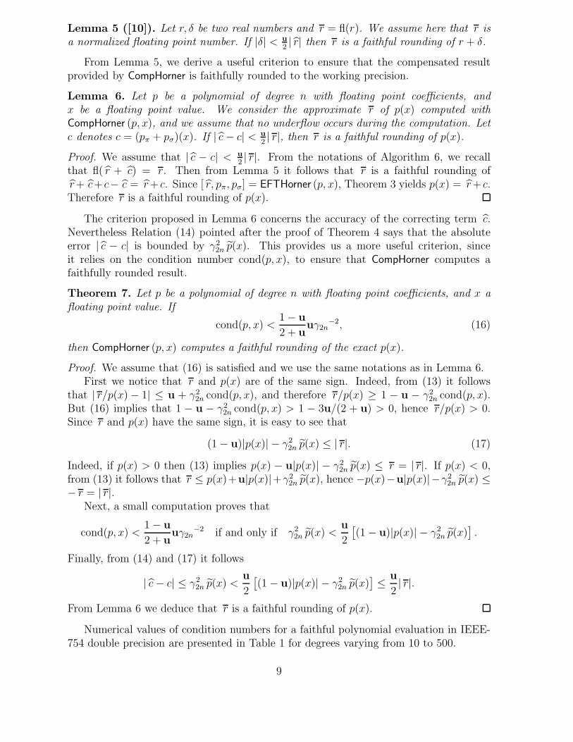
Figure 2: We report the relative accuracy of every polynomial evaluation (y axis) withrespect to the condition number (x axis). Evaluation is performed with CompHornerIs-

Faithul (Algorithm 7). The color code is the same as for Figure 1. Leftmost vertical line isthe a priori sufficient condition (16) while the right one marks the inverse of the workingprecision u. Broken line is the a priori accuracy bound (15).

multiple root x = 1. These evaluations are extremely ill-conditioned since

cond(pn, x) =

∣∣∣∣1 + |x|

1− x

∣∣∣∣n

.

These condition numbers are plotted in the lower frame of Figure 1 while x variesaround the root. These huge values have a sense since polynomials p are exact inIEEE-754 double precision. Results are reported on Figure 1. The well known relationbetween the lost of accuracy and the nearness and the multiplicity of the root, i.e., theincreasing of the condition number, is clearly illustrated. These results also illustratethat the dynamic bound becomes more pessimistic as the condition number increases.In next figures the horizontal axis does not represent the x entry range anymore but thecondition number which governs the whole behavior.

For the next experiment set, we first designed a generator of arbitrary ill-conditionedpolynomial evaluations. It relies on the condition number definition (6). Given a degree n,a floating point argument x and a targeted condition number C, it generates a polynomialp with floating point coefficients such that cond(p, x) has the same order of magnitudeas C. The principle of the generator is the following.

1. ⌊n/2⌋ coefficients are randomly selected and generated such that p(x) =∑|ai||x|

i ≈ C,

2. the remaining coefficients are generated ensuring |p(x)| ≈ 1 thanks to high accuracycomputation.

Therefore we obtain polynomials p such that cond(p, x) = p(x)/|p(x)| ≈ C, for arbitraryvalues of C.

13

Figure 3: The dynamic error bound (20) compared to the a priori bound (13) and to theactual forward error (p(x) = (1− x)5 for 400 entries on the x axis).

In this test set we consider generated polynomials of degree 50 whose condition num-bers vary from about 102 to 1035. These huge condition numbers again have a sense heresince the coefficients and the argument of every polynomial are floating point numbers.The results of the tests performed with CompHornerIsFaithul (Algorithm 7) are reportedon Figure 2. As expected every polynomial with a condition number smaller than the apriori bound (16) is faithfully evaluated with Algorithm 7 —green plots at the left of theleftmost vertical line.

On Figure 2 we also see that evaluations with faithful rounding appear for conditionnumbers larger than the a priori bound (16) — green and blue plots at the right ofthe leftmost vertical line. As expected a large part of these cases are detected by thedynamic test introduced in Theorem 9 —the green ones. Next experiment set comes backto this point. We also notice that the compensated Horner algorithm produces accurateevaluations for condition numbers up to about 1/u —green and blue plots.

5.1.2 Significance of the dynamic error bound

We illustrate the significance of the dynamic error bound (20), compared to the a priorierror bound (13) and to the actual forward error. We evaluate the expanded form ofp(x) = (1−x)5 for 400 points near x = 1. For each value of the argument x, we computeCompHorner (p, x) (Algorithm 6), the associated dynamic error bound (20) and the actualforward error. The results are reported on Figure 3.

As already noticed, the closer the argument is to the root 1 (i.e., , the more thecondition number increases), the more pessimistic becomes the a priori error bound.Nevertheless our dynamic error bound is more significant than the a priori error boundas it takes into account the rounding errors that occur during the computation.

14

Table 2: Measured time performances for CompHorner, CompHornerIsFaithul andDDHorner. GCC denotes the GNUCompiler Collection and ICC denotes the Intel C/C++Compiler.

CompHorner

Horner

CompHornerIsFaith

HornerDDHornerHorner

Pentium 4, 3.00 GHz GCC 3.3.5 3.77 5.52 10.00

ICC 9.1 3.06 5.31 8.88

Athlon 64, 2.00 GHz GCC 4.0.1 3.89 4.43 10.48

Itanium 2, 1.4 GHz GCC 3.4.6 3.64 4.59 5.50

ICC 9.1 1.87 2.30 8.78

∼ 2− 4 ∼ 4− 6 ∼ 5− 10

5.2 Time performances

All experiments are performed using IEEE-754 double precision. Since the double-doubles [3, 7] are usually considered as the most efficient portable library to double theIEEE-754 double precision, we consider it as a reference in the following comparisons.For our purpose, it suffices to know that a double-double number a is the pair (ah, al) ofIEEE-754 floating point numbers with a = ah+al and |al| ≤ u|ah|. This property impliesa renormalisation step after every arithmetic operation with double-double values. Wedenote by DDHorner our implementation of the Horner algorithm with the double-doubleformat, derived from the implementation proposed in [7].

We implement the three algorithms CompHorner, CompHornerIsFaith and DDHorner

in a C code to measure their overhead compared to the Horner algorithm. We programthese tests straightforwardly with no other optimization than the ones performed by thecompiler. All timings are done with the cache warmed to minimize the memory trafficover-cost.

We test the running times of these algorithms for different architectures with differentcompilers as described in Table 2. Our measures are performed with polynomials whosedegree vary from 5 to 200 by step of 5. For each algorithm, we measure the ratio of itscomputing time over the computing time of the classic Horner algorithm; we display theaverage time ratio over all test cases in Table 2.

The results presented in Table 2 show that the slowdown factor introduced by Com-

pHorner compared to the classic Horner roughly varies between 2 and 4. The same slow-down factor varies between 4 and 6 for CompHornerIsFaithul and between 5 and 10 forDDHorner. We can see that CompHornerIsFaithul runs a most 2 times slower than Com-

pHorner: the over-cost due to the dynamic test for faithful rounding is therefore quitereasonable. Anyway CompHorner and CompHornerIsFaithul run both significantly fasterthan DDHorner.

Remark 3. We provide time ratios for IA’64 architecture (Itanium 2). Tested algorithmstake benefit from IA’64 instructions, e.g., fma, but are not described in this paper.

15

6 Conclusion

Compensated Horner algorithm yields more accurate polynomial evaluation than the clas-sic Horner iteration. Its accuracy behavior is similar to an Horner iteration performed ina doubled working precision. Hence compensated Horner may perform a faithful poly-nomial evaluation with IEEE-754 floating point arithmetic in the “round to the nearest”rounding mode. An a priori sufficient condition with respect on the condition numberthat ensures such faithfulness has been defined thanks to the error free transformations.

These error free transformations also allow us to derive a dynamic sufficient conditionthat is more significant to check for faithful rounding with compensated Horner algorithm.

It is interesting to remark here that the significance of this dynamic bound can beimproved easily —how to transform blue plots in green ones? Whereas bounding theerror in the computation of the (polynomial) correcting term in Relation (18), a goodapproximate of the actual error could be computed (applying again CompHorner to thecorrecting term). Of course such extra computation will introduce more running timeoverhead not necessary useful —green plots are here! So it suffices to run such extra (butcostly) checking only if the previous dynamic one fails (a similar strategy as in dynamicfilters for geometric algorithms).

Compared to the classic Horner algorithm, experimental results exhibit reasonableover-costs for accurate polynomial evaluation (between 2 and 4) and even for this com-putation with a dynamic checking for faithfulness (between 4 and 6). Let us finallyremark than such computation that provides as accuracy as if the working precision isdoubled and a faithfulness checking is no more costly in term of running time than the“double-double” counterpart without any check.

Future work will be to consider subnormals results and also an adaptative algorithmthat ensure faithful rounding for polynomials with an arbitrary condition number.

References

[1] T. J. Dekker. A floating-point technique for extending the available precision. Numer.Math., 18:224–242, 1971.

[2] S. Graillat, P. Langlois, and N. Louvet. Compensated Horner scheme. Technicalreport, University of Perpignan, France, July 2005.

[3] Y. Hida, X. S. Li, and D. H. Bailey. Algorithms for quad-double precision floatingpoint arithmetic. In N. Burgess and L. Ciminiera, editors, Proceedings of the 15thSymposium on Computer Arithmetic, Vail, Colorado, pages 155–162, Los Alamitos,CA, USA, 2001. Institute of Electrical and Electronics Engineers.

[4] N. J. Higham. Accuracy and Stability of Numerical Algorithms. Society for Industrialand Applied Mathematics, Philadelphia, PA, USA, second edition, 2002.

[5] IEEE Standards Committee 754. IEEE Standard for binary floating-point arithmetic,ANSI/IEEE Standard 754-1985. Institute of Electrical and Electronics Engineers,Los Alamitos, CA, USA, 1985. Reprinted in SIGPLAN Notices, 22(2):9-25, 1987.

16

[6] D. E. Knuth. The Art of Computer Programming: Seminumerical Algorithms, vol-ume 2. Addison-Wesley, Reading, MA, USA, third edition, 1998.

[7] X. S. Li, J. W. Demmel, D. H. Bailey, G. Henry, Y. Hida, J. Iskandar, W. Kahan,S. Y. Kang, A. Kapur, M. C. Martin, B. J. Thompson, T. Tung, and D. J. Yoo.Design, implementation and testing of extended and mixed precision BLAS. ACMTrans. Math. Software, 28(2):152–205, 2002.

[8] T. Ogita, S. M. Rump, and S. Oishi. Accurate sum and dot product. SIAM J. Sci.Comput., 26(6):1955–1988, 2005.

[9] D. M. Priest. Algorithms for arbitrary precision floating point arithmetic. In P. Ko-rnerup and D. W. Matula, editors, Proceedings of the 10th IEEE Symposium onComputer Arithmetic (Arith-10),Grenoble, France, pages 132–144, Los Alamitos,CA, USA, 1991. Institute of Electrical and Electronics Engineers.

[10] S. M. Rump, T. Ogita, and S. Oishi. Accurate summation. Technical report, Ham-burg University of Technology, Germany, Nov. 2005.

7 Appendix

Accuracy tests use next Matlab codes for algorithms Algorithm 6 (CompHorner) andAlgorithm 7 (CompHornerIsFaithul). Following Matlab convention, p is represented as avector p such that p(x) =

∑n

i=0p(n − i + 1)xi. We also recall that Matlab eps denotes

the machine epsilon, which is the spacing between 1 and the next larger floating pointnumber, hence u = eps/2.

17

Algorithm 8. Code for Algorithm 6.

function r = CompHorner(p, x)n = length(p)-1; % degree of p[xh, xl] = Split(x);r = p(1); c = 0.0;for i=2:n+1%[r, pi] = TwoProd(r, x)p = r*x;[rh, rl] = Split(r);pi = rl*xl-(((p-rh*xl)-rl*xh)-rh*xl);%[r, sigma] = TwoSum(r, p(i))r = p+p(i);t = r-p;sigma = (p-(r-t))+(p(i)-t);% Computation of the correcting termc = c*x+(pi+sig);

end% Final correction of the resultr = r+c;

Algorithm 9. Code for Algorithm 7.

function [r, beta, isfaith] = CompHornerIsFaithul(p, x)n = length(p)-1; % degree of p[xh, xl] = Split(x);absx = abs(x);r = p(1); c = 0.0; beta = 0.0;for i=2:n+1% [r, pi] = TwoProd(r, x)p = r*x;% [rh, rl] = Split(r);pi = rl*xl-(((p-rh*xl)-rl*xh)-rh*xl);% [r, sigma] = TwoSum(r, p(i))r = p+p(i);t = r-p;sigma = (p-(r-t))+(p(i)-t);% Computation of the correcting termc = c*x+(pi+sig);b = b*absx+(abs(pi)+ abs(sig));

end% Final correction of the result[r, e] = TwoSum(r,c);% Check for faithful roundingalpha = gam(2*n-1)*b / (1-(n+1)*eps);isfaith = alpha ¡ 0.25*eps*abs(r);% Absolute error boundbeta = (alpha + abs(e))/(1-2*u);

18