NOVEMBER 2000 GMU/C3I-230-TH

PERFORMANCE PREDICTION OF REAL -TIME

COMMAND, CONTROL, AND COMMUNICATIONS

(C3) SYSTEMS

By

Insub Shin

DISTRIBUTION STATEMENT A Approved for Public Release

Distribution Unlimited

System Architectures Laboratory Center of Excellence in Command, Control, Communications, and Intelligence (C3I)

George Mason University Fairfax, Virginia 22030

20010712 005

REPORT DOCUMENTATION PAGE Public reporting burden for this collection of information is estimated to average 1 hour per response, including the time for reviewing ii AFRL-SR-BL-TR-01 ■ data needed, and completing and reviewing this collection of information. Send comments regarding this burden estimate or any other this burden to Department of Defense, Washington Headquarters Services, Directorate for Information Operations and Reports (0704-' 4302. Respondents should be aware that notwithstanding any other provision of law, no person shall be subject to any penalty for faili valid OMB control number. PLEASE DO NOT RETURN YOUR FORM TO THE ABOVE ADDRESS. o^'&Sr'

gthe icing 12- rently

1. REPORT DATE (DD-MM-YYYY) 31-10-2000

2. REPORT TYPE Final Technical Report

4. TITLE AND SUBTITLE Performance Prediction of Real-Time Command, Control,

Communications (C3) Systems

and

Nov 1998 - Oct 2000 5a. CONTRACT NUMBER

6. AUTHOR(S)

Shin, Insub and Levis, Alexander H.

7. PERFORMING ORGANIZATION NAME(S) AND ADDRESS(ES)

System Architectures Lab. C3I Center George Mason University Fairfax, VA 22030

5b. GRANT NUMBER F49620-98-1-0179 5c. PROGRAM ELEMENT NUMBER

5d. PROJECT NUMBER

5e. TASK NUMBER

5f. WORK UNIT NUMBER

9. SPONSORING / MONITORING AGENCY NAME(S) AND ADDRESS(ES) Air Force Office for

Scientific Research 810 N. Randolph Street Arlington, VA 22203-1977

12. DISTRIBUTION / AVAILABILITY STATEMENT

Distribution Unlimited

8. PERFORMING ORGANIZATION REPORT NUMBER

GMU/C3I/SAL-230-TH

10. SPONSOR/MONITOR'S ACRONYM(S) AFOSR

11. SPONSOR/MONITOR'S REPORT NUMBER(S)

sssssa 13. SUPPLEMENTARY NOTES füS^^^'8^0 ^P ^ APTOVCD FOfl PUBLIC HfcLfcAa,

14. ABSTRACT Predicting the performance of a C3 system consisting of sub-systems requires the integration of such sub-system models with the communication system models. When the system is used for a time critical mission, the network delay may play a decisive role in battle management. The architecture of a C3 system is represented by two layers: the functional layer and the physical layer. The synthetic execution model contains both architecture layers as separate executable models. Then, the layered executable models are combined to develop a performance prediction model. The executable functional model uses a Petri net to describe the logical behavior and the executable physical model uses a queuing net to represent the demand and/or contention of resources. The message-passing pattern is generated from the executable functional model using a state space analysis technique. The executable physical model processes these messages preserving the message-passing pattern. Once the network delay is measured in the executable physical model it is inserted into the functional model

15. SUBJECT TERMS |C3 Systems, Communication Models, Petri nets; Functional Architecture, Physical Architecture

116. SECURITY CLASSIFICATION OF: Unclassified

'a. REPORT uu

b. ABSTRACT UU

c. THIS PAGE UU

17. LIMITATION OF ABSTRACT

UU

18. NUMBER OF PAGES

vi + 170

I

19a. NAME OF RESPONSIBLE PERSON Alexander H. Levis 19b. TELEPHONE NUMBER (include area code)

703 993 1619

Standard Form 298 (Rev. 8-98) Prescribed by ANSI Std. Z39.18

October 2000 GMU/C3I/SAL-230-TH

PERFORMANCE PREDICTION OF REAL-TIME COMMAND, CONTROL, AND COMMUNICATIONS (C3) SYSTEMS

By

Insub Shin

This final technical report is based on the unaltered thesis of Insub Shin, submitted to the School of Information Technology and Engineering in partial fulfillment of the requirements for the degree of Doctor of Philosophy in Information Technology and Engineering at George Mason University in October 2000. The research was conducted at the System Architectures Laboratory of the C3I Center of George Mason University with support provided by the Air Force Office for Scientific Research under grant no. F49620-98-1-0179.

System Architectures Laboratory C3I Center

George Mason University Fairfax, VA 22030

PERFORMANCE PREDICTION OF REAL-TIME COMMAND, CONTROL, AND COMMUNICATIONS (C3) SYSTEMS

by

Insub Shin

ABSTRACT

Many of the Command, Control, and Communication (C3) systems in the real world are supported by a common network or a network of networks. Predicting the performance of a C3 system consisting of sub-systems requires the integration of such sub-system models with the communication system models. When the system is used for a time critical mission, the network delay may play a decisive role in battle management.

In this dissertation, the architecture of a C3 system is represented by two layers: the functional layer and the physical layer. The synthetic execution model contains both architecture layers as separate executable models. Then, the two layered executable models are combined to develop a performance prediction model.

The executable functional model uses a Petri net to describe the logical behavior and the executable physical model uses a queueing net to represent the demand and/or contention of resources. The message-passing pattern is generated from the executable functional model using a state space analysis technique. The executable physical model processes these messages preserving the message-passing pattern. Once the network delay is measured in the executable physical model, the delay value is inserted into the executable functional model for performance prediction.

Since the communication service demands are isolated from the executable functional model, the communications network can be specified in any preferred level of detail independently. This enables the executable functional model to be invariant with respect to the executable physical model resulting in flexibility for designing a large-scale C3 information system. This property, together with the synthesis technique, enables both formal and simulation methods to be used for system analysis: the state space analysis technique of Petri nets and the simulation technique of queueing nets.

A case study in this dissertation shows how a small network delay in a C3 system affects the outcome of a time critical mission. It also illustrates design choices and shows how to develop tactics to provide tolerance to network delays.

George Mason University Fairfax, Virginia

TABLE OF CONTENTS

1. INTRODUCTION 1

2. PROBLEM DEFINITION AND OBJECTIVES 11

3. THEORETICAL BACKGROUND 25

4. A METHODOLOGY TO DEVELOP SYNTHETIC EXECUTABLE MODELS 49

5. SYNTHETIC EXECUTABLE MODEL GENERATOR 73

6. A CASE STUDY 101

7. CONCLUSIONS 121

APPENDIX A: A computer implementation of colored Petri nets: Design/CPN 126

APPENDIX B: Description of the Petri net model of the AAW system 138

APPENDIX C: Performance measures for the AAW system 148

REFERENCES 165

in

LIST OF FIGURES

Figure 1.1 Integrated view of a System 3

Figure 1.2 Two Separate Functional and Physical Architecture Models 5

Figure 1.3 Run-Time Communication between Functional and Physical Architecture Models 6

Figure 1.4 Off-Line Communication between Functional and Physical Architecture Models 7

Figure 2.1 Operational Concept Diagram 11

Figure 2.2 Operational Sequence Diagram for AAW system 18

Figure 2.3 Measurement Issues for Performance Prediction of a Typical C3 System 19

Figure 2.4 Uncertainty vs. Time 21

Figure 2.5 Data Fusion Net 22

Figure 3.1 A Three-Phase System Architecting 25

Figure 3.2 Syntax of IDEFO Diagram 29

Figure 3.3 An Example of Architecture Specifications 29

Figure 3.4 An Example of a Pure Ordinary Petri net 33

Figure 3.5 Example of Markings of a Petri net 34

Figure 3.6 Firing of a Transition 35

Figure 3.7 Example of a Conflict net 35

Figure 3.8 Example of an Occurrence Graph 39

Figure 3.9 Execution of a Scalar Time in Distributed Execution 43

Figure 4.1 An Executable Functional Model as an Ordinary Petri net 49

IV

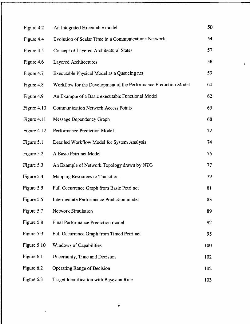
Figure 4.2 An Integrated Executable model 50

Figure 4.4 Evolution of Scalar Time in a Communications Network 54

Figure 4.5 Concept of Layered Architectural States 57

Figure 4.6 Layered Architectures 58 i

Figure 4.7 Executable Physical Model as a Queueing net 59

Figure 4.8 Workflow for the Development of the Performance Prediction Model 60

Figure 4.9 An Example of a Basic executable Functional Model 62

Figure 4.10 Communication Network Access Points 63

Figure 4.11 Message Dependency Graph 68

Figure 4.12 Performance Prediction Model 72

Figure 5.1 Detailed Workflow Model for System Analysis 74

Figure 5.2 A Basic Petri net Model 75

Figure 5.3 An Example of Network Topology drawn by NTG 77

Figure 5.4 Mapping Resources to Transition 79

Figure 5.5 Full Occurrence Graph from Basic Petri net 81

Figure 5.5 Intermediate Performance Prediction model 83

Figure 5.7 Network Simulation 89

Figure 5.8 Final Performance Prediction model 92

Figure 5.9 Full Occurrence Graph from Timed Petri net 95

Figure 5.10 Windows of Capabilities 100

Figure 6.1 Uncertainty, Time and Decision 102

Figure 6.2 Operating Range of Decision 102

Figure 6.3 Target Identification with Bayesian Rule

V

103

Figure 6.4 Target Tracking with Kaiman Filter 105

Figure 6.5 Command and Control of an Anti-Air Warfare System 106

Figure 6.6 Data Fusion for Target Identification 107

Figure 6.7 Data Fusion for Target Tracking 107

Figure 6.8 Command Decision 108

Figure 6.9 The Anti-Air Warfare System of the Example 109

Figure 6.10 Deployment Diagram of an AAW system 110

Figure 6.11 Top Level Diagram of an AAW system 114

Figure 6.12 Centralized Configuration of Multiple Sensors 116

Figure 6.13 Executable Physical Model 117

VI

CHAPTER 1. INTRODUCTION

1.1 Motivation

A Command, Control, and Communications (C3) system is typically a real-time distributed

system consisting of multiple software and multiple hardware components.

In general, a real time system is characterized by its timely response to external stimuli

(Tsai and Yang, 1995). A response consists of a series of task executions, and a task execution is

usually characterized by its start time, execution time, and deadline (Stankovic et al, 1985).

Analysis of the timing of each task and time management in a series of task executions are

essential to guarantee that the system responds at the right time, or before but not after a due

time.

A C3 system for a high-level military organization is a system-of-systems consisting of

heterogeneous subsystems in operation under distributed computing environments. At the early

stage of the system development cycle, however, there are significant uncertainties in the

performance parameters, task execution time, and communication delays. These uncertainties are

often due to incomplete system specifications and/or complexity of the problem. Furthermore,

the message delays from each subsystem can change the order of task execution in an

autonomous system and may cause a synchronization problem. Asynchronous execution at

distributed portions of the system may threaten the principles of military doctrine.

For a C3 system dealing with time critical missions, the estimates of the elapsed time for

each interacting subsystem and the message delay can play a critical role in developing combat

engagement rules, establishing decision thresholds, and battle time management. A well-formed

performance prediction model supported by an accurate timing estimate method is required.

1.2 Problem Statement

A number of researchers (Bucci et al.,1995; Li et al., 1998; Ostroff, 1989; Popova and

Heiner, 1997; Toussaint et al., 1997; Tsai et al., 1995) have addressed the verification of the

timing behavior, given timing constraints, instead of controlling the timing behavior of a real

1

time system. Timing constraints are expressed in the form of [tmin, tmax], where tmin and tmax are

the minimum and maximum time instants, respectively, elapsing between the enabling and

execution of each task. The execution of a task is constrained by external stimuli such as mission

requirements or by service capabilities of physical resources. The time interval can be interpreted

in various ways. Cothier (1984) used the notion of time interval as "timeliness" (called "window

of opportunity"). There are basically two types of windows: the window of capability which

characterizes the system response capabilities, while the window of opportunity expresses the

requirements of the mission which the system is expected to fulfill (Cothier, 1984). In terms of

the mission requirements involving a decision making process, the time interval represents the

windows of opportunity such that the decision must be made between tmin and tmax (after the

arrival of its input). In this case, tmax is an upper-bound threshold such that, if a decision making

organization issues commands in response to the input after the threshold, there will not be

enough time to execute the response (Andreadakis, 1988). A decision-making organization can

be seen as an information processing system that performs a series of tasks to accomplish its

mission (Andreadakis, 1988; Levis, 1991). In terms of a physical resource's performance

capability for information processing in the decision-making organization, the time interval

represents the windows of capability such that the information processing system is capable of

supporting the decision-making process only within that interval; the decision making

organization demands at least tmin time units and at most tmax time units to accomplish its decision

making process using the information processing system.

Setting different decision thresholds within the windows of opportunity may generate

different orderings of message passing among multiple tasks over a network. It may cause

different connection delays^ between tasks resulting in different windows of capability. In turn,

the different connection delays may cause different orderings of task executions and this may

violate task synchronization in an autonomous system without specific synchronization measure.

We encounter a "chicken and egg" problem. Thus, the performance prediction of a real-time

system derived under an assumption of communication delays with a probabilistic distribution

does not guarantee the realistic representation of the system's behavior unless we solve the

The term "connection delays" will be used in reference to the delay between two tasks in a functional architecture that is different from the data transmission delay between two nodes in a physical architecture.

"chicken and egg" problem. In the literature, the term "task" is sometimes used interchangeably

with "process," "grain," "thread," etc. (Dietz et al., 1997). In this report, the term "process" will

be used as an analogue to the term "task" when the task represents information processing. The

constraints of process synchronization include precedence constraints; a process, which produces

data for another process, will complete before that data is required, and exclusion constraints: if

either one of the two processes has started and is not yet finished, the other process cannot be

started (Dong et al., 1997). Delays over interconnections must be considered to manage the

complexity of meeting these synchronization constraints.

The properties and behavior of a system can be specified and expressed in various ways

depending on the point of view: decomposition into sub-systems or layering by architectural

levels. Predicting the performance of a real-time distributed system requires synthesis of the sub-

systems or layered architectures together with the communication network. The traditional

method is to represent the communication demand of each task and the contention of the

demands as an embedded link in a single integrated model. For example, Link^k+i) in Figure 1.1

is embedded in a single system.

Functional Laver

Information

Integrated view of a system

Information.

Physical Layer

Link (k,k+i)

Message. \ Node k+l

Figure 1.1 Integrated view of a System

This approach may have limitations in representing the demand and the contention of

network resources that are shared among multiple processes in a large-scale real-time distributed

system. The objective of this report is to present methods to synthesize architecture layers and to

estimate the connection delays between tasks so that the performance of a C3 system that

performs multiple tasks in a real-time distributed computing environment can be predicted.

1.3 Approach

Developing an executable model enables the prediction of the performance of a real time

system. Operational formalisms such as Petri nets (Murata,1989) and state machines are suitable

to specify and express executable models. For example, in a system architecting cycle of

analysis-synthesis-evaluation (Levis and Wagenhals, 2000), an executable model is developed

using a Petri net consisting of "transitions" and "places." Each "transition" and "place" can

represent tasks and resources respectively. Interactions between tasks are represented by "arcs".

The timing behavior of a system is derived by introducing time to either "transitions" or "places".

In the case of the Real-Time Object Oriented Modeling approach (Gullekson and Selic, 1996;

Selic, 1998), an executable model is represented by a network of collaborating state machines

called "actors" (i.e., software modules). Interactions between actors are represented by message-

passing through explicit interfaces called "ports". The receipt of a message by an actor triggers

the appropriate state transitions of the actor's state machine (its behavior). The timing behavior

of a system is handled by time-out events in its event-driven run-time "timing service". A task

can have as attribute "duration of time" (i.e., deadline or maximum processing time) and can

send a "time-out" event message to a timer at the desired instant when a task needs to initiate

time-related activity.

In both cases, we can model network delays between tasks as another "transition" or

"actor". If the physical communication link between tasks is simply an immediately adjacent

transmission link, the modeling effort may be easy. When multiple connections share common

network resources other than a single, immediate, adjacent transmission link, the cost of

modeling may be very high. In some cases, modeling the contention of communication resources

may be practically impossible. Also adding more "transitions" or "actors" can raise the problem

of state space explosion.

In this report, the logical behavior of a system is specified in a functional architecture layer

and the supporting resources are specified in a physical architecture layer. Both layers describe or

specify the same system. In the paradigm adopted in this report, each architecture layers are

modeled as a separate executable model and performance parameters are obtained by exchanging

the necessary state information between the two models.

Suppose that the two models are developed as shown in Figure 1.2 in which the functional

architecture model is a Petri net and the physical architecture model is a queueing net. The circle

in the functional architecture model is a "place" and the bar is a "transition". Transition Tj has a

delay TJ other than network connection delays. The queueing net consists of a server and a queue

depicted by a bar and a circle respectively. The server has a message processing rate B(t) at time

/. Let A(t) denotes an arrival time of a message. If a message arrives at time t, depending on the

processing rate, the message will be delivered after a delay 5. In Figure 1.2, the departure time of

the message is denoted by A(t+ö).

Functional Architecture Model

@n.

queue server

Arrival Departure

Physical Architecture Model

Figure 1.2 Two Separate Functional and Physical Architecture Models

Central to synthesizing the layered architectures is the concept of two state machines

communicating with each other. Once those executable models are developed, both models may

communicate with each other during "run-time." Figure 1.3 depicts the run-time communication

scheme between the two models. Once the executable functional model has a message at the

place Pj.i at time t, the transition Tj will produce a message at the place Pj at time (t + Tj) after the

completion of the task. At the same time, this message arrives at the executable physical model.

The executable physical model processes the message and produces the message after delay Sj at

time (t + Tj + Sj). The message produced at the place Pj after firing the transition Tj in the

functional architecture model is available at time (t + tj + 8j) which is when transition Tj+i can

use the message.

Functional Architecture Model

Run-Time Interface

A(t+Tj} c=£ 3 [ ] A(t + T.+S.)

queue

Arrival Departure

Physical Architecture Model

Figure 1.3 Run-Time Communication between Functional and Physical Architecture Models.

Instead of the run-time simulation of the two models, an "off-line" simulation technique is

used in this report. Figure 1.4 depicts the "off-line" communication scheme between the two

models. The executable functional model sends its whole expected state transition information

into the executable physical model to obtain the connection delays between tasks. Then, the

executable physical model uses this state information for its event scheduling for simulation and

produces network delay values corresponding to each logical connection link between tasks.

Finally these delay values are inserted into the executable functional model. The resulting

executable functional model with the estimated delay values is used for predicting the

performance of the system.

Functional Architecture Model

Event List {T,T.+1,...} 11Delay List {4 S.+,,...}

Off-Line Interface

queue server Aft)

Arrival

Aft+S) Bft) } i

Departure

Physical Architecture Model

Figure 1.4 Off-Line Communication between Functional and Physical Architecture Models.

1.4 Related Work

The concept of viewing a system as a layered architecture was proposed by Rolia and

Sevcik (1995) as a performance prediction model of software design architecture in which

software processes share both hardware and software resources. Processes that can be said to

have statistically identical behavior form a group or class of processes. Groups that request

service at the higher level are considered as customers, and groups that provide service at the

lower level are represented as servers. In such systems, software processes can act as both

customers and servers while sharing hardware resources. The requests for service among

processes and for devices are described as a software process architecture. Their "method of

layers" estimates contention for resources and process throughputs by introducing a "Layered

Queueing Model," which is an extension of a queueing model consisting of two complementary

models: a software contention model and a device contention model. The software contention

model describes the relationships in the software process architecture and is used to predict

software contention delays. The device contention model is used to determine queueing delays at

devices. A similar concept has been proposed by Woodside (1995) and Woodside et al. (1995).

This "method of layers" has been explored for performance prediction of real-time

software design architecture by the 'ObjecTime' research group (Hrischuk et al., 1998; Woodside

et al., 1998). The central idea of their approach is the use of an abstract performance model of

software execution that captures the demands and contention of software resources (e.g., codes,

modules, components) and hardware devices (e.g., CPU, storage, I/O devices, etc.). In their work,

however, their approach does not view the software process architecture as communicating state

machines even though they used a layered architecture. There is no communication between a

higher layer (i.e., software contention model) and a lower layer (i.e., device contention model).

Instead, they modeled the customer-server relationships between the higher layer and lower

layers as one queueing network model. Furthermore, the measurement of communication delays

between tasks is not addressed. Instead, it is assumed that communication is reliable, point-to-

point, dynamically established at execution, having finite but unpredictable delay. In this report,

the communication delay is measured rather than assumed via the communication between the

two layered architecture models.

1.5 Contributions

The major contributions of this work are:

• A synthetic execution model, via "off-line" communication between the executable

functional and physical models of the two layered architectures, has been

developed for performance prediction of a real-time distributed system.

• A method to transform a Petri net into a simulation-based queueing net has been

developed.

• A method to estimate network delays with realistic representation of

communications has been developed via dynamic scheduling of messages using the

realistic traffic captured from the logical behavior of a system.

• An analysis method has been introduced that combines the strengths of both the

formal approach (i.e., states space analysis) and the simulation approach (i.e.,

simulation in any preferred level of detail).

• An "off-line" simulation technique has been introduced to avoid the inefficiency of

the "run-time" distributed simulation technique for a distributed computing system

with different time scales.

1.6 Overview

The rest of this report is organized as follows. The next chapter provides the precise

problem definition. It begins with the problem faced by a real-time Command Control and

Communications system that is required to execute missions in time-pressured and uncertain

battle environments. The timeliness of a response with the desired quality is the major concern.

Following the definition, the objectives of the report are then addressed, specifically how to

verify a system response within the windows of opportunity and how to measure the windows of

capability. Chapter 3 presents the theoretical background (formalisms, theories, techniques)

needed to understand the problem solving approach taken in this report. Chapter 4 begins with

the premises of the report. It summarizes the core properties of the formalisms, theories, and

techniques introduced in Chapter 3. This chapter presents the six-step methodology to develop

the performance prediction model of a real-time distributed system. This chapter describes the

transformation method from Petri nets into queueing nets and various algorithms in each step.

Chapter 5 presents a brief overview of the synthetic execution model generator implemented for

performance prediction of a real-time information system. It illustrates how the performance

prediction model can be used for system analysis using both formal and simulation-based

approach. Chapter 6 presents the application of the methodology and the results of a case study

model of a real-time C3 system to carry out missions in time-pressured and uncertain battle

environments. Chapter 7 presents the overall conclusions including future research directions.

CHAPTER 2. PROBLEM DEFINITION AND OBJECTIVES

2.1 Constraints of a Real-Time C3 System

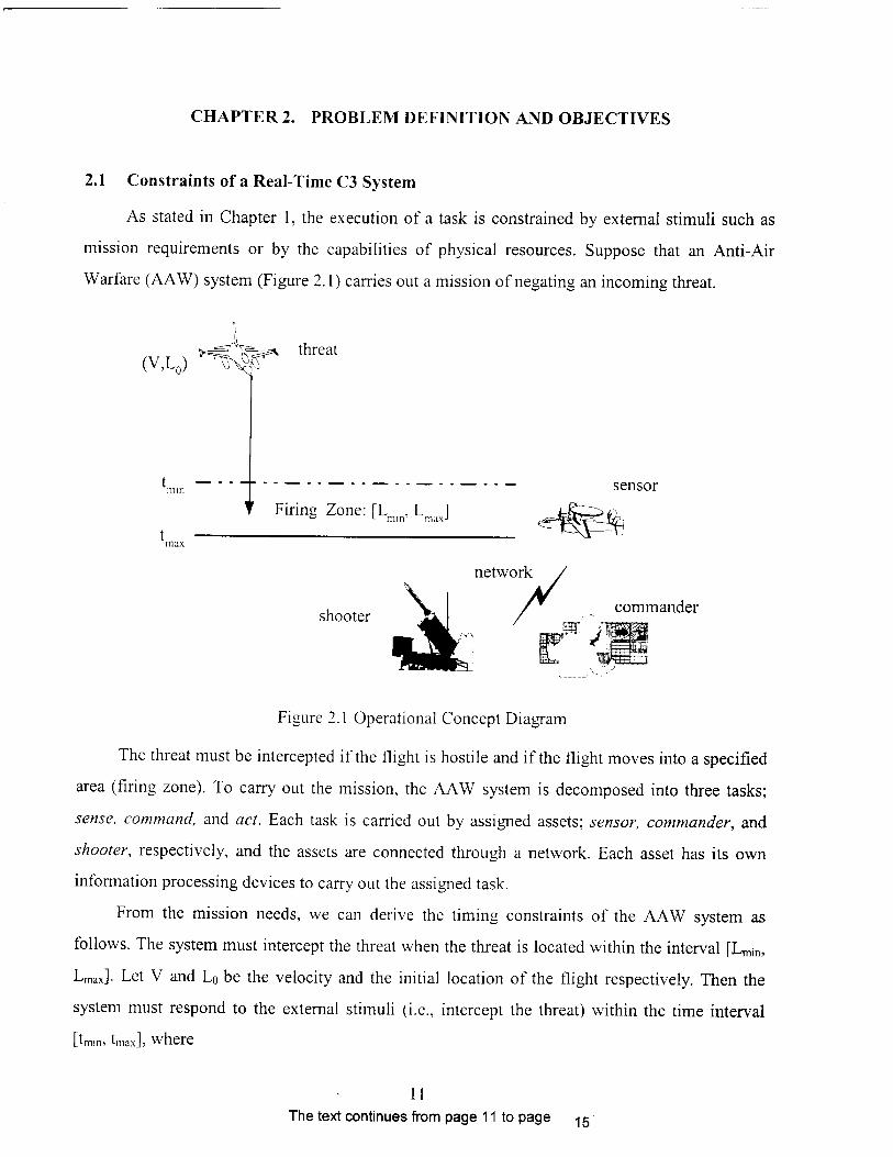
As stated in Chapter 1, the execution of a task is constrained by external stimuli such as

mission requirements or by the capabilities of physical resources. Suppose that an Anti-Air

Warfare (AAW) system (Figure 2.1) carries out a mission of negating an incoming threat.

(V,L0) ^S threat

t Firing Zone: [L . , L 1 ° L mm' maxJ

network

shooter

sensor

commander

Figure 2.1 Operational Concept Diagram

The threat must be intercepted if the flight is hostile and if the flight moves into a specified

area (firing zone). To carry out the mission, the AAW system is decomposed into three tasks;

sense, command, and act. Each task is carried out by assigned assets; sensor, commander, and

shooter, respectively, and the assets are connected through a network. Each asset has its own

information processing devices to carry out the assigned task.

From the mission needs, we can derive the timing constraints of the AAW system as

follows. The system must intercept the threat when the threat is located within the interval [Lmin,

Lmax]- Let V and L0 be the velocity and the initial location of the flight respectively. Then the

system must respond to the external stimuli (i.e., intercept the threat) within the time interval

[tmin, tmax], where

11 The text continues from page 11 to page -jg

'■* = (4* ~h)IV and t^ = (L^ -L0)/V (2.1)

This is the timing constraint of the AAW system. The AAW system must respond to the

threat after tmjn but before tmax. This response must match the desired goal of the mission. In

Andreadakis (1988), the degree to which the actual response matches the desired or ideal

response was defined as the "accuracy" of the response. The accuracy of the response is another

constraint on the AAW system. In the example scenario, the mission needs statement "the threat

must be negated if the flight is hostile" specifies the required accuracy of the response.

2.2 Measuring the Performance of a Real-Time C3 System

A C3 system is not just an information system but also a man-machine system. The

performance of a C3 system cannot be measured by the behavior of the physical components

only. We also have to consider the behavior of the humans. In Miller (1969) and Sheridan and

Ferrel (1974), human decision makers are limited in their capacity to process information and

make decisions (quoted from Andreadakis, 1988). This limitation is called bounded rationality

(Simon, 1976). If we consider this cognitive processing as another type of information

processing , then information theoretic measures can be used. The performance of the

information system can be measured by the data processing delay, the distribution delay of the

messages, and the cognitive processing delay of the decision maker (i.e., task executor). Both

data processing and distribution delays are related with the magnitude of the data, while the

cognitive processing time is related to the semantics of the information or symbols. Levis (1995)

expressed the bounded rationality of human decision maker quantitatively by the rationality

threshold Fo. FQ is the maximum processing rate of the human decision maker, and is expressed

in bits /sec. The processing time t required by a process, whose total activity is G bits/symbol, is

computed by dividing the workload by the processing rate, F, of the human decision maker.

G ' = J (2-2)

and has units of sec/symbol. The minimum processing time, to, corresponds to the maximum

processing rate FQ.

A decision-making organization can be seen as an information processing system that performs a series of tasks to accomplish its mission (Andreadakis, 1988; Levis, 1991).

15

To verify whether the system meets the constraints, we need to be able to measure the

performance of the information system in the perspectives of both time and accuracy. The

accuracy of the response is associated with the semantics of the information (e.g., the content of

reports, the quality of data, credibility of source, etc.) in the information system, while the timing

of the response is associated with complexity of the calculation and the magnitude of the

information (e.g., the number of messages, the size of data, etc.) in the information system. The

objective of this dissertation is to estimate the network connection delay. Hence the size of data

is considered because the transmission delay in a communication network depends on the size of

the messages to be transmitted.

In general, the analysis of a system specification can be done in two phases: the functional

analysis and the timing analysis phases. Functional analysis is performed first to ascertain the

correctness of the logical behavior of the system. Timing constraints are then postulated between

the external stimuli and the response. By specifying the logical behavior as the computation of

the semantics (or symbolic computation) in its functional architecture, the functional architecture

can provide a means to measure the correctness of the logical behavior. In other words, the

accuracy of the response can be measured by the logical correctness of the mappings between the

semantics (or symbols) of the information. In the rule of the example scenario in section 2.1, the

mapping between the input conditions {threat = hostile or neutral} and the output actions {order

-fire or not-fire) deals with the semantics of information. Similarly, the timing of the response

can be measured by the physics of the system in the physical architecture. For example, the

timing of the response of an information system can be measured by the mappings between the

workload of the physical systems and the data processing rate of the computing systems and data

distribution rate of the communication systems.

Once the information system receives physical messages, the messages are pre-processed

to provide task executors with the semantics of information. This pre-processing delay of task i is

defined as x(i). After the task is completed, the information system post-processes the symbolic

information resulting from the completion of the task in the form of a physical message to be sent

over the network. This post-processing delay of task i is defined as y(i). The network delays of

messages between task i and taskj are defined as 8(i,j), where i is the source and j is the sink of

the information.

16

If the task executor is a physical component such as a weapon, the task execution time may

be derived easily from the physical characteristics of weapon systems. The time required to carry

out the task i (constrained by its own physical capability of the asset other than information

processing and distribution capabilities) is defined as an action time r(i). A mechanism to derive

this type of time from the physics of weapon systems was well illustrated in Cothier (1984). If

the task executor is a human decision maker, the action can be derived from the rationality

threshold introduced above (Equation 2.2).

Suppose the mission of the AAW system is carried out as a sequence of task executions as

shown in Figure 2.2. Let the tasks 'sense', 'command', and 'act' be represented by tasks i,j, and

k respectively. The total response time (Tr) can be calculated as,

Tr = hi) + hj) + hk) + <Vo + sv.j) + SU.k) + ö(kfi) (2-3)

where

• t(n) is the elapsed time at node n calculated by

t(n)=x{a)+T(n)+y(B), (2.4)

• S(0J) is the initiating time of task i from the time when the external stimulus takes place,

and

• S(k0) is the impact time of task k on the external environment.

Suppose that a surveillance radar (an instance of the asset sensor) has a scanning cycle of 2

seconds, and reports the result to the fire direction commander (an instance of the asset

commander). The fire direction commander issues a firing order to the missile launcher (an

instance of the asset shooter) immediately after the target is reported. The shooter can either take-

off immediately at time t (when it is armed at the arrival time of the firing order), or at time (t +

5) (assuming a loading of 5 time units). The probability of target detection is assumed to be 1.0

when the target exists in the surveillance area. The intercept time of the missile (i.e., the arrival

time of the missile, after being launched from its initial location, at the intercept point in the

firing zone) is assumed to be between the time interval [1,2]. Then we have:

z(s) = [0, 2], z(c) = [0, 0], <a) = [0, 5], <5(0, s) = [0, 0], and <5(a, 0) = [1,2].

17

*e-

commander shooter assets

x(s) I

pre_processing_s()

y(s) ! i

• post_processing_s() rmessage_s(J

action_c

T(C)

.1 x(c) 1 ^ pre_processing_c()

i i i

post_processing_c() rmessage_c(j

information systems

response()

6(a,0)

pre_processing_aO

pre_processing_a()

Figure 2.2 Operational Sequence Diagram of AAW System

Now, if we can predict the data processing time (x and v) and the network delay of the

information system (S), we can predict the total response time interval Tr (the window of

capability), and verify whether the system responds within the allowed time interval Ta (the

window of opportunity).

Tr can be defined as the time interval:

Tr = ^0, s) + [ r(s) + A(s, c) + z(c) + A(c, a) + z(a) + zl(a, 0)]

where

A(s,c) = [x(s)+y(s) + ö(s,c)],

A(c, a) = [x(c) +Xc) + ^c, a)], and

zl(a,0) = [x(a)+Xa) + ^(a,0)].

18

From the operational concept of Figure 2.1 and Equation 2.1, Ta is defined as the time

interval:

Ta = [tmin, W], where tmin = (Zmin -L0)/V and tmm = (Zmax -I0)/F

Once we can predict the connection delay A(i, j) between functional task i and task] from

the post-processing time v at resource i, the pre-processing time x at resource j, and network

delay <^i, j) between physical resource i and resource j (as constrained by the capabilities of the

physical systems), we can verify whether the system meets the timing constraints, (i.e., whether

the window of capability overlaps with the window of opportunity).

There are two types of decisions in a C3 system; command decision and situation

assessment. A command decision is a mapping from an input condition to an output action. The

rule of "if the threat is hostile then fire, otherwise ..." specifies the command decision. This rule

maps the symbol "hostile" to the symbol "fire". A situation assessment is an informational

judgment about the value of information. It may be associated with the credibility of the

information sources. Making a judgment about whether the threat is hostile or not requires a

decision threshold. The desired level of quality is determined by the decision threshold used to

specify the rule or mapping. The quality of the current information can be measured by the

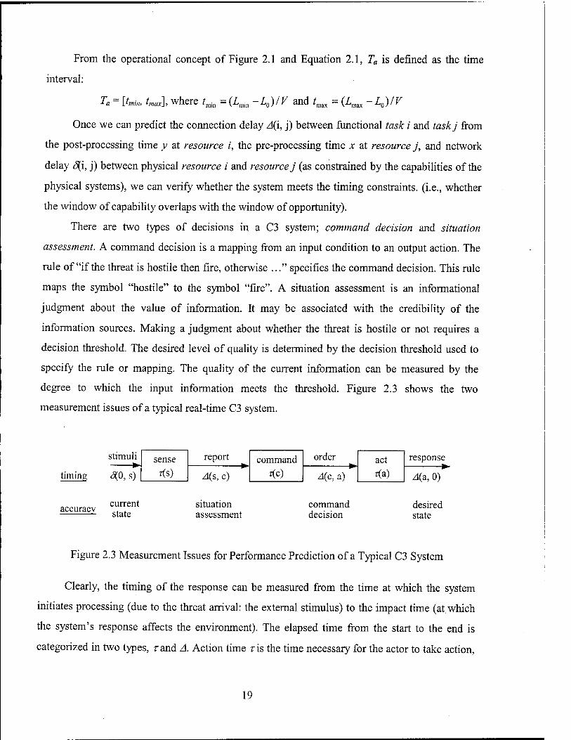
degree to which the input information meets the threshold. Figure 2.3 shows the two

measurement issues of a typical real-time C3 system.

stimuli sense <s)

report command <c)

order act <a)

response

timing 30, s)

current state

A(s, c)

situation assessment

A(c, a)

command decision

A(a, 0)

accuracy desired state

Figure 2.3 Measurement Issues for Performance Prediction of a Typical C3 System

Clearly, the timing of the response can be measured from the time at which the system

initiates processing (due to the threat arrival: the external stimulus) to the impact time (at. which

the system's response affects the environment). The elapsed time from the start to the end is

categorized in two types, rand A. Action time ris the time necessary for the actor to take action,

19

and delay time A is the time necessary for the supporting information systems to process and

distribute the information.

The accuracy of the response can be measured by the degree of the state change toward the

desired state at the response time. When the C3 system is defined as an information system, the

response time of the C3 system can be measured by the timeliness of the information arrival and

the final state of the information system. Defining the level of the desired quality of information,

the degree of state change may be measured by the difference between the desired quality of

information and the current quality of information produced by the information system.

If the information processing is a deterministic process, we can verify the accuracy and

timing of the response separately. One of the robust techniques for verification of the timing

behavior has been well studied in Zaidi's (1999) work. The TL/PN (Temporal Logic and Petri

Net) approach transforms the system's specifications given by temporal statements into a graph

structure. Once the system is verified for correctness, the "Temporal Inference Engine" infers

temporal relations among the system's intervals, identifies the windows of interest to the user,

calculates lengths of intervals and windows, and infers actual time of occurrence of events.

2.3 Research Problem and Objective

Commanders in the battlefield make a decision in the presence of uncertainty as well as

timing constraints. Levis and Athans (1988) defined the uncertainty as the difference between

what one needs to know and what one knows.

U = KN - KA

where KN represent the knowledge needed to carry out a mission, or solve a problem, or make a

decision effectively, and KA represent the knowledge that a decision making entity has at the

point in time and place that a choice needs to be made.

Uncertainty generally reaches an acceptable level after the required action time is past (Van

Trees, 1989) as shown in Figure 2.4. If the level of uncertainty reaches an acceptable level (i.e.,

decision threshold), the decision-maker makes a decision using this information. Meanwhile, the

allowed time (i.e., window of opportunity) to make a decision may close before the uncertainty

reaches an acceptable level.

20

i 1 i allowed •4-» G

<u o c D

j time

\ J acceptible

la \ j. uncertainty

dec

■—' ► tdec K time

Figure 2.4 Uncertainty vs. Time

Consider a decision making process that is state dependent and adaptive to the tempo of

operations. If the tempo of operations becomes higher, the number of messages in a given time

interval increases and the arrival rate of messages to the communication network becomes

higher. Depending on the tempo of operations, the node processing delay and network

transmission delay of the supporting information system will vary.

Maintaining functionally correct end-to-end values may involve a large set of interacting

components. To ensure that the end-to-end constraints are satisfied, each of these components

will, in turn, be subject to its own intermediate timing constraints (Gerber et al., 1994). For

example, multiple sensors can be geographically dispersed to cover the broad range of the

battlefield and configured with various data fusion algorithms for different functional purposes.

Figure 2.5 is an example of a data fusion net for a target identification function and target

tracking function.

If task 4 (i.e., the target identification task) and task 6 (i.e., the target tracking task) in the

figure require all information from the preceding tasks, task 6 cannot be started before task 4 and

task 5 are completed. Depending on the data fusion rule, task 4 may need only partial information

and can be started before all of the tasks in the set {1,2,3} are completed. Depending on the

designed logical behavior of the system, the order of task execution varies. The functional

property of the system generates different orders of message-passing among multiple tasks over a

network and may cause different connection delays between tasks and vice versa.

21

1:IMINT reports Target is enemy

2:SIGINT reports Target is enemy

3 :ELINT reports Target is enemy

5: Tracking radar reports trajectory

4:Target is enemy

6: The target moves to a firing zone

Figure 2.5 A Data Fusion Net

Verifying that the window of capability meets the window of opportunity requires

estimation of the bounded values of the "connection delays" between tasks over a network for the

different tempos of operations, the different orders of task executions, and the different decision

thresholds (depending on the decision threshold of the acceptable level of uncertainty, the

decision making time varies and results in different message generation times).

If the physical communication link between tasks is simply an immediately adjacent

transmission link, the modeling effort may be easy. In Cothier (1984), the network delay was

composed of a set of link delays. If arbitrary values are assigned to each link delay, the minimum

and maximum network delay can be computed from the sum of the link delays. The operating

scheme of each link was represented as a decision tree with associated probabilities. Probabilities

of reliability and survivability were used to represent the availability of each link at the operating

time; the network delay was computed from the reliability and survivability functions in the

decision tree. Suppose that the network is operating using specific protocols and priorities, and

the information has its own data types for different information systems (such as image

processing and message handling), and multiple connections share common network resources

other than single, immediate, adjacent transmission links. The cost of modeling would be very

high and, in some cases, modeling the contention of communication resources maybe practically

impossible.

22

The objective of this thesis is to present an effective method for estimating the connection

delays between tasks so that the performance of a real-time distributed system (both in terms of

timing and accuracy of response) that performs multiple tasks can be predicted.

23

CHAPTER 3. THEORETICAL BACKGROUND

3.1 System Architecting

Systems architecting is the process of creating (conceptualizing, designing, and building)

unprecedented, complex systems (Rechtin, 1991). Levis and Wagenhals (2000) describe a three-

phase system architecting cycle: Analysis-Synthesis-Evaluation. Figure 3.1 shows the system

architecting process.

Mission Operational

Concept

Anaylysis

Functional Architecture

Process Model

D A T A

Data Model

Rule Model

Dynamcis Model

Organization

Physical Architecture

Synthesis

Executable Model

Evaluation

MOPs MOEs

Figure 3.1 A Three-Phase System Architecting

An architecture is defined as the structure of components, their relationships, and the

principles and guidelines governing their design and evolution over time (IEEE STD 610.12).

The architecture development process starts with an Operational Concept. The Operational

Concept specifies what the mission is, the type of tasks it will carry out, and how it is to be

25 Q+JL.l»$*fA*

carried out. The mission and the operational concept induce functional requirements as well as

some physical system and organizational requirements.

At the analysis phase, both static functional and physical architectures are specified. The

functional architecture is a set of activities or functions arranged in a specified (partial) order

that, when activated, achieves a defined goal. The physical architecture is a set of physical

resources (nodes) that constitute the system and their connectivity (links) (Levis and Wagenhals,

2000). At the synthesis phase, both static functional and physical architectures are combined for a

given operational concept and an executable model is developed. Finally, behavior analysis and

performance evaluation can be carried out using scenarios consistent with the operational

concept. A scenario is a sequence of expected events following from a certain input stimulus (or

set of stimuli), and a certain initial state.

The first step in the development of a functional architecture is Functional Decomposition.

This decomposition is a partitioning process and is carried out until each function can be

allocated to a single physical resource (Levis, 1991). Functions necessary for the execution of the

mission as prescribed by the operational concept are identified and further decomposed into sub-

functions that need to be performed. The set of sub-functions has to be mutually exclusive and

possibly exhaustive.

A well-established model for representing functional architectures is the Activity Model

while IDEFO (i.e., Integrated Computer Aided Manufacturing (ICAM) DEFinition language 0;

FTPS 183) is an appropriate language for describing the model. The activity model is derived by

specifying the data exchanged between sub-functions. It shows the flow of information through

the system from inputs from the environment to outputs to the environment. The syntax of the

IDEFO diagram is shown in Figure 3.2.

In IDEFO, a box represents an activity or a function, and arrows or arcs represent flows of

materials, flows of information, interconnections, interfaces, and feedback. There are four types

of arcs: Input arcs, Control or Constraint arcs, Output arcs, and Mechanism arcs. Consequently,

the IDEFO diagram represents up to four relations between functions. In developing the

functional architecture, only inputs, outputs, and controls are modeled; mechanisms are obtained

from the physical architecture.

28

Cl

1 Transform 11 & 12 into 01,02 & 03

as determined by Cl using Ml 11

12

01

02

03

Ml

Figure 3.2 Syntax of IDEFO Diagram

Figure 3.3 is an example of the architectural specifications of a typical C4ISR system in the

abstract and static level. The static functional architecture shows three tasks and their logical

interactions. The static physical architecture shows the assets and their physical interconnections.

surveillance directive engagement rule

Functional Architecture

Physical Architecture

negated threat

network

Figure 3.3 An Example of Architecture Specifications

29

But the performance prediction model requires the synthesis of both functional and

physical models. The process model of IDEFO lacks timing and triggering information which is

required for the performance model. As shown in Figure 3.1, an executable model for

performance prediction requires the synthesis of the data model (specifying the relations between

data), the rule model (specifying the conditions under which functions are performed), and the

dynamics model (specifying the order in which they are performed). It also needs the allocation

of resources (i.e., assets) to functions, in addition to the flow of data.

The properties of the executable model from the functional architecture can be used to

verify the logical behavior (i.e., accuracy of the response). The properties of the executable

model from the physical architecture can be used to verify the timing behavior (i.e., timing of the

response). The assets play the role of interface between the two models.

In a military command and control system, there are three types of measurements for a

system evaluation: (Levis and Wagenhals, 2000)

• Measures of Performance (MOPs): quantities that measure attributes of system

behavior

• Measures of Effectiveness (MOEs): quantities that measure how (well) the system

performs its function

• Measures of Force Effectiveness (MOFEs): quantities that measures how well the

force of which the system is a part performs the mission

MOPs are specified within the boundary of the system and the MOEs and MOFEs are

specified outside the boundary of the system. To measure effectiveness, one must establish

requirements. The requirements must be expressed in a form that is commensurate with the

MOPs. Then MOEs are obtained by comparing the MOP values to the requirements.

MOE = f (MOPs, Requirements)

Alternatively, the MOE may have an implicit standard (e.g., the MOE as an index)

embedded in its definition that reflects the requirements. Suppose that the current variance of

estimated location at time t is St and a launched missile can negate the target if the variance is

less than Sa. Given the requirements Sa, MOPs of the target tracking system can be expressed as

St and MOEs of the target tracking system can be measured by

30

[0 otherwise]

3.2 Petri Net Theory

As stated, a mission is structured as a set of tasks. The set of tasks or functions may be

performed sequentially or concurrently in a distributed computing environment over a network.

Petri nets are a mathematical modeling tool for describing and analyzing discrete event systems

that are characterized as being concurrent, asynchronous, distributed, parallel, non-deterministic,

and/or stochastic (Murata, 1989). Since information processing in distributed discrete event

systems exhibits such properties, Petri nets have been used for their modeling (Tabak and Levis,

1985). The graphical nature of the Petri net helps to easily visualize the complexity of a system,

and the executability allows the system to be simulated to observe its complex behavior and to

measure its performance.

3.2.1 Basic Definitions

Multi-Set

A multi-set m, over a non-empty set S, is a function m E [S-> N]. The non-negative

integer m(s) € N is the number of appearances of the element s in the multi-set m. We usually

represent the multi-set m by a formal sum:

s<=S

By SMs we denote the set of all multi-sets over S. The non-negative integers {m(s) \seS}

are called the coefficients of the multi-set m, and m(s) is called the coefficient of s.

Multi-Set Operations

Some operations of multi-set are defined as:

• Addition:

m\ + m2 = ^ (m{ (s) + m2 (s)Ys. seS

• Comparison:

m\*m2 3s e S : m^s) * m2(s)

31

m\<m2 Vs e S : mx(s) < m2(s).

Subtraction:

m\ - mi = 2^ (w, (s) - m2 (s)Ys , when mi <

Petri net

A Petri net is a bipartite directed graph represented by PN = (P, T, I, O), where

• P = {pi, p2, .., pn} is a finite set of places.

• T = {ti, t2,..., tm} is a finite set of transitions.

• I is a mapping from P x T to N, where N is the set of non-negative integers,

corresponding to the set of directed arcs from places to transitions. I(p,t) = 1 means

that the transition t is connected the place p, in the sense that there exists a directed

arc from p to t.

• O is a mapping from T x P to N, corresponding to the set of directed arcs from

transitions to places. 0(t,p) = 1 means that there exists a directed arc from t to p.

Ordinary Petri net

A Petri net is said to be ordinary if and only if the mappings I and O take their values in the

set {0, 1}.

Pure Petri net

A Petri net is said to be pure if and only if it has no self-loop (i.e., no place can be both an

input and an output of the same transition).

An example of pure ordinary Petri net is shown in Figure 3.4. A place is depicted by a

circle, a transition by a filled bar, and an arc by a directed line segment. The structure of the net

as defined by the quadruple is:

• p= (Pl> P2> P3,P4, P5}.

• T= {ti> h, h, t4, t5}_

• I(Pl,t2)=l; I(P2,t4)=l; I(P3»t5)=l; I(P4.t3)=l; I(P5.t2)=l; all other I = 0.

• 0(tbPl)=l; 0(t2, p2)=l; 0(t2, p3)=l; 0(t3, Pl)=l; 0(t4, p5)=l; 0(t5, p4)=l; all

other O = 0.

32

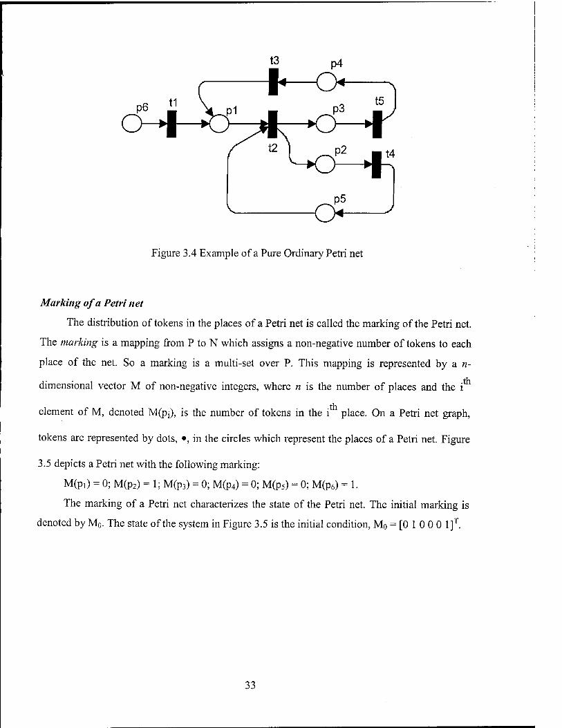
Figure 3.4 Example of a Pure Ordinary Petri net

Marking of a Petri net

The distribution of tokens in the places of a Petri net is called the marking of the Petri net.

The marking is a mapping from P to N which assigns a non-negative number of tokens to each

place of the net. So a marking is a multi-set over P. This mapping is represented by a n-

dimensional vector M of non-negative integers, where n is the number of places and the i

element of M, denoted M(pj), is the number of tokens in the i place. On a Petri net graph,

tokens are represented by dots, •, in the circles which represent the places of a Petri net. Figure

3.5 depicts a Petri net with the following marking:

M(pi) = 0; M(p2) = 1; M(p3) = 0; M(p4) = 0; M(p5) = 0; M(p6) - 1.

The marking of a Petri net characterizes the state of the Petri net. The initial marking is

denoted by M0. The state of the system in Figure 3.5 is the initial condition, M0 = [0 1 0 0 0 1]T.

33

Figure 3.5 Example of Markings of Petri net

Enabling of Transitions

A Petri net executes by firing transitions. In order to fire, a transition must be enabled. A

transition is said to be enabled for a marking M, if and only if, for each place of the net:

M(p,) > I( Pi, tj) for all Pi e I(p, ,tj)

Firing of Transitions

Any change in the marking and, therefore, any change in the state, is controlled by

transitions. When the transition is enabled, it can fire. When it fires, tokens are removed from

each of its input places and tokens are put in each of its output places. Firing of the transition tj

results in a new marking M' where:

M'(pi) = M(Pi) - I(Pi, tj) + 0(tj, pi) for all Pi e I(Pi ,tj) and for all p, e 0(tj, Pi)

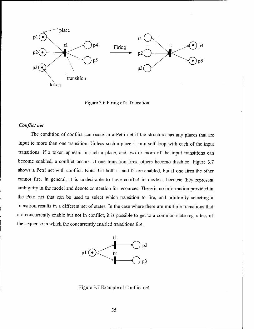
Figure 3.6 shows an example of the firing of a transition. Transition tl is enabled because

there is at least one token in each of its input places, pi, p2, and p3. When tl fires, one token is

removed from each of the input places of tl and tokens are added to each of the output places, p4

and p5. The firing of transitions causes the marking of the net to change from [1 1 1 0 0]T to [0 0

Oil] and therefore introduces a change in the state of the system.

34

place

transition

Firing

token

Figure 3.6 Firing of a Transition

Conflict net

The condition of conflict can occur in a Petri net if the structure has any places that are

input to more than one transition. Unless such a place is in a self loop with each of the input

transitions, if a token appears in such a place, and two or more of the input transitions can

become enabled, a conflict occurs. If one transition fires, others become disabled. Figure 3.7

shows a Petri net with conflict. Note that both tl and t2 are enabled, but if one fires the other

cannot fire. In general, it is undesirable to have conflict in models, because they represent

ambiguity in the model and denote contention for resources. There is no information provided in

the Petri net that can be used to select which transition to fire, and arbitrarily selecting a

transition results in a different set of states. In the case where there are multiple transitions that

are concurrently enable but not in conflict, it is possible to get to a common state regardless of

the sequence in which the concurrently enabled transitions fire.

Figure 3.7 Example of Conflict net

35

3.2.2 Algebraic Representation

Incidence Matrix

The structure of Petri nets can also be represent algebraically by an integer matrix C, called

an incidence matrix. C is an n x m matrix whose m columns correspond to the transitions and

whose n rows correspond to the places of the net. The elements Cjj of the incidence matrix C are

defined as follows:

Cij = 0(tj,pi)-I(pi,tj) forl i n,\ j m.

The incidence matrix of the Petri net in Figure 3.4 is given below. Note that the rows and

columns of the matrix have been annotated with the corresponding places and transitions for

clarity.

Pi P2

C(PN) - p3 p4 p5 p6

tl t2 t3 t4 t5 1-110 0 0 10-10 0 10 0-1 0 0 10 1 0-101 0 -10 0 0 0

The value attributed to each cell describes the relation between the corresponding places

and transition. In the case of ordinary Petri nets, Qj takes values in (-1 0 1} only

• -1 indicates that the place is an input place to the transition,

• 1 indicates that the place is an output place of the transition, and

• 0 indicates that there is no arc connecting the place to the transition.

It should be noted that self-loops cannot be accounted in this representation. If t; and pj

form a self-loop, then we have I(p, tj) = 1 and 0(tj, p) = 1, and therefore Qj = Q. Consequently,

the incidence matrix represents uniquely only pure Petri nets.

While it is possible to illustrate the dynamics of a Petri net by graphically showing the

change in the marking as transitions fire, it is also possible to mathematically calculate the

change of the marking of a Petri net using the incidence matrix and linear algebra. To see this,

two notions are needed, the firing sequence and the firing vector.

Firing Sequence

A firing sequence defines a sequence of ordered firings. It is represented by

36

CTs = tj ' tj • tk ...

This means that tj fires first, then tj, then tk. The firing sequence is simply a list of transitions in

the order in which they fire.

Firing Vector

A firing vector, Ns, can be associated with a firing sequence as. Ns is a column vector

whose dimension is equal to the number of transitions, m. The i-th element of Ns denotes the

number of occurrences of transition tj in the firing sequence as. Note that a firing sequence can

always be used to generate a firing vector, but the converse is not true, because the firing vector

does not have any indication of the sequence in which the firings take place.

Given a marking M, the incidence matrix C, and a firing vector Ns that corresponds to a

firing sequence os, the resultant marking M' of the firing sequence can be calculated algebraically

by:

M' = M + ONs

Reachable Marking

Given an initial marking Mo of the net, a reachable marking is any possible marking of the

net which can be obtained from the initial marking. In other words, given a net and initial

marking M0 for this net, M is a reachable marking if and only if there exists a firing sequence a

such that:

Mo »M

Or there exists an Ns corresponding to the firing sequence cr such that:

M = M0 + ONs

For example, suppose that the initial marking of the net of Figure 3.5 is,

M0 = [0 1000 1]T.

A valid firing sequence is to fire each of the transitions in the sequence

CTS = ti * t4 • t2 • t5 • t3.

T The corresponding firing vector is: Ns = [1 1 1 1 1]

The marking M reached by this firing sequence is obtained by:

37

M = +

1 -1 1 0 0 1 0 -1 0 1 0 0 0 0 -1 0 0 -1 0 1 -1 0 0 0

0 0

-1 1 0 0

0 1 1 1 0 1 0 0

+ 0 0 =

0 0

0 0 0 1 -1 0

This equation indicates that after the firing sequence Ns, the resulting marking has one

token each in places pj and P2 while the other places have no tokens.

However, this approach should be used with caution in order to avoid its two main pitfalls:

• As noted previously, self-loops cannot be accounted in the matrix representation of

the net

• The firing vector must correspond to a feasible firing sequence.

Reachability Set

Given an initial marking M0 of a Petri net, the reachability set - denoted 5R(M0) - is the set

of all possible reachable markings. In other words, a marking M belongs to 9?(M0) if there exists

a firing sequence a leading from M0 to M.

3.2.3 Occurrence Graph

The occurrence graph is another means of depicting reachability. In this graph, the nodes

represent the state (marking) of the net and the directed arcs indicate the firing of an enabled

transition in a state causing the state to change. These directed arcs are called occurrences. Each

occurrence in the occurrence graph represents the firing of a single transition. Thus an occurrence

graph is a state transition diagram.

An example of an occurrence graph is shown in Figure 3.8. This graph was generated from

the Petri net of Figure 3.5 with the initial marking M0 = [0 1 0 0 0 1]T.

The occurrence graph shows all the reachable markings^ro/w the given initial state. Thus, it

contains the reachability set of the net for the given initial marking. Different occurrence graphs

will be generated for different initial markings. It also shows all of the legitimate firing

sequences. Each firing sequence is a path through the graph. For example, the firing sequence as

38

= ti • t4 • t2 • t5 • t3 is shown as a path on the right hand side of the graph: Mo - M2 - M3 - M4

M6 - M2.

M, ([010011]

M, [1 10 000]^—.

t3

W[o 1 1000] ^ t3

Figure 3.8 Example of Occurrence Graph

3.2.4 Timed Petri Nets

In ordinary Petri nets, time is not included: transitions fire either in sequence or

concurrently, but nothing says when these firings are taking place. An extension of ordinary Petri

nets is Timed Petri nets where time is introduced to model delays associated with processes or

buffers. Two approaches are possible: the place model and the transition model. In timed Petri

nets, the time can be introduced either at a "transition" or at "places". It can be proved that

assigning processing times to places is equivalent to assigning processing times to transitions

(Sifakis, 1980).

39

Place Model of Time

In the place model, a delay is associated with each place and corresponds to the delay

associated with buffers. Tokens are in one of two states: available or unavailable. If Ma denotes

the marking of available tokens in a place and Mu the marking of unavailable tokens, the total

marking M of a place is: M = Ma + Mu. A transition is enabled only by available tokens. When a

transition is enabled, it fires instantly: the enabling available tokens are removed from the input

places and unavailable tokens are generated in the output places. These tokens remain

unavailable for a time equal to the delay associated with the place in which they reside.

Transition Model of Time

In the transition model, a delay is associated with each transition and corresponds to the

delays of processes. Tokens are in one of two states: reserved or unreserved. If Mur denotes the,

marking of unreserved tokens in a place and Mr the marking of reserved tokens in the same

place, the total marking M is: M = Mr + Mur. A transition is enabled only by unreserved tokens

present in the input places. When a transition is enabled, firing is initiated and the enabling

tokens become reserved during a time equal to the delay associated with the transition. When the

firing terminates, the reserved tokens are removed from the input places and unreserved tokens

are generated in the output places.

Timed Occurrence Graph

An ordinary Petri net has no notion of time. Neither does it contain any information about

the order in which concurrently enabled transitions will fire. Because this information is not

contained in the Petri net, the occurrence graph shows all of the possible states that the system

could encounter. In a Timed Petri net, the state of a system can be represented by a «-dimensional

state vector in which a state is a pair (M, r) where M is a marking and r is a time value. The

initial state is the pair S0 = (M0, r0) and the sets of all states are denoted by S. In the timed

occurrence graph of a Timed Petri net, each node contains a time value in a timed marking.

40

3.3 Execution of Distributed Systems

3.3.1 Causality vs. Time

If the execution of an event A causes or effects the execution of event B, then the execution

of A and B must be scheduled in real time so that A is completed before B starts. Violation of this

constraint is referred to as a causality error (Unger et al., 1993). A distributed simulation system

must explicitly coordinate the advance of time in order to maintain temporal consistency between

the components. Human beings use the concept of causality to plan, schedule, and execute an

enterprise, or to determine a plan's feasibility. The notion of time is basic to capturing the

causality between events.

In daily life, we use global physical time to deduce causality. However, distributed

computation systems have no built-in global physical time. In the execution of distributed

computation systems, the notion of time can be viewed in terms of virtual time and a logical

time. The virtual time is a counterpart of a physical clock such as a wall-clock. The logical time

is derived to capture the causal precedence relation between events. The logical time is defined at

the level of temporal semantics in terms of event ordering (Carroll and Borshchev, 1996).

A logical clock is a data structure coupled with a function (i.e., protocol) in which the

function is used to update the clock (i.e., the data structure) when an event is executed

(Kalantery, 1997). In a logical clock, every event is assigned a time stamp, by which a process

can infer the causality relations between events. The time stamp can be defined as Scalar, Vector,

or Matrix in its data structure.

In Raynal and Singhal (1996), the logical time system consists of a time domain T, and a

logical clock C. Elements of T form a partially ordered set over a relation <. This relation is

usually called "happened before" or causal precedence. The logical clock C is a function that

maps an event e in a distributed system to an element in the time domain T, denoted as C(e) and

called the time stamp of e. The clock C is defined as:

C:Ha T

where H is a set of events in a distributed system, to satisfy the following property:

ei -» ej => C(e,) < C(e;) for all i andy, and / *j .

41

The binary relation -» defines a total order on events and expresses causal dependencies among

the evens. The time stamps assigned to events obey the fundamental monotonicity property. That

is, an event a causally affects an event b, then the time stamp of a is smaller than the time stamp

of b. This monotonicity is called the clock consistency condition. When T and C satisfy the

following condition,

ei -> e} c> C(ei) < C{e}) for all / and j, and / *j .

the clock is said to be strongly consistent.

The causal relationships in a distributed system yield only a partial order. Lamport (1978)

proposed a scalar time representation for totally ordering events in a distributed system. In his

scalar time representation, the time domain is a set of non-negative integers. The protocol to

update the clock consists of two rules. Rules Rl and R2 update the clock as follows, (quoted

from Raynal and Singhal, 1996)

• Rl. Before executing an event, pi executes the following:

q-q+d (d>0)

In general, every time Rl is executed, d can have a different value, which can be application-

dependent. However, d is typically kept 1, since this allows a process to identify the time of each

event uniquely at a process while minimizing J's rate of increase.

• R2. Each message piggybacks the clock value of its sending time. When a process

Pi receives a message with the time stamp Cmsg, it executes the following actions:

Before executing an event, pt executes the following:

1. C,.:= max (C,.,CmJ 2. Execute Rl 3. Deliver the message.

The main problem in totally ordering the events is that two or more events at different

processes can have the identical time stamp. In Figure 3.9, for example, event c of process pi and

event j of process p2 have the same time stamp; the same occurs for event / of process p2 and

event x of process P3.

Genuinely, concurrent events have no influence on one another (Fidge, 1991). Since both

events c andy are independent (i.e., not causally related), the system can order them using any

criterion without violating the causality relation. We can order them using the process identifier.

42

12 3 8 9

Figure 3.9 Evolution of a Scalar Time in Distributed Execution (d=l)

Let the time stamp of an event be denoted by a tuple (t, i), where t is its time of occurrence

and i is the process at which it occurred. The total order relation 7i on two events x and v with

time stamps (h, i) and (k, j), respectively, is

x n y <=> (h < k or (h = k and / < j)).

Typically, process identifiers are linearly ordered. So, when two events have the same time

stamp, the event at the lower ordered process is ordered lower.

After Lamport (1978)'s scalar time system, many efforts have been made to capture the

causality in distributed systems using Vector time (Fidge,1991; Mattern, 1988; Schmuck, 1988)

and Matrix time (Fischer and Michael, 1982). The comparison and efficient implementation of

their logical time systems are found in the literature (Carroll and Borshchev, 1996; Garg and

Tomlinson, 1994; Raynal and Singhal, 1996).

In distributed algorithm design, the properties of a system of logical clocks and the

causality relation helps in the analysis of a system's functional behavior such as liveness,

fairness, deadlock, concurrency, and consistency check. A total order is generally used to ensure

liveness properties in distributed algorithms (requests are time stamped and served according to

the total order on these time stamps) (Ramport, 1978; quoted from Raynal and Singhal, 1996).

Similar kinds of analysis can be done by temporal logic and Petri nets. In Levis (1998) and Zaidi

(1999), for example, a system is initially specified by temporal logic (first order logic) and the

properties of the system are verified using a Petri net whose structure is equivalently constructed

from temporal logic specifications.

43

For the performance evaluation of a distributed system (especially the timing behavior of

the system), we have to know the processing time of each event at each process. Once we can

measure the processing time based on the capabilities of the processors used to carry out the

processes, we can verify whether the system meets the timing constraints, (i.e., whether the

windows of capability overlaps with the windows of opportunity). One of the robust techniques

for verification of the timing behavior is well studied by Ma (1999) on the extension of Zaidi

(1999)'swork.

3.3.2 A Model of Distributed Execution

In Raynal and Singhal (1996), a distributed program is composed of a set of n

asynchronous processes x¥l, x¥2> ..., xi>n that communicate by message-passing over a

communication network. The execution of x¥i produces a sequence of events:

e° ex ex ex+l

denoted by Ht where

#,=(*„->,).

The set of events produced by *P;. is ht. The binary relation -»,. expresses causal

dependencies among the evens ht of process x¥i. The events are classified into three types:

internal event, send-message event, and receive-message event. An internal event affects only

the process at which it occurs, and the events at a process are ordered by their order of

occurrence. So the binary relation ->(. defines a total order on ht. Events Send-message and

receive-message signify the flow of information between processes and establish causal

dependency between the sender process and the receiver process. Consequently, the execution of

a distributed application results in a set of distributed events produced by the process. A relation

~^msg is defined to represent the causal dependencies between the pairs of corresponding send-

message and receive-message events. For every message m exchanged between two processes,

we have

send-message(m) —> receive-message(m).

Then the distributed execution of a set of processes is a partial order:

H = (H, -»), where

44

-> = u/ ->/ u -^» and -^ ^ ^.

For example, the distributed system of Figure 3.9 can be modeled:

Hx - (A,, —»,) , where A, = {a, A, c, rf, e) and ->, = {(a, b), (b, c), (c, d), (d, e)},

H2 = (A2,-»2), where A2 = {i,j, k, I, m, n) and ->2 = {(i,j), (/, k), (k, I), (I, m), (m, n)},

Hi = Vh»~>3)» where A3= {^ v< y>z) and ""^3= ((w> x)> (■*> J')» (y»z)}» and

-^™g = {(*»». (*> *), fo <0, (e, w)}.

Then the distributed execution of the system is a partial order:

H = (H, -»), where

H = A, u A2 u A3

If the distributed system processes the events in a total order TT :

7t = {(a,i), (i,w), (w,b), (b,c), (cj), (f,k), (k,l), (l,x), (x,y), (y,z), (z,d), (d,e), (e,m), (m,n)}

it does not violate the causality relation.

3.3.3 Simulation of Distributed Discrete-Event Systems

For a non-distributed discrete event simulation, the notion of simulated time is explicitly

available and the sequential unipocessor simulation (time- or event-driven simulation) is a

straightforward method because the entire system is centralized (i.e., centralized event queueing)

and only one object can be simulated at any given time (i.e., single stepping clocks). This

sequential, unipocessor, discrete event simulation often relies on shared global memory, and its

simulation time is implemented as a global variable (McAffer, 1990). The simulation clock

records the occurrence time (time stamp) of the last input event and is used to calculate a time

stamp for the occurrence of the next output event (Kalantery, 1997).

In the execution of Timed Petri nets, for example, the occurrence of an event relates to the

firing of a transition. The simulation engine maintains an event list (scheduled transition firings).

It repeatedly executes the first event in the list, simulating the behavior caused by the event

(change the virtual time to the event time stamp, change the markings, enable new transitions

and/or disable transitions that were already enabled), inserting (removing) corresponding new

45

events to be scheduled (old events to be descheduled) into (from) the event list, and finally

removing the executed event from the list (Chiola and Ferscha, 1993).

In distributed event-driven simulation, the processes do not share global memory and

communicate solely by passing messages. Unlike conventional sequential programs, the

computations performed by distributed computing systems do not yield a linear sequence of

events. The interrelationships between the events performed in a distributed system is inherently

a partial ordering (Fidge, 1991). So a distributed system must explicitly coordinate the advance

of time in order to maintain temporal consistency between the computations. The system must

define how time is advanced when, according to models, it should be advanced. In real-time

simulation of distributed discrete-event systems, the semantics of the simulation program rely on

the simulation time. The simulation time progresses in a way that avoids violating the causality

relations of the program.

Simulation is a cost-effective approach to performance evaluation of a complex distributed

system. But the simulation of a distributed system must not violate the causality relation among

events. This can be done by using a total ordering of events for the simulation. Clearly, scalar

clocks satisfy monotonicity, and hence the consistency property. We can use the scalar clocks to

totally order events since a total order is consistent with the causality relation as shown in the

previous section.

The general techniques for distributed event-driven simulation guarantee the serializability

of the behavior of a distributed simulation and therefore yield results equivalent to some

sequential simulation (Ricciulli et al., 1996). Simulation techniques of this type are usually

classified as either pessimistic or optimistic. Both of these techniques use the same notion of

local and global virtual time. The local virtual time (LVT) of an object is defined as the time up

to which that object has executed the simulation. The global virtual time (GVT) is the point in

simulation time up to which all components have successfully executed. The GVT at a particular

point in the simulation is equal to the minimum of all the LVTs in the system. If some

component has LVT that is equal to the GVT, then it is said that the component defines the GVT

(McAffer, 1990).

46

Pessimistic Simulation

Chandy and Misra (1981) introduced the pessimistic simulation technique, called

conservative approach, because it assumes that components will communicate out of sequence,

even though some events might have been independent of each other. It guarantees that a

processor does not advance its simulation clock until it is certain that it will not bypass some

simulation time at which another processor affects it. It uses synchronous message passing to

coordinate the concurrent components.

The conservative approach is inefficient because all events simulating global state change

must go through a central controller, therefore creating a serialization blocking. In other words,

messages cannot be received until the receiver's LVT equals to GVT. The message's sender

remains blocked until the receiver defines the GVT. In order to avoid deadlock and to achieve

simulation efficiency, the conservative approach requires "lookahead" which is the ability of a

processor to predict its future behavior, as regards when next (in simulation time) it may affect

another processor's submodel (Nicol and Roy, 1991).

Optimistic Simulation

Jefferson (1985) introduced an optimistic simulation technique, called Time Warp, which

allows parts of a simulation to get ahead of themselves. In contrast to the pessimistic technique,

objects using Time Warp simulate and communicate freely with other components until they

receive a message. If the new message is from the receiver's future (i.e., if the message time

stamp is greater than the receiver's LVT), then the receiver increases its LVT to the message's

time stamp value and processes the message. If the message is from the component's past, then

the receiver must undo, "rollback," any processing it did or messages it sent between its current

LVT and the new message's time stamp value. The rollback procedure relies on the

reconstructibility of past states which can be guaranteed by a systematic state saving policy and

corresponding state saving reconstruction procedures, causing respective overheads (Ferscha and

Richter, 1997).

State saving mechanisms are an essential part of the Time Warp approach for the efficiency

of simulation. Various methods and their comparisons are described in Ronngren et al. (1996)

and Radhakrishnan et al. (1996). Since all message passing is asynchronous, Time Warp is

entirely free of simulation induced deadlock. Time Warp is efficient for loosely coupled, highly

47

asynchronous systems, but is inefficient when models have mixed time scales or diverse

interaction behaviors (McAffer, 1990).

48

CHAPTER 4. A METHODOLOGY TO DEVELOP SYNTHETIC EXECUTABLE MODELS

4.1 The Premises in the Dissertation

An executable model for performance prediction can be developed in various ways. A

straight-forward approach is to develop a single integrated executable model in which network

connection delays and the contention for resources are directly modeled at the functional

architecture level using additional transitions and places as shown in Figure 4.2, as an extension

of the executable functional model of Figure 4.1.

Figure 4.1 An Executable Functional Model as an Ordinary Petri net

In the synthetic execution approach, both functional and physical architectures are modeled

as separate executable models. The central idea of this dissertation is to synthesize layered

architectures using the concept of two state machines communicating with each other. From the

perspective of distributed simulation systems, the performance prediction model of real-time

distributed simulation consists of two processors: one for the C2 model and the other for the

communication model. The proposed approach is not the typical run-time distributed simulation

model because there is no message exchange between the two communicating state machines at

run-time.

49

Figure 4.2 An Integrated Executable Model

The motivation behind distributed simulation is to gain a speedup over traditional

sequential simulation, while guaranteeing equivalent results to those of some sequential

simulation. The two communicating state machines in the problem domain are tightly coupled.

The number of logical communication channels between the two models can be as many as the

number of arcs in the Petri net model. So none of those distributed simulation technique might be

efficient. However, if the messages generated by one model can be totally ordered in the other

model's time domain to guarantee the serializability of events (i.e., total ordering of events), we

can simulate the other model separately "off-line", rather than using distributed simulation at

"run-time". In fact, Jefferson's (1985) optimistic simulation is the converse approach in that that

it specifies a total order on the events, and then provides a mechanism that causes the events of a

computation to be executed in a partial order that conforms to the specified total order.

(Bayerdorffer, 1995)

50

In the problem domain of this dissertation, the network delays are unknown. How can we

capture the precedence relation with the unknown delays? In Petri nets, however, the precedence

relations can be captured by the occurrence graph. Using the information contained in the

occurrence graph, we can capture the traffic pattern and order the messages linearly on the

communications network simulation time domain.

4.1.1 Capturing Precedence Relations from the Occurrence Graph

As defined in the previous chapter, given the current marking M of a Petri net, firing of the

transition t results in a new marking M' where:

M'(pi) = M(pO - I(Pi, t) + 0(t, Pi), for i = 1,..., n.

Suppose that the Petri net is an ordinary net. If we perform a subtraction operation of

markings; M'(pi) - M(pO, the computation results in {+1, 0, -1} as shown in Table 4.1.

Table 4.1 Illustration of Subtraction Operation between Two Markings

0(t, Pi) - I(pi,t) = M'CPO-MCPO

0 0 0

0 1 -l

1 0 +i

1 1 0

The "+" and "-" signs tell whether the token is a newly placed one or a removed one

respectively. Note that this interpretation can be made only on pure Petri nets. If the Petri net is

not pure (i.e., the structure has a self-loop), the "0" in the fourth row occurs. Clearly, one token is

removed and one token is newly generated. But it is not distinguished from the "0" in the first

row that represents no change after the firing of a transition. For example, place p6 in Figure 4.1

has a self-loop and computes the result "0" at the place p6 in Table 4.2.

51

Table 4.2 Subtraction of Marking Vectors from an Occurrence Graph

M0 Mi M2 M3 Mi -Mo M2- Mi M3-M2

M(pi) 1 0 0 0 -1 0 0

M(p2) 1 0 1 1 -1 +1 0

M(p3) 0 1 0 0 +1 -1 0

M(p4) 0 1 1 0 +1 0 -1

M(p5)

M(p6)

M(p7)

1

1

0

I 0 1

1

0

0

0

0

-1 +1

0

-1

1 1 0

0 1 +1

M(p8) 0 0 0 1 0 0 +1

Note that this subtraction of two markings is different from the subtraction of multi-set.

Recall that the subtraction of multi-set is defined as:

m\ - mi = ^ (mx (s) - m2 (s)Ys , when mi < m\ and S is a non-empty set. seS

The operation has the pre-condition mi < ni\. When m\ < m2, the subtraction operation of

multi-set cannot be conducted. By defining the intersection n of two multi-sets as:

m\ n mi = ^ {(minf/W; (s), m2 (s)]Ys | s e mx Asem2} (4.1)

.165

the subtraction operation of two marking vectors Mi and M2 can be defined as:

M, - M2 = 2 {M, (p) - [M, {p) n M2 (p)]} (4.2) peP

where Mj(p) is the marking of place p at the marking vector Mj and P is a set of places.

Remember that a marking is a multi-set over P. Using Equations 4.1 and 4.2, given two

subsequent marking vectors M and M' of pure Petri nets (not necessarily ordinary Petri nets), we

can distinguish new tokens and removed tokens by subtraction of the two marking vectors by:

new token(s) = M' - M and removed token(s) = M- M' (4.3)

If the two subsequent markings M and M' are the ones before and after firing one transition

respectively (i.e., not concurrent firing of multiple transitions) of a pure Petri net, the removed

tokens become the triggering tokens of the new tokens that have the precedence relations

52

between those two sets of tokens. Suppose that Figure 4.1 is an executable functional model

corresponding to the architecture specifications of Figure 3.3. The occurrence graph with an

initial marking Mo = [1 10 0 1 1 0 0]T is shown in Figure 4.3. Table 4.2 is the result of the

subtraction operation of the marking vectors.

M0 = [l 1 0 0 1 1 0 Of JJtl

M, = [0 0 1 1 1 1 0 Of Jit2

M2 = [0 1 0 1 0 1 1 Of Ut3

M3 = [0 1 0 0 1 1 0 if

Figure 4.3 Occurrence Graph of an Executable Functional Model

4.1.2 Total Ordering of Events

The occurrence graph shown in Figure 4.3 was generated by a firing sequence of transitions

a = tl • t2 • t3 in the Petri net shown in Figure 4.2. The executable functional model represents a

mission consisting of a set of tasks {tl, t2, t3}. The sequence of tasks, how the mission is carried

out, is represented by the firing sequence of transitions. The set of events of the executable

functional model maps to the set of transitions {tl, t2, t3}, and the causality between events maps

to the firing sequence: tl —> \2 and t2^ t3. Thus the process of the executable functional model

(PC2) has a total order:

Ha = (äC2,->C2) , where hc2 = {tl, t2, t3} and ->c2 = {(tl, t2), (t2, t3)}.

Let m^Pj) be the marking of place pi at the marking vector Mj. The firing of transitions tl,

t2, and t3 generates a set of new tokens {mi(p3), mi(p4)}, {m2(p2), m2(p7)}, and {m3(p5), m3(p8)},

respectively (identified by the "+" signs in Table 4.2). This set of new tokens plus the initial

tokens {m0(pi), m0(p2), m0(p5), m0(p6)} are the set of messages to be transmitted over the

communication network. The transitions tl, t2, and t3 are conditioned on a set of input tokens

{m0(pi), m0(p2)}, {mi(p3), mi(p5)}, and {m2(p4), m2(p7)}, respectively (identified by the "-" signs

in Table 4.2). So the process of the communication network model has the following causality

between sets of messages:

53

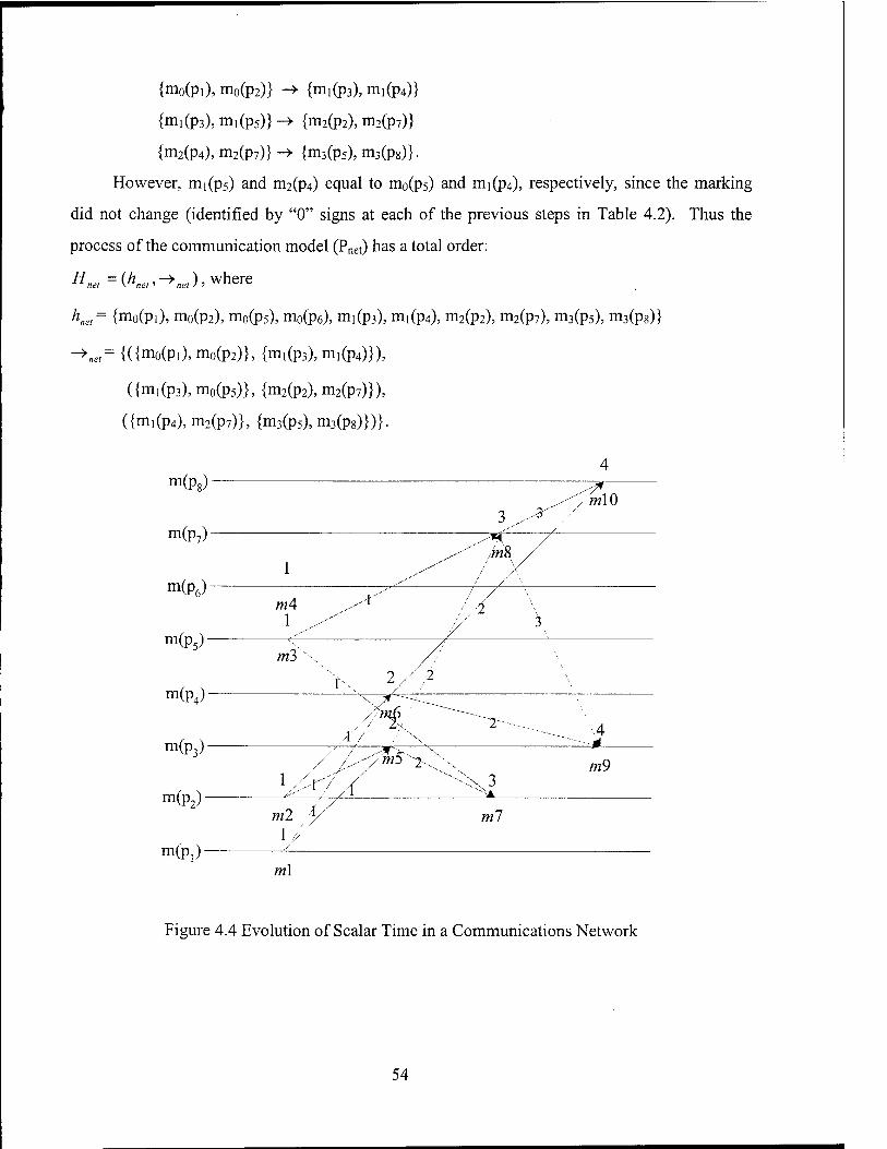
{mo(pi), m0(p2)} -» {mi(p3), mi(p4)}

{mi(p3), mi(p5)} -> {m2(p2), m2(p7)}

{m2(p4), m2(p7)} -» {m3(p5), m3(p8)}.

However, mi(p5) and m2(p4) equal to mo(ps) and nii(p4), respectively, since the marking

did not change (identified by "0" signs at each of the previous steps in Table 4.2). Thus the

process of the communication model (Pnet) has a total order:

Hne, =(hnet,^net), where

h„e,= (mo(Pi), m0(p2), m0(p5), m0(p6), mi(p3), mi(p4), m2(p2), m2(p7), m3(p5), m3(p8)}

-\« = {({mo(Pi),ni0(p2)}, {mi(p3), m,(p4)}),

({mi(p3), m0(p5)}, {m2(p2), m2(p7)}),

({m,(p4), m2(p7)}, {m3(p5), m3(p8)})}.

m(P8) ^-~ : MO

m(p7)

m(P6)"

m(p5) -

m(P4)-

m(p3)-

m(P2)-

m(Pi)-

3 ,/"3"

1

m4 „ r

1 .,/'"

w3 \

x W /f^C^ 2 A

' -'S V *~ / j^ym5 -2^\ m9

l /., / / " :x 3 ^■--•1 'A ^

ml .5/ ml 1,;

ml

Figure 4.4 Evolution of Scalar Time in a Communications Network

54

If we simulate the communication network model using the set of events hnet (i.e., traffic),

while not violating the precedence relation —»ne(, we can measure the network delay as the state

of the system evolves as designed in carrying out the mission. Figure 4.4 shows the evolution of

logical time, using d = 1, at the communications network model.

Note that Figure 4.4 is not a model of distributed computation. It just illustrates the order

of messages. In the figure, a message identification number (mx) is assigned to each message;

first, a sequential integer number is assigned to each initial token at the initial marking vector Mo,

then the number is increased whenever a new token is identified at the next marking vector in the

sequel. The arrow lines represent the precedence relation which defines a total order. Remember

that the binary relation -»,. defines a total order among the events (A;) of a process (Pj) at which

the events occur.

The example of how the logical time stamps are associated with the precedence relations

for simulation will be demonstrated in the next section.

4.1.3 Simulation of Discrete-Event Systems

In a non-distributed system, a logical time system can be derived such that the sequential

position of a message arising from anywhere in the running program is clearly identified by its

time stamp and the time stamps provide a facility to determine the precedence relations between

already received messages (Kalantery, 1997). During the running time of the network model,

messages ml, m2, m3, and m4 in Figure 4.4 can be ordered on a single time line by comparing

their simulation time stamps.

Let F(w()be the virtual time stamp of message w,-. Then we can make an event list (i.e.,

scheduling traffic) by comparing their virtual time stamps. Suppose V(mj) = 4, V(m2) = 3, V(m3)

= 2, and V(m,4) — 1; then the scheduler makes an event list [m4, m$, m2, mf\. If any of these events

is executed,

1) the scheduler deletes the event from the event list,

2) determines the next event, and

3) updates the event list (i.e., reorder the events comparing the time stamp of the new

event and those of events on the event list), and finally

4) the virtual time advances to the time stamp of the first event in the event list.

55

For example, if the event m4 is executed at time 1, the event m4 is deleted on the event list.

It is not supposed to trigger any events. So the virtual time advances to the time stamp 2 of event

ms which becomes the first event on the event list after deletion of the event m4. Step 2 and 3 are

skipped. Because the virtual time has been advanced to the virtual time stamp of event mi, the

simulation engine executes the event ms at time 2.

After the event ms is executed, it is supposed to trigger events mj and m$. But events mz

and ms cannot be executed since the preceding events mj and m2 have not been executed (the

logical time stamps of the two events 7727 and ms are higher than the time stamps of events mi and

mi). So the scheduler deletes event ms on the event list and the virtual time advances to the

virtual time stamp 3 of event m2 which becomes the first event on the event list after deletion of

the event ms.

After event m2 is executed, it is supposed to trigger events ms and m^. But events ms and

m(, cannot be executed since the preceding event mi has not been executed (the logical time

stamps of the two events m5 and m^ are higher than the time stamps of the event mi). So the

scheduler deletes event n%2 on the event list and the virtual time advances to the virtual time

stamp 4 of event mi which becomes the first event on the event list after deletion of event m2.

Once event mi is executed, it can trigger events ms and m4i since every event preceding the

two events has been executed. So the scheduler deletes event mi on the event list (step 1),

declares events ms and m4 as the new events and adds them on the event list (step 2), then

reorders the events by comparing the time stamps of the added events to the ones of existing

events, if other events exist (step 3). At this time, there is no existing event that has been

scheduled. So the events ms and m4 are the only events on the event list and they can be executed

in any order since their logical time stamps are the same. As introduced in the previous chapter,

the events with the same logical time stamps can be ordered using any criterion (e.g., FIFO or

Priority) since the order does not violate the total order of the functional architecture. Thus, the

events nis and m4 can be executed in any order in the communication network. The virtual time

advances to the virtual time stamp of the first event (either event ms or event m4) on the event

list. The same procedure is conducted until there is no event to execute. Following this

scheduling scheme guarantees avoiding the violation of the total order.

56

4.2 A Model of Synthetic Execution

In the model of synthetic execution, the architecture of a system is layered into two layers:

a functional architecture layer and a physical architecture layer. The division of the two layers is

based on a concept of layered architectural states as shown in Figure 4.5. The state of system is

divided into the inner state (state of physical architecture) and the outer state (state of functional

architecture) across the boundary of the physical architecture and functional architecture.

Event at t

System Environment

Response at t + At

Outer State Functional Architecture

Figure 4.5 Concept of Layered Architectural States

In a traditional International Standard Reference Model of Open Systems Interconnection

(OSI, 1983), the functional architecture may correspond to the highest layer (i.e., applications

layer) and the physical architecture may correspond to all the combined lower layers. The

functional architecture layer consists of a set of activities (or functions), their order, and the

interactions among activities. The physical architecture layer consists of the assets (sensors,

computing devices, weapon systems, etc.) that are attached to the network as well as the

communications model. The functional architecture layer generates a list of events (e.g., traffic),

and the physical architecture layer process the events (e.g., traffic). The response time of the

system is determined by the processing time of the event by the physical resources.

In this approach, the executable model for performance prediction is also developed as two

models: the executable functional model and the executable physical model. The executable

57

functional model uses a Petri net to describe the logical behavior and the executable physical

model uses a queueing net to represent the demand and/or contention of resources necessary to

implement the logical behavior. From the executable functional model, the message-passing

pattern is generated using a state space analysis technique. The executable physical model

processes these messages preserving the message-passing pattern in a total order. The executable

functional model is used for analysis of the system's logical behavior. The executable physical

model is used for analysis of the system's timing behavior. Once the network delay is measured,

the delay values extracted from the executable physical model are inserted into the executable

functional model so that both the logical behavior and timing behavior can be analyzed.

One example of the layered architecture model is shown in Figure 4.6. The functional

architecture has three tasks (or functions); Tj, Tj, and Tk. The physical architecture provides

services to carry out the tasks of the functional architecture. Resources Rj, Rj, and Rk can be

interpreted as servers to carry out the tasks Tj, Tj, and Tk, respectively. The information flow m(0,

i), m(i, j), m(j, k), and m(k, 0) generates a message passing pattern depending on the order of task

executions. In turn, this message passing pattern generates traffic over the communication

networks between source-destination node pairs (N0, Nj), (Nj, Nj), (Nj, Nk), and (Nk, No),

respectively, where No is the environment that is external to the system boundary.

m(k, i)

w(0, i)

task

asset

m(j, i) '"(k,j)

m{\, i) y ▼ ▼

network Link(0,i) N(i)

w(i, 0) m(0,i)

m(i,fy

▼

[x(j),«i),y<m

m(j,0) >•

w(o, k;

m(j, k)

m(l kf

m(k, k) T

x(k),z(k),y(k)]

^JBQ) Link(ij) No)

m(k, 0) ►

K~)B(k) Link(j,k) N(k) Link(k.O)

Figure 4.6 Layered Architectures

58

When Rj receives input messages m(., i), it takes pre-processing time x(i), allows a

specified action time z(i) to elapse, and takes post-processing time y(i) for output messages m{\,

.). Let Z?(i) be the message processing rate of Rj. Then we have

t(0=X(0+T(Q+y(0 (4-4)

where,

x(i) = ^m(n, i) I B{i) n

n

Network performance determines the network delay <5(., i) and <5(i,.).

The performance prediction model can be specified as a queueing net consisting of four

sub-systems as shown in Figure 4.7, where, Aj is the arrival rate of messages at the Resource Rj,

Ao is the background traffic other than the messages of the applications, and function D is a delay

function for each message.

Figure 4.7 Executable Physical Model as a Queueing Net

When the system is complex, it is not easy to develop the mathematical model of the

queueing net. One of the complexities is the message-passing pattern. In order to represent the

order of task execution, we use the total order of events. Modeling the arrival rate of messages or

the occurrence rate of events in probabilistic distribution forms does not guarantee the total order.

Also, each message can have a different message size and priority. So, the executable physical

59

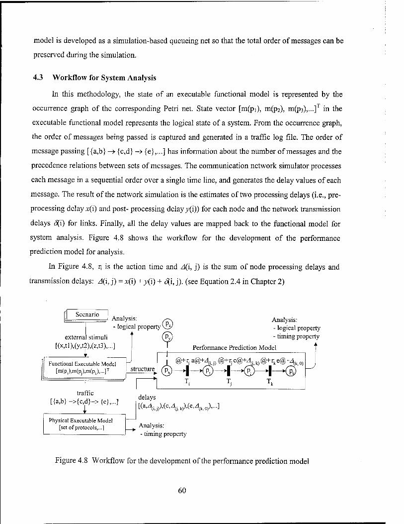
model is developed as a simulation-based queueing net so that the total order of messages can be

preserved during the simulation.

4.3 Workflow for System Analysis

In this methodology, the state of an executable functional model is represented by the

occurrence graph of the corresponding Petri net. State vector [m(pi), m(p2), m(p3),...]T in the

executable functional model represents the logical state of a system. From the occurrence graph,

the order of messages being passed is captured and generated in a traffic log file. The order of

message passing [{a,b} —» {c,d} -» {e},...] has information about the number of messages and the

precedence relations between sets of messages. The communication network simulator processes

each message in a sequential order over a single time line, and generates the delay values of each

message. The result of the network simulation is the estimates of two processing delays (i.e., pre-

processing delay x(i) and post- processing delay y(i)) for each node and the network transmission

delays S(i) for links. Finally, all the delay values are mapped back to the functional model for

system analysis. Figure 4.8 shows the workflow for the development of the performance

prediction model for analysis.

In Figure 4.8, z] is the action time and A(i, j) is the sum of node processing delays and

transmission delays: A(i, j) = x(i) + y(i) + <5(i, j). (see Equation 2.4 in Chapter 2)

Scenario

externa

Analysis: - logical property VI:

stimuli [(x,tl),(y,t2),(z,t3),...]

Functional Executable Model [m(pi),m(pj),m(pk),...]

T

traffic [{a,b} ->{c,d}-> {e},...]

Physical Executable Model [set of protocols,...]

structure

Performance Prediction Model

Analysis: - logical property - timing property

ö+r a(S+4

H—<g)J I >@ »I »S

delays

Ka'4i.jP'(c'zlü,k))'(e'4k,o))'-]

Analysis: - timing property

Figure 4.8 Workflow for the development of the performance prediction model

60

4.4 Procedures to Develop Synthetic Executable Model

The methodology for developing a synthetic executable model for performance prediction

of a real-time distributed system consists of six major steps:

1. Develop basic executable functional model,

2. Identify network service interfaces,

3. Create message dependency relations,

4. Simulate executable physical model,

5. Estimate node processing time and network delays, and

6. Introduce time to basic executable functional model.

4.4.1 Step 1: Develop basic executable functional model

The functional decomposition can be carried to any level of detail. It may depend on the

level of abstraction and modeling purpose. In practical terms, it is carried out to the point that the

lowest level tasks must be executed by a single resource (Levis, 1992). To estimate the network

delays, we need to identify the physical resources in the communication network architecture. So,

the decomposition process may stop at the level at which the physical resources can be identified

at the communication network and its elemental performance parameters are known.

Suppose that the static functional architecture in Figure 3.3 describes a system to be used to

clear threats in which a man-machine decision making system makes decisions to respond to the

threats based on input sensor values. A corresponding Petri net structure can be depicted as

shown in Figure 4.9.

As stated in the previous section, the performance prediction model requires the synthesis

of both functional and physical models. An executable model for performance prediction needs

the allocation of resources (i.e., assets) to functions. Once a set of tasks is represented by

"transitions," the allocation of assets to perform the tasks is represented by tokens at "places."

Places pi 1, pi2, and pi 3 are used for assignment of assets to tasks. Resources Ri; Rj, and Rk are

instances of the assets. These physical resources will have dual roles: one role as computing

devices in the functional architecture and the other role as traffic generators in the physical

architecture.

61

p2 surveillance directive

e*— P6 p3 engagement rule

X tactical picture

pll sensor (R.)

negated threat

pl3 shooter (Rk)

Figure 4.9 An Example of a Basic Executable Functional Model

As a computing device, the physical resource can be interpreted as a server to carry out a

task. Adding these physical resources to the executable functional model denotes that the task

uses the service of the resource to execute the task. If those resources at places pll, pl2, and pl3,

are used only once and consumed, those arcs will be uni-directional arcs from pll to Tj, pl2 to

Tj, and pl3 to Tk. Similarly, if the engagement rule at place p6 is used only once and consumed,

the arc from p6 to Tj will be uni-directional. If the rule is used repeatedly and updated

dynamically, the arc must express a self-loop. If the rule changes dynamically depending on the

state, it must have a time stamp and hence the color set of place p6 must be timed.

62

4.4.2 Step 2: Identify network service interfaces

The communication network simulation model can be generalized as a network of a set of

nodes, namely Ni, N2, ..., Nn, and a set of links which are node pairs (i, j) between node N; and

node Nj. Each link has a capacity Q,-, j), counted in bandwidth units. Links are undirected; (i, j)

and (j, i) denote the same link. These links describe the duplex transmission links of the

communications network. In order to describe the node processing of an information system, a

special link with node pair (x, x) is added as an extension to the transmission link. The capacity

C(x, x) of the special link, then, can be used to specify the node processing rate in bandwidth units.

In this executable physical model, the resources are modeled as part of the network nodes.

As shown in Figure 4.10, the resource Rj, R,, and Rk are added to the communication network as

leaf nodes Nj>, Nj-, and Nk- respectively. The physical resources allocated to the functional

architecture model generate the application network traffic. The same physical resources

connected to a communication network model can be used to identify the communication service

access points in the network.

Figure 4.10 Communication Network Access Points

63

When resource Rx is added to the communication network, the resource node is composed

of two nodes Nx and Nx-, where Nx is the communication service access points and Nx> is an extra

terminal node added to model the special link for representing node processing rate. That is, the

capacity of the special link for the node processing rate is represented by the capacity C(X, X') of

the link (x, x'). In Figure 4.10, the capacities Q, ;>), Qj, J-), and C(k, k') represent the bandwidth of

the information processing rate. In this methodology, the message traffic has seven attributes;

message identification (ID) number, source node, destination node, message size, priority,

protocol, and message dependency relation.

The appearance of tokens m(i, j), m(i, k), m(j, k), m(j, i), and m(k, j) in places p3, p4, p7,

p2, and p5 in Figure 4.9, respectively, represents the message-passing among tasks Tj, Tj, and Tk.

The corresponding source-destination node pairs in the physical model are identified by the

physical node pairs (Nf, Nj), (Nf, Nk), (Nj, Nk), (Nj, Nj), and (Nk, Nj), respectively. The

appearance of tokens in place p6 in Figure 4.9 does not involve the network transmission delay.

The message m(j, j) involves only the node processing time in the information processing system.

The source-destination nodes pair at the physical node is identified by the special link with node

pair (Nj, Nj). Practically, it is implemented by the link with node pair (Nj, Nj>) adding the

additional leaf node Ny.

4.4.3 Step 3: Create message dependency relations

When the firing sequence of transitions is known, we can determine the sequence of

message passing. When the firing sequence is not known, we have to consider all possible

sequences of transitions. All possible sequences are captured in the full occurrence graph of the

Petri net. Generating a full occurrence graph and searching it exhaustively are not practically

acceptable when the state space is large.

In a deterministic Petri net with a conflict free net structure, the firing of one transition

does not disable other transitions. Once tokens in the input places of a transition fulfill the

enabling conditions, the transition will definitely fire. So, even though multiple transitions in a

Petri net are enabled concurrently, the final markings of the net are the same regardless of the

firing order of the concurrently enabled transitions in a deterministic Petri net with a conflict free

net structure. Also, the group of messages that are produced after firing of concurrently enabled

transitions have no precedence relations within them. Message dependency relations occur only

64

between different sets of messages that are produced after subsequent firings other than

concurrent firings. Thus, given a conflict free net with initial markings, one sequence of

occurrence of markings in a partial occurrence graph has all the information necessary to count

the number of messages in the system and their precedence relations. If we generate a partial

occurrence graph using the depth-first search algorithm and there is no circuit in the net, it is not

costly to capture the message dependency relations, and the methodology developed can be used

effectively.

If a Petri net is not conflict free, however, the net may have multiple final markings. Even

if the net has a single final marking, there may exist multiple sequences of occurrences of

markings that have different precedence relations amongst different sets of messages. To handle

those non-conflict free nets, the methodology may require repeated simulations of the

communications network corresponding to the different paths in the full occurrence graph.

One alternative way to estimate network delays between all transitions is to set the initial

marking so that all transitions are covered in each path of the full occurrence graph. Then, the

methodology can estimate the network delay between tasks by selecting one path under the

assumptions that the communications network has the following characteristics: (1) network

delays are longer under heavier traffic loads than under lighter traffic loads, and (2) the degree of

traffic loads is defined as the amount (e.g., number or size) of messages in a given time interval.

By selecting the path that has the maximum number of messages, the methodology can estimate

the upper bound of network delays given the initial marking. Similarly, by selecting the path that

has the minimum number of messages, the methodology can estimate the lower bound of

network delays given the initial marking. Instead of repeated simulations of a communications

network (as many as the number of paths in a full occurrence graph), the alternative method may

be more efficient for a worst-case timing analysis.

The newly generated tokens are identified by subtraction between subsequent markings.

However, the occurrence graph of an ordinary Petri net cannot distinguish the new tokens in a

self-loop. By using a Colored Petri net (see Appendix A) model and by adding a counter at the

self-looped place, we can distinguish them. In a model of a real-time system, new tokens in a

self-loop can be distinguished by their time stamps. So there are two ways for distinguishing new

tokens in a self-loop (a) by adding a logical time stamp, and (b) by using a counter. If we

65

generate an occurrence graph after assigning time delays to transitions, the occurrence graph

becomes a timed occurrence graph. The subtraction operation over the markings of a timed

occurrence graph can distinguish them.

For example, by adding time delay "l"on the arc from transition Tj to place p6 in Figure

4.7, if necessary, we can distinguish the new tokens in the self-loop. Table 4.3 shows the

message dependency relations that were generated from a timed occurrence graph. At each

column of the right side of the table, messages with "+" sign are triggered by messages with the

"-"sign.

The evolution of the state change at the place p6 can now be identified in Table 4.3 while it

was non-identifiable in Table 4.2 (see the bolded cell in both figures). This is necessary

depending on the applications. Suppose that the task Tj is a computerized algorithm and the place

p6 is a rule base. The delay value associated with the self-looped arc between transition Tj and

place p6 may represent the processing or the retrieving time of the rule from the database even

though it has no message transmission delay.

Table 4.3 Subtraction of Marking Vectors from the Timed Occurrence Graph

Whether one uses a counter or a logical

Mo Mi M2 M3 Mi-M0 M2-M1 M3-M2

M(pi) (1,0) (0,0) (0,0) (0,0) -1 0 0

M(p2) (1,0) (0,0) (1,2) (1,2) -1 +1 0

M(p3) (0,0) (1,1) (0,0) (0,0) +1 -1 0

M(p4) (0,0) (1,1) (1,1) (0,0) +1 0 -1

M(p5) (1,0) (1,0) (0,0) (1,3) 0 -1 +1

M(p6) (1,0) (1,0) (1,2) (1,2) 0 ±1 0

M(p7) (0,0) (0,0) (1,2) (0,0) 0 +1 -1

M(p8) (0,0) (0,0) (0,0) (1,3) 0 0 +1

time stamp depends on the applications. The

occurrence graph using the logical time stamp may generate a partial occurrence graph since a

timed occurrence graph is a subset of an untimed occurrence graph (Jensen, 1997). Whether to

use the counter or the logical time stamp depends on the trade-off between having the benefit of

the full occurrence graph and the benefit of the efficiency in generating the partial occurrence

66

graph respectively. In a conflict free net, the order of message passing does not change even

though we use the logical time stamp. So in a conflict free net, we can extract the number of

messages and their precedence relations without affecting the logical behavior.

4.4.4 Step 4: Simulate executable physical model

The role of message dependency (or precedence relations) is to determine the order of

message passing to schedule every message over a single time line during the simulation. Figure

4.11 shows the message dependency graph derived from the timed occurrence graph based on

Table 4.3. At this step, the message attributes: message identification (ID) number, source node,

destination node, message size, priority, protocol, and message dependency relation, are

designated using the information obtained in the previous step. Node ID 0 (No) in the graph

means the external environment.

Table 4.4 is a traffic log in table format representing the message dependency relations.

Instead of having a message generation time, which is usually specified by a probabilistic form

such as Poisson or exponential distribution in a typical communication network simulation

approach, each message is specified by its dependency relations.

Since the delays are not known at the logical model, the time stamp of messages from the

logical model can not be used directly for scheduling. The time stamps of the initial messages are

scheduled at the stamped time in the event list. Table 4.4 shows that messages 1, 2, 3, and 4 are

the initial messages and have no preceding messages. So these four messages are scheduled at the

stamped time on the event list. After that, the messages are ordered by dynamic scheduling as

explained in section 4.1.3.

Figure 4.11 shows that two messages with IDs 5 and 6 will be triggered after two initial

messages with IDs 1 and 2 are processed. If transition T (see Figure 4.9) has an action delay

(e.g., ill), however, messages with IDs 5 and 6 must be generated after the action delay.

Similarly, three messages with IDs 7, 8, and 9 will be triggered after three preceding messages

with IDs 3, 4, and 5 are processed. If transition Tj has an action delay (e.g., xl2), then, messages

with IDs 7, 8, and 9 must be generated after the action delay. In turn, two messages with IDs 10

and 11 will be triggered after two preceding messages with IDs 6 and 9 are processed. If

transition Tk has an action delay (e.g., T13), then, messages with IDs 10 and 11 must be generated

after the action delay.

67

m(ps) - tcp 4 1000 13 0

{6,9} 11 0

m(P7)- tcp 3 1000 12 13

{3,4,5} 9 0

m(P6) udp 1 1

0 12 {} 4 0

tcp 3 1000 12 12

{3,4,5} 8 0

m(p5)-

m(p4)-

udp 1 1 0 12 {} 3 0

\

tcp 2 1000 11 13 1,2} 6 0

protocol timestamp msg_size

source sink

dependency msgid priority

m(p3)

m(p,)-

m(P,)'

/■ V "\^ \

tcp 2 1000 11 12

{1,2} 5 0

tcp 4 100 13 12

{6,9} 10 0 / / f ,' ..\

udp 1 1 0 11 {} 2 0

tcp 3 1000 12 11

{3,4,5} 7 0

udp 1 1 0 11 {} 1 0

Figure 4.11 Message Dependency Graph

Table 4.4 Message Dependency Table

ID Source destination size priority protocol dependency

1: w0(pl) EXTERNAL K lbyte 0 UDP [1 2: /«0(p2) INITIAL Ni lbyte 0 UDP []

3: w0(p5) INITIAL Nj lbyte 0 UDP Ü

4: m0(p6) INITIAL Nj lbyte 0 UDP []

5: w,(p3) N,- N, lOOObyte 0 TCP [1,2]

6: m,(p4) N,- Nk lOOObyte 0 TCP [1,2]

7: w2(p2) Nj Nj lOOObyte 0 TCP [3,4,5]

8: ;«2(p6) N, Nj lOOObyte 0 UDP [3,4,5]

9: m2(p7) Nj Nk lOOObyte 0 TCP [3,4,5]

10: m3(P5) Nk Nj lOOObyte 0 TCP [6,9]

ll:*»3(p8) Nk EXTERNAL lOOObyte 0 UDP [6,9]

68

4.4.5 Step 5: Estimating node processing time and network delays

For each task node i of the executable functional model, the node processing times x(i) and

y(i) are measured using the Equation 4.2. The message processing rate B(i) is the capacity C(i, V)

of the special link with node pair (N„ Nr). The pre-processing time x(i) is measured by the

processing time of the input messages J]«(«,/), where n is the number of input resource nodes n

to the resource node i, and the post-processing time y(i) is measured by the processing time of the

output messages ^/«(/,«), where n is the number of output resource nodes from the resource n

node /.

If multiple messages are competing to use the computing device of the resource i at the

same time , they can be ordered with respect to any criteria since the messages are scheduled

dynamically preserving the total order. In a tactical communication system, the messages often

have a priority or FIFO protocol is used. In Table 4.4, each message has its own priority for

practice. So they will be processed with the designated priority first, then with FIFO protocol.

The processing time will be measured from the time at which each message enters the queue of

the special link to the time at which the message departs the special link after being processed.

Using this mechanism, the contention of information processing device can be represented, when

several tasks compete to use the same computing device of the resource i,

Once the node processing of each message is completed, the network delay of each

message will be measured from the time it departs the processing node (i.e., the time it enters the

communications network) to the time at which it arrives at the destination node. If a message

does not involve the network transmission delay identified by the same node IDs of the source

node and the destination node, the network transmission delay becomes zero. For example, the

place p6 in Figure 4.9 is in a self-loop having the identical source and destination nodes. So the

message with ID 8 does not involve a network delay (i.e., d\i, i) - 0). Similarly, the message with

ID 11 has no network delay because its destination node is the external environment (i.e., d\k, 0)

= 0).

Note that Equation 4.2 produces multiple messages since new tokens are generated by multiple elements (places) of a marking vector and each element (place) can have multiple tokens.

69

The network connection delays can be estimated in two ways: the exact value estimation

approach and the worst-case estimation approach. The exact value estimation approach is to

generate all messages out of the occurrence graph and measure the delay of all messages in a

system. This exact value estimation approach may not be efficient when the system has periodic

information flow. Consider an AAW system with multiple threats. If a sensor observing a target

periodically reports the status of the target, the total number of messages in the system, which are

generated from the occurrence graph, may increase tremendously.

The worst-case estimation approach is to measure the network delay under the assumption

that the communication network characteristics are: (1) network delays are longer under heavier

traffic load than under lighter traffic load, and (2) the degree of traffic load is defined as the

number of messages in a given simulation time such that the traffic load with the same number of

messages in a short simulation time is higher than those in a long simulation time.

Consider that the messages are triggered by the occurrence of the threat. The number of

threats does not change the message-passing pattern assuming that the system does not

dynamically adapt as a function of load. If we figure out the message-passing pattern using a case

with one threat, we can use this pattern repeatedly. We can represent multiple threats using the

inter-arrival time of threats (messages). Suppose the scanning cycle of the sensor is 2 seconds.

This generates a periodic message flow every 2 seconds. But the message pattern does not

change. We can simulate the communication network using the message pattern from a single

threat case with the inter-arrival time of 2 seconds.

Now suppose that, in section 4.4.4, the action times ill (scanning cycle of a sensor), xl2

(decision time of a decision maker), and xl3 (loading time of a missile) can have interval values

depending on the characteristics of resources. Suppose til = [0, 2], T12 = [5, 10], xl3 = [1, 2].

If we use the lower bound action times (i.e., xll =0, T12 = 5, xl3 = 1) for simulation, the

message inter-arrival times are reduced and the traffic becomes denser compared to the case that

we use the upper bound action times (i.e., xll =2, xl2 = 10, xl3 = 2). If we set all the inter-

arrival times to be 0, the resulting network delay, under the assumptions, will represent the

maximum delay value, while the resulting network delay with the upper bound inter-arrival time

will represent the minimum value. So the minimum and maximum action time of a task

70

execution time may be used to estimate the bounded network delays (the minimum and

maximum network delays) under the assumptions.

After measuring the processing time and network delay while running the simulation, two

types of delay information can be obtained. One is the statistical representation of the delay in a

probabilistic form, and the other is a pair of bounded network delays. Assume that the

communications network has the characteristics explained above. If the delays with light traffic

load (lower bound network delays) are smaller than the delays with heavy traffic load (upper

bound network delays), and if they are consistent for various degrees of traffic load, the two

assumptions regarding the characteristics of the communications network may be considered

reasonable. Then, we can determine the minimum and maximum network delay pairs for each

message and use them to verify the end-to-end timing constraints.

4.4.6 Step 6: Introduce time to the basic executable functional model

Once we obtain the node processing time and network delays with either a probabilistic

distribution form or bounded delays, these node processing time and network delay values are

specified as arc expressions of a Petri net. This is the last step to develop the performance

prediction model. The resulting Timed Petri net model has all the information to predict the

performance of the system. If we care only about the end-to-end timing delay, this step is not

necessary since the output data from the executable physical model has the same information.

However, this step helps to analyze the logical behavior and timing behavior together using the

resulting timed occurrence graph.

Suppose that the sub-total delays of the information system, as computed by Equation 2.5,

are A{0t i), 4j, i), A{uj), Aih k), zl(kij), 4jij}, AQ, k), and A{k,0>, associated with each place pi, p2, p3, p4,

p5, p6, p7, and p8, respectively. The performance prediction model (Figure 4.12) can be

completed by adding the time values to the basic executable functional model of Figure 4.9.

71

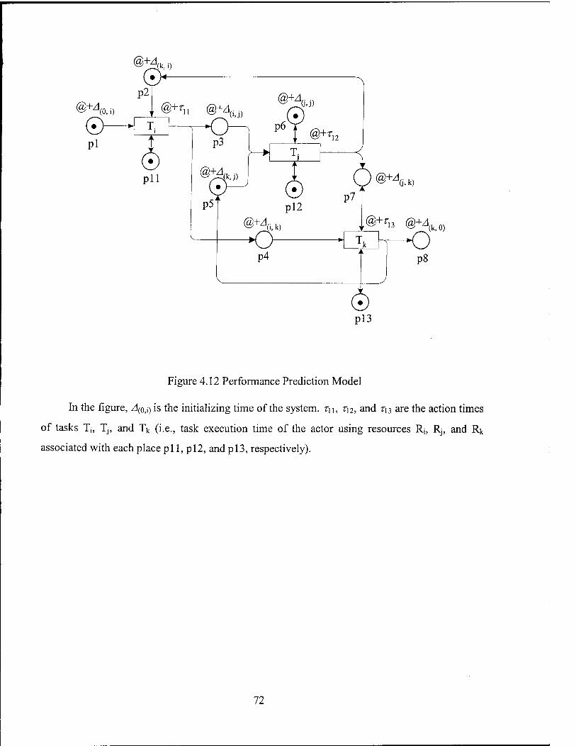
-o p8

6 pl3

Figure 4.12 Performance Prediction Model

In the figure, A(0,i) is the initializing time of the system. T\\, T\I, and r^ are the action times

of tasks Tj, Tj, and Tk (i.e., task execution time of the actor using resources Rj, Rj, and Rk

associated with each place pi 1, pi2, and pi3, respectively).

72

CHAPTER 5. SYNTHETIC EXECUTABLE MODEL GENERATOR

A synthetic executable model generator (SYNE-X) for performance

prediction of a real-time C3 system has been developed so that it can be used

efficiently and effectively for various scenarios or design options. Design/CPN

(1999) has been used for the description of the functional model and Network

Simulator (1999) for the description of the physical model. The SYNE-X consists

of 5 major software components:

Reachability Tree Generator (RTG)

Message Generator (MG)

Performance Prediction Model Converter (PPMC)

Network Topology Generator (NTG)

Communication Network Simulation Script (CNSS)

The four components RTG, MG, PPMC and NTG were implemented using

the ML (Meta Language) imbedded in Design/CPN. CNSS was implemented

using the TCL (Tool Command Language) embedded in Network Simulator.

Figure 5.1 is the detailed workflow model implemented in the Design/CPN

environment. As stated, this dissertation focuses on the synthesis phase of the

system architecting cycle introduced in Section 3.1. The workflow begins with a

functional architecture while a physical architecture is produced at the end of the

analysis phase. Given the basic Petri net model shown in Figure 4.8, the SYNE-X

generates the performance prediction model shown in Figure 4.11. Typically, the

basic Petri net model will be an untimed one. It can be developed as a timed Petri

net model, but with incomplete timing information. The performance prediction

model is the complete timed Petri net model.

73

■ Ghinibu ■

i hrinu 1

f

I Mt IMrill.taM ■■p 1 l' riaddl Lamm nl 'i

< "F*

i 'nnU oh-ppi ail 'i

W

! "FJ i1 nodal■ pmill rt 'i

rV ! "T' ■ ' ntii nihml 'i NIHJ It T^DDnpr I

A ! -^i i* ratti nnftianl '<

A I «^p A i* nutti npmnl 'i

I »Tr I' ratti tapiirn nl ' i

■^wy. * ■ ■pi I Tint* FfrplcUHztal TEL ' i ■■rfvdroA'fMrf XiJmw ■

■ *Uk.i'«ri'MjMpiM',4rc«rir.iiv*i

' JmtifV*!*

«F» I'niiUiAinniri 'i ■■rid v a™'|jci^.V '

■rJ^Tinmi llnlNKMiitl^^

JhYifMBKri-JTMnaita.- | iff/at ■ J T*l l^ JViJW.I |P

■ fT+^QMiMTi ■) CVradii« Imnolfcirum! "j

+ A t 'luAAiipnvnl f £"muKluUi cab do Mt wrf "i

Figure 5.1 Detailed Workflow Model for System Analysis

To describe each step, the same AAW system shown in Figure 4.8 will be used. Figure 5.2

is the basic Petri net model developed in Design/CPN corresponding to Figure 4.8. Table 5.1 is

the declaration of the variables (global declaration node). See Appendix B for an explanation of

the net descriptions implemented by Design/CPN.

74

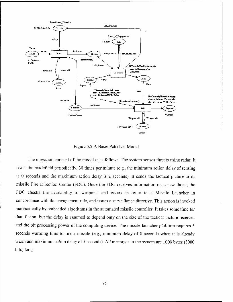
Su tv u 11 »cv_H ma > L

itaLjL-fcjitfli

thui i4-lirfiusi.PiaiLui1widi

Figure 5.2 A Basic Petri Net Model

The operation concept of the model is as follows. The system senses threats using radar. It

scans the battlefield periodically, 30 times per minute (e.g., the minimum action delay of sensing

is 0 seconds and the maximum action delay is 2 seconds). It sends the tactical picture to its

missile Fire Direction Center (FDC). Once the FDC receives information on a new threat, the

FDC checks the availability of weapons, and issues an order to a Missile Launcher in

concordance with the engagement rule, and issues a surveillance directive. This action is invoked

automatically by embedded algorithms in the automated missile controller. It takes some time for

data fusion, but the delay is assumed to depend only on the size of the tactical picture received

and the bit processing power of the computing device. The missile launcher platform requires 5

seconds warming time to fire a missile (e.g., minimum delay of 0 seconds when it is already

warm and maximum action delay of 5 seconds). All messages in the system are 1000 bytes (8000

bits) long.

75

Table 5.1 Global Declaration Node

(* simple AAW model Global Declaration Node *)

color RealCS = int; color Identification = RealCS ; color Counter = int; color TgtID = int timed; color SensorlD = int timed; color WeaponID = int timed; color Threat = product TgtID * Identification; color Asset = union Sensor:SensorlD + Weapon:WeaponID; color TacticalPicture = product SensorlD * Threat; color ScanModes = with Default | TrackingOnlyFor | ScaningOnlyFor ; color SurveillanceDirective = product SensorlD * ScanModes * TgtID; color RulesofEngagement = product RealCS * Counter timed; color Decision = with Fire | WithDraw | Wait; color Order = product TgtID * Decision; color Assessment = with Cleared | KillSelf | Misshit | Leak ; color Negated = product TgtID * Assessment * WeaponID; color Report = Negated;

var dth: RealCS; var counter: Counter; var threat: Threat; var sid: SensorlD; var wid: WeaponID; var rule_s : Surveillance_Directive ; var task: Order;

fun ThreatlsHostile (threat:Threat, dth:RealCS) = #2(threat) > dth; fun Correctlyldentified (threat:Threat) = #2(threat) = 100;

5.1 Stepl: Generating network topology

The network topology is generated by Network Topology Generator (NTG). Figure 5.3 is

an example of a network topology drawn by NTG. NTG provides the user with a GUI to enter the

number of nodes and their attributes; the number of switching (with the circle symbol) and the

number of terminal nodes (with the square box symbol) which are the physical resources

connected to the net. It automatically lays out the nodes in a two-dimensional grid and connects

them in a default network topology of tactical communication networks.

Figure 5.3 shows the nine switching nodes (X_0 to X_8) and four terminal nodes (SI01,

W101, FDQ andAWACS). The bandwidth of all links is 1.024 Mbps with the propagation delay

of 10ms and the queue type of DropTail. The bandwidth between switching node and terminal

76

node is 56Kbps with propagation delay of 10ms and queue type of DropTail. Also, the figure

shows that every terminal node has bit processing power of 66Mbps. This is the bandwidth of the

special link that represents the node processing rate of the information system.

Figure 5.3 An Example of Network Topology drawn by NTG

Once the physical architectures are specified, NTG generates a text file of the network

topology in a specific format so that it can be used by the CNSS. Table 5.2 is an example of the

traffic log file in TCL script format.

5.2 Step2: Mapping physical resources to transitions

The process of selecting alternative resources is an issue of resource allocation or an issue

of physical design to implement the logical functions and it depends on the scenarios. The

mapping between transition and resource is done by NTG and MG. The main use of NTG is to

allow the user to select the physical resources interactively.

77

Table 5.2 Network Topology File

# wan nodes list set caesar_wan_nodes { AWACS W101 S101 FDC X_2 X_8 X_6 X_0 X_5 X_7 X_l X_4 X_3 } # Ian nodes list

set caesar_lan_nodes { } # links in simplex

set caesar_links { {X_0 AWACS} 56Kb 10ms DropTail} {AWACS X_0} 56Kb 10ms DropTail} {X_3 W101} 56Kb 10ms DropTail} {W101 X_3} 56Kb 10ms DropTail} {W101 X_4} 56Kb 10ms DropTail} {X_4 W101} 56Kb 10ms DropTail} {X_4 SI01} 56Kb 10ms DropTail} {SI01 X_4} 56Kb 10ms DropTail} {S101 X_l} 56Kb 10ms DropTail} {X_l S101} 56Kb 10ms DropTail} {FDC X_4} 56Kb 10ms DropTail} {X_4 FDC} 56Kb 10ms DropTail} {FDC X_8} 56Kb 10ms DropTail} {X_8 FDC} 56Kb 10ms DropTail} {X_0X_3} 1.024Mb 10ms DropTail} {X_3 X_6} 1.024Mb 10ms DropTail} {X_6X_7} 1.024Mb 10ms DropTail} {X_7X_8} 1.024Mb 10ms DropTail} {X_8 X_5} 1.024Mb 10ms DropTail} {X_5 X_2} 1.024Mb 10ms DropTail} {X_2 X_l} 1.024Mb 10ms DropTail} {X_l X_0} 1.024Mb 10ms DropTail} {X_0X_1} 1.024Mb 10ms DropTail} {X_l X_2} 1.024Mb 10ms DropTail} {X_2 X_5} 1.024Mb 10ms DropTail} X_5 X_8} 1.024Mb 10ms DropTail} X_8 X_7} 1.024Mb 10ms DropTail}

{X_7 X_6} 1.024Mb 10ms DropTail} {X_6X_3} 1.024Mb 10ms DropTail} {X_3 X_0} 1.024Mb 10ms DropTail} {X_3 X_4} 1.024Mb 10ms DropTail} {X_4X_5} 1.024Mb 10ms DropTail} {X_5 X_4} 1.024Mb 10ms DropTail} {X_4 X_7} 1.024Mb 10ms DropTail} {X_7X_4} 1.024Mb 10ms DropTail} {X_4X_1} 1.024Mb 10ms DropTail} {X_l X_4} 1.024Mb 10ms DropTail} {X_4 X_3} 1.024Mb 10ms DropTail}

78

MG allows the user to allocate resources in order to generate the source and destination

nodes of the communication network. NTG and MG provide the user with a Graphic User

Interface (GUI) developed in the Design/CPN environment in order to obtain information

necessary to produce the traffic log file. This GUI helps to select instances of resources that are

connected to the communication network as leaf nodes. The specification of the physical

resources has two attributes: the name of the asset and the action time when the actor executes

the task (transition) using the asset. Figure 5.4 shows the specification at a dotted square box.

MG also allows the user to enter the attributes of actors. This action time is differentiated

from the node processing delay and network transmission delays. The delay of an actor is

associated with the delay of the task executor(s). If every task is an autonomous data processing

task, the actor's delay may be set to "0". Once this attribute is obtained, it is maintained at a

special region of each transition.

ll»o_E<uxii>u

.X. l-tCU.CkfÄi/rdl (_ Hii=i«;J>* lUHJOk.-bi|[0l

if I Gnuxd^Umi-riuJ ihiisi diui i#üdiusi£lumi2i,widi iJn:i*bdiiL>i.}:llädf»idi

Wopcrt wid

Figure 5.4 Mapping Resources to Transition

79

5.3 Step 3: Checking the syntax of the basic Petri net model

This step is supported by RTG. The SYNE-X was designed to import any Petri net model

once it is developed in Design/CPN. It uses the Occurrence Graph Analyzer, which is a

component of Design/CPN, to capture the order of message-passing. Design/CPN has a built-in

syntax checker. RTG allows the user to fix the imported model to be compliant with the syntax

ofOGA.

5.4 Step 4: Generating an Occurrence Graph

The RTG primarily uses the software function codes provided by the OGA of Design/CPN.

However, this component was implemented to be interactive with users. It generates a

reachability tree, searches final states, and calculates the shortest and longest paths from the

initial state to final states. RTG generates a partial reachability tree until it finds at least one final

state. Figure 5.5 is the full OG of the basic Petri net model generated by RTG.

If the net is conflict free, this partial reachability tree can be used to capture all the

necessary state information. If the net is not conflict free, the user will be provided an option to

search all final states and select one of the paths from the initial state to multiple states. The

example model is a conflict free net. Any path in the occurrence graph can capture the order of

events.

Table 5.3 is the list of newly generated tokens derived from the sequence of markings Ml-

M3-M5-M7-M10-M11. From Table 5.3, we can identify which tokens ("MessageJD") are

generated from which transition ("FiredJTransition") to which place ("Place Instance"). Table

5.4 is the list of triggering tokens derived from the same sequence of markings.

The major role of RTG is to capture the precedence relations between tokens (i.e.,

messages). From the causal relation between tokens on the two tables, we can identify the total

order of message-passing.

5.5 Step 5: Developing an intermediate Timed Petri net model

This step is supported by PPMC. The main purpose of the Performance Prediction Model

Converter is to transform the basic Petri net into a Timed Petri net (i.e., Performance Prediction

Model). An example of the transformed Timed Petri net model is shown in Figure 5.6.

80

■■1MB Min J

■ MM ■■■■■■ J J V<««UMJl|p

IBM MMAT J J MJ JnÜM ■■■]■! J

IJ

■r^JM*« J j»" ■MMBMPK J J VJ1

•mirm J , *1l"l 1 1«.. ■far«***- J iMjarfaa j J IJU u ■• a]|a|

!■§■ ■TBMM J J ■m — ■•■1-1 1 !:: mrmdm? J U MI«]|B|

i^_ ■in J IHM "I*" l —™ ■MiaMra j i »^i

U JM 1l-f > 1 '■«4» -><PI 1

J IJtU

■■raarir- ■■

1 ■ J

!-- ■am j

as:; . ■*■*■ uuiqp, . mmrm j |~H ■Air«*«- j ■ M^daa j J IJU u «■■■4Pn J 11 u ■ ■ll-l

i"*"" «■an j j ■TBBBi !■■ wamdif j 4 ijy

■■■r J J ■

■ ■■ ■in j j J aamr 4I*I j ■f^M-a J

l = = ■MlBMPfl J J ■■■rw j

«^■IUUI^I .

M.«MIM J u Julian J IJBJ U ■■ ■.I"!

mm nBMi j j VWBMl -■«■l"i j — -J-r J

Figure 5.5 Full Occurrence Graph from Basic Petri Net (Untimed)

Table 5.3 List of Newly Generated Tokens

*** New Messages Generated at Each Occurrence of Marking of model: simpleAAW *** Marking_No Fired_Transition Binding Place Instance with List of Tapped (Msg_ID, Marking, Time_Stamp)

Mi_l INITIAL INITIAL IADS'Threat 1 (1,(1,100),0.0) (2,(2,0),0.0) IADS'Rule 1 (3,(90,0),0.0) IADS'Directive 1 (4,(101,Default,0),0.0) IADS'Sensor 1 (5,Sensor(101),0.0) IADS'Shooter 1 (6,Weapon(101),0.0)

Mi_3 IADS'Sense 1 IADS'Sense 1: {threat=(l,100),sid=101,mle_s=(101,Default,0)} IADS'Identity 1 (7,(101,(1,100)),0.0) IADS'Location 1 (8,(101,(1,100)),0.0)

Mi_5 IADS'Command 1 IADS'Command 1: {threat=(l,100),sid=101,dth=90,counter=0} IADS'Order 1 (9,(l,Fire),0.0)

81

IADS'Rule 1 (10,(90,1),0.0) IADS'Directive 1 (ll,(101,Default,0),0.0)

Mi_7 IADS'Actl IADS'Act 1: {wid=101,threat=(l,100),task=(l,Fire),sid=101} IADS'Negated 1 (12,(l,Cleared,101),0.0) IADS'Report 1 (13,(l,Cleared,101),0.0)

MilO IADS'Sense 1 IADS'Sense 1: {threat=(2,0),sid=101,rule_s=(101,Default,0)} IADS'Identity 1 (14,(101,(2,0)),0.0) IADS'Location 1 (15,(101,(2,0)),0.0)

Mill IADS'Command 1 IADS'Command 1: {threat=(2,0),sid=101,dth=90,counter=l} IADS'Rule 1 (16,(90,2),0.0) IADS'Directive 1 (17,(101,Default,0),0.0)

Table 5.4 List of Triggering Tokens

*** Old Messages Removed at Each Occurrence of Marking of model: simpleAAW *** Marking_No Fired_Transition Binding Place Instance with List of Tapped (Msg_ID, Marking, Time_Stamp)

Mi_l INITIAL INITIAL

Mi_3 IADS'Sense 1 IADS'Sense 1: {threat=(l,100),sid=101,rule_s=(101,Default,0)} IADS'Threat 1 (1,(1,100),0.0) IADS'Directive 1 (4,(101,Default,0),0.0)

Mi_5 IADS'Command 1 IADS'Command 1: {threat=(l,100),sid=101,dth=90,counter=0} IADS'Identity 1 (7,(101,(1,100)),0.0) IADS'Rule 1 (3,(90,0),0.0)

Mi_7 IADS'Actl IADS'Actl: {wid=101,threat=(l,100),task=(l,Fire),sid=101} IADS'Location 1 (8,(101,(1,100)),0.0) IADS'Order 1 (9,(l,Fire),0.0)

Mi_10 IADS'Sense 1 IADS'Sense 1: {threat=(2,0),sid=101,rule_s=(101,Default,0)} IADS'Threat 1 (2,(2,0),0.0) IADS'Directive 1 (ll,(101,Default,0),0.0)

Mi_ll IADS'Command 1 IADS'Command 1: {threat=(2,0),sid=101,dth=90,counter=l} IADS'Identity 1 (14,(101,(2,0)),0.0) IADS'Rule 1 (10,(90,1),0.0)

82

np^ Liui_. n.-<iiL_ib. ■(■. ni

nrirf L-im/c—i.n.-dx^.c«- Hi

pan** i^m.'.i«_i M[ixn) Map* lim.'.iM_ll^axllilinMlnCn^

^■■daribiiiH ■_-■ i i

JI M lpt1 art I HI fcM3wl*di« Li I1XT* MMMMI _ I* li CO/D M ■ w 4 bl i|0*ita ifcttfcl ■ nl^air I. f

|aifl.A4Lh IIHMI

i-t*—*infmi T.-Qi|,^i^a»-T,-<fi|

da Hli__i>Jllat^_l M«_IB1.T.4> 4 H*i>IMi.T^p \ I

wäoi;

Figure 5.6 Intermediate Performance Prediction Model

Compare the transformed intermediate Timed Petri net model (Figure 5.6) to the basic Petri

net model (Figure 5.1). Figure 5.6, additionally, has a local declaration node, a time delay arc

expression, a code segment, and a temporary declaration node.

The local declaration node defines the variables that represent delay values. Each variable

name specifies a logical connection link name between two tasks. It consists of a transition name

(source) and a place name (sink). Table 5.5 is an example of the local declaration node.

Table 5.5 Local Declaration Node

(* Local Declaration Node *)

pageref IADS'Sensel = [7,14,8,15]; pageref IADS'SenseJ'IADS'Identity = [7,14]; pageref IADS'SenseJ'IADS'Location = [8,15];

pageref IADS'Commandl = [9,10,16,11,17]; pageref IADS'Command 1'IADS'Order = [9];

83

pageref IADS'Command_l'IADS'Rule = [10,16]; pageref IADS'Commandl'IADS'Directive = [11,17];

pageref IADS'AcM = [12,13]; pageref IADS'ActJ'IADS'Negated = [12]; pageref IADS'ActJ'IADS'Report = [13];

The variable name "IADS 'command_l 'IADS 'order" means that the first instance of

transition "command" at the "IADS" page sends messages to place "order" at the "IADS" page.

Those integer values assigned to each variable are message identification numbers. So the total

number of messages in a link represents the total number of newly created messages. For

example, the transition "command" generated 5 tokens (i.e., message ID 9,10,16,11,and 17) and

the place "order" received one token (message ID [9]), and the places "Rule" and "Directive"

received two tokens (message IDs [10,16] and [11,17] respectively) each from the transition

"command". The values of the delay variables at the local declaration node shall be replaced by

the estimated ones at the final step.

The delay variables are automatically added at the tail of each arc expression with a time

expression. The "fnDELTA" on an arc expression is the delay selection function. If a time delay

expression appears on an arc, the arc's ending place must be declared as a timed color set.

The delay variables of the local declaration node and the delay variables of arcs are mapped

in the code segment. Table 5.6 is an example of the code segment.

Table 5.6 Code Segment

output (d3,d2,dl,bl); action let val

d3 = getDelayNet MinOrMaxNet IADS'Command 1'IADS'Directive and d2 = getDelayNet MinOrMaxNet IADS'Command 1'IADS'Rule and dl = getDelayNet MinOrMaxNet IADS'CommandJ'IADS'Order and bl = getDelayBase MinOrMaxBase IADS'Command 1

in(d3,d2,dl,bl)end;

In the code segment, another two delay retrieving functions are used with names

"getDelayBase" and "getDelayNet". These are used to retrieve the delay values from the local

declaration node and send them to each arc. The function "getDelayBase" retrieves the pre-

84

processing time (plus the action time and the post processing time, depending on the application)

while the function "getDelayNet" retrieves the transmission delay (and the post processing time,

depending on the application). The base delay is the common delay of all arcs and the net delay is

only applied to the specific arc. Depending on the application, the user may consider the post

processing as the delay value of the arc. The difference of the two types of delay shall be

considered when the delay values are introduced at the last step 9.

The functions associated with delays (i.e., getDelayBase, getDelayNet, and fnDELTA) are

defined at the temporary declaration node (Table 5.7). These functions can be also defined as

user's preference. By default, they were defined to get the minimum delay, maximum delay, zero

delay, and random delays. The user can select this option anytime during simulation of the Petri

net.

Table 5.7 Temporary Declaration Node

(* Temporary Declation Node *)

exception TimeNotDetermined ; globref TIMESCALE = 1000000.0; globref MinOrMaxBase = "Max"; globref MinOrMaxNet = "Max";

vard3,d2,dl,bl : TIME ; val DelayUnit = "real"; val DELAYJNSEC = 1;

fun D2Sec (d:int) = Intlnf.fromlnt (d * DELAY_IN_SEC); fun R2Time (r:real) = Option.valOf (Intlnf.fromString (Real.toString (r * (ITIMESCALE)))); fun I2Time (i:lntlnf.int) =

let val r = (Option.valOf (Real.fromStiing (Intlnf.toString i)));

in R2Time r end;

fun Time2R (i:lntlnf.int) = (Option.valOf (Real.fromString (Intlnf.toString i))) /(ITIMESCALE)

fun defmeDelayUnitlnLocaDecNode () = if DelayUnit = "int" then usestring ["fun Delay2Time (ID:int)= Intlnf.fromlnt ID;val DELAYJJNIT = 0;"]

else usestring ["val Delay2Time = R2Time;val DELAYJJNIT = 0.0;"]; defineDelayUnit_InLocaDecNode ();

fun ZeroDelay (xs) = DELAYUNIT;

fun AvgDelay (xs) = let fun sum nil = DELAY_UNIT

| sum (x::xs) = x + sum(xs) in (sum xs) / (real (length xs)) end;

85

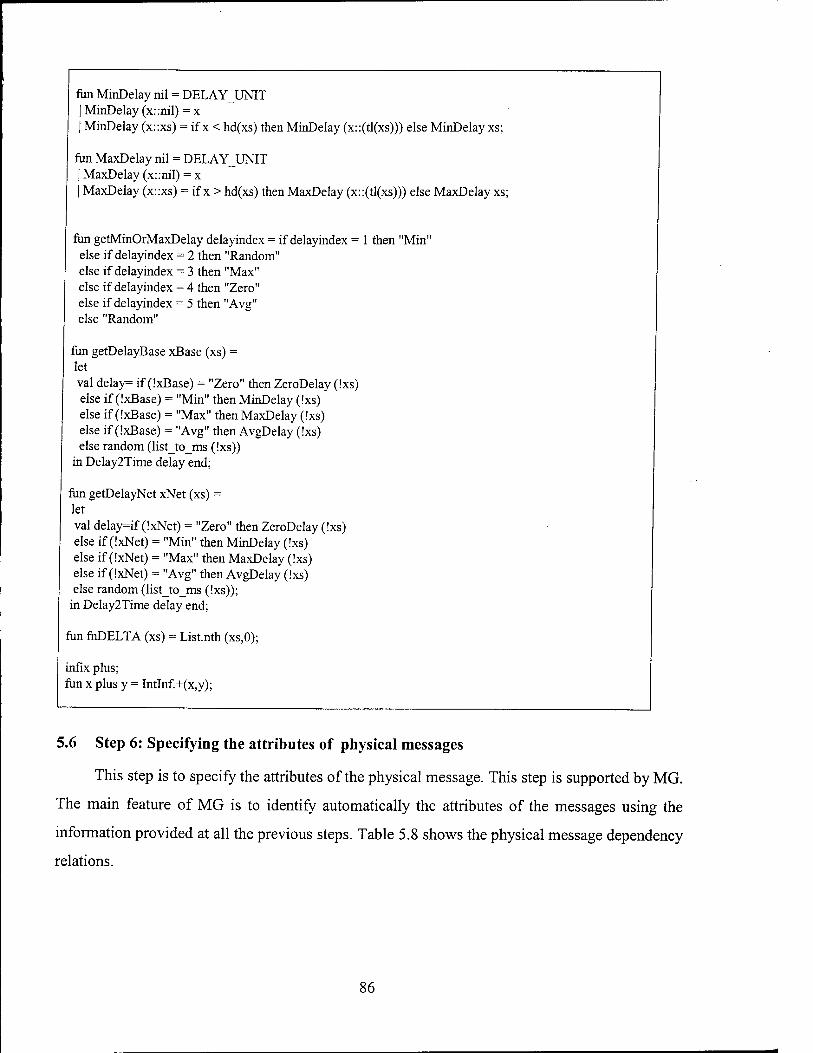
fun MinDelay nil = DELAYUNIT |MinDelay(x::nil) = x | MinDelay (x::xs) = if x < hd(xs) then MinDelay (x::(tl(xs))) else MinDelay xs;

fun MaxDelay nil = DELAYJJNIT | MaxDelay (x::nil) = x | MaxDelay (x::xs) = if x > hd(xs) then MaxDelay (x::(tl(xs))) else MaxDelay xs;

fun getMinOrMaxDelay delayindex = if delayindex = 1 then "Min" else if delayindex = 2 then "Random" else if delayindex = 3 then "Max" else if delayindex = 4 then "Zero" else if delayindex = 5 then "Avg" else "Random"

fun getDelayBase xBase (xs) = let val delay= if (IxBase) = "Zero" then ZeroDelay (!xs) else if (IxBase) = "Min" then MinDelay (!xs) else if (IxBase) = "Max" then MaxDelay (!xs) else if (IxBase) = "Avg" then AvgDelay (!xs) else random (list_to_ms (!xs))

in Delay2Time delay end;

fun getDelayNet xNet (xs) = let val delay=if (IxNet) = "Zero" then ZeroDelay (Ixs) else if (IxNet) = "Min" then MinDelay (Ixs) else if (IxNet) = "Max" then MaxDelay (Ixs) else if (IxNet) = "Avg" then AvgDelay (Ixs) else random (list_to_ms (Ixs));

in Delay2Time delay end;

fun fnDELTA (xs) = List.nth (xs,0);

infix plus; fun x plus y = Intlnf.+(x,y);

5.6 Step 6: Specifying the attributes of physical messages

This step is to specify the attributes of the physical message. This step is supported by MG.

The main feature of MG is to identify automatically the attributes of the messages using the

information provided at all the previous steps. Table 5.8 shows the physical message dependency

relations.

86

Table 5.8 Message Dependency Relations

(* Traffic Specification *)

val LinkSpec = [

{link="INITIAL'IADS'Sense_l", src="INITIAL", dest="S101", delay="[0,0]", proc="8", protocol="UDP", size="l", priority="0", msgs=[ 1,2,4]},

{link="INITIAL'IADS'Command_l", src="INITIAL", dest="FDC", delay="[0,0]", proc="8", protocol="UDP", size="l", priority="0", msgs=[3]},

{link="IADS'Sense_l'IADS'Command_l", src="S101", dest="FDC", delays"[0,2]", proc="66Mb", protocol="TCP", size="1000", priority="0", msgs=[7,14]},

{link="IADS'Sense_l'IADSAct_l", src="S101", dest="W101", delay="[0,2]", proc="66Mb", protocol="TCP", size="1000", priority="0", msgs=[8]},

{link="IADS'Sense_rEXTERNAL", src="S101", dest="EXTERNAL", delay="[0,2]", proc="66Mb" protocol="UDP", size="1000", priority="0", msgs=[15]},

{link="IADS'Command_l'IADSAct_l", src="FDC", dest="W101", delay="[0,0]", proc="66Mb", protocol="TCP", size="1000", priority="0", msgs=[9]},

{link="IADS'Command_l'IADS'Command_l", src="FDC", dest="FDC", delay="[0,0]", proc="66Mb", protocol="UDP", size="1000", priority="0", msgs=[10]},

{link="IADS'Command_l'IADS'Sense_l", src="FDC", dest="S101", delay="[0,0]", proc="66Mb", protocol="TCP", size="1000", priority="0", msgs=[l 1]},

{link="IADS'Command_l'EXTERNAL", src="FDC", dest="EXTEPvNAL", delay="[0,0]", proc="66Mb", protocol="UDP", size="1000", priority="0", msgs=[16,17]},

{link="IADSAct_l'EXTERNAL", src="W101", dest="EXTERNAL", delay="[0,5]", proc="66Mb", protocol="UDP", size="1000", priority="0", msgs=[12,13]}

];

MG automatically identifies the logical link (transition to place pair), the physical link

(source -destination node pair), the action time of the task execution, the node processing rate of

the physical information system, and the dependency of messages. In addition to the automatic

identification of the attributes, it allows the user to enter the protocol, size, and priority of the

message for transmission.

5.7 Step 7: Generating the traffic log file

Once MG captures all the attributes of messages, it generates a traffic log file in a specific

format so that it can be used by the CNSS. Table 5.9 is the example of the traffic log file in TCL

script format.

87

Table 5.9 Traffic Log File

set modelname simpleAAW set orig_no_msg 17

#ID src dest size Protocol Priority ProcRate ActionDelay TrglDs Tstamp

set caesar_msgs { {1 INITIAL S101 1 Agent/UDP 0 8 {0 0} {} 0.0} {2 INITIAL S101 1 Agent/UDP 0 8 {0 0} {} 0.0} {4 INITIAL S101 1 Agent/UDP 0 8 {0 0} {} 0.0} {3 INITIAL FDC 1 Agent/UDP 0 8 {0 0} {} 0.0} {5 INITIAL EXTERNAL 1 Agent/UDP 0 8 {0 0} {} 0.0} {6 INITIAL EXTERNAL 1 Agent/UDP 0 8 {0 0} {} 0.0} {7 S101 FDC 1000 Agent/TCP 0 66Mb {0 2} {1 4} 0.0} {14 S101 FDC 1000 Agent/TCP 0 66Mb {0 2} {2 11} 0.0} {8 S101 W101 1000 Agent/TCP 0 66Mb {0 2} {1 4} 0.0} {15 S101 EXTERNAL 1000 Agent/UDP 0 66Mb {0 2} {2 11} 0.0} {9 FDC W101 1000 Agent/TCP 0 66Mb {0 0} {7 3} 0.0} {10 FDC FDC 1000 Agent/UDP 0 66Mb {0 0} {7 3} 0.0} {11FDCS101 1000 Agent/TCP 0 66Mb {0 0} {7 3} 0.0} {16 FDC EXTERNAL 1000 Agent/UDP 0 66Mb {0 0} {14 10} 0.0} {17 FDC EXTERNAL 1000 Agent/UDP 0 66Mb {0 0} {14 10} 0.0} {12 W101 EXTERNAL 1000 Agent/UDP 0 66Mb {0 5} {8 9} 0.0} {13 W101 EXTERNAL 1000 Agent/UDP 0 66Mb {0 5} {8 9} 0.0} I

5.8 Step 8: Simulating the communications network

This step is done by CNSS. NS provides an object-oriented, event-driven simulation engine

with various protocol modules. Figure 5.7 is a communication network simulation model

implemented by Network Simulator.

The nodes with the circle symbol in Figure 5.7 represent the communication nodes and

those with the hexagon symbol represent the information processing nodes. The shaded bars on

each link represent the message flow over the links for emulation.

88

Figure 5.7 Network Simulation (Emulation)

The developed methodology and tools support description of 3 types of delay: Node

processing delay (pre- and post- processing delays) of the computing device, action delay of the

task executor, and transmission delay of the network.

The node processing time describes two types of data processing delays: pre-processing

delay and post-processing delay. The pre-processing delay is a delay between the time at which

all conditioned information arrives and the time at which the task starts execution (e.g., the

decision making process starts). The processing node estimates the data processing time of

incoming data. Assume that sensor A reports data in the form of a large image with the features

of a detected object and sensor B reports data for a small signal regarding the location of the

object. The time to display the information to the decision maker will vary. Some application

89

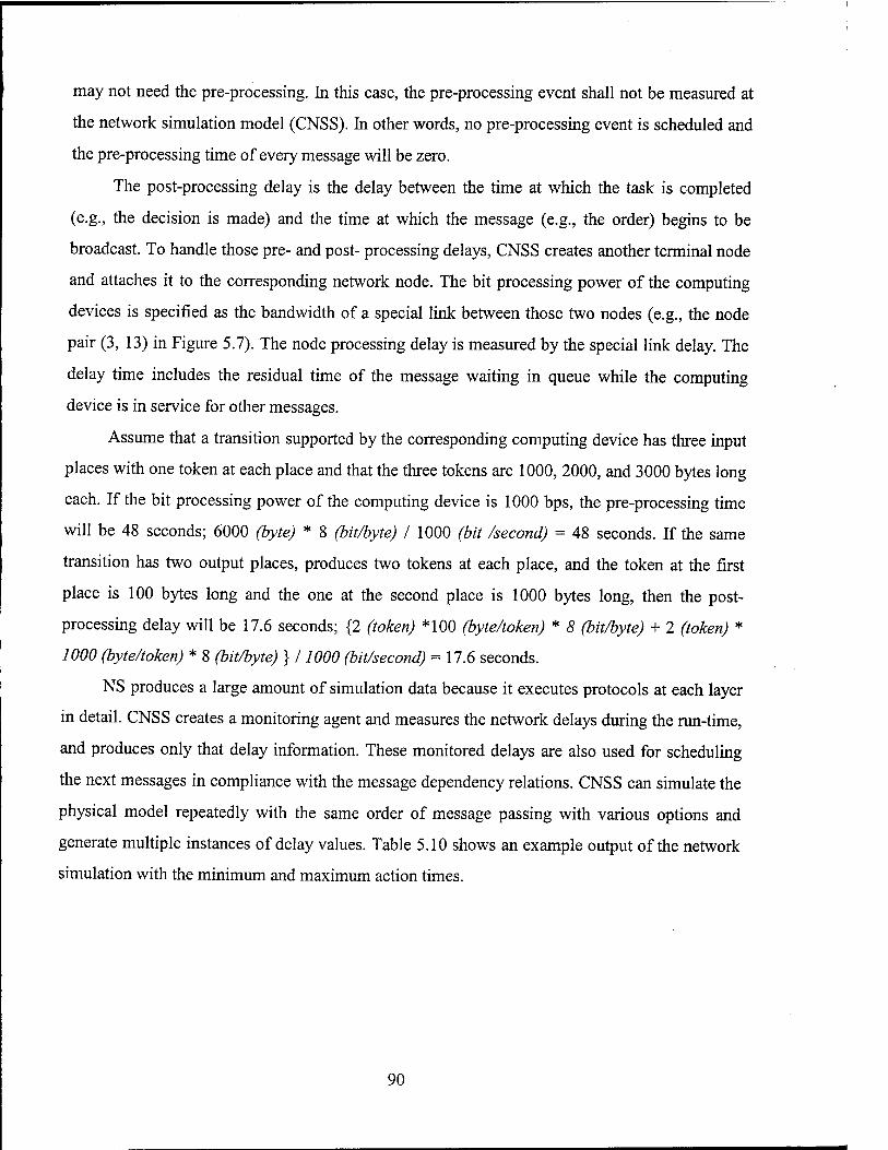
may not need the pre-processing. In this case, the pre-processing event shall not be measured at

the network simulation model (CNSS). In other words, no pre-processing event is scheduled and

the pre-processing time of every message will be zero.

The post-processing delay is the delay between the time at which the task is completed

(e.g., the decision is made) and the time at which the message (e.g., the order) begins to be

broadcast. To handle those pre- and post- processing delays, CNSS creates another terminal node

and attaches it to the corresponding network node. The bit processing power of the computing

devices is specified as the bandwidth of a special link between those two nodes (e.g., the node

pair (3, 13) in Figure 5.7). The node processing delay is measured by the special link delay. The

delay time includes the residual time of the message waiting in queue while the computing

device is in service for other messages.

Assume that a transition supported by the corresponding computing device has three input

places with one token at each place and that the three tokens are 1000, 2000, and 3000 bytes long

each. If the bit processing power of the computing device is 1000 bps, the pre-processing time

will be 48 seconds; 6000 (byte) * 8 (bit/byte) I 1000 (bit /second) = 48 seconds. If the same

transition has two output places, produces two tokens at each place, and the token at the first

place is 100 bytes long and the one at the second place is 1000 bytes long, then the post-

processing delay will be 17.6 seconds; {2 (token) *100 (byte/token) * 8 (bit/byte) + 2 (token) *

WOO (byte/token) * 8 (bit/byte) } / 1000 (bit/second) = 17.6 seconds.

NS produces a large amount of simulation data because it executes protocols at each layer

in detail. CNSS creates a monitoring agent and measures the network delays during the run-time,

and produces only that delay information. These monitored delays are also used for scheduling

the next messages in compliance with the message dependency relations. CNSS can simulate the

physical model repeatedly with the same order of message passing with various options and

generate multiple instances of delay values. Table 5.10 shows an example output of the network

simulation with the minimum and maximum action times.

90

Table 5.10 Delay Values of Messages (simulation with min and max action time)

model name: /simpleAAW/ Number of Origial message: 111 I Number of Processed message: 111 I variables: /("msg_id", ["pre_proc_delay", "action_time","post_proc_delay", "net_delay"])/

(1 ,[0.000000,0.000000,0.000000,0.000000]) (2,[0.000000,0.000000,0.000000,0.000000]) (3,[0.000000,0.000000,0.000000,0.000000]) (4,[0.000000,0.000000,0.000000,0.000000]) (5,[0.000000,0.000000,0.000000,0.000000]) (6,[0.000000,0.000000,0.000000,0.000000]) (7,[0.000000,2.000000,0.000145,0.334274]) (8,[0.000000,2.000000,0.000267,0.477009]) (9,[0.000121,0.000000,0.000122,0.311312]) (10,[0.000121,0.000000,0.000243,0.000000]) (11,[0.000121,0.000000,0.000364,0.453927]) (12,[0.000242,5.000000,0.000121,0.000000]) (13,[0.000242,5.000000,0.000243,0.000000]) (14,[0.000121,2.000000,0.000121,0.305836]) (15,[0.000121,2.000000,0.000243,0.000000]) (16,[0.000242,0.000000,0.000243,0.000000]) (17,[0.000242,0.000000,0.000122,0.000000])

(1 ,[0.000000,0.000000,0.000000,0.000000]) (2,[0.000000,0.000000,0.000000,0.000000]) (3,[0.000000,0.000000,0.000000,0.000000]) (4,[0.000000,0.000000,0.000000,0.000000]) (5,[0.000000,0.000000,0.000000,0.000000]) (6,[0.000000,0.000000,0.000000,0.000000]) (7,[0.000000,0.000000,0.000145,0.334274]) (8,[0.000000,0.000000,0.000267,0.477009]) (9,[0.000121,0.000000,0.000122,0.311312]) (10,[0.000121,0.000000,0.000243,0.000000]) (11,[0.000121,0.000000,0.000364,0.453927]) (12,[0.000242,0.000000,0.000121,0.000000]) (13,[0.000242,0.000000,0.000243,0.000000]) (14,[0.000121,0.000000,0.000121,0.311312]) (15,[0.000121,0.000000,0.000243,0.000000]) (16,[0.000243,0.000000,0.000242,0.000000]) (17,[0.000243,0.000000,0.000121,0.000000])

91

5.9 Step 9: Introducing time to the basic Petri net model

This step maps the delay variables of the local declaration node to the estimated delay

values. Once the delay values are obtained from the physical model, the message IDs are replaced

with their delay values. Figure 5.8 shows the final performance prediction model of the example.

The delay values were imported into the Timed Petri net model as a list of values.

t'-lir-Alard llwctxxx n Lltzfc-Ait-ibiin ad bl3T ni r^ruim u'nv N

flirt, Lac* Uvcixxk nlladm- ■Abini n cade F^cuiai Dnw**!

i* Te;f ttrSprietraJan *■ 1

LUP» Lid i^ll.l_U!V1 LIBJV- Will GI3T C^ FQCUBUl

b local i>daaoapi Uod* k 1

Mbh. awnkvBtL 14+ l*iCB.nikL| pit— MiartAt^EII

hhvn IfLllhnh I. CLv»ri.*ÜM

———__ p-tlofcl-rtidmQ iiü(hnl

hKvn l»L Ikhnak I . Clvwri.wä^l

4*IMIKI.XAL*I| riMaiiainiriiii

tl nmfin {Oil \^_ *■"

B -H' Llipod 3

;r«^ion «ü **-MTi m.ras«:j i

Figure 5.8 Final Performance Prediction Model

Table 5.11 is the new local declaration node replaced at this step. The message ID of the

local declaration node (Table 5.5) was replaced with the estimated delay values.

92

Table 5.11 New Local Declaration Node with Estimated Delay Values

(* New Local Declaration Node with Min and Max task execution time *)

pagerefIADS'Sense_l = [0.0,0.0,0.0,0.0,0.000121,0.000121,0.000121,0.000121];

pagerefIADS'Sense_l'IADS'Identity= [0.305957,0.311433,0.334419,0.334419];

pagerefIADS'Sense_l'IADS'Location = [0.000243,0.000243,0.477276,0.477276];

pageref IADS'Commandl =

[0.000121,0.000121,0.000121,0.000121,0.000121,0.000121,0.000242,0.000242,0.000243,0.000243];

pageref IADS,Command_l'IADS'Order = [0.311434,0.311434];

pageref IADS'Cornmand_l'IADS'Rule = [0.000242,0.000243,0.000243,0.000243];

pageref IADS'Commandl 'IADS'Directive = [0.000121,0.000122,0.454291,0.454291];

pageref IADS'ActJ = [0.000242,0.000242,0.000242,0.000242];

pageref IADS'ActJ'IADS'Negated = [0.000121,0.000121];

pageref IADS 'ActJ'IADS'Report = [0.000243,0.000243];

In Table 5.5, the logical link "IADS'Act_lTADS'Report" has one message (message ED

13). In Table 5.11 (last entry), the link shows two values. It is because the network model has

been run two times with minimum action time and maximum action time. Multiple runs will

produce multiple instances of the delay values.

As introduced in section 5.5, the function "getDelayBase" retrieves the pre-processing

time, while the function "getDelayNet" retrieves the transmission delay. The base delay retrieved

by the "getDelayBase" is the common delay of all arcs. The net delay retrieved by the

"getDelayNet" is the transmission delay specific to each arc. For example, the variable name

"IADS'Act_1" maps to this common delay of the message (ID 12) of the arc link

"IADS'ActJ'IADS'Negated" and the message (ID 13) of the arc link

"IADS'Act_l'IADS'Report". See the message dependency in Table 5.9. The messages with ID 12

and 13 are triggered by messages 8 and 9. The pre-processing times of messages 12 and 13 are

the processing times of both the preceding messages 8 and 9 after they are received. Therefore,

the pre-processing times are common to the messages 12 and 13. The post-processing times of

messages 12 and 13 are the times of each message processing. The size of message 12 is equal to

93

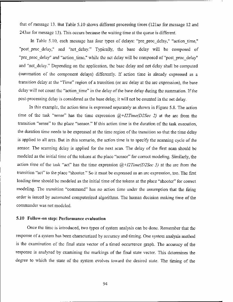
that of message 13. But Table 5.10 shows different processing times (\2lus for message 12 and

243us for message 13). This occurs because the waiting time at the queue is different.

In Table 5.10, each message has four types of delays: "pre_proc_delay," "actionjime,"

"post_proc_delay," and "net_delay." Typically, the base delay will be composed of

"pre_proc_delay" and "actionjime," while the net delay will be composed of "post_proc_delay"

and "net_delay." Depending on the application, the base delay and net delay shall be computed

(summation of the component delays) differently. If action time is already expressed as a

transition delay at the "Time" region of a transition (or arc delay at the arc expression), the base

delay will not count the "actionjime" in the delay of the base delay during the summation. If the

post-processing delay is considered as the base delay, it will not be counted in the net delay.

In this example, the action time is expressed separately as shown in Figure 5.8. The action

time of the task "sense" has the time expression @+I2Time(D2Sec 2) at the arc from the

transition "sense" to the place "sensor." If this action time is the duration of the task execution,

the duration time needs to be expressed at the time region of the transition so that the time delay

is applied to all arcs. But in this scenario, the action time is to specify the scanning cycle of the

sensor. The scanning delay is applied for the next scan. The delay of the first scan should be

modeled as the initial time of the tokens at the place "sensor" for correct modeling. Similarly, the

action time of the task "act" has the time expression @+I2Time(D2Sec 5) at the arc from the

transition "act" to the place "shooter." So it must be expressed as an arc expression, too. The first

loading time should be modeled as the initial time of the tokens at the place "shooter" for correct

modeling. The transition "command" has no action time under the assumption that the firing

order is issued by automated computerized algorithms. The human decision making time of the

commander was not modeled.

5.10 Follow-on step: Performance evaluation

Once the time is introduced, two types of system analysis can be done. Remember that the

response of a system has been characterized by accuracy and timing. One system analysis method

is the examination of the final state vector of a timed occurrence graph. The accuracy of the

response is analyzed by examining the markings of the final state vector. This determines the

degree to which the state of the system evolves toward the desired state. The timing of the

94

response is analyzed by measuring the timestamps of the final state vector, i.e., by examining

how the system meets the timing constraint (or the windows of opportunity).

Figure 5.9 is the timed occurrence graph generated with the maximum information delay.

The reachable state of the system has been reduced from four paths in the untimed occurrence

graph (Figure 5.5) to two paths in the timed occurrence graph (Figure 5.9).

r

|r_u_i. t -vn_ ,Str_\\,£J™

n-------------- |—■ «-_! I. I. llkn

n

■^" ■ h fc ■ «inn

JS Ki.'t L i> r BiBi-n-i

ISK"'' ' ■*"■ ■•»"■■"•■^

122 *-■-,-, ■■

R IM IM—IUr L *^m m. J- b b *■...._ 1^" ■■*- b b *■ npiw^

'■■ »- — ii— b b ^abB^^bt —i __--. ."■i-H-ii. mf

'■■ »—Jb— b b M b iHi|nnr|b i—t.—_*-j«:3(

IJJJJ— b lb_iMlMH I 'nm-.rii b ■ -1 i J~i ■ i ■ ■ ■ i j |nMab._ii__ L. b JU». ■■!—u Ti J.I ■ ■ m ^ ! |fb,JUL bJ.M IUpU^ *

^— — — — — — — — — — — ____ _ _j

!■■■ ■ ii— b hia^uJIrnar?! ■ m ■ , i b b * dn.—i bKiH^JH-fari I rmm ■.■.!!«, b b J^ M^jjlh^i ■*■ ^ .

ir^H ■—j^ b b * ■■■■i iwnva ' !"■■ L_ Jb— b b AH. J- ■Ip^TTl |

Figure 5.9 Full Occurrence Graph from Timed Petri Net

In Figure 5.9, the ordering of the sequence of markings varies depending on the binding of

the initial threats. If the non-hostile threat (i.e., the threat with target ID 2 and with the identity 0)

is processed first by the sensor, the sequence of markings results in M1-M2-M4-M6-M9-M11.

95

Similarly, if the hostile threat (i.e., the threat with ID 1 and with the identity 100) is processed

first, the sequence of markings results in M1-M3-M5-M7-M8-M10.

Tables 5.12 and 5.13 are the state vectors of the final state of the timed occurrence graph

when it was generated with the maximum information delay. If we disregard the timestamps,

both the final state vectors Mil and M10 are identical to the final state vector Mil of the

untimed occurrence graph in Figure 5.5 (note that the timed occurrence graph is a subset of the

untimed occurrence graph.) In the scenario of this example AAW model, the threat was

expressed as tokens at the place "Threat." The final state vector shows no tokens at that place,

i.e., all threats are cleared. The result of the response was expressed as tokens at the place

"Negated." The final state vector shows that the threat with target ID 1 has been "Cleared" (i.e.,

not [ "KillSelf' or "Leak.") So the system responded correctly toward the desired state.

The timestamp of the place "negated" has 0.65 seconds at the state vector M10 and 2.65

seconds at the state vector Mil. The system responded against the threat within the time interval

[0.65, 2.65] seconds. The set of the response time has been derived from all final state vectors

(i.e., all possible sequence of markings; all possible sequence of transitions; all possible sequence

of tasks). Thus this interval of the response time may represent the window of capability of the

system for the worst case since the set of the response times was derived based on the maximum

information delay. However, whether it is a worst case or not depends only on whether the

system responds faster when the information delay is smaller compared to when the information

delay is larger. There is no guarantee when the order of task executions generates different

response times. Comparing this window of capability to the timing constraint, we can verify

whether the system meets the windows of opportunity.

Both the accuracy and the timing of the response for the worst case have been analyzed

using the final state vector and the timed occurrence graph. The same type of analysis can be

done for the minimum and average information delays. Tables 14 through 17 are the final state

vectors for those cases. The time intervals [0.62, 2.62] and [0.63, 2.63] represent the windows of

capability of the system for minimum and average cases, respectively.

96

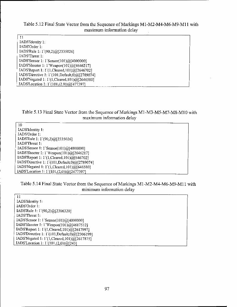
Table 5.12 Final State Vector from the Sequence of Markings M1-M2-M4-M6-M9-M11 with maximum information delay

11 IADS'Identityl: IADS'Orderl: IADS'Rule 1: l'(90,2)@[2335026] IADSThreatl: IADS'Sensor 1: rSensor(101)@[4000000] IADS'Shooter 1: rWeapon(101)@[4646217] IADS'Report 1: l'(l,Cleared,101)@[2646702] IADS'Directive 1: l'(101,Default,0)@[2789074] IADS'Negated 1: r(l,Cleared,101)@[2646580] IADS'Location 1: l'(101,(2,0))@r4773971

Table 5.13 Final State Vector from the Sequence of Markings M1-M3-M5-M7-M8-M10 with maximum information delay

10 IADS'Identityl: IADS'Order 1: IADS'Rule 1: 1\90,2)@[2335026] IADSThreatl: IADS'Sensor 1: rSensor(101)@[4000000] IADS'Shooter 1: rWeapon(101)@[2646217] IADS'Report 1: r(l,Cleared,101)@[646702] IADS'Directive 1: 1\101 Default,0)@[2789074] IADS'Negated 1: r(l,Cleared,101)@[646580] IADS'Location 1: l'(101,(2,0))@[24773971

Table 5.14 Final State Vector from the Sequence of Markings M1-M2-M4-M6-M9-M11 with minimum information delay

11 IADS'Identityl: IADS'Orderl: IADS'Rule 1: l'(90,2)@[2306320] IADSThreatl: IADS'Sensor 1: rSensor(101)@[4000000] IADS'Shooter 1: rWeapon(101)@[4617512] IADS'Report 1: r(l,Cleared,101)@[2617997] IADS'Directive 1: r(101,Default,0)@[2306199] IADS'Negated 1: l\l,Cleared,101)@[2617875] IADS'Location 1: l'(101,(2,0))@r2431

97

Table 5.15 Final State Vector from the Sequence of Markings M1-M3-M5-M7-M8-M10 with minimum information delay

10 IADS'Identity 1: IADS'Orderl: IADS'Rule 1: l'(90,2)@[2306320] IADS'Threat 1: IADS'Sensor 1: l"Sensor(101)@[4000000] IADS'Shooter 1: rWeapon(101)@[2617512] IADS'Report 1: l'(l,Cleared,101)@[617997] IADS'Directive 1: l\101,Default,0)@[2306199] IADS'Negated 1: l'( 1,Cleared, 101)@[617875] IADS'Location 1: l'(101,(2;0))@r20002431

Table 5.16 Final State Vector from the Sequence of Markings M1-M2-M4-M6-M9-M11 with average information delay

11 IADS'Identity 1: IADS'Orderl: IADS'Rule 1: l'(90,2)@[2322028] IADS'Threat 1: IADS'Sensor 1: l'Sensor(101)@[4000000] IADS'Shooter 1: l'Weapon(101)@[4633220] IADS'Report 1: l'(l,Cleared, 101)@[2633705] IADS'Directive 1: l'(101,Default,0)@[2548992] IADS'Negated 1: r(l,Cleared,101)@[2633583] IADS'Location 1: l'(101,(2,0))@[238819]

Table 5.17 Final State Vector from the Sequence of Markings M1-M3-M5-M7-M8-M10 with average information delay

10 IADS'Identity 1: IADS'Order 1: IADS'Rule 1: T(90,2)@[2322028] IADS'Threat 1: IADS'Sensor 1: l'Sensor(101)@[4000000] IADS'Shooter 1: l'Weapon(101)@[2633220] IADS'Report 1: r(l,Cleared,101)@[633705] IADS'Directive 1: l'(101,Default,0)@[2548992] IADS'Negated 1: r(l,Cleared,101)@[633583] IADS'Location 1: l'(101,(2,0))@r22388191

The windows of capability of the system that were derived based on the minimum

information delay may represent the optimistic case (see the lower and upper bounds of the

98

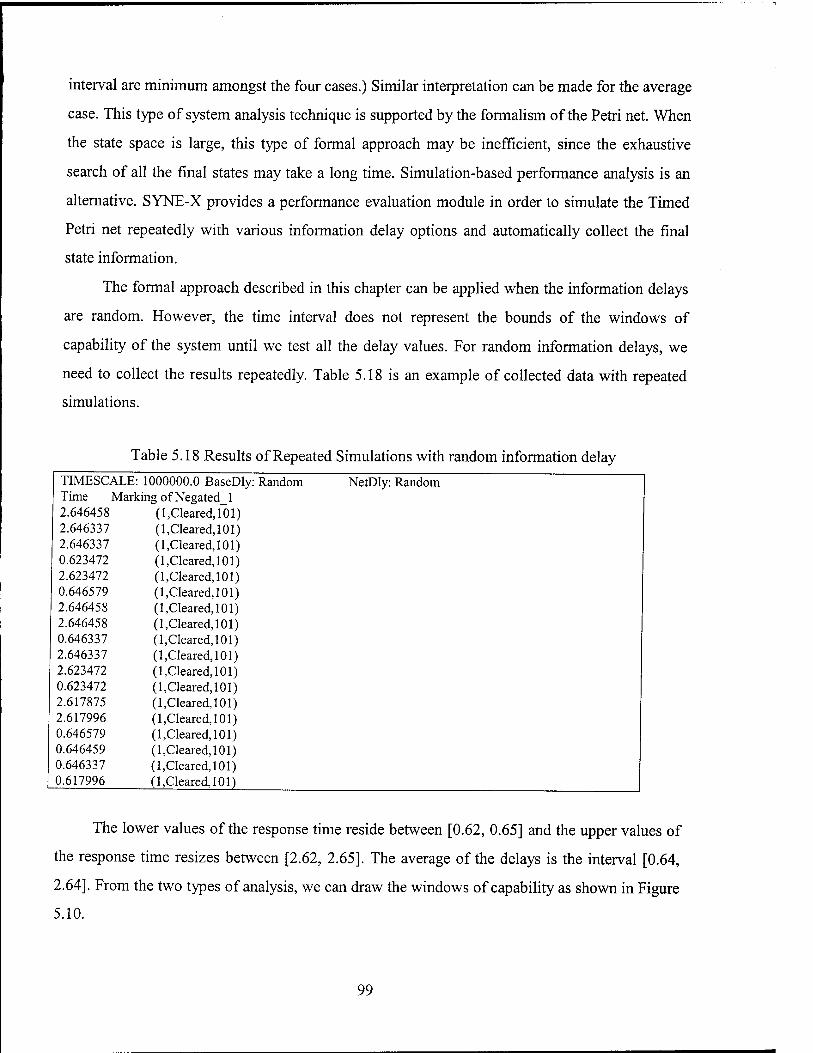
interval are minimum amongst the four cases.) Similar interpretation can be made for the average

case. This type of system analysis technique is supported by the formalism of the Petri net. When

the state space is large, this type of formal approach may be inefficient, since the exhaustive

search of all the final states may take a long time. Simulation-based performance analysis is an

alternative. SYNE-X provides a performance evaluation module in order to simulate the Timed

Petri net repeatedly with various information delay options and automatically collect the final

state information.

The formal approach described in this chapter can be applied when the information delays

are random. However, the time interval does not represent the bounds of the windows of

capability of the system until we test all the delay values. For random information delays, we

need to collect the results repeatedly. Table 5.18 is an example of collected data with repeated

simulations.

Table 5.18 Results of Repeated Simulations with random information delay

TIMESCALE: 1000000.0 BaseDly: Random NetDly: Random Time Marking of Negated 1 2.646458 (1 .Cleared, 101) 2.646337 (1,Cleared, 101) 2.646337 (1,Cleared, 101) 0.623472 (1,Cleared, 101) 2.623472 (1,Cleared, 101) 0.646579 (1,Cleared, 101) 2.646458 (1,Cleared, 101) 2.646458 (1, Cleared, 101) 0.646337 (1,Cleared, 101) 2.646337 (1,Cleared, 101) 2.623472 (1,Cleared, 101) 0.623472 (l,Cleared,101) 2.617875 (1,Cleared, 101) 2.617996 (1,Cleared, 101) 0.646579 (1,Cleared, 101) 0.646459 (1,Cleared, 101) 0.646337 (1,Cleared, 101) 0.617996 (1,Cleared, 101)

The lower values of the response time reside between [0.62, 0.65] and the upper values of

the response time resizes between [2.62, 2.65]. The average of the delays is the interval [0.64,

2.64]. From the two types of analysis, we can draw the windows of capability as shown in Figure

5.10.

99

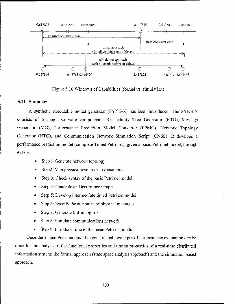
0.617875

^

0.633583

—e— 0.646580

&

2.617875

€+-

2.633583

—e— 2.646580

6 possible optimistic case

-e

possible worst case

-e-

formal approach with all combinations of delays

simulation approach with all combinations of delays

<h -e -e- -e 0.617996 0.63715 0.646579 2.617875 2.63612 2.646458

Figure 5.10 Windows of Capabilities (formal vs. simulation)

5.11 Summary

A synthetic executable model generator (SYNE-X) has been introduced. The SYNE-X

consists of 5 major software components: Reachability Tree Generator (RTG), Message

Generator (MG), Performance Prediction Model Converter (PPMC), Network Topology

Generator (NTG), and Communication Network Simulation Script (CNSS). It develops a

performance prediction model (complete Timed Petri net), given a basic Petri net model, through

9 steps:

Stepl: Generate network topology

Step2: Map physical resources to transitions

Step 3: Check syntax of the basic Petri net model

Step 4: Generate an Occurrence Graph

Step 5: Develop intermediate timed Petri net model

Step 6: Specify the attributes of physical messages

Step 7: Generate traffic log file

Step 8: Simulate communications network

Step 9: Introduce time to the basic Petri net model.

Once the Timed Petri net model in constructed, two types of performance evaluation can be

done for the analysis of the functional properties and timing properties of a real-time distributed

information system: the formal approach (state space analysis approach) and the simulation based

approach.

100

CHAPTER 6. A CASE STUDY

Modern surveillance and tracking systems often use multiple sensors of different types to

provide intelligence to a command organization. Multiple sensors or intelligence agents are

connected through communications networks. The sensors are usually physically dispersed at

geographic locations. What combination of the component systems has the best combat outcome

in terms of the overall force effectiveness? This is a design issue for a system (or resource

allocation) to carry out the mission. Suppose that the data fusion system provides probability

values about the identity and the location of the target continuously. One of the warfightersjfl

problem is how to judge that the object is a hostile threat given the probability values. Decision

makers need to establish a decision threshold.

6.1 Problems in question

The first issue is what is the relationship among uncertainty, decision time, and the effect

of decisions. Altukhov (1984) explained the relationship (Figure 6.1) as follows: there is a certain

level of information for optimal decision when it is assumed that the effect of the decision is

proportional to the level of information available.

When less information is available, it takes a long time to make a decision due to lack of

information. When information is more than sufficient, it takes a long time to process the large

mass of information and results in a delay. He stated that the optimal decision point is to make a

decision when the information level is in the range of c-d in the figure by deriving the required

level of information from the acceptable level of decision effect.

Meanwhile, Van Trees (1989) illustrated the relationship between uncertainty and decision

time using Figure 6.2. Uncertainty decreases over the elapsed time; a decision maker makes a

decision at a certain time accepting a certain level of uncertainty. We can derive two types of

decision constraints to make a decision: time and uncertainty. If the decision time does not affect

the outcome of the decision, then the best decision making point in terms of time is the

maximum time allowed, assuming that the quality of decision is proportional to the information

available. If decision time affects the quality of the decision, there exist some trade-offs between

101

uncertainty and time. From the relations between decision time and uncertainty, we can derive

the operating range (thresholds) of decision making as shown in Figure 6.2.

Optimal Effect

Acceptable Effect

Allowed Time

^. Information

Figure 6.1 Uncertainty, Time, and Decision

timing constraint

acceptable decision threshold

0P(Udec>tdec)=0Ptimal?

min dec max time

Figure 6.2 Operating Range of Decision

If we can measure the performance of the information fusion system in terms of the level of

information at a certain time and the quality of decision made at that time, we can use this

performance measure as an operating factor to make a trade-off between time and uncertainty. If

time and uncertainty have a balanced effect on the outcome of the decision, the command and

102

control process can be defined as a management function of the time-uncertainty factors in

conducting a mission.

Under this definition, we can consider two types of problems in developing a decision

strategy over a command and control timeline. If the problem to be solved has no system noise as

in target identification (it has no system noise because the identity of the target never changes),

then, making a decision at the last moment within the allowed time such as Tmax in Figure 6.2 is

the best decision strategy. The sample graph (Figure 6.3) shows the probability profile of a target

identity over the observation time.

Target Identification

0.8

0.6

-*■ 7*1 T* DTT "^r

-^ ~^-

-O CO

-Q O

ol 0.4

0.2

-i 1 1 i_

2 4 6 8 10 12 14 16 18 20

Observation Time (Sensitivity *: ratio=18, +: ratio=9, o: ratio=6, -: ratio=mixed)

Figure 6.3 Target Identification with Bayesian Rule

The graph was generated by a data fusion system which uses a Bayesian rule with prior

information (probability of hostility 0.5), given that the likelihood ratio (r) of sensor type \ *\-i

103

18 (probability of 0.9 for positive identification and 0.05 for false identification,) the ratio of

sensor type \ +;- is 9 (pr obäüli ty cf 0.9 for peat i \e i datifi at i en and 0.1 for fal se i dertifi at i a\

and the ratio of sensor type ; oj-is 6 (probüli ty of 0.9 fa pcati\e i dertifi at i en andO. 15 fo

false identification) with 2 seconds of the measurement cycle. The dotted line shows the

probability profile obtained by fusing the three sensory data with a centralized data fusion

algorithm with an assumption of conditional independence among the sensor data. The solid line

is the decision threshold (probability of hostility 0.9), required to make a judgment about the

identity of the object. In this system, waiting more time can reduce the uncertainty of the identity.

If a decision maker makes a judgment about the hostility of the object too early, there is a

possibility of wrong judgment. If he waits too long to be confidence of the judgment, however,

there is the possibility of closing the window of opportunity to intercept the object.

If there is system noise as in a target tracking system, waiting more time does not help the

best decision quality once it reaches a certain level. The variance of estimated location can never

be zero-variance when there is system noise even though we measure the track of a target an

infinite number of times. Once the uncertainty reaches the level of the steady-state covariance

(Chang, 1997), it stays constant at the value that corresponds to system noise.

Suppose that a target tracking system measures the location and velocity of target

periodically and estimates the next location with a certain variance. The sample graph (Figure

6.4) shows the change of the variance of the estimated location over the observation time. The

graph was generated by a Kaiman filter with a system of one dimensional constant velocity

model. A target is moving with the velocity 680m/sec and with the initial variance of the

estimated location of 100m. The target has system noise with a Gaussian distribution with zero

mean and the variance of lem/sec. The tracking radar has the measurement noise of a Gaussian

distribution with zero mean and variance of 10 m/sec. The tracking radar scans the target every 2

seconds. In this case, the uncertainty can never be resolved due to the system noise (lem/sec). So

we have to establish an acceptable level of uncertainty such as Umax in Figure 6.2.

104

x 10"3 Target Tracking

9 4-

8 - +

o

LU c o « E CO

LU

7

6

5

4

-

+ +

+ + + + ■ '^ + + -r + -r + + + CD Ü c CO

to >

3

2

1

0 -

-1 ' 2 4 6 8 10 12 14 16 18 20

Observation Time: system noise G(0,0.00001), measurement noise G(0,0.01)

Figure 6.4 Target Tracking with Kaiman Filter

Given a time-uncertainty distribution function of a C3 system, we can derive two types of

operating ranges of decision (Udec and Tdec in Figure 6.2) from those two Tmax and Umax

constraints. Verifying whether the window of capability overlaps with the window of opportunity

is to find the operating range given the time-uncertainty distribution function. Furthermore, after

analyzing the performance of the system behavior within that operating range we can select the

decision-making strategy to optimize the trade-offs between the accuracy and timeliness of the

response.

6.2 Operational concept of an Anti-Air Warfare system

Suppose that there is an air defense system whose mission is to clear air threats when

multiple unknown objects are approaching friendly forces with different velocities at different

locations. If the object is a hostile one, it must be shot down before it arrives at the battle line.

105

This results in a timing constraint on the response. But neutral flights must not be attacked. This

results in an accuracy constraint on the response.

To carry out the mission, an early warning system provides intelligence for the

identification of the objects using a Bayesian rule. A tracking radar provides the estimated

location of the objects using a Kaiman filter. One air defense unit consists of one organic radar

with the capability to track multiple targets with time-sharing protocols, and one missile launcher

with the capability to arm multiple missiles.

An early warning system geographically distributed over the battlefield supports the air

defense unit for identification of targets. Figure 6.5 is the command and control system with two

information fusion systems.

Sense

U1|kby Information Fusion 1 (Bayes Net)

V .—

Command

Detect Threat

j .

(Sensors) u2|k by Information Fusion 2 (Kaiman Filter)

t, Identification

\

Localization

t2 f ion /

Execution

'(u, t) Clear Threat

(Missile)

(Commander)

Figure 6.5 Command and Control of an Anti-Air Warfare System

The variables of interest are:

• Uijk: Uncertainty of target identity at time k,

• ti : Decision Time to use Ui

• U2|k : Uncertainty of target location at time k,

• t2: Decision Time to use U2

• C(u?t): command order under uncertainty U at time t

The identity of the object is either hostile (H) or neutral (Hc). The target identification

system observes the features of targets recursively and calculates the probability of the identity

pi|(e, k)' and decides the identity 1^ t]^ with a decision thresholds (acceptable probability and

106

allowed time,) where Ui is the uncertainty at the decision time ti. Figure 6.6 represents this

Bayesian fusion engine.

The motion of a target is specified by both location (L) and velocity (V). The target

tracking system observes the movements of targets recursively and estimates the variance of

estimation Swl , and decides whether to re-localize or not with decision thresholds (acceptable M|(e, k) v r

variance and allowed time,) where u2 is the uncertainty at the decision time t2. Figure 6.7

represents this information fusion engine that uses a Kaiman Filter for a one dimensional

constant velocity model.

Decision Threshold 1: dth p t maxI

Threat ID: !->{H, Hc

Bayes Net rI|(e,k)

i Identification

I(uU1) -> {H*, ff*} ►

Sensor_Tja2£_3VCOMINT)

Sensor Tjmeij^ELINT)

Sensor Type l)( MINT)

Figure 6.6 Data Fusion for Target Identification

Decision Threshold 2: dth2, t

Threat Motion : ^Mj(e,k) M -> (L, V}

w Kaiman Filter

T M(u2,t2) ->(L*.V) Localization ^

i \

J(4/16T)

Scan Cyc]e_2_Jii2/16 T) )(1/16T)

Figure 6.7 Data Fusion for Target Tracking

107

Finally, the fire direction commander issues a command order C/u (y whether to fire (F) or

not (F ) using the information from the data fusion systems as shown in Figure 6.8. The fire

decision is governed by the decision threshold. An engagement rule forces the weapon system to

not fire a missile against a neutral object.

(Engagement Rule)

L ■ C(u,t)->{F,P} Command

I(ul,a) -> {H-, H<*}

M(u2,2, "> (L*. V*) X

Figure 6.8 Command Decision

Suppose that the number of missiles per target is limited due to the resource constraints. To

carry out the mission successfully, we need to address the following questions:

• What kinds of design choices do we have?

• How do we develop decision thresholds?

• What do we do to resolve the tolerance of the network delays?

6.3 Experimental system design

From the mission statement in the previous section, the global inputs and outputs of the

experimental system have been identified as shown in Figure 6.9.

The scenario is follows. The threats are characterized by their identity (e.g., hostile flight,

friendly force flight, decoy, a flock of birds, etc.), their initial location, their velocity, and their

number. Each threat has a different probability of detection according to the avenue of approach,

such that the probability is low in mountainous areas and high in open areas. The interceptor of

the AAW system is characterized by the location of its initial deployment, its velocity, firing

range, and probability of kill. The AAW system should handle multiple threats. But there is a

limited number of resources. The weapon platform (missile launcher) can load multiple missiles

at the same time and it takes a certain time to reload after firing one.

108

Threat

(Information Collection Strategy)

i (dth„tmaxl)

I(u,tI) ->{H*,H<*}

(dth2'tmax2)

M, (u2,t2) -> (L*, V*)

(Engagement Rule)

c(u,t)->{F,p; RD(U,0 ->{ KillH, ► KillHc,

Miss H Miss Hc ■ Leak }

Figure 6.9 The Anti-Air Warfare System of the example

The output of the combat operations is assessed as one of three combat results; jfikll ene rry

(H)ifJjfMll notrd c)jfJ andjfjleatyfl. Tie results jfMl ljfl or jfl eal$ flare affected by the respo nse t

the system and jfilill iß er jfMl c are affected by the uncertainty level at the decision time. The

result jfiklljflor jfinhssjfl depend on the prchtility cfkill of the interceptor. It is a ssirsd,

simplicity, that the probability of kill is determined by the accuracy of the estimated location of

the target. If the variance of the accuracy is within the hit range of the interceptor, the target is

killed. Once the result is identified as a jfi rhssjf] the interceptor fires repeatedly \üle the target i

within the windows of opportunity.

The sensor is characterized by its type (i.e., identification and tracking), the likelihood ratio

of identification (i.e., likelihood ratio of positive identification over false identification), the

variance of estimated location and velocity, the surveillance range, scan cycles, and the number

of sensors. Multiple sensors are configured for centralized data fusion.

Figure 6.10 is the deployment diagram of all the resources of the AAW system attached to

the communication network, in which

• X_n: a node of the communication network. The bandwidth of a link between nodes is

1,024 Mbps; the electronic propagation delay of each link is 10ms.

109

• Sn: a surveillance radar that performs mainly identification of targets within the area of

interest (i.e., global battle area); calculates locally the probability of target identification

using Bayesian updates; and reports the probability of identity and trajectory data to

centralized data fusion center (AWACS).

• Rnnn: a tracking radar that performs only the tracking of targets within the area of

responsibility (i.e., local area assigned to the battery); and reports the trajectory data to

the local fire direction center (FDQ.

• Wnnn: a weapon that intercepts targets and launches missiles following the order from

the local FDC.

{FDC {Display} 10Mb 10ms LL Queue/DropTail Mac Channel Phy/WirelessPhy}

{AOC {Screen} 10Mb 10ms LL Queue/DropTail Mac Channel Phy/WiredPhy}

Figure 6.10 Deployment Diagram of an AAW system

FDC. a computing device of the fire direction center of the local battery. It calculates

the target trajectory using tracking data from its local tracking radar (Rnnn) and global

110

surveillance radar (Sn); displays the trajectory on the terminal (Display). FDC and

Display are connected to a wireless local area network whose bandwidth is 10Mbps;

the electronic propagation delay of the LAN links is 10ms.

• AOC: a computing device of the global Air Operations Center. It receives target

information (identification and tracking data) from AWACS; allocates targets to each

local battery (FDC); issues a firing order under centralized air control doctrine;

maintains the status of the battlefield and displays the tactical picture on the terminal

(Screen). AOC and Screen are connected to a wired local area network whose

bandwidth is 10Mbps; the electronic propagation delay of the LAN links is 10ms.

• AWACS: a computing device of the early warning system. It calculates target identity

using data from multiple sources and uses a centralized data fusion algorithm.

It is assumed and illustrated by the dotted square box in Figure 6.10 that the computing

devices of all resources connected to the network have the data processing rate of 100 Mbs by

which all incoming and outgoing data are processed bit by bit sequentially.

The problem is to choose a design option to resolve the tolerance of the network delays that

may affect the result of combat, and to develop the decision threshold. The system will be used

under different tactical operational environments. To represent the situation, two rules of

interception have been established:

• Aggressive Intercept: when the object is identified as a threat (i.e., a hostile target), the

system should intercept it regardless of the current location of the target before the object

arrives at the battle line.

• Defensive Intercept: when the object is identified as a threat (i.e., a hostile target), the

system should intercept it when the target is within a specified firing zone (e.g., within

the arbitrary interval [10km, 40km] from the battle line; see Figure 2.1).

An executable performance prediction model has been designed with seven input

parameters, in addition to the rules of interception, and four output performance measures. The

parameter variables are:

• Number of Sensors: one of three {#1, #2, #3} surveillance radars plus 1 tracking radar;

each additional sensor has the next longer surveillance range from the set {short, medium,

long}; for the experiment, ranges of {40km, 70km, 150km) were used (these are arbitrary

111

numbers: 40km has been chosen from the line-of-sight range on the sea surface, the

others from the typical criterion to classify short and long range radar).

Number of Transponders: One transponder(s) per sensor from the set {single, multi). It

may be a design alternative for a multi-purpose radar since multi-transponders have the

effect of reducing the scanning cycle and increasing the number of sensors. The scanning

cycle may have critical impact to track multi-threats in a time sharing surveillance mode.

In the experiment, eight transponders were used. Given that the scanning cycle of a sensor

is 2 seconds (rotate 30 times per minute), the eight transponders will reduce the scanning

cycle to 2/8 seconds assumed that all eight transponders are equally spaced.

Sensor Likelihood Ratio: The probability of positive identification over the probability of

false identification. It takes one of the values from the set {6, 9, 18}.

Computation Rule for Fusion: The computation for data fusion is dynamic ox fixed.

When some sensor data is unavailable due to any reason (by the sensor being out-of-

service, by jamming of communication link, by non-detection of the target, or by the

different surveillance ranges of sensors in operation, etc.), the computation for data fusion

needs to have a rule or to wait until the remaining sensor data arrive; if more than one

sensor is in operation and if the sensor data is received from only a partial number of

sensors at a specific time, the jfidyna rhqfl c onpiteti on rule uses the partial sensor cat

only for fusion (a set of conditional probability matrices was used for this rule);

meanwhile the ;ffi xedjfl c orrputEt i en rule keeps each sensor cata at the store and uses th

stored data together with the partial information received.

Surveillance Mode: Either of active or passive surveillance mode. If the uncertainty of a

target does not meet the decision criterion, the jfiacti vejfl rule assign? pried ty to the use cf

specific sensor for the specific target until the uncertainty decreases so that a judgment

can be made; the passive' rule scans the battlefield in routine manner without priority;

when the target is a High Valued Target (HVT), the HVT will have priority so that the

target is intensively searched and tracked. In the passive mode, the sensor scans the

battlefield periodically every two seconds in the case of a sensor with a single transponder

and every 2/8 seconds of a sensor with eight transponders. In the active mode, the sensor

allocates all time slots to the specified target.

112

• Information Delay: It includes information processing time and the information

distribution delay. It takes one of the values from the set {zero, min, max, random}.

• Decision Threshold: The decision criterion for making a judgment whether the object is a

hostile target or not. If the probability of the target identity is larger than the threshold, the

target is considered as a hostile target and a fire order is issued. It takes one of the values

from the set {0.7, 0.8, 0.9,0.99}.

The effectiveness of the system was measured by:

• Mission Success: the ratio of the number of threats cleared over the total number of

threats within the allowed time. It measures performance in a [0.0,1.0] scale.

• Decision Quality: the ratio of the number of correct decisions over the total number of

decisions. It measures performance in a [0.0,1.0] scale.

• Weapon Efficiency: the ratio of the number of threats cleared over the number of

interceptors (i.e., missiles) used. It measures performance in a [0.0, 1.0] scale.

• Operational Readiness: the time at which the system finishes all the tasks and switches

the operation mode into the idle state. It measures performance in unit s of time.

The information delay and the speed of the interceptor may significantly affect the

timeliness of the system. Similarly, the probability of kill may significantly affect the weapon

efficiency of the system. In this experiment, the variance of track estimation was used to

determine the probability of kill (see Appendix C for details). The speed of the interceptors was

set at Mach 3 for every interceptor.

6.4 Synthetic executable model of the AAW system

To measure the performance of the AAW system, a performance prediction model has been

developed. Figure 6.11 is the top-level diagram of the AAW system. It is an extension of Figure

5.2.

The model shows four values (0.7, 0.8, 0.9, and 0.99) for the decision threshold to be used

as a criterion for making a judgment about the hostility of the objects (the initial marking of the

place named rules of engagement). It also shows four threats with seven attributes (the initial

marking of the place named threat): target nomination (threat ID), identity (PH), velocity (V),

113

initial location (Lo), initial variance of track parameter (S0), probability of detection (PD), and the

event occurrence time of the threat.

SurveilIance_Directive

/•""Directive rule_s

rule_s

Threat threat Sense tacpicture

|H II

1'(1 ,(R2I 1 0),2,30,(R2I 0.1 ),(R2I 0.9),(D2Sec 0))++ l'(2.(R2I 1.0),2,50.(R2I0.1),(R2I 0.9),(D2Sec 0))++ l'(3,(R2I 1.0),2.70,(R2I0.1),(R2I 0.9),(D2SecO))++ l'(4.(R2I 1.0),2.90,(R2I0.1).(R2I 0.9),(D2Sec 0))

tacpicture

1 '[(R2I 0.7),(R210.8),(R2I 0.9),(R2I 0.99)]

Rules_of_Engagement

"RUHT

tacpicture TacticalPicture Negated

Figure 6.1 lTop Level Diagram of an AAW system

The arbitrary characteristics of the threats that were used in this experiment are shown in

Table 6.1. The life time of the threats (timing constraints or windows of opportunity) varies

depending on the rule to intercept the threats: aggressive intercept or defensive intercept since a

rule specifies the firing zone (see also section 2.2 in Chapter 2). Table 6.2 shows the timing

constraints that the AAW system must meet as derived from the rules of interception and the

arbitrary characteristics of the threats. For example, the threat with ID 4 must be intercepted in

the time interval [0.0, 132.35] seconds under the aggressive intercept rule and [73.53, 117.65]

seconds under the defensive intercept rule.

114

Table 6.1 Arbitrary Characteristics of Threats

Threat ID PH V Lo So PD to 1 1.0 Mach 2 30km 100m 0.9 0.0 2 1.0 Mach 2 50km 100m 0.9 0.0 3 1.0 Mach 2 70km 100m 0.9 0.0 4 1.0 Mach 2 90km 100m 0.9 0.0

Table 6.2 Timing constraints of the AAW system (in seconds)

Target ID Aggressive Intercept Defensive Intercept 1 [0.0, 44.12] [0.0, 29.41] 2 [0.0, 73.53] [14.705, 58.82] 3 [0.0, 102.94] [44.117, 88.24] 4 [0.0, 132.35] [73.529, 117.65]

Suppose that a sensor periodically scans the battlefield and provides the FDC with sensory

data about the identity and the location of the object as shown in Figure 6.4. If we choose the

decision threshold 0.9, it takes 9 seconds with high and medium sensitivity (likelihood ratio 18

and 9) and 11 seconds with the low likelihood ratio (likelihood ratio 6) for the sensor to provide

the required information. If we disregard the information delay, all threats except the threat with

ID 1 under the defensive intercept rule can be cleared. Suppose the sensor has a single built-in

transponder, tracks the object in the time-sharing protocol, and processes the ID 1 threat after the

other three threats. Then it needs a minimum of 27 seconds to process the other three threats and

only 2.41 seconds to process the threat ID 1. Clearly, one sensor with a single transponder cannot

guarantee the success of the mission when all four threats are incoming at the same time. At

least, we need to increase either the number of sensors with single transponder or the number of

transponders of a single sensor. Then, how many sensors or transponders are needed to guarantee

the successful completeness of the mission? To answer this type of question, multiple sensors

were used to measure the MOEs. Figure 6.12 shows the centralized configuration of three

sensors (see Figure 2.5).

115

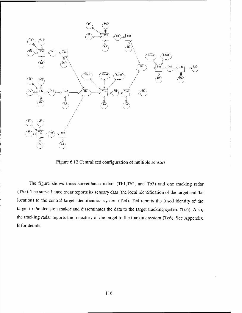
,/TT^ ,/MI\

^ Tc6 j_>j4(6Y_cj Td6 i ,JO$

Figure 6.12 Centralized configuration of multiple sensors

The figure shows three surveillance radars (Tbl,Tb2, and Tb3) and one tracking radar

(Tb5). The surveillance radar reports its sensory data (the local identification of the target and the

location) to the central target identification system (Tc4). Tc4 reports the fused identity of the

target to the decision maker and disseminates the data to the target tracking system (Tc6). Also,

the tracking radar reports the trajectory of the target to the tracking system (Tc6). See Appendix

B for details.

116

The threats trigger information flow between tasks and in turn generate the traffic in the

communications network. How does the information delay affect the success of the mission? To

estimate the node processing delays and network transmission delays, an executable physical

model has been developed. Figure 6.13 is the executable physical model implemented using

Network Simulator (1999).

0—€>

Figure 6.13 Executable Physical Model

The nodes with the circle symbol in Figure 6.13 represent the communication network

nodes and those with the hexagon symbol represent the information processing nodes. A

processing node estimates the data processing time of incoming and outgoing data. The delay

time includes the residual time of a message waiting in queue while the computing device is in

service for other messages. The directed bars on each link represent the message flow over the

links for emulation.

The delay values have been estimated using the TCP protocol for the messages of

command information (e.g., fire order) and the UDP protocol for the common tactical picture

(e.g., sensory data messages). The network may be commonly used for other C4ISR systems. To

117

represent this, the simulation has also been run with background traffic: a traffic bias level

between all network nodes with the UDP protocol, a message inter-arrival time of two seconds,

and the lowest priority versus the highest priority messages of the AAW system.

During the simulation, the size of all message has been arbitrarily set to 1000 bytes The

size of message to be processed for data fusion at each sensor may be different according to the

characteristics of the sensor. For example, if a sensor performs image processing, the size may

depend on the resolution of image taken by the sensor. These messages sizes have also been

arbitrarily set to 100 Kbytes for all types of sensors.

6.5 Findings

The results of the experiment are shown in Appendix C.

• Number of Sensors and/or Transponders: In general, more sensors or more transponders

produce higher effectiveness. However, the relation was not true in the case of ihefixed

computation rule.

• Computation Rule: The dynamic computation for data fusion supports better timeliness

(operational readiness) than the fixed computation rule, even though the decision criterion

of the dynamic computation rule has a higher threshold than that of the fixed computation

rule.

• Number of Sensors vs. Computation Rule: In the dynamic computation for data fusion, as

the number of sensors increases, the system shows better timeliness (operational

readiness). However, the opposite was true in the fixed computation rule.

• Decision Threshold: Clearly, there is a relationship between the decision criterion and the

success of mission. If we focused on the timeliness of a response, the lower threshold for

the decision criterion is preferred. However, if we focused on the accuracy of a response,

the higher threshold is preferred.

• Decision Threshold vs. Computation Rule: In the dynamic computation rule for data

fusion, the decision threshold needed to be set to the higher value for better performance.

This is reasonable because this computation rule loses the benefit of multiple sensors

since it uses a partial number of sensors, and so the higher threshold is required to get

higher quality of information. Conversely, in the fixed computation rule for data fusion,

118

the decision threshold needed to be set to the lower value. This rule fuses data assuming

there are multiple sets of sensory data. It takes a long time to reach the higher threshold

when some sensory data is unavailable. So, it is reasonable that the lower threshold is

required to respond quickly.

• Information Delay: Obviously the information delay should affect the timeliness of the

response. But it was not true that the minimum information delay always guarantees the

fastest response. It means that the information delay affects the behavior of the system not

just in terms of the timeliness, but also the ordering of tasks in an autonomous system

depending on the arrival time of information. It is conjectured that, once the information

processing and distribution systems have the potential capability to carry out the mission

successfully, the performance of the system (response time) may be more highly affected

by the order of the information arrivals than by the delay of information.

Throughout the results, when a system consisting of a data fusion sub-system with a single

transponder was used, the possible combinations of input parameters to meet the performance

requirements were restricted. When multiple transponders were used, there were many more

possible combinations of input parameters that met the performance requirements.

Based on this experiment, the, fixed computation rule shows better weapon efficiency than

the dynamic computation rule does. It can be interpreted that the estimation of the tracking

system with the fixed computation rule provides a more accurate target trajectory. This is

reasonable for this experiment, since the dynamic computation rule uses the partial set of local

sensory data at the time of computation disregarding the old information stored at the central data

fusion system, while the fixed rule uses the full sensory data stored at the central data fusion

system. For more realistic analysis, the tracking algorithm may need to be implemented in more

detail.

6.6 Answers to War-Fighterjft Qiesti on

In general, the number of transponders per sensor has a critical impact: the more

transponders the better. Given the number of transponders, if there are multiple sensors and if

the data fusion system is used in an autonomous firing mode by the computerized automated

system,

119

• under an unstable system operational environment due to any reasons (poor survivability

of sensors, jamming on the communications link, etc.),

• if the ranges of surveillance radars are different, or

• if the probability of target detection is low

then, the data fusion system must be designed using the dynamic computation rule for data

fusion and the decision criterion for the judgment of threat identification needs to be established

with the higher threshold. More sensors will increase system performance.

If the data fusion system is designed using the fixed computation rule, as the number of

sensors increases, there is possibility that the system effectiveness may decrease. So the number

of sensors needs to be chosen properly. More experiments are required using parameters under

the stable system operational environment, identical surveillance ranges, and higher probability

of target detection. In the scenario of this experiment, the lower decision criterion threshold

increased performance. The decision threshold needs to be reexamined if the fixed computation

rule is used under different scenarios.

120

CHAPTER 7. CONCLUSIONS

7.1 Summary

Many of the C3 systems in the real world are supported by a common network or a network

of networks. Predicting the performance of a C3 system consisting of sub-systems requires the

integration of such sub-system models with the communication system models. When the system

is used for a time critical mission, the network delay may play a decisive role in battle

management. So, the integrated model must be able to represent the network delay properly.

Ensuring that the system responds within the windows of opportunity (i.e., meeting the timing

constraints) requires estimation of the bounded values of the task connection delays over the

network.

In the model of synthetic execution, the architecture of a system has been represented in

two layers: the functional architecture layer and the physical architecture layer. The physical

architecture consists of the communications model and the resources (sensors, computing

devices, weapon systems, etc.) that are attached to the network. The approach presented in this

thesis models both architecture layers as executable models. Then both layered executable

models are combined for performance prediction. Total ordering of events is the core of the

theoretical background of the approach. State space analysis techniques are used for the total

ordering of events and a discrete event simulation technique is used for execution, preserving the

total order.

The executable functional model uses a Petri net to describe the logical behavior and the

executable physical model uses a queueing net to represent the demand and the contention of

resources necessary to implement the logical behavior. The message-passing pattern is generated

from the reachability tree of the executable functional model. The executable physical model

processes those messages preserving the message-passing pattern.

Once the network delay is measured in the executable physical model, the delay value is

inserted into the executable functional model. The resulting Timed Petri net

121

model allows both formal state space analysis and simulation for performance prediction of a

real-time distributed system. By examining the timestamps of all the possible final states of the

system, the windows of capability can be measured so that they can be used to verify whether the

system responses are within the windows of opportunity. By examining the markings of all the

possible final states of the system, the accuracy of the response can be measured. When the

system is a large-scale system and suffers from state space explosion, the simulation technique

can be used for efficient analysis.

7.2 Advantages and limitations of the approach

The major advantages of the synthetic execution approach for performance prediction of a

real-time distributed system are as follows. In synthetic execution, the time values are estimated

by a separate communication network model rather than directly modeling the contention of

communication resources as a single integrated model. The communication service demands are

isolated from the functional model. This enables the executable functional model to be invariant

with respect to the executable physical model. Because of the invariant feature of the functional

model from the physical model:

• Efficient collaborative work between teams is possible in designing the functional

and physical architectures, and

• Existing communication models can be easily reused.

This may provide higher efficiency in developing large-scale system models through the

development cycle from the early stage of system design to performance prediction. Because the

Petri net formalism is used as the basis of the synthetic execution model for performance

prediction:

• The strengths of both formal and simulation-based approaches for performance

evaluation can be obtained;

• The synchronization problem, one of the major issues in military doctrine, is

resolved by the model's net structure.

The use of the discrete event simulation technique rather than the probabilistic queueing

model as the executable physical model, allows the following:

• Communications models can be specified in any preferred level of detail, and

122

• Realistic representation of communications is possible, since the messages are

captured from the state space of the functional model and processed in total order in

the physical model.

The limitation of the approach arises from the state space explosion problem of the

occurrence graph of the Petri net. The method for capturing the total order from the occurrence

graph of the Petri net model will be used efficiently for a conflict free net since one path of the

occurrence graph contains all the required information needed for total ordering of events. A

non-conflict free net may have multiple final states. Even if the net has a single final state,

different paths can have different orderings of events resulting in different total orders. For

theoretical soundness, the approach requires the repetition of the procedures from the first step to

the last step as many times as the number of different total orders. Given the two assumptions

about the characteristics of the communications network: (1) network delays are longer under

heavier traffic loads than under lighter traffic loads, and (2) the degree of traffic load is defined

as the amount (e.g., number or size) of messages in a given time interval, the total order of events

based on the longest path from the initial state to final state may be used for efficiency. The

approach needs to generate the full occurrence graph to find the longest path when the net is not

conflict free. Unless we can model the system with the conflict free net structure1, the approach

presented in this thesis does not address the inefficiency problem.

7.3 Future Research Directions

In conclusion, the major contributions of this dissertation are as follows.

• A model of synthetic execution of a real-time distributed system has been

developed so that both logical and timing behavior of system can be predicted.

• A method for capturing ä realistic traffic pattern based on the logical behavior of a

system has been developed.

An "off-line" simulation technique using the synthetic execution model has been presented

to avoid the inefficiency of the "run-time" distributed simulation protocol when the distributed

models have different time scales. When the executable physical model is large, it may be

1 The author believes that most information system models for C4ISR systems can be modeled with the conflict free net structure.

123

partitioned into several parts for engineering level efficiency in simulation. In this case, one may

want to use the "run-time" distributed simulation technique on the engineering level. A

comparison of "off-line" and "run-time" simulation techniques can be conducted.

Suppose that multiple heterogeneous systems use different network resources, but share

some resources. The order of message passing between tasks from different functional

architectures of the multiple heterogeneous systems may have the precedence relations of events

depending on the interactions amongst the multiple systems. Suppose that there is a mission to be

carried out by two systems: a combat service support system (CSS) and a force maneuvering

control system (MCS). The message passing between tasks to carry out the mission represents

the logistics flow and the force movement over the transportation network with limited terrain

resources in addition to the information flows over the communication network for command

and control. Across the boundaries of the multiple systems, some sets of messages may have

multiple time lines. Currently the methodology has been developed for performance prediction of

information systems. Also the simulation of the executable physical model (i.e., the queueing net

model transformed from the Petri net model) schedules the events in total order over the single

time line. The theoretical challenge for future research is to expand the synthesis method to deal

with multiple functional architectures with non-monotonic time. The notion of vector and matrix

time that are extensions of the scalar time introduced in Chapter 3 may offer insight to this

extension. It is believed, however, that the methodology presented in this dissertation could be

used by scaling up the boundary of the system. By aggregating component systems, we can scale

up the boundary of the system. Then the total order of events can be captured from the scaled-up

system. Finally the two heterogeneous physical network models can be executed while

preserving the total order. The "run-time" distributed simulation of the two separate physical

network models may be suitable for implementation.

124

125

APPENDIX A. COMPUTER IMPLEMENTATION OF COLORED PETRI NETS:

DESIGN/CPN

A.l Colored Petri Nets

While ordinary timed or untimed Petri nets offer a mathematical way of modeling

complex concurrent and asynchronous processes, their usefulness is limited, in part,

because the tokens are indistinguishable. Modeling even a simple system can result in

very complex structures using ordinary Petri nets. Colored Petri nets are a full extension

of ordinary Petri nets that provide a very compact way of modeling complex systems.

Colored Petri nets use the same structure as ordinary Petri nets. They consist of places,

arcs, transitions, and markings. In addition, in Colored Petri nets, tokens are no longer

indistinguishable. They can take on attributes or values, sometimes referred to as colors.

The values or colors for tokens are defined using color sets. A color set is a vector of

attributes. These attributes can be any standard data type, integers, reals, characters,

strings, enumerated, etc. Any particular token is characterized by the values assigned to

each of the attributes in the vector that defines its color set. The term color was derived

by an analogy to the color wheel, in which any color in the visible spectrum can be

defined by the strength of each of the three colors (attributes), Red, Green, and Blue. By

introducing these color sets, it is possible to reduce the complexity of the structure of an

ordinary Petri net model, although rules governing the enablement and firing of

transitions become more complex.

126

Design/CPN is a graphical computer tool that supports the construction, simulation,

and logical, behavioral, and performance evaluation of CP net models. Thus it has three

components, a graphical editor for construction, a simulator for both graphical and

automatic simulation, and a State Space analyzer for evaluation. A CP net is constructed

as a drawing. It consists of places, shown as ellipses, transitions, drawn as rectangles, and

arcs connecting places to transitions and transitions to places. By convention, places and

transitions are given names written inside the places or transitions. The names have no

formal meaning but they can have a significant impact on the readability of the net.

Design/CPN allows the use of variables to represent, in a compact way, different

enabling conditions of transitions. A token is an element of a given color set and can only

take the values defined by the color set. The definition of the color sets and of the

variables is done in the Global Declaration Node. Color sets in Design/CPN correspond

to types in a programming language such as Pascal or C and can be of two types: atomic

and complex. An atomic color set is a color set whose elements are of a simple type.

Examples of atomic color sets are: enumerated, integer, real, string, etc. A complex color

set is a color set obtained by combining different color sets. Examples of complex color

sets are product, union, list, records, etc. Variables can be defined for the color sets to be

used in the model.

A place can only contain tokens of a given color set. The color associated with a

place is written in italics and must be declared in the Global Declaration Node. The

marking of a place is defined as a multiset and is written:

127

M(pO = ^iiih'ah. h = l

where riih is the number of tokens of color ajh in place pi. The initial marking of a

place, which is the number and type of tokens contained in the place at the beginning of

the simulation, is underlined. For example the marking of a place P containing two blue

tokens and three red tokens is written:

M(P) = 2'blue + 3'red

Annotations on the arcs specify the number and the color of tokens that the arcs can

carry and are written in the form of multisets. The number and the color of tokens can be

specified as variables. Variables defined for color sets are handled like an element of this

color set.

An arc expression can contain if-then-else or case statements to represent different

possible combinations of tokens that can be carried on the arc. A transition is enabled

when the tokens in the input places satisfy the arc expression connecting those places to

the transition. When the transition fires, it removes from the input places as many tokens

of the colors defined in the input arc expression and generates in the output places as

many tokens of a color as specified by the arc expressions connecting the transition to the

output places. Enablement of a transition results in the binding of color set variables to

tokens contained in the input places. This binding of variables remains the same for the

generation of tokens. An example is shown on Figure A.l.

128

pi l"big+r small

color Sample = with blue | yellow | red; var s : Sample; color Size = with big | small;

if(s=red)then l'big else rsmall

tl p3

O if(s=red)thenrblue ^/g

else Tred+ryellow

Sample

Figure A.l Example of Variable Binding

Two color sets have been defined in the Global Declaration Node: Sample is an

enumerated color set and contains the elements blue, yellow and red; Size is also an

enumerated color set and contains the elements big and small. A variable s has been

defined for the color set Sample. Place PI has the color set Size associated with it and

contains as initial marking 1 big token and 1 small token. Places P2 and P3 have the color

set Sample associated with them. Place P2 contains initially one red token. The use of the

variable s on the arc expression allows to represent different combination of tokens for

the enablement of transition tl. The variable s is first bound to a color contained in place

P2. According to the value taken by the variable s, one big token or one small token

contained in place P2 is used for the enabling of the transition. If the required token is not

present in place PI, the transition is not enabled. When the transition fires, the enabling

tokens are removed from places PI and P2 and the tokens specified by the output arc

129

expression are generated in place P3: if s is bound to red then one blue token is produced,

otherwise one red and one yellow tokens are produced in place P3. For the initial marking

specified for places PI and P2, the variable s is bound to red and the transition tl is

enabled because the required big token is present in place PI. When the transition tl fires,

the big token is removed from place PI and the red token is removed from P2; one blue

token is generated in place P3.

One can see from this example that the use of variables and if-then-else statements

is a practical implementation of the matrices associated with the arcs in the formal

Colored Petri Nets. The main advantage is that the use of variables and if-then-else

statements can be used for large color sets while matrices on large color sets are hardly

usable.

To facilitate the specification of different enablement of a transition, Design/CPN

allows the use of a guard function associated with the transition. A guard function is a

Boolean expression operating on the variables used in the input arc expression. A

transition is thus enabled if the input places contain the tokens specified by the input arc

expression and if the guard function associated with the transition evaluates to true.

Finally, in Design/CPN, the firing of a transition can trigger the execution of a code

segment associated with the transition. A code segment is a piece of code written in ML

(Meta Language) which is a functional programming language and that can be used either

to generate the attributes of the tokens put in the output places or to perform any

operations not directly related to the simulation of the Colored Petri Net such as storing

130

of data in a file or automatic updating of a chart. Figure A.2 displays a simple Colored

Petri Net which uses guard functions and code segments.

Global Declaration

Color Set*- Order

Arc Expression -*- V order

r threat

Threat

color Order = with wait | fire; color Threat = with hostile | neutral; color Response = with Monitor | Engage; var order : Order; var threat: Threat; var response: Response;

[threat = hostile] -*-Guard Function

V response (y Response

input (threat,order); output (response); action if order = fire then Engage else Monitor

Figure A.2 Example of a Colored Petri Net in Design/CPN

The Global Declaration Node defines three color sets: Order contains the elements

wait and fire, Threat contains the elements hostile and neutral, and Response contains the

elements Monitor and Engage. A variable for each of these color sets is defined. A color

set associated with each place defines the type of tokens that each place can contain. Each

arc is assigned an expression that specifies the number and type of tokens that needs to go

through the arc. For example 1 'threat means that one token of color set Threat can go

through the arc. The expression threat=hostile (or "threat equal to hostile") is the guard

function of the transition. The guard function adds another condition that must be

131

fulfilled besides the presence of tokens in the input places. Finally, the code segment

specifies how the output token is generated from the input token. For example, if a threat

is hostile and the order is fire then the response is Engage; otherwise Monitor the threat.

A.2 Timed Colored Petri Nets

Time is introduced into Colored Petri Nets as follows. The tokens that are sensitive

to time must belong to a color set defined as timed in the Global Declaration Node. Each

token belonging to a timed color set has a timestamp associated with it represented by the

suffix of the type @[n] where n is the simulation time at which the token will be

available: if n is less than the simulation time, the token can not enable any transition. If n

is equal or larger than the simulation time, then the token is available. The timestamp of a

token is updated in two ways: through the firing of a timed transition or a timed arc

expression. A timed transition is a transition having a time region which contains an

expression of the type @ -{-(expression) where expression can be a finite value, a variable,

or a function of variables returning an integer or a real value which will be the delay

associated with the transition computed for the values of the variables. When a timed

transition fires, timed tokens are put in the output places as defined by the output arc

expressions with a timestamp equal to the current simulation time augmented by the

value of the expression of the time region. If a transition has no time region, the

timestamp associated with the timed tokens put in the output places is equal to the current

simulation time. One can see that this is a variation of the transition model of time in

132

Ordinary Petri Nets. The only difference is that reserved tokens are generated in the

output place instead of having enabling tokens become reserved in the input places. A

timed output arc expression is an expression associated with an output arc of the type

n'(expression 1)@^(expression 2) where expression 1 defines the tokens that need to be

put in the output place, and expression 2 defines the timestamp that needs to be

associated with the tokens. A timed arc expression can only be used for arcs that connect

a transition to a place whose color set has been defined as timed in the Global Declaration

Node. When a transition fires, timed tokens are put in the output places as defined by the

output arc expressions with a timestamp equal to the current simulation time augmented

by the value of the time expression of the arc expression. One can see that the use of

timed arc expression corresponds to the implementation of the place model of time in

Ordinary Petri Nets.

The use of the variation of the transition model and of the place model provides

flexibility in the use of time in CP nets. Sometimes it is more natural to associate a time

delay with a process that is modeled by a transition, and other times a time delay

associated with an arc that represents the transfer of the output of a process to another

process is more appropriate. Both models can be used at the same time in a model. When

a timed arc expression is used with a timed transition, the time expression of the arc

expression is added to the transition timed region so that the output token has a

timestamp equal to the current model time augmented by the sum of the two time regions.

Figure A.3 illustrates the handling of time in Colored Petri Nets. The transition

process models a process that needs to be triggered and that takes for inputs il and

133

produces, after a processing time of 10 units of time, an output ol. Output ol is retained

locally and so there is no transmission delay to send it to other process. After the

initiation of a process a report rpt has to be sent and there is a delay of 2 time units for the

transmission to other process. The status of the process is turned to on just after initiation.

Trigger rtriE@ri51 (fT

l'il@f51

color Trigger = with tr ig timed; color Input = with i 1 | 2 timed; color Output = withol | o2 timed; color Report = with rpt timed; color Status = wirh on off;

Report

Output

Trigger Report

Yxp\@+y© IIEM271 Output

rol+(@) rol@[251

Status

simulation time: 5 simulation time: 15

Figure A.3 Firing of a Timed Transition

In the Global Declaration Node, the color sets Input, Output, Report and Trigger

are declared as timed. During execution, the Design/CPN starts with the model time equal

to zero. There are no enabled transitions at this model time. The simulator advances the

model time to the earliest time that will enable any transition. In the left hand side of the

figure, the transition is enabled only when the simulation time reaches 15 at which the

token 1 'trg at the place Trigger is available. The marking of the net obtained after firing

of the transition at time 15 is shown on the right hand side. The token 1 "rpt in the place of

134

color set Report has a timestamp equal to 27 as the result of the time expression @+10 at

the time region of the transition plus the timed arc expression 1 'rpt@+2, while the token

ol has a timestamp equal to 25 because of the time expression @+10 at the time region

of the transition. Finally, the token Von in the place of color set Status does not have a

timestamp because this color set has not been declared as timed and therefore the token

on is immediately available to enable other transitions.

A.3 Hierarchical Colored Petri Nets

The modeling of a large-scale system leads to a Colored Petri Net representation

which is very large and that cannot be easily looked at and analyzed. The notion of

Hierarchical Colored Petri nets has been introduced in Design/CPN to deal with this

problem. A set of transition and its interconnecting places can be replaced by a

substitution transition, which then refers to a subpage containing the subnet which

replaces this substitution transition. This substitution process preserves the logical

consistency and the dynamical behavior of the system model. In Figure A.4, the subnet

made of transition t2, t3 and t4 and their interconnecting places p4, p5, p6 has been

replaced by the substitution transition st, this subnet being displayed on another page

referred to as the Hierarchical Substitution (HS) region of the substitution transition.

Places p2, p3 and p7 that represent the interface between the subnet and the remaining of

the net are duplicated on the subpage. These places are called socket nodes in the upper

page and port nodes in the lower level page. There is a one to one correspondence

135

between a socket node and a port node: they are virtually the same place and the marking

of a socket node is the same as the marking of the port node.

An interesting feature of Hierarchical Colored Petri Nets is that different

substitution transitions can refer to the same subnet. To each of these substitution

transitions corresponds a different instance of the subnet that behaves independently of

the other instances. The distinction between the different instances is made through the

correspondence of socket nodes at the upper level and port nodes of the instance at the

lower level. The development of Colored Petri Net model can then be done through the

development of independent and reusable modules arranged in a hierarchical structure

that looks like a lattice. Any change in a subpage will affect all its instances but will not

affect the rest of the model as long as the correspondence between the socket nodes of the

upper level page and the port nodes in the lower level page is maintained.

136

lower page P2 p5

IH'nQ-

0" @

P3

P7

t4

t3

o ff] Out

Figure A.4 Substitution Process

137

APPENDIX B. DESCRIPTION OF THE PETRI NET MODEL OF THE AAW

SYSTEM

High level representation of sensor operation

Surveillance_Directive

l'(l,Default,0)++ l'(2,Default,0)++ l'(3,Default,0)++ l'(5,Default,0)

P In

Threat

SensorsA Surveillance Directive

Operate Sensors

Identity^ r^r^

TacticalPicture

TacticalPicture

Figure B.l Petri Net Diagram: Sense

The diagram in Figure B.l is the substituted transition of sense in the top-level

diagram (Figure 6.11). AWACS receives the surveillance directive from AOC. An

intelligence collection unit operates their organic sensors and disseminates the

intelligence (identity and location of targets) to the combat units in the battlefield

138

(identification to AOC and location to FDQ. By default, it collects data using the active

scanning mode. In the active mode, it scans and tracks the specified target only with

higher priority to collect more intensive data for the target. In the passive mode, it scans

and tracks the targets periodically without the priority.

By changing the marking of the place Sensors, it represents the number of sensors

in operation. The transition Operate Sensors is decomposed into the lower level in the

hierarchy. The label AWACS in the dotted box is the name of the physical node (see

Figure 6.10) assigned to carry out the logical task (i.e., transition Update Directive). The

label [0,0] means the action time to carry out the task.

Decomposition of sensor operation

The diagram in Figure B.2 is the substituted transition of Operate Sensors in Figure

B.l. The nodes Sense 1, Sense2, and Sense3 are the substitution transitions of surveillance

radar 57, S2, and S3 in the physical architecture (Figure 6.10), respectively. The node

Sense5 is the substitution transition of the tracking radar R101 in the physical

architecture. The nodes Sense4 and Senseö are the substitution transitions of central data

fusion nodes AWACS and FDC in the physical architecture, respectively. The label

EXTERNAL in the dotted box is the name of the physical node assigned to carry out the

logical task (i.e., transition Generate). Since this transition is an event generator for

simulation, no physical resource is assigned.

139

Surveillance_Directive

Piiln i

[o.oi ;

[EXTERNAL]"

'lnggef\

Threat

->, Generate I Threat

/FOA

FacT

Fact

\J*

Sense5

m

Sense3

LH]

Sense 1

rai

Sense2

m

Sense4

m

Sense6

^

_/1>ensörsN ,—„ ,

J;

ES

TacticalPicture

ES —©

TacticalPicture

Figure B.2 Petri Net Diagram: Operate Sensors

140

Operation of a local sensor

l'[(l.(0.(R2I0.5),l,l,(R2IO.O),(R2I0.1),(D2SecO)),0)]

SurveilIance_Directive

(^\ Store

8?

Parameters

l'[(l.(D2Sec 2).(map R2I [0.15.0.9.0.002.150.0])),(l,(D2Sec 2),(map R2I [0.1,0.9,0.001,150.0])),(l,(D2Sec 2),(map R2I [0.05,0.9.0.001,150.0]))]

Figure B.3 Petri Net Diagram: Sense 1

The diagram in Figure B.3 is the substituted transition of Sensel in Figure B.2. The

local sensor (Tbl) detects targets, calculates and maintains (at the place store) the

probability of target identity and the variance of tracking data, and sends (by Tdl) the new

target information to central data fusion node. The identification algorithm has been

implemented using Bayesian rule to update the new probability. The tracking algorithm

has not been implemented using a full Kaiman filter. For simplication, only the variance

of track estimation was computed. The purpose of tracking data in the scenario is to

141

determine the probability of kill such that, if the variance of the estimated location of the

target is less than a certain criteria, the result is jfiMlljflotherwse jfbnssj fl. This scena

requires the variance only. Thus the algorithm has been simplified and computes only the

variance of the estimation.

The label R101 in the dotted box is the name of the physical node (see Figure 6.10)

assigned to carry out the logical task (i.e., transitions Tbl and Tdl). The label [0,2] and

[0,0] mean the action times to carry out the tasks. The interval [0,2] means that the

transition Tbl scans the battlefield periodically every 2 seconds. The time 0 represents the

time that the target can be detected at any time of the cycle. It can be used to estimate the

maximum processing time and the maximum network delay under assumptions about the

characteristics of information system and communications network. The interval [0,0]

means that the transition Tdl has no action time because it only disseminates the target

information, and so it has only the network delay.

The parameter of the sensor is represented by the marking of the place Rl. From the

left in the data structure of the marking (l,(D2Sec 2),(map R2I ([0.05,0.9,40.0]))), 1

represents the sensor ID, (D2Sec 2) represents the default action time (the default scan

cycle of 2 seconds), and [0.05,0.9,40.0] represents [probability of false detection,

probability of positive detection, surveillance range] in which that the sensitivity

(likelihood ratio) is 18 and the surveillance range of the radar is 40.0 km.

142

Target identification; Sense 6 has the same structure

Store /SUOTN, I'[(1,(0,(R2I0.5),1,1,(R2I0.0),(R2I 1.0),(D2SecO)),0)]

Store ^W4^, l'[(2,(0,(R2I0.5),l,l,(R2t0.0).(R211.0),(D2SecO)),0)l

Store f S3to4 1 r[(3,(0,(R2I0.5),l,l,(R2I0.0),(R2I1.0),(D2Sec0)),O)]

04 r04 FG V

Distributed

Distributed

Rules Store

l'|(4,(D2Sec 0).0.(map R2I [0.0,1.0])),(4,(D2Sec 0).0,(map R2I [0.0,0.5,0.5,1.01)),(4,(D2Sec 0),0,(map R2I [0.0,0.25.0.25,0.75,0.25,0.75,0.75,1.0]))]

Figure B.4 Petri Net Diagram: Sense4

The diagram in Figure B.4 is the substituted transition of Sense4 in Figure B.2. This

fusion node (Tc4) calculates and maintains the probability of target identity and the

variance of tracking data from three sensors, and disseminates (by Td4) the new target

information.

143

The label AWACS in the dotted box is the name of the physical node (see Figure

6.10) assigned to carry out the logical task (i.e., transitions Tc4 and Td4). The label [0,0]

means the action time to carry out the task.

The fusion rule is represented by the marking of the place R4. From the left in the

data structure of the marking (4,(D2Sec 0),0,(map R2I ([0.0,0.5,0.5,1.0]))), 4 represents

fusion node ID, (D2Sec 0) represents no action time, 0 is the counter to be used for FIFO

(First In First Out) processing of incoming sensory data, and [0.0,0.5,0.5,1.0] represents

the conditional probabilities of the target identity for data fusion dealing with two sensory

reports in order of [FF,FT,TF,TT] in which FF means the conditional probability when

two sensors reports that the target is a non-hostile object and TT means the conditional

probability when two sensors report the target is a hostile object.

Command Function

The diagram in Figure B.5 is the substituted transition diagram of command in the

top-level diagram (Figure 6.11). The transition Decide make a judgment whether the

target is hostile or not using the probability of target identity and issues the firing order if

the probability meets the decision criteria (threshold). The results of the combat received

from each platform is displayed on Screen and maintained in a database (place Cleared).

If the target is assessed to be jfi rhssjfl, it issues the firing orcfer again to any a^älä)!

interceptor. The decision is made by the automated computing algorithm. If the

uncertainty (i.e., probability) does not meet the decision criteria, the algorithm issues the

144

new surveillance directive in order to switch the surveillance mode from default mode

(Passive mode) to Active mode (i.e., scan or track only the specific target).

P In

■ P In

^Identity"

TacticalPicture

Rules_of_Engagement

"Rule

[0,0]

r[ÄÖC]

Decide

/'"'Reporf'

Report

. [0,0]

[Screen] ▼ /

Assess

IPJ | I/O I

ProcessedThreat ( ) I'D

Order

SurveilIance_Directive

Figure B.5 Petri Net Diagram: Command

The label AOC in the dotted box is the name of the physical node (see Figure 6.10)

assigned to carry out the logical task (i.e., transitions Decide). The label [0,0] represents

the action time to carry out the task. It does not have the human decision making time due

145

to the automated algorithm. The label Screen is the physical device to display the tactical

picture after the actions taken.

Act function

Order

Order

TacticalPicture

;[0,0] ;

1 [Display]

updateTask

[0,0] ;

■ [Display]

updateTrack M—

i'[]

bracks

Contact

OrderList

Tasks l'[]

Intercept

/'^VeaponN

Assets

4'(0,3,0) Report

Figure B.6 Petri Net Diagram: Act

This diagram in Figure B.6 is the substituted transition of act in the top-level

diagram (Figure 6.11). The transition update task receives an air tasking order from AOC,

update the current mission on Display of FDC, and sends the order to the platform

(transition node Intercept). The transition update track receives the target track

146

information for localization and update the current location on Display of FDC, and

sends the track to the platform (transition node Intercept).. The platform (transition

Intercept) checks (the marking at the place named Weapon) the availability of a missile

and launches it when available. The initial marking shows that the platform has 4 missiles

armed. After elapsing the flight time that are required to intercept the threat, the platform

reports the after action report (AAR).

The label SIOI in the dotted box is the name of the physical node (see Figure 6.10)

assigned to carry out the logical task (i.e., transition Intercept). The label [0,5] and [0,0]

mean the action times to carry out the tasks. The interval [0,5] means that the platform

(transition Intercept) needs 5 seconds to reload the missile after firing one. The time 0

represents the time that the target can be detected at any time of the cycle. It can be used

to estimate the maximum processing time and the maximum network delay under

assumptions about the characteristics of information system and communications

network. The interval [0,0] means that two transitions update task and update track has

no action time other than information processing to update and display. The label Display

is the physical device to display the current mission and the current location of the target.

The availability of missiles are represented by the markings of the place weapon.

The data structure of the marking represents (weapon ED, velocity, location). For

example, 4'(1,3,0) represents a platform (ED 1) has 4 missiles with velocity Mach 3 and

the initial deployment location 0.

147

APPENDIX C. PERFORMANCE MEASURES FOR THE AAW SYSTEM

C.l Experimental Results

The titles of tables from Table C.l through Table C.22 represent a set of input

parameters that are listed in order of rule of intercept, criteria to assess combat result,

number of transponders, surveillance mode, and information delay. For simplicity, the

variance of track estimation was used to determine the probability of kill so that the

probability can be used to assess the combat result. In this experiment, for simplification,

the probability of kill was used either 1.0 or 0.0 (it was assumed if the variance of the

track estimation is less than a criteria, the probability of kill equals 1.0, otherwise 0.0).

The criteria were represented by the parameter j SXXJ- in t betitle of each table, j SO

represents that the criteria was disregarded: the probability of kill is always 1.0 once the

missile is launched and meets the timing constraint. ; S10;- represents tht the criteria va

1.0 m: if the variance is lees than 1.0 m, the probability of kill is always 1.0, otherwise

0.0.

For example, the \ ^g-esive_S00_Single_Active_Dynamics_Zero;- cf Table Cl,

represents that the simulation has been conducted with the / °aggress vj±rüe cf i rtercep,

the probability of kill 1.0 (j°S00j±/ ^n^i±transponde) / adiv\± surveillance node,

/ ° fynam\±co npilsti onfcrfusion, and/ Zerodnformation delay.

The left 4 columns of each table are also the input parameters used in the

experiment. As the column titles represent, they are snumber of sensor\ + Likelihood

148

Ratio\+ decision threshold]* and information delay\± Te parameter value of

^information delay\± nay have 4 vd ues i n so rro taHex 1 f cr rhri numdday 2 f cr

random delay, 3 for maximum delay, and 4 for zero delay.

The right 4 columns are the performance measures (MOPs). The analysis has been

conducted with the requirements of MOPs: mission success = 1.0, decision quality = 1.0,

and weapon efficiency = 1.0. So the data set only shows a subset of the results that meets

the requirements. The results of the MOPs in every row represent the average of 50 runs

and the value was represented as an index of MOEs.

Table C.l MOEs: Aggressive_SOO_Single_Active_Dynamics_Zero

No of Sensor

Likelihood Ratio

Decision Threshold

Information Delay

Mission Success

Decision Quality

Weapon Efficiency

Operational Readiness

3 18 0.99 4 1 1 1 29.066 3 9 0.9 4 1 1 1 30.333 3 6 0.99 4 1 1 1 41.866

Table C.2 MOEs: Aggressive_S00_Single_Active_Fixed_Zero

No of Sensor

Likelihood Ratio

Decision Threshold

Information Delay

Mission Success

Decision Quality

Weapon Efficiency

Operational Readiness

3 6 0.7 4 39.333 3 18 0.7 4 39.866 3 9 0.7 4 41.666 3 6 0.8 4 44.533 3 18 0.9 4 79.266

Table C.3 MOEs: Defensive_S00_Single _Active_Dynamic_Zero

No of Sensor

Likelihood Ratio

Decision Threshold

Information Delay

Mission Success

Decision Quality

Weapon Efficiency

Operational Readiness

149

Table C.4 MOEs: Defensive_SOO_Single_Active_Fixed_Zero

No of Sensor

Likelihood Ratio

Decision Threshold

Information Delay

Mission Success

Decision Quality

Weapon Efficiency

Operational Readiness

3 18 0.7 4 1 1 1 79

Table C.5 MOEs: Defensive_SOO_Multi_Active_Dynamics_Random

No of Sensor

Likelihood Ratio

Decision Threshold

Information Delay

Mission Success

Decision Quality

Weapon Efficiency

Operational Readiness

1 18 0.99 2 1 1 1 78.729 1 9 0.9 2 1 1 1 78.748

Table C.6 MOEs: Defensive_SOO_Multi_Active_Fixed Random

No of Sensor

Likelihood Ratio

Decision Threshold

Information Delay

Mission Success

Decision Quality

Weapon Efficiency

Operational Readiness

1 18 0.99 2 1 1 1 78.737 1 6 0.99 2 1 1 1 78.739 1 9 0.99 2 1 1 1 78.744

Table C.7 MOEs: Aggressive_SOO_Single_Active_Dynamics_Random

No of Sensor

Likelihood Ratio

Decision Threshold

Information Delay

Mission Success

Decision Quality

Weapon Efficiency

Operational Readiness

3 18 0.99 2 1 1 1 28.859 2 6 0.99 2 1 1 1 38.993 3 6 0.99 2 1 1 1 39.214

Table C.8 MOEs: Aggressive_S00_Single_Active_Fixed_Random

No of Sensor

Likelihood Ratio

Decision Threshold

Information Delay

Mission Success

Decision Quality

Weapon Efficiency

Operational Readiness

2 6 0.8 2 1 1 1 43.828 3 9 0.8 2 1 1 1 44.293 3 6 0.7 2 1 1 1 45.192 3 6 0.9 2 1 1 1 81.374

150

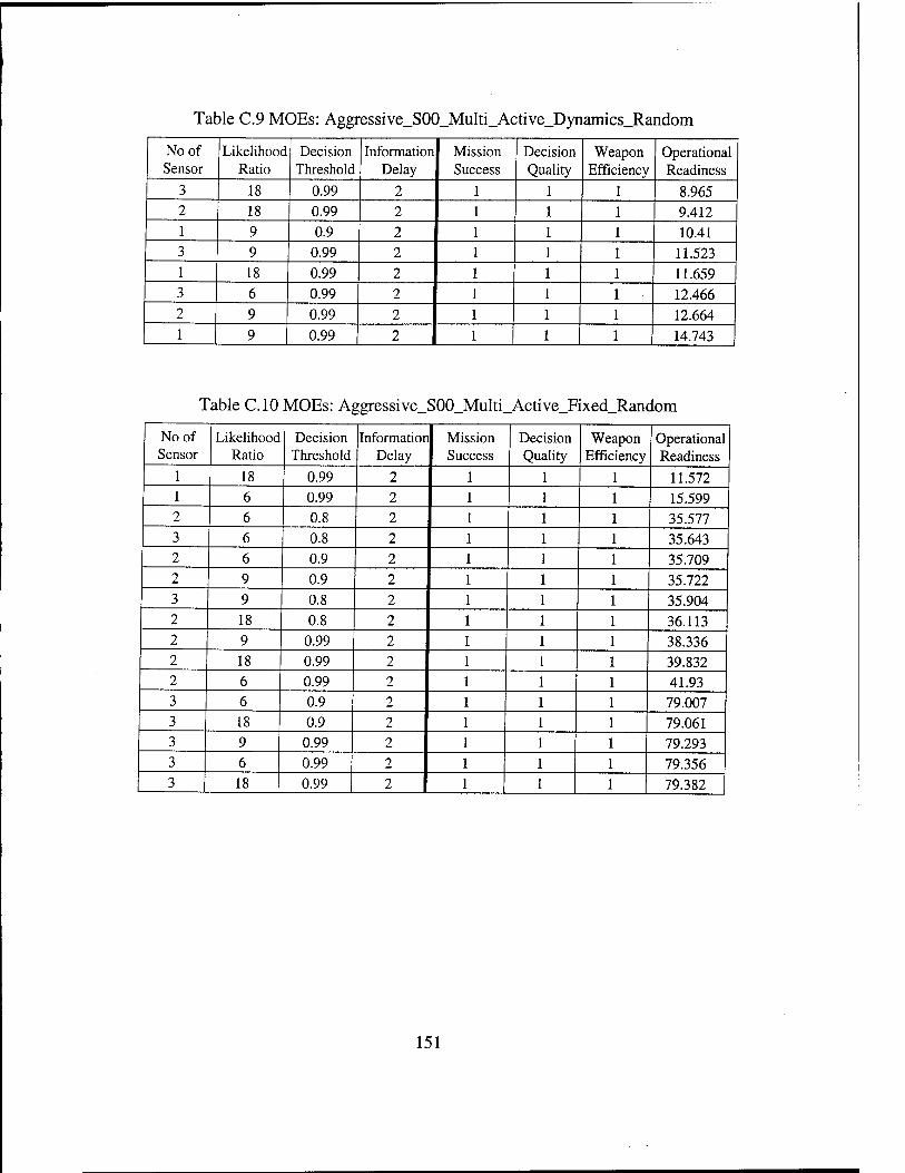
Table C.9 MOEs: Aggressive_SOO_Multi_Active_Dynamics_Random

No of Sensor

Likelihood Ratio

Decision Threshold

Information Delay

Mission Success

Decision Quality

Weapon Efficiency

Operational Readiness

3 18 0.99 2 8.965 2 18 0.99 2 9.412 1 9 0.9 2 10.41 3 9 0.99 2 11.523 1 18 0.99 2 11.659 3 6 0.99 2 12.466 2 9 0.99 2 12.664 1 9 0.99 2 14.743

Table CIO MOEs: Aggressive_ S00_Multi_ _Active_Fixed_Random

No of Sensor

Likelihood Ratio

Decision Threshold

Informatior Delay

Mission Success

Decision Quality

Weapon Efficiency

Operational Readiness

1 18 0.99 2 11.572 1 6 0.99 2 15.599 2 6 0.8 2 35.577 3 6 0.8 2 35.643 2 6 0.9 2 35.709 2 9 0.9 2 35.722 3 9 0.8 2 35.904 2 18 0.8 2 36.113 2 9 0.99 2 38.336 2 18 0.99 2 39.832 2 6 0.99 2 41.93 3 6 0.9 2 79.007 3 18 0.9 2 79.061 3 9 0.99 2 79.293 3 6 0.99 2 79.356 3 18 0.99 2 1 1 79.382

151

Table C.l 1 MOEs: Defensive_SOO_Single_Active_Dynamic_Zero with a requirement (mission success = 1.0)

No of Sensor

Sensor Sensitivity

Decision Threshold

Information Delay

Mission Success

Decision Quality

Weapon Efficiency

Operational Readiness

3 6 0.9 4 1 0.988 79 3 9 0.7 4 1 0.955 79 3 18 0.8 4 1 0.946 79.066 3 6 0.7 4 1 0.944 79 3 6 0.8 4 1 0.944 79 3 18 0.9 4 1 0.944 79 2 18 0.9 4 1 0.927 79 3 9 0.8 4 1 0.911 79

Table C.12 MOEs: Defensive_S00_Single_Active_Dynamic_Zero with a requirement (decision quality = 1.0)

No of Sensor

Sensor Sensitivity

Decision Threshold

Information Delay

Mission Success

Decision Quality

Weapon Efficiency

Operational Readiness

3 18 0.99 4 0.983 1 0.983 79 1 18 0.99 4 0.95 1 0.975 79.066 2 18 0.99 4 0.925 1 0.95 79 3 9 0.99 4 0.908 1 0.933 79 2 9 0.99 4 0.883 1 0.95 79 2 6 0.99 4 0.833 1 0.916 79 1 6 0.99 4 0.808 1 0.93 79

Table C.13 MOEs: Defensive_S00_Single_Active_Fixed_Zero

No of Sensor

Likelihood Ratio

Decision Threshold

Information Delav

Mission Success

Decision Quality

Weapon Efficiency

Operational Readiness

3 18 0.7 4 1 1 1 79 2 18 0.7 4 1 0.988 1 79 2 2 1 1

18 18 18 18

0.8 0.99 0.7

0.99

4 4 4 4

0.916 0.775

1 0.9

1 1

0.926 1

0.95 0.938

1 0.958

79 79

79.066 79.133

152

Table C.14 MOEs: Aggressive_S00_Single_Active_Dynamics_1024

No of Sensor

Likelihood Ratio

Decision Threshold

Information Delay

Mission Success

Decision Quality

Weapon Efficiency

Operational Readiness

3 6 0.99 1 1 39.193 3 6 0.99 2 1 39.214 3

3 6 6

0.99

0.99 3 4

1

1 39.739 41.866

3 18 0.99 1 1 32.125 3 18 0.99 2 1 28.859 3 18 0.99 3 1 26.495

3 18 0.99 4 1 1 1 29.066

Table C.15 MOEs: Aggressive_S10_Single_Active_Dynamics_Random

No of Sensor

Likelihood Ratio

Decision Threshold

Information Delay

Mission Success

Decision Quality

Weapon Efficiency

Operational Readiness

2 18 0.99 2 1 1 1 29.22 2 9 0.99 2 1 1 1 38.215 1 18 0.99 2 1 1 1 38.369 3 9 0.99 2 1 1 1 38.548

Table C.16 MOEs: Aggressive_S10_Single_Active_Fixed_Random

No of Sensor

Likelihood Ratio

Decision Threshold

Information Delay

Mission Success

Decision Quality

Weapon Efficiency

Operational Readiness

2 9 0.8 2 1 1 41.799 2 9 0.9 2 1 1 43.561 2 18 0.9 2 1 1 44.027 3 9 0.8 2 1 1 44.173 3 6 0.8 2 1 1 45.336

Table C.17 MOEs: Aggressive_S10_Multi_Active_Dynamics_Random

No of Sensor

Likelihood Ratio

Decision Threshold

Information Delay

Mission Success

Decision Quality

Weapon Efficiency

Operational Readiness

3 18 0.99 2 1 1 9.704 1 9 0.9 2 1 1 10.938 2 9 0.99 2 1 1 11.683 3 9 0.99 2 1 1 12.151 1 6 0.99 2 1 1 16.528

153

Table C.18 MOEs: A ggressive_S 10_Multi _Active_Fixed_Random

No of Sensor

Likelihooc Ratio

Decision Threshold

Information Delay

Mission Success

Decision Quality

Weapon Efficiency

Operational Readiness

1 9 0.9 2 11.283 1 9 0.99 2 14.39 2 6 0.9 2 35.738 3 6 0.8 2 35.842 2 18 0.8 2 35.847 3 9 0.7 2 35.858 3 18 0.7 2 35.863 3 9 0.8 2 35.913 2 9 0.9 2 36.239 3 18 0.8 2 36.577 2 18 0.9 2 36.713 2 18 0.99 2 38.659 2 9 0.99 2 39.313 2 6 0.99 2 41.581 3 9 0.9 2 78.961 3 6 0.9 2 78.97 3 18 0.9 2 78.978 3 18 0.99 2 79.25 3 6 0.99 2 79.322 3 9 0.99 2 1 79.37

Table C.19 MOEs: Defensive_S10 _Single_Active_Dynamic_Random

No of Sensor

Likelihood Ratio

Decision Threshold

Information Delay

Mission Success

Decision Quality

Weapon Efficiency

Operational Readiness

3 18 0.99 2 1 1 0.973 80.958

Table C.20 MOEs: Defensive_S10_Single_Active_Fixed_Random

No of Sensor

Likelihood Ratio

Decision Threshold

Information Delay

Mission Success

Decision Quality

Weapon Efficiency

Operational Readiness

3 9 0.7 2 1 1 1 80.132

154

Table C.21 MOEs: Defensive_S10_Multi_Active_Dynamics_Random

No of Sensor

Likelihood Ratio

Decision Threshold

Information Delay

Mission Success

Decision Quality

Weapon Efficiency

Operational Readiness

2 9 0.99 2 0.993 79.558 3 9 0.99 2 0.986 80.308 3 18 0.99 2 0.98 78.714 2 9 0.9 2 0.973 82.021 1 18 0.99 2 0.966 80.402

2 18 0.99 2 1 0.966 82.84

Table C.22 MOEs: Defensive S10 Multi Active Fixed Random

No of Sensor

Likelihooc Ratio

Decision Threshold

Information Delay

Mission Success

Decision Quality

Weapon Efficiency

Operational Readiness

3 18 0.8 2 78.716 3 6 0.8 2 78.717 3 18 0.7 2 78.719 2 6 0.99 2 78.721 2 18 0.9 2 78.722 2 18 0.99 2 78.726 1 18 0.8 2 78.727 2. 18 0.8 2 78.729 1 6 0.9 2 78.733 2 6 0.9 2 78.733 1 18 0.99 2 78.735 2 6 0.7 2 78.737 3 6 0.7 2 78.737 2 9 0.99 2 78.74 3 9 0.8 2 78.74 2 9 0.9 2 78.745 2 6 0.8 2 78.751 3 9 0.9 2 78.915 3 18 0.9 2 78.964 3 6 0.9 2 79.021 3 18 0.99 2 79.321 3 9 0.99 2 79.349 3 6 0.99 2 1 1 79.46

155

C.2 Observations of system behavior

Before examining the result of the experiment, let us see the general characteristics

of a sensor system. The characteristics of a sensor system are associated with the number

of observations. To analyze the general characteristics of the system behavior, it may be

reasonable and preferable to focus on the tactical operation environment with the

aggressive intercept rule. The defensive intercept case does not respond, even if the

uncertainty requirements are met, until the target moves into a specified zone.

If we make a decision at the last moment, it may reduce the operational readiness

(the time to be ready for the next mission) resulting in the next threat leaking and so fail

to carry out the mission successfully. If we make a decision early, it may reduce the

quality of the decision resulting in killing friendly forces. This type of dilemma may

occur in a time critical decision environment. So it may be reasonable and preferable to

focus on the tactical operation environment with the defensive intercept rule since it has

the smaller windows of opportunity.

The probability of kill and the information delay can be ignored for analysis of the

pure sensor system j ft perf cr nance

Number of Sensors and/or Transponders

In general, more sensors or more transponders produce higher effectiveness.

In a tactical situation of aggressive interception, the system with only three sensors

meets the requirements of mission success and decision quality, if the sensor has a single

156

transponder (see Table C.l and Table C.2). When the window of opportunity is smaller

(i.e., the system is operated under defensive intercept rule; see also Table 6.2), the system

with even three sensors was not enough to meet the requirements if the sensors have a

single transponder and if the dynamic computation rule for data fusion is applied (see

Table C.3). In the fixed computation rule case, the system with three sensors with the high

likelihood ratio meets the requirements (see Table C.4).

With the system with multi transponders, however, the system with even one sensor

meets the requirements (see Table C.5 and Table C.6)

Computation Rule vs. Timeliness

The dynamic computation for data fusion supports better timeliness (operational

readiness) than the fixed computation rule, even though the decision criterion of the

dynamic computation rule has a higher threshold than that of the fixed computation rule.

In the defensive interception rule, the system does not respond, even if the decision

is made, until the target moves into a specified zone. So the situation with the defensive

intercept rule is not good sample space for the general analysis of the relationship

between timeliness and computation rule. The analysis of this general relationship has

been conducted with the situation with the aggressive interception rule.

Compare the operational readiness of Table C.l and the one of Table C.2. For

example, the operational readiness of the system of three sensors with the likelihood ratio

18 is 28.86 in the dynamic computation rule and 39.87 in the fixed computation rule. The

dynamic computation for data fusion supports better timeliness (operational readiness)

157

than the fixed computation rule, even though the decision criterion of the dynamic

computation rule is higher than that of the fixed computation rule. The same relationship

has been observed in Table C.7 and Table C.8. For example, the operational readiness of

the system with the likelihood ratio 6 is 38.99 for two sensors and 39.21 for three sensors

in the dynamic computation rule. The corresponding ones in the fixed computation rule

are 43.83 seconds and 81.37 seconds.

This relationship is clearly shown from the sensor system with multi-transponders.

Compare the operational readiness of Table C.9 and Table CIO in which the results were

sorted by the operational readiness. Consider the system of three sensors with the

likelihood ratio 18 at which the identical decision criterion 0.99 was used. In the dynamic

computation rule, the operational readiness shows 8.97 seconds (minimum value)

meanwhile the one in the fixed computation rule 79.38 seconds (maximum).

Number of Sensors vs. Computation Rule

In the dynamic computation for data fusion, as the number of sensors increases, the

system shows better timeliness (operational readiness). However, the opposite was true in

the fixed computation rule.

See the operational readiness of Table C.9 and the one of Table CIO. Consider the

system of three sensors with the likelihood ratio 18 at which the identical decision

criterion 0.99. In the dynamic computation rule case, the operational readiness of the

system marks 11.66, 9.41, and 8.97 for one, two, and three sensors respectively. In the

fixed computation, however, the corresponding operational readiness shows 11.57, 39.83

158

and 79.83. The same relationship exists in the system of the likelihood ratio 9 and 6. The

operational readiness of the system with the likelihood ratio 9 in the dynamic

computation shows in the decreasing order such as 14.74, 12.66, and 11.52 as the number

of sensors increases. Meanwhile, the operational readiness of the system with the

likelihood ratio 6 in the fixed computation marks in the increasing order such as marks

15.60,41.94, and 79.36 as the number of sensors increases.

Decision Threshold

Clearly, there is a relationship between the decision criterion and the success of

mission. If we focused on the timeliness of a response, the lower threshold for the

decision criterion is preferred (see Table C.ll whose data set shows only those results

meeting the requirement of mission success=l). However, if we focused on the accuracy

of a response, the higher threshold is preferred (see Table C.12 whose data set shows only

those results meeting the requirement of decision quality-1).

Table C.ll and Table C.12 are good examples since the system does not meet both

requirements (mission success=l and decision quality-V) at the same, and show the

dilemma (due to the smaller window of opportunity from the defensive intercept rule)

between the timeliness (mission success) and accuracy (decision quality) of the response.

The results have been produced from the dynamic computation rule. It is also shown in

the fixed computation rule for data fusion under the same dilemma due to the smaller

windows of opportunity (see Table C.13).

159

For example, the system with the decision criterion 0.7 for one or two sensors

system meets the timeliness {mission success), but fails to meet the accuracy {decision

quality). The system with the decision criterion 0.99 for one or two sensors system meets

the accuracy {decision quality), but fails to meet timeliness {mission success). By adding

one more sensor, the system can meet both requirements.

Decision Threshold vs. Computation Rule

In the dynamic computation rule for data fusion (see Table C.l and Table C.2), the

decision threshold needed to be set to the higher value for better performance. This is

reasonable because this computation rule loses the benefit of multiple sensors since it

uses a partial number of sensors, and so the higher threshold is required to get higher

quality of information.

Conversely, in the fixed computation rule for data fusion (see Table C.7 and Table

C.8), the decision threshold needed to be set to the lower value. This rule fuses data

assuming there are multiple sets of sensory data. It takes a long time to reach the higher

threshold when some sensory data is unavailable. So it is reasonable that the lower

threshold is required to respond quickly.

Information Delay

Obviously the information delay should affect the timeliness of the response. But it

was not true that the minimum information delay always guarantees the fastest response.

160

Compare the operational readiness of Table C.l (zero information delay) to the one

of Table C.7 (random information delay) in which the results were generated in the

tactical situation of the aggressive intercept with the dynamic computation rule. For

example, consider the system of three sensors with the likelihood ratio 18 and 6 at which

the decision criterion 0.99 was used. The operational readiness of the system of three

sensors with the likelihood ratio 18 and 6 shows 29.07 seconds and 41.87 seconds each

when there is no information delay (Table C.l). The corresponding ones when there is a

random delay (Table C.7) show 28.86 seconds and 39.21 seconds. The timeliness in the

case of random delay is smaller than the one in the case of no delay.

Now, compare the one of Table C.2 (zero information delay) to the one of Table

C.8 (random information delay) in which the results were generated in the tactical

situation of aggressive intercept with the fixed computation rule. The operational

readiness of the system of three sensors with the likelihood ratio 6 and with the decision

criterion 0.7 shows 39.33 seconds when there is no information delay (Table C.2). The

corresponding one when there is a random delay (Table C.8) shows 45.19 seconds. The

timeliness in the case of random delay is now larger than the one in the case of no delay.

The ones with no information delay do not show the better operational readiness in

the dynamic computation rule compared to the ones with information delay. The one with

no information delay does show the better operational readiness in the fixed computation

rule compared to the ones with information delay. But there is no evidence that the

information delay has a relationship with the computation rule. See Table C.14 in which

the results were produced by various information delay options. The values of

161

information delay 1, 2, 3, and 4 represent minimum, random, maximum, and zero delay

respectively. In the sensor with the likelihood ratio of 6 shows that the operational

readiness produced from zero delay is larger than the one from maximum delay. But in

the sensor with the likelihood ratio of 18 shows that the operational readiness produced

from zero delay is smaller than the one from minimum delay.

It means that the information delay affects the behavior of the system not just in

terms of the timeliness, but also the ordering of tasks in an autonomous system depending

on the arrival time of information. It is the authorsjfl corj ect uret hä, oncet hei rfa ntfi on

processing and distribution systems have the potential capability to carry out the mission

successfully, the performance of the system (response time) may be more highly affected

by the order of the information arrivals than by the delay of information. So the response

time based on the state space analysis technique (introduced in section 5.10 and

illustrated in Figure 5.10 in Chapter 5) using the maximum information delay does not

guarantee the worst case response time.

Dominant Variables

Throughout the results, when a system consisting of a data fusion sub-system with a

single transponder was used, the possible combinations of input parameters to meet the

performance requirements (with both requirements of mission success =1.0 and decision

quality = 1.0) were restricted. When multiple transponders were used, there were many

more possible combinations of input parameters that met the performance requirements.

162

For example, compare the results of Table C. 19 (j Sn^ej-transpondr and ; Rxe

computation rule) to the ones of Table C.21 (; Mlti j -transponder s and j Rxe

computation rule). Also compare the results of Table C.20 (; Sngej-transponcer an

j Eyna me; - c onputä i on rule) t o the ones of T±>1 e C 22 ( j Mt ij- transponders

j Eyna rhcj- c omutäiai rule). Qearly the dannart \ari able affectirg the parfo rrranoe o

the system is the number of transponders per sensor.

Measurements of Effectiveness (MOEs)

For the scenario of the experiment with the component system; ft spedfi cati on cf:

• The bandwidth of communications link 1.024Mbps,

The bit processing capability of the information system 100Mbps, and

The variance of tracking estimation required due to the accuracy of weapon

system lm,

the best combination of the AAW system is as follow.

In the tactical situation of the aggressive operation, the best combination is the one

with three sensors, multi-transponders (eight transponders per sensor in this experiment),

likelihood ratio of 18, dynamic computation rule for data fusion, and the decision

criterion of 0.99. See Table C.15 through Table C.18. All combinations show the equal

MOEs (Mission Success, Decision Quality, Weapon Efficiency) except the Operational

Readiness. The bolded combination in Table C.17 shows the best effectiveness in the

Operational Readiness.

163

•

•

In the tactical situation of the defensive operation, the best combination is the one

with three sensors, multi-transponders (eight transponders per sensor in this experiment),

likelihood ratio of 18, fixed computation rule for data fusion, and the decision criterion of

0.8. See Table C.19 through Table C.22. All combinations show the equal MOEs on

Mission Success and Decision Quality, but Weapon Efficiency is less than 1.0 in the

dynamic computation rule while it is 1.0 in the fixed computation rule. The bolded

combination in Table C.22 shows the best effectiveness in the Operational Readiness.

164

LIST OF REFERENCES

(1999). Design/CPN Online. http://www.daimi.au.dk/designCPN.

(1999). Network Simulator Online , http://www-mash.cs.berkeley.edu/ns/

Altukhov, P. K. (1984), Theory of Command and Control, Military Publishers, Moscow, USSR.

Andreadakis, Stamatios K. (1988). "Analysis and Synthesis of Decision-Making Organization," LIDS-TH-1740, Ph.D. Thesis, Laboratory for Information and Decision Systems, MIT, Cambridge, MA.

Bayerdorffer, Bryan (1995). "Broadcast Time Warp," Proceedings of the twenty-eighth Hawaii International Conference on System Sciences, Vol. 2, 3-6 Jan., pp. 602-611.

Bucci, Giacomo and E. Vicario (1995). "Compositional Validation of Time-Critical Systems Using Communicating Time Petri Nets," IEEE Transactions on Software Engineering, Vol. 21, No. 12, Dec, pp. 969-992.

Carroll, Jeremy J. and A.V. Borshchev (1996). "A Deterministic Model of Time for Distributed Systems," Eighth IEEE Symposium on Parallel and Distributed Processing, 23-26 Oct., pp 593-598.

Chandy, K.M. and J. Misra (1981). "Asynchronous Distributed Simulation via a Sequence of Parallel Computations," Communications of ACM, April.

Chang, K.C. (1997), Distributed Estimation and Multisensor Tracking and Fusion, INFT888 Class Lecture Notes, George Mason University, Fairfax, VA.

Chiola, G and A. Ferscha (1993). "Exploiting Timed Petri Net Properties for Distributed Simulation Partitioning," Proceedings of the twenty-sixth Hawaii International Conference on System Sciences, Vol. 2, 5-8 Jan., pp. 194-203.

Cothier, P.H., and A.H. Levis (1986). "Timeliness and Measures of Effectiveness in Command and Control," IEEE Trans. On Systems, Man, and Cybernetics, SMC-16, No.6

Cothier, Philippse H. (1984). "Assessment of Timeliness in Command and Control", LJDS-TH- 1391, Master's Thesis, Laboratory for Information and Decision Systems, MIT, Cambridge, MA. August.

Dietz, R.D., T.L. Casavant, T.E. Scheetz, TA. Braun and M.S. Andersland (1997). "Modeling the Impact of Run-Time Uncertainty on Optimal Computation Scheduling Using Feedback,"

165

Proceedings of the 1997 International Conference on Parallel Processing, 11-15 Aug., pp.481-488.

Dong, Jin Song, N. Fulton, L. Zucconi and J. Colton (1997). "Formalizing Process Scheduling Requirements for an Aircraft Operational Flight Program," Proceedings of First International Conference on Formal Engineering Methods, 12-14 Nov., pp. 161-168.

Fahmy, Hany I. and C. Douligeris (1996). "NAMS: Network Automated Modeler and Simulator," Proceedings of the 29th Annual Simulation Symposium, SIMULATION '96, April, pp. 65-70.

Ferscha, Alois and M. Richter (1997). "Time Warp Simulation of Timed Petri Nets: Sensitivity of Adaptive Methods," Proceedings of the Seventh International Workshop on Petri Nets and Performance Models, 3-6 June, pp. 205-216.

Fidge, Colin (1991). "Logical Time in Distributed Computing Systems," IEEE Computer, Vol. 24, No. 8, Aug., pp. 28-33.

Fischer, MJ. and A. Michael (1982). "Sacrificing Serializability to Attain High Availability of Data in an Unreliable Networks," Proceedings of ACM Symposium on Principles Database Systems, ACM Press, New York, pp. 70-75.

Garg, V.K. and A.I. Tomlinson (1994). "Causality versus Time: How to Specify and Verify Distributed Algorithms," Proceedings of Sixth IEEE Symposium on Parallel and Distributed Processing, 26-29 Oct., pp. 249-256.

Gerber, Richard, Seongsoo Hong and Manas Saksena (1994). "Guaranteeing End-to-End Timing Constraints by Calibrating Intermediate Processes," Proceedings of Real-Time Systems Symposium, 7-9 Dec, pp. 192-203.

Gulick, Roy M. and Anne W. Martin (1988), "Managing Uncertainty in Intelligence Data - An Intelligence Imperative," in Science of Command and Control: Coping with Uncertainty, S. Johnson and A.H. Levis, Eds., AFCEA International Press, Fairfax, VA.

Gullekson, Garth and B. Selic (1996). "Design Patterns for Real-Time Software," Embedded Systems Conference West '96, San Jose, CA. 17-19 Sep., [Online] Available at http://www.obiecttime.com/otI/technical/patterns.html.

Hrischuk, C.E., CM. Woodside, J.A. Rolia and R. Iversen (1998), "Trace Based Load Characterization for Generating Software Performance Models," To Be Appear on IEEE Transactions on Software Engineering, [Online] Available at http://www.obiecttime.com/otl/technical/tlc2.html.

Jefferson, D. (1985). "Virtual Time," ACM Transactions on Programming Languages and Systems, Vol. 7, No. 3, July.

166

Jensen, Kurt (1992). Coloured Petri Nets: Basic Concepts, Analysis Methods and Practical Use, Volume 1, Springer-Verlag, Berlin.

Jensen, Kurt (1997). Coloured Petri Nets: Basic Concepts, Analysis Methods and Practical Use, Volume 2, Springer-Verlag, Berlin.

Kalantery, Nasser (1997). "Parallel Discrete Event Processing of Sequential Computations," Proceedings of 1997 International Conference on Parallel and Distributed Systems, 10-13 Dec, pp. 67-72.

Lamport, L (1978). "Time, Clocks and Ordering of Events in a Distributed System," Communications of the ACM, Vol. 21, No. 7, pp. 558-565.

Lemmon, Michael D. and Panos J. Antsaklis (1997). "Time Automata and Robust Control: Can We Now Control Complex Dynamical Systems?," Proceedings of the 36th IEEE Conference on Decision & Control, Vol. 1, Sandiago, CA, 10-12 Dec, pp. 108-113.

Levis, Alexander H. (1992). "A colored Petri Net model of intelligent nodes," Robotics and Flexible Manufacturing Systems, J.C. Gentina and S.G. Tzafestas (Editors), Elsevier Science Publishers B.V. (North-Holland), pp. 369-379.

Levis, Alexander H. (1995). "Human Interaction with Decision Aids: A Mathematical Approach," in Human/Technology Interaction in Complex Systems, Vol. 7, W. B. Rouse, Ed., JAI Press.

Levis, Alexander H. (1998). "Time Sensitive Control of Air Combat Operations," Technical Report GMU/C3I-201-R, Center of Excellence in C3I, George Mason University, Fairfax, VA, May.

Levis, Alexander H. and Michael Athans (1988), "The quest for a C3 Theory: Dreams and Realities," Science of Command and Control: Coping with Uncertainty, AFCEA International Press.

Levis, Alexander. H. and L. Wagenhals (2000). Architecting Information Systems, SYST621 Class Lecture Notes, George Mason University, Fairfax, VA.

Li, Chengzhi, R. Bettati and Wei Zhao (1998). "Response Time Analysis for Distributed Real- Time Systems with Bursty Job Arrivals," Proceedings of the 1998 International Conference on Parallel Processing, 10-14 Aug., pp. 432-440.

Ma, Chun (1999). "On Planning Time Sensitive Operations," Master's Thesis, Dept. of Systems Engineering and Operations Research, George Mason University, Fairfax, VA.

Mattern, F. (1988). "Virtual Time and Global States of Distributed Systems." Proceedings of Parallel and Distributed Algorithms Conference, North-Holland, Amsterdam, pp. 215-226.

167

McAffer, Jeff (1990). "A Unified Distributed Simulation System," Proceedings of the 1990 Winter Simulation Conference, 9-12 Dec, pp. 415-422.

Miller, J.G. (1969). "Adjusting to Overloads of Information," In JA. Littener (Ed) Organizations: Systems, Control, and Adaptation. Vol 2, John Wiley and Sons, New York.

Murata, Tadao (1989). "Petri Nets: Properties, Analysis and Applications," Proceedings of the IEEE, Vol. 77, No. 4, pp. 541-580.

Nicol, David M. and S. Roy (1991), "Parallel Simulation of Timed Petri Nets," Proceedings of the 1991 Winter Simulation Conference, 8-11 Dec., pp. 574-583.

Ostroff, J.S. (1989). "Verifying Finite State Real-Time Discrete Event Processes," 9th

International Conference on Distributed Computing Systems, 5-9 June, pp. 207-216.

Peterson, J. L. (1981) Petri Net Theory and the Modeling of Systems, Prentice Hall, Englewoods Cliffs, NJ.

Pfeiffer, John (1989). "The Secret of Life at the Limits: Cogs Become Big Wheels," Smithsonian, Vol. 20, No. 4, pp.38-48.

Popova, Louchka and M. Heiner (1997). "Worst-Case Analysis of Concurrent Systems with Duration Interval Petri Nets," Proceedings ofEKA'97, Braunschweig, May, pp. 162-179.

Radhakrishnan, R., T.J. McBrayer, K. Subramani, M. Chetlur, V. Balakrishnan and P.A. Wilsey (1997). "A Comparative Analysis of Various Time Warp Algorithms Implemented in the WARPED Simulation Kernel," Proceedings of the 2T Annual Simulation Symposium, SIMULATION '96, 8-11 April, pp. 107-115.

Raynal, M. and M. Singhal (1996). "Logical Time: Capturing Causality in Distributed Systems," IEEE Computer, Vol. 29, No. 2, Feb., pp. 49-56.

Rechtin, Eberhardt (1991). Systems Architecting: Creating and Building Complex Systems, Prentice-Hall.

Reisig W. (1985). Petri Nets, an Introduction. Springer-Verlag, Berlin, Germany.

Ricciulli, L., P. Lincoln and J. Meseguer (1996). "Distributed Simulation of Parallel Executions," Proceedings of the 29th Annual Simulation Symposium, SIMULATION '96 8- 11 April, pp. 15-24.

Rolia, J. and K.C. Sevcik (1995), "The Method of Layers," IEEE Transactions on Software Engineering, Vol. 21, No. 8, August, pp. 689-700.

168

Ronngren, R., M. Liljenstram, R. Ayani and J. Montagnat (1996). "A Comparative Study of State Saving Mechanisms for Time Warp Synchronized Parallel Discrete Event Simulation," Proceedings of the 29th Annual Simulation Symposium, SIMULATION '96, 8-11 April, pp. 5-14.

Schmuck, F. (1988), "The Use of Efficient Broadcast in Asynchronous Distributed Systems," Ph.D. Thesis, Technical Report TR88-928, Department of Computer Science, Cornell University, Ithaca, New York.

Selic, Bran (1998). "Requirements Specifications Using Executable Models," [Online] Available athttp.7/www.obiecttime.com/otl/technical/require.html.

Shannon, C.E., and W. Weaver (1949), The Mathematical Theory of Communication, University of Illinois, Urbana, H.

Sheridan, T.B. and W.R. Ferrel (1974). Man Machine Systems, MIT Press, Cambridge, MA.

Shin, In-sub (1990), A Comprehensive Guide to C3I System Development, Master's Thesis, Naval Postgraduate school, Monterey, California, March.

Sifakis, J (1980). "Performance Evaluation of Systems Using Nets, Net Theory and Applications," Lecture Notes in Computer Science, LNCS, No. 64, Springer-Verlag Berlin FRG.

Simon, H. (1976). Administrative Behavior (3rd edition), New York, NT: Free press.

Stankovic, J.A., K. Ramamrithm and S. Cheng (1985), "Evaluation of a Flexible Task Scheduling Algorithm for Distributed Hard Real-Time Systems," IEEE Transactions on Computer, Vol. 34, Dec, pp. 1130-1143.

Toussaint, J., F. Simonot-Lion and J.-P. Thomesse (1997). "Time Constraint Verification Methods Based on Time Petri nets," Proceedings of the Sixth IEEE Computer Society Workshop on Future Trends of Distributed Computing Systems, 29-31 Oct., pp. 262-267.

Tsai, Jeffrey J.P. and SJ. Yang (1995), Monitoring and Debugging of Distributed Real Time Systems, IEEE Computer Society Press, Washington, D.C.

Tsai, Jeffrey J.P., S.J. Yang and YH. Chang (1995), 'Timing Constraint Petri Nets and Their Application to Schedulability Analysis of Real-Time System Specifications," IEEE Transactions on Software Engineering, Vol. 21, No.l, Jan., pp. 32-49.

Unger, B.W., J.G. Cleary, A. Covington, and D. West (1993). "An External State Management System for Optimistic Parallel Simulation," Proceedings of the 1993 Winter Simulation Conference, 12-15 Dec, pp.750-755.

169

Van Trees, Harry L. (1989). "C3 Systems Research: Decade of Progress," in Science of Command and Control: Coping with Complexity," S. Jhonson and A.H. Levis, Eds., AFCEA International Press, Fairfax, VA.

Woodside, CM. (1995). "A Three-View Model for Performance Engineering of Concurrent Software," IEEE Transactions on Software Engineering, Vol. 21, No. 9, September, pp. 754- 767.

Woodside, CM., J.E. Neilson, D.C Petriu and S. Majumdar (1995). "The Stochastic Rendezvous Network Model for Performance of Synchronous Client-Server-Like Distributed Software," IEEE Transactions on Computers, Vol. 44, No. 1, Jan., pp. 20-34.

Zaidi, Abbas K. (1994). "Validation and Verification of Decision Making Rules," Ph.D. Thesis, George Mason University, Fairfax, VA.

Zaidi, Abbas K. (1999). "On Temporal Programming Using Petri Nets," IEEE Transaction on SMC, Part A: Systems and Humans. 29(3): 245-254, May.

170