1

FAIR SPACE WEATHER FOR SOLAR CYCLE #24

Kenneth Schatten

a.i. solutions, Inc.

10001 Derekwood Lane, Suite 215

Lanham, MD 20706

ABSTRACT We discuss the polar field precursor method of solar activity forecasting, first developed 3 decades ago. Using

this method the peak amplitude of the next solar cycle (#24) is estimated at 124 ± 30 in terms of smoothed F10.7

Radio Flux and 80 ± 30 in terms of smoothed international or Zurich Sunspot number (Ri or Rz). This may be

regarded as a “fair space weather” long term forecast. To support this prediction, direct measurements are obtained

from the Wilcox and Mount Wilson Solar Observatories. Additionally, coronal features do not show the

characteristics of well-formed polar coronal holes associated with typical solar minima, but rather resemble stunted

polar field levels. The question is raised: why have the Sun’s polar fields not strengthened comparably in the 2000-

2005 time period, as in the previous few decades? The dramatic field changes seen suggest the importance of field

motions associated with photospheric (e.g. meridional) flows for the Sun’s dynamo. Flows may also play a role in

active region development, e.g., it is possible that field magnification occurs through surface processes, namely

active region field strengthening (sunspot growth) through the influx of like photospheric magnetic regions, and

even the influx of ERs (ephemeral regions), wherein the same sign (like) flux could be differentially drawn into

spots of that sign, leading to field growth.

INTRODUCTION

General methods for solar activity forecasting have been outlined by Joselyn et al. (1997). This paper will

focus on a polar field precursor method. This method has a physical basis rather than only numerical basis that

many schemes involve. The term “precursor” has been applied to geomagnetic and solar prediction techniques

using signals that precede solar activity, much as in meteorology, where low atmospheric pressure often precedes

terrestrial rain, based upon how atmospheric air masses move, and water condenses in converging and upwelling

air masses. With regard to the geomagnetic and solar precursor methods, it was shown that in the Babcock(1961)-

Leighton(1969) dynamo models, the polar field at solar minimum serves as a “seed” for the toroidal field that

erupted into the next cycle’s activity. Recent dynamo model developments by Dikpati and Charbonneau (1999)

seem not to have this property. Further support for the polar field precursor model comes from a recent modeling

effort by Wang, Lean and Sheeley (2005), where it was found that the initial polar field correlated with solar cycle

amplitude for cycles -3 through 22 using a flux transport model. Thus the large correlations of geomagnetic

activity and polar field observations near solar minimum with the size of the next cycle may be explained by some

solar dynamo theories. The first to point out this type of relationship was Ohl (1966) summarized in Ohl and Ohl

(1979). The geomagnetic aa index (a geomagnetic index used as a planetary index, originated by Bartels) was

further developed by Feynman and Gu (1986) to track long-term changes in solar activity.

We can understand how the methods work, as follows. We use a combination of polar and toroidal fields (see

Schatten and Pesnell, 1993) to create a SODA (SOlar Dynamo Amplitude) index as an estimate of the amount of

buried solar magnetic flux. For the case of near 0 toroidal field, their equation simplifies to: F10.7 ~ 60 + 1.14 Bp,

where Bp is the polar field in units of 10-2 Gauss, so that for a current value near 0.5 Gauss, the equation yields a

prediction of 117 for peak F10.7. A more recent update to the equation shows a slightly higher second constant of

about 1.2. The polar field precursor prediction method has now been tested with 3 cycles of actual polar field data

and 8 prior solar cycles of proxy field data (see Schatten et al. 1978, 1987, and 1996). Actual predictions have only

been made for the last 3 cycles and details of the methodology can be found in Schatten (2003). More recently, this

method has been used by Svalgaard et al. (2005) who pointed out that if used “too early”, it could lead to more

uncertainty. Nevertheless, they found that the polar field seemed quite low, and felt that despite their prediction prior

to solar minimum, that solar activity for cycle #24 might be the lowest in 100 years. We examine this finding with

2

recent field data, as well as using “proxies” of the Sun’s polar field to reassess this. As a caution, we point out to the

reader that the Sun is not at solar minimum yet. We feel that the “geomagnetic precursor” methods (which use aa

type indices, especially sensitive to high speed solar wind streams late in the cycle, would fail in providing a correct

solar forecast as a result), however, we feel the polar field methods we and Svalgaard et al. (2005) employ would not

be as sensitive to changes in polar field indices this late in the solar cycle.

A PREDICTION FOR SOLAR CYCLE #24 (~2007 through 2018)

In order to predict the Sun’s long term activity, the key component is the Sun’s polar field near solar minimum.

This is examined more directly, leading to the next cycle’s predicted activity level. The Sun’s polar field reversed

near the peak activity of cycle #23 (year 2000), and began its growth toward a new peak with opposite polarity.

Figure 1 shows the Wilcox Solar Observatory polar field strength measured in the pole-most 3 minute aperture

approximately every 10 days (lighter lines), and the smoothed values with a ~500 day low band pass filter (heavier

line). During the interval Nov. 2000 and July 2001, the WSO had some equipment problems, and the real fields are

likely stronger than that observed, however, this is not near peak polar fields. The Mount Wilson Observatory

observations (Boyden and Ulrich, 2005) show similar behavior. The Sun’s field, being a complex summation of

surface features, often described by spherical harmonic components does not show a reversal as neatly as suggested

by Figure 1; the north polar field reversed near 2000, and the south field near 2001 (see Wang, et al., 2002). After

polar field reversal, the smoothed mean polar field rose slowly, and is near half the value of that in recent cycles.

With the polar field seen in Figure 1 significantly smaller than the peaks of the past three decades, the SODA

method (see Schatten and Pesnell, 1993) and the polar field precursor method predict a decreased activity level for

the upcoming solar cycle #24. This can be roughly estimated as follows. The SODA (SOlar Dynamo Amplitude)

index combines polar and toroidal solar fields to create an index, useful for examining the buried solar magnetic

flux. Figure 2 shows the predicted smoothed level for Radio Flux, F10.7 for cycle #24 of about 124 ± 30 and a

smoothed sunspot number, Rz, of about 80± 30. Estimated levels are found from field updates of SODA indices.

The predicted timing of the cycle has an uncertainty on the order of ± 1 year. The timing has been based (Schatten

and Orosz, 1990) upon the current latitude of active regions (~10 degrees latitude), suggesting the Sun is ~2 years

from solar minimum. This “low amplitude” for the next cycle’s activity prediction could be described as “mild” or

“fair” space weather.

OBSERVATIONS RELATED TO POLAR FIELD VALUES

The prediction of reduced levels of solar activity is based upon the weakened polar fields of the Sun. There are,

however, a number of other relevant observations that are related to the polar field observations. These are discussed

throughout the remainder of this section; they include examination of soft X-ray coronal holes, coronal field

calculations, and counts of polar faculae.

Examination of Soft X-ray Coronal Holes

An examination of soft X-ray coronal holes was performed as a further search to examine what was happening

to the Sun’s large scale field, and in an attempt to answer the question: Why and how could the Sun’s field dissipate

so rapidly? The reduced field patterns seen at the two observatories previously cited suggesting that something may

have occurred to the structure of the large scale solar magnetic field, different from the normal polar reversal seen in

recent cycles. In the normal reversal, the field is weakened by “flux injection events” from the “following” polarity

magnetic active regions at the sunspot latitudes. These flux injection events in the early phase of a solar cycle

reverse the polar field, while later in the cycle they form and magnify “opposite” polarity polar fields.

Once a polar field forms, it is normally readily identified in “soft X-ray” photos seen from space, where it forms

a “coronal hole.” The reason there is a “hole” in soft X-rays, is that the energetic particles empty from “open” field

lines, and hence they are dark. Figure 3 shows a drawing from Karen Harvey(1996), based upon the He 10830 line,

as well as recent images of the Sun based upon soft X-rays and the He 10830 line. In soft X-rays, all the UMRs

(both the long-lived, stable polar UMRs, and the ever changing low latitude UMRs) become evident as coronal

holes, and also can be seen in the line of He 10830 (see Kahler, Davis, and Harvey, 1983). For the present time

period, (Figure 3, bottom), we see that only quite weak, asymmetric polar coronal holes have formed. This is

3

atypical of coronal holes near solar minimum. The coronal holes seen here are floating around the solar disk (in

longitude) as the Sun rotates with only weak holes located near the safe harbors of the Sun’s polar regions. The polar

regions of the photosphere can serve as harbors for stable large scale unipolar magnetic regions (UMRs, see Bumba

and Howard, 1965) since the long term average flow patterns converge there and average differential rotation ceases

there. At other locations (lower latitudes), temporal variations are generally larger from shear, meridional flow, and

active region effects. As a result, low latitude UMRs are subject to continuous change (over months/years).

We do not fully understand the reason for the current reduction in the Sun’s polar field. Possible reasons are

changes in the Sun’s meridional flow or changes in the movement of large scale fields during their reversal phase.

For highly conducting plasmas, the magnetic fields are “frozen” to the fluid motions. Thus, flows and field motions

are two alternative ways of expressing similar views. Additionally, when a strong density boundary occurs (e.g. the

photosphere), the fluid motions have a near zero component normal to the surface, and hence the photosphere

provides for regions of fluid motion along the surface. This allows for regions of convergence, divergence, and

vorticity motions. The impact of these motions and the growth of active regions upon the Sun’s polar field has been

examined by Wang, Nash and Sheeley (1989) in detail during cycle 21. They find three sources for additions to

polar field strength: 1) active regions eruptions, 2) flux diffusion, and 3) meridional flow of trailing flux to the poles.

Thus, it is important for an understanding the Sun’s dynamo to ask the question: why have the Sun’s polar fields not

strengthened comparably in the 2000-2005 time period, as in the previous few decades? A solution may be found

through understanding the Sun’s dynamo as a “surface flow phenomenon,” similar to the original Babcock and

Leighton viewpoints. Field magnification could occur through surface processes: e.g. active region field

strengthening (sunspot growth) through the influx of like photospheric magnetic regions and even the influx of ERs

(ephemeral regions), wherein the same sign flux could be differentially drawn into spots of that sign. Active region

dissipation would occur through a reverse process of field ejection. These field changes can alternatively be viewed

as concomitant inflows and outflows.

Coronal Field Calculations

Another method to examine the strength of the Sun’s polar field utilizes coronal field calculations based on the

“source surface” model. Hoeksema, Scherrer, and others at WSO (2005) have improved these calculations from

their early days and provide frequent updates. Field calculations during two periods just before solar minimum are

illustrated in Figure 4. The top drawing in Figure 4 is from May 1994, prior to solar minimum of the last cycle. The

lower drawing is recent, May 2005. A decade ago, flattening of the “heliospheric current sheet” to about ± 10

degrees is observed. This indicates a strong polar field, enabling it to suppress significant undulations in the sheet.

At present, the undulations are about 3 times the range, or ± 30 degrees. This supports weak polar fields or polar

fields which have not fully formed. They are insufficient to suppress significant current sheet curvature.

Counts of Polar Faculae

Faculae, Latin for torches, are bright features seen near the Sun’s limbs. They are associated with given

amounts of magnetic flux, allowing their count to serve as a rough measure of magnetic flux, when the field is not

directly observed with a solar magnetograph. They are essentially a “poor man’s magnetograph” and thus allow us a

rough direct measurement of the solar field. Their importance (Dubois, et al., and Sheeley, 2005) has made them an

object of study for solar observers who are interested in global, quiet solar phenomena. The most recent polar

faculae (Dubois et al., 2005) show reduced levels, however, they were made by a different set of observers and

observatory than Sheeley (2005). Nevertheless, Sheeley using observations from Mount Wilson asserts that faculae

do provide a good proxy for the WSO observations. Faculae are a great source of observations to back up non-

sunspot field observations, particularly in the polar areas. Additionally these important features have a questionable

structure (hillocks vs. wells) (see Schatten et al., 1986).

SUMMARY AND CONCLUSIONS

This paper outlines the polar field precursor method for solar activity forecasting, which may be regarded as a

“space-climate” forecast. The polar field observations suggest a peak (smoothed) activity level for solar cycle #24 of

about 124 ± 30 for F10.7 Radio Flux, and 80 ± 30 for sunspot number. For space weather, this may be regarded as a

“fair weather” long term forecast. The reduced levels of activity are predicted using outgrowths of the solar polar

field precursor method. Support for reduced polar fields is found from a number of other polar field proxies.

4

ACKNOWLEDGMENTS

The author appreciates the constructive, objective comments and careful reading of the manuscript by two

referees. This work was performed as part of a NASA contract. Wilcox Solar Observatory data used in this study

was obtained via the web site http://quake.stanford.edu/~wso courtesy of J.T. Hoeksema. Support and data from

Mount Wilson Observatory was provided courtesy of John Bowden and Roger Ulrich. Additional support for this

work was provided by: Leif Svalgaard at Solar-Terrestrial Environment Laboratory, Nagoya University, Toyokawa,

Japan; Frank Dubois and Jan Janssens of the World Net of faculae observers, Belgium; Neil Sheeley of the Naval

Research Laboratory, Washington, DC; and Heather Franz, David Weidow, Bob Titus, and Roger Werking of a.i.

solutions, Inc, Lanham, MD.

REFERENCES

Babcock, H. W.,”The topology of the Sun’s magnetic field and the 22-year cycle,” Ap. J. 133, 572-587, 1961.

Boyden, John and Roger Ulrich, Mount Wilson Observatory (MWO), private comm., 2005.

Bumba, V., and Howard, R., “Large Scale Distribution of Solar Magnetic Fields”, Ap. J., 141, 1502, 1965.

Dikpati, M., and Charbonneau, P., “A Babcock-Leighton Flux Transport Dynamo with Solar-like Differential

Rotation”, Ap. J., 518, 508, 1999.

Dubois, Frank, Janssens, Jan, et al. “world net of polar facular observers”, data located at

http://www.digilife.be/club/Franky.Dubois/polar.htm, 2005.

Feynman, J., and X.Y. Gu, "Prediction of geomagnetic activity on time scales of one to ten years", Rev. Geophys.,

24, 650, 1986.

Harvey, Karen, NSO Coronal Hole Maps, from http://www.noao.edu/noao/noaonews/dec96/node24.html, 1996.

Hoeksema, T., Scherrer, P. et al., Wilcox Solar Observatory, private communications, 2005.

Joselyn, J.A., et al., "Panel achieves consensus prediction of Solar Cycle 23", EOS, Trans. Amer. Geophys. Union,

78, pp. 205, 211-212, 1997.

Kahler, S. W.; Davis, J. M.; Harvey, J. W. “Comparison of coronal holes observed in soft X-ray and HE I 10830 A

spectroheliograms”,Solar Physics, vol. 87, p. 47-56, 1983.

Leighton, R. B., “A magneto-kinematic model of the solar cycle,” Ap. J, 156, 1-26, 1969.

Ohl, A. I. Soln. Dann. No. 12, 84, 1966.

Ohl, A. I. and Ohl, G. I. in R. Donnelly, “A New Method of Very Long-Term Prediction of Solar Activity”, ed.

Solar-Terrestrial Predictions Proceedings. Boulder, CO, USA. Vol 2, 258-263, 1979.

Schatten, K. H., “Long-Range Solar Activity Predictions: A Reprieve From Cycle #24’s Activity”, NASA-GSFC,

Flight Mech. Symposium, Editor, John Lynch, 2003.

Schatten, K. H., H. G. Mayr, K. Omidvar and E. Maier, "A Hillock and Cloud Model for Faculae,"

Astrophys. J., 311, 460-473, l986.

Schatten K. H. and J. A. Orosz, "A Solar Cycle Timing Predictor--The Latitude of Active Regions,"

Solar Physics, 125, 185-189, 1990.

5

Schatten, K. H., Scherrer, P. H., Svalgaard L., and Wilcox, J. M., "Using Dynamo Theory to Predict the Sunspot

Number During Solar Cycle 21", Geophys. Res. Lett., 5, 411, 1978.

Schatten, K. H., and S. Sofia, "Forecast of an Exceptionally Large Even Numbered Solar Cycle," Geophys. Res.

Lett., 14, 632, 1987.

Schatten, K.H., and W.D. Pesnell, "An early solar dynamo prediction: Cycle 23 ~ Cycle 22," Geophys. Res. Lett,

20, 2275-2278, 1993.

Schatten, K. H., Myers, D. J., and Sofia, S., "Solar Activity Forecast for Solar Cycle 23", Geophys. Res. Lett., 6,

605-608, 1996.

Schatten, K. H., “Long-Range Solar Activity Predictions”, Flight Mechanics Symposium, GSFC, NASA CP-2003-

212246, Session 3, No. 2, 2003.

Sheeley, Jr. Neil, “Polar faculae - 1906-1990”,Ap. J., Part 1, vol. 374, p. 386-389, 1991 and priv. comm., 2005.

Svalgaard, L. , E. Cliver, and Y. Kamide, “Sunspot cycle 24: Smallest cycle in 100 years?”, Geophys. Res.Lett.,

VOL. 32, L01104, 2005.

Wang, Y.-M., Lean, J. L., and Sheeley, N. R., Jr., “Modeling the Sun's Magnetic Field and Irradiance since 1713”,

Ap. J., V 625, pp. 522-538, 2005.

Wang, Y.-M., Nash, A. G., and Sheeley, N. R., Jr., “Evolution of the sun's polar fields during sunspot cycle 21 -

Poleward surges and long-term behavior”, Ap. J., vol. 347, p. 529-539, 1989.

Wang, Y.-M., Sheeley, N. R., Jr., and Andrews, M. D., "Polarity reversal of the solar magnetic field during cycle

23", J. Geophys. Res., 10-21, 2002.

Figure 1: The polar field (10-6 T equal to Gauss) as observed at Wilcox Solar Observatory (WSO).

The solid line is the North polar field, and the dashed line, the Southern field. The yearly cycle as the

Earth moves ± 7 ¼ degrees in heliocentric latitude is a “noise” source. The recent polar field is

significantly lower than during the previous 3 solar cycles.

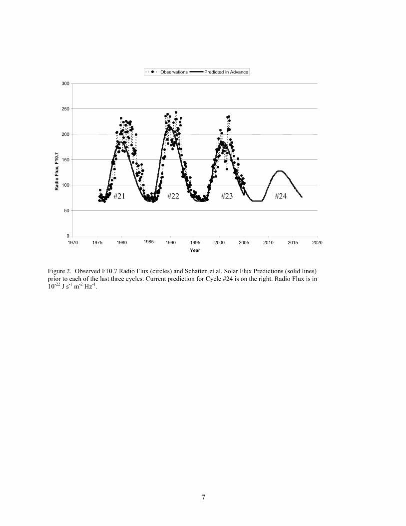
Figure 2. Observed F10.7 Radio Flux (circles) and Schatten et al. Solar Flux Predictions (solid lines)

prior to each of the last three cycles. Current prediction for Cycle #24 is on the right. Radio Flux is in

10-22 J s

-1 m-2 Hz

-1.

Figure 3. (Top) Drawing of coronal holes near the solar minimum of 1996 by Karen Harvey. Each pole shows a

large scale coronal hole, very typical of solar minimum conditions. (Bottom) Shown are a number of views of

current coronal hole maps (based on soft X-rays), with six different views of the Sun over the months between April

and August, 2005 time frame.

Figure 4. Calculated coronal magnetic field, based upon “source surface” calculations (Hoeksema, et al, 2005).

Top shows the coronal field in May 1994, and Bottom, in May 2005. The flattening of the “heliospheric current

sheet” (~ ±10 degrees) seen in the top figure supports a fully formed polar field which suppresses the undulations

in the sheet. In the current situation, the undulations are ~ ±30 degrees, which suggests polar fields are

insufficiently strong to suppress the current sheet curvatures.

Figures

6

19911976 2006

Figure 1: The polar field (10-6 T equal to Gauss) as observed at Wilcox Solar Observatory (WSO).

The solid line is the North polar field, and the dashed line, the Southern field. The yearly cycle as the

Earth moves ± 7 ¼ degrees in heliocentric latitude is a “noise” source. The recent polar field is

significantly lower than during the previous 3 solar cycles.

7

Figure 2. Observed F10.7 Radio Flux (circles) and Schatten et al. Solar Flux Predictions (solid lines)

prior to each of the last three cycles. Current prediction for Cycle #24 is on the right. Radio Flux is in

10-22 J s

-1 m-2 Hz

-1.

#21

0

50

100

150

200

250

300

1970 1975 1980 1985 1990 1995 2000 2005 2010 2015 2020 Year

Radio Flux, F10.7

Observations Predicted in Advance

#22 #24 #23

8

October, 1996 Coronal Hole Drawing,October, 1996 Coronal Hole Drawing,

Karen Harvey, using Karen Harvey, using KittKitt Peak He 10830 linePeak He 10830 line

April, May, 2005 STAR SOHO/MDI Coronal Hole Map

April - Aug 2005 STAR SOHO/MDI Coronal Hole Map

Figure 3. (Left) Drawing of coronal holes near the solar minimum of 1996 by Karen Harvey. Each pole shows a

large scale coronal hole, very typical of solar minimum conditions. (Right) Shown are a number of views of current

coronal hole maps (based on soft X-rays), with six different views of the Sun over the months between April and

August, 2005 time frame.

9

Figure 4. Calculated coronal magnetic field, based upon “source surface” calculations (Hoeksema, et al, 2005).

Top shows the coronal field in May 1994, and Bottom, in May 2005. The flattening of the “heliospheric current

sheet” (~ ±10 degrees) seen in the top figure supports a fully formed polar field which suppresses the undulations

in the sheet. In the current situation, the undulations are ~ ±30 degrees, which suggests polar fields are

insufficiently strong to suppress the current sheet curvatures.