Fair k-Center Clustering for Data Summarization

Fair k-Center Clustering for Data Summarization

Matthaus Kleindessner 1 Pranjal Awasthi 1 Jamie Morgenstern 2

AbstractIn data summarization we want to choose k proto-types in order to summarize a data set. We studya setting where the data set comprises several de-mographic groups and we are restricted to chooseki prototypes belonging to group i. A commonapproach to the problem without the fairness con-straint is to optimize a centroid-based clusteringobjective such as k-center. A natural extensionthen is to incorporate the fairness constraint intothe clustering problem. Existing algorithms fordoing so run in time super-quadratic in the size ofthe data set, which is in contrast to the standard k-center problem being approximable in linear time.In this paper, we resolve this gap by providing asimple approximation algorithm for the k-centerproblem under the fairness constraint with run-ning time linear in the size of the data set and k.If the number of demographic groups is small, theapproximation guarantee of our algorithm onlyincurs a constant-factor overhead.

1. IntroductionMachine learning (ML) algorithms have been rapidlyadopted in numerous human-centric domains, from person-alized advertising to lending to health care. Fast on the heelsof this ubiquity have come a whole host of concerning be-haviors from these algorithms: facial recognition has higheraccuracy on white, male faces (Buolamwini & Gebru, 2017);online advertisements suggesting arrest are shown more fre-quently to search queries that comprise a name primarilyassociated with minority groups (Sweeney, 2013); and crim-inal recidivism tools are likely to mislabel black low-riskdefendants as high-risk while mislabeling white high-riskdefendants as low-risk (Angwin et al., 2016). There are alsoseveral examples of unsavory ML behavior pertaining tounsupervised learning tasks, such as gender stereotypes in

1Department of Computer Science, Rutgers University, NJ2College of Computing, Georgia Tech, GA. Correspondence to:Matthaus Kleindessner <[email protected]>,Pranjal Awasthi <[email protected]>, Jamie Morgen-stern <[email protected]>.

word2vec embeddings (Bolukbasi et al., 2016). Most ofthe academic work on fairness in ML, however, has inves-tigated how to solve classification tasks subject to variousconstraints on the behavior of a classifier on different demo-graphic groups (e.g., Hardt et al., 2016; Zafar et al., 2017).

This paper adds to the literature on fair methods for unsu-pervised learning tasks (see Section 4 for related work). Weconsider the problem of data summarization (Hesabi et al.,2015) through the lens of algorithmic fairness. The goal ofdata summarization is to output a small but representativesubset of a data set. Think of an image database and a userentering a query that is matched by many images. Ratherthan presenting the user with all matching images, we onlywant to show a summary. In such an example, a data sum-mary can be quite unfair on a demographic group. Indeed,Google Images has been found to answer the query “CEO”with a much higher fraction of images of men compared tothe real-world fraction of male CEOs (Kay et al., 2015).

One approach to the problem of data summarization is pro-vided by centroid-based clustering, such as k-center (for-mally defined in Section 2) or k-medoid (Hastie et al., 2009,Section 14.3.10; sometimes referred to as k-median). Fora centroid-based clustering objective, an optimal clusteringof a data set S can be defined by k points c∗1, . . . , c

∗k ∈ S,

called centroids, such that the clusters are formed by assign-ing every s ∈ S to its closest centroid. Since the centroidsare good representatives of their clusters, the set of cen-troids can be used as a summary of S. This approach ofdata summarization via centroid-based clustering is usedin numerous domains, for example in text summarization(Moens et al., 1999) or robotics (Girdhar & Dudek, 2012).

If the data set S comprises several demographic groupsS1, . . . , Sm, we may consider c∗1, . . . , c

∗k to be a fair sum-

mary only if the groups are represented fairly: if in the realworld 70% of CEOs are male and we want to output tenimages for the query “CEO”, then three of the ten imagesshould show women. Formally, this can be encoded withone parameter kSi for every group Si. Our goal is then tominimize the clustering objective under the constraint thatkSi

many centroids belong to Si. A constraint of this formcan also enforce balanced summaries: even if in the realworld there are more male CEOs than female ones, we mightwant to output an equal number of male and female images

arX

iv:1

901.

0862

8v2

[st

at.M

L]

10

May

201

9


to reflect that gender is not definitional to the role of CEO.

Centroid-based clustering under such a constraint has beenstudied in the theoretical computer science literature (seeSections 2 and 4). However, existing approximation algo-rithms for this problem run in time ω(|S|2), while the uncon-strained k-center clustering problem can be approximatedin time linear in |S|. Since data summarization is particu-larly useful for massive data sets, such a slowdown may bepractically prohibitive. The contribution of this paper is topresent a simple approximation algorithm for k-center clus-tering under our fairness constraint with running time onlylinear in |S| and k. The improved running time comes at theprice of a worse guarantee on the approximation factor ifthe number of demographic groups is large. However, notethat in practical situations concerning fairness, the numberof groups is often quite small (e.g., when the groups encodegender or race). Furthermore, in our extensive numericalsimulations we never observed a large approximation factor,even when the number of groups was large (cf. Section 5),indicating the practical usefulness of our algorithm.

Outline of the paper In Section 2, we formally state thek-center and the fair k-center problem. In Section 3, wepresent our algorithm and provide a sketch of its analysis.The full proofs can be found in Appendix A. We discussrelated work in Section 4 and present a number of exper-iments in Section 5. Further experiments can be found inAppendix B. We conclude with a discussion in Section 6.

Notation For l ∈ N, we sometimes use [l] = 1, . . . , l.

2. Definition of k-Center and Fair k-CenterLet S be a finite data set and d : S × S → R≥0 be a metricon S. In particular, we assume d to satisfy the triangleinequality. The standard k-center clustering problem is theminimization problem

minimizeC=c1,...,ck⊆S

maxs∈S

d(s, C), (1)

where k ∈ N is a given parameter and d(s, C) =minc∈C d(s, c). Here, c1, . . . , ck are called centers. Any setof centers defines a clustering of S by assigning every s ∈ Sto its closest center. The k-center problem is NP-hard and isalso NP-hard to approximate to a factor better than 2 (Gon-zalez, 1985; Vazirani, 2001, Chapter 5). The famous greedystrategy of Gonzalez (1985) is a 2-approximation algorithmwith running time O(k|S|) if we assume that d can be eval-uated in constant time (this is the case, e.g., if a probleminstance is given via the distance matrix (d(s, s′))s,s′∈S).This greedy strategy chooses an arbitrary element of thedata set as first center and then iteratively selects the datapoint with maximum distance to the current set of centersas the next center to be added.

Algorithm 1 Approximation algorithm for (3)1: Input: metric d : S × S → R≥0; k ∈ N0; C ′0 ⊆ S2: Output: C = c1, . . . , ck ⊆ S3: set C = ∅4: for i = 1 to i = k5: choose ci ∈ argmaxs∈S d(s, C ∪ C ′0)6: set C = C ∪ ci7: return C

We consider a fair variant of the k-center problem as de-scribed in Section 1. Our variant also allows for the user tospecify a subset C0 ⊆ S that has to be included in the set ofcenters (think of the example of the image database and thecase that we always want to show five prespecified imagesas part of the summary). Assuming that S = ∪mi=1Si, whereS1, . . . Sm are the m demographic groups, the fair k-centerproblem can be stated as the minimization problem

minimizeC=c1,...,ck⊆S:

|C∩Si|=kSi, i=1,...,m

maxs∈S

d(s, C ∪ C0), (2)

where kSi∈ N0 with

∑mi=1 kSi

= k and C0 ⊆ S are given.By means of a partition matroid, the fair k-center problemcan be phrased as a matroid center problem, for which Chenet al. (2016) provide a 3-approximation algorithm using ma-troid intersection (e.g., Cook et al., 1998). Chen et al. (2016)do not discuss the running time of their algorithm, but it re-quires to sort all distances between elements in S and hencehas running time at least Ω(|S|2 log |S|). In our experimentsin Section 5 we observe a running time in Ω(|S|5/2).

3. A Linear-time Approximation AlgorithmIn this section, we present our approximation algorithm forthe minimization problem (2). It is a recursive algorithmwith respect to the number of groups m. To increase com-prehensibility, we first present the case of two groups andthen the general case of an arbitrary number of groups.

At several points, we will consider the standard (unfair) k-center problem (1) generalized to the case of initially givencenters C ′0 ⊆ S, that is

minimizeC=c1,...,ck⊆S

maxs∈S

d(s, C ∪ C ′0). (3)

We can adapt the greedy strategy of Gonzalez (1985) for(1) to problem (3) while maintaining its 2-approximationguarantee. For the sake of completeness, we provide thealgorithm as Algorithm 1 and state the following lemma:

Lemma 1. Algorithm 1 is a 2-approximation algorithm forthe unfair k-center problem (3) with running time O((k +|C ′0|)|S|), assuming d can be evaluated in constant time.


Algorithm 2 Approximation algorithm for (2) when m = 2

1: Input: metric d : S × S → R≥0; kS1, kS2

∈ N0

with kS1 + kS2 = k; C0 ⊆ S; group-membershipvector ∈ 1, 2|S| encoding membership in S1 or S2

2: Output: CA = cA1 , . . . , cAk ⊆ S3: run Algorithm 1 on S with k = kS1

+kS2andC ′0 = C0;

let CA = cA1 , . . . , cAk denote its output4:5: if |CA ∩ S1| = kS1 # implies |CA ∩ S2| = kS2

6: return CA

7: # we assume |CA∩S1| > kS1; otherwise we switch the

role of S1 and S2

8: form clusters L1, . . . , Lk, L′1, . . . , L

′|C0| by assigning

every s ∈ S to its closest center in CA ∪ C0

9: while |CA ∩ S1| > kS1and there exists Li with center

cAi ∈ S1 and y ∈ Li ∩ S2

10: replace center cAi with y by setting cAi = y11:12: if |CA ∩ S1| = kS1

# implies |CA ∩ S2| = kS2

13: return CA

14: let S′ = ∪i∈[k]:cAi ∈S1Li # we have S′ ⊆ S1

15: run Algorithm 1 on S′ ∪ C ′0 with k = kS1and C ′0 =

C0 ∪ (CA ∩ S2); let CA denote its output

16: return CA ∪ (CA ∩ S2) as well as (kS2− |CA ∩ S2|)

many arbitrary elements from S2

A proof of Lemma 1, similar in structure to a proof in Har-Peled (2011, Section 4.2) for the strategy of Gonzalez (1985)for problem (1), can be found in Appendix A.

3.1. Fair k-Center with Two Groups

Assume that S = S1∪S2. Our algorithm first runs Algo-rithm 1 for the unfair problem (3) with k = kS1

+ kS2and

C ′0 = C0. If we are lucky and Algorithm 1 picks kS1 manycenters from S1 and kS2 many centers from S2, our algo-rithm terminates. Otherwise, Algorithm 1 picks too manycenters from one group, say S1, and too few from S2. Wetry to decrease the number of centers in S1 by replacing anysuch a center with an element in its cluster belonging to S2.Once we have made all such available swaps, the remainingclusters with centers in S1 are entirely contained within S1.We then run Algorithm 1 on these clusters with k = kS1

andthe centers from S2 as well as C0 as initially given centers,and return both the centers from the recursive call (all in S1)and those from the initial call and the swapping in S2.

This algorithm is formally stated as Algorithm 2. The fol-lowing theorem states that it is a 5-approximation algorithmand that our analysis is tight—in general, Algorithm 2 doesnot achieve a better approximation factor.

Theorem 1. Algorithm 2 is a 5-approximation algorithmfor the fair k-center problem (2) with m = 2, but not a(5 − ε)-approximation algorithm for any ε > 0. It can beimplemented in time O((k + |C0|)|S|), assuming d can beevaluated in constant time.

Proof. Here we only present a sketch of the proof. Thefull proof can be found in Appendix A. For showing thatAlgorithm 2 is a 5-approximation algorithm, let r∗fair be theoptimal value of (2) and r∗ be the optimal value of (3) (forC ′0 = C0). Clearly, r∗ ≤ r∗fair. Let CA be the set of centersreturned by Algorithm 2. It is clear that CA compriseskS1 many elements from S1 and kS2 many elements fromS2. We need to show that minc∈CA∪C0

d(s, c) ≤ 5r∗fair forevery s ∈ S. Let CA be the output of Algorithm 1 whencalled in Line 3 of Algorithm 2. Since Algorithm 1 is a 2-approximation algorithm for (3) according to Lemma 1, wehave minc∈CA∪C0

d(s, c) ≤ 2r∗ ≤ 2r∗fair, s ∈ S. Assume

that |CA∩S1| > kS1 . It follows from the triangle inequalitythat after exchanging centers in the while-loop in Line 9 ofAlgorithm 2 we have minc∈CA∪C0

d(s, c) ≤ 4r∗fair, s ∈ S.

Assume that still |CA ∩ S1| > kS1. We only need to show

that minc∈CA∪C0d(s, c) ≤ 5r∗fair for s ∈ S′. Let C∗fair be

an optimal solution to (2). We split S′ into two subsetsS′ = S′a∪S′b, where S′a comprises all s ∈ S′ for which theclosest center in C∗fair ∪C0 is in S2 ∪C0. Using the triangleinequality we can show that minc∈CA∪C0

d(s, c) ≤ 5r∗fair,s ∈ S′a. We partition S′b into at most kS1

many clusterscorresponding to the closest center in C∗fair. Each of theseclusters has diameter not greater than 2r∗fair. If Algorithm 1in Line 15 of Algorithm 2 chooses one element from each ofthese clusters, we immediately have minc∈CA∪C0

d(s, c) ≤2r∗fair, s ∈ S′b. Otherwise, Algorithm 1 chooses an elementfrom S′a or two elements from the same cluster of S′b. Inboth cases, it follows from the greedy choice property ofAlgorithm 1 that minc∈CA∪C0

d(s, c) ≤ 5r∗fair, s ∈ S′b.A family of examples shows that Algorithm 2 is not a (5−ε)-approximation algorithm for any ε > 0.

3.2. Fair k-Center with Arbitrary Number of Groups

The main idea to handle an arbitrary number of groups m isthe same as for the case m = 2: we first run Algorithm 1.We then exchange centers for elements in their clusters insuch a way that the number of centers from a group Si comescloser to kSi

, which is the requested number of centers fromSi. If via exchanging centers we can actually hit kSi forevery group Si, we are done. Otherwise, we wish that,when no more exchanging is possible, we are left with asubset S′ ⊆ S that only comprises elements from m− 1 orfewer groups. Denote the set of these groups by G. We alsowish that for those groups not in G we have picked only therequested number of centers or fewer and we can considerthe groups not in G to have been “resolved”. If both are true,


L1 L2 L3

∈ S1 ∈ S1 ∈ S2

∈ S2

∈ S3

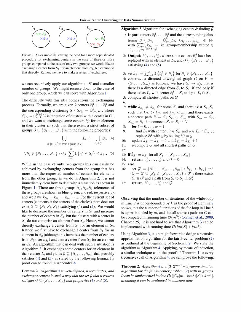
Figure 1. An example illustrating the need for a more sophisticatedprocedure for exchanging centers in the case of three or moregroups compared to the case of only two groups: we would like toexchange a center from S1 for an element from S3, but cannot dothat directly. Rather, we have to make a series of exchanges.

we can recursively apply our algorithm to S′ and a smallernumber of groups. We might recurse down to the case ofonly one group, which we can solve with Algorithm 1.

The difficulty with this idea comes from the exchangingprocess. Formally, we are given k centers cA1 , . . . , c

Ak and

the corresponding clustering S \ SC0= ∪ki=1Li, where

SC0 = ∪|C0|i=1L

′i is the union of clusters with a center in C0,

and we want to exchange some centers cAi for an elementin their cluster Li such that there exists a strict subset ofgroups G ( S1, . . . , Sm with the following properties:⋃

i∈[k]: cAi is from a group in G

Li ⊆⋃Si∈G

Si, (4)

∀Sj ∈ S1, . . . , Sm \ G :

k∑i=1

1cAi ∈ Sj

≤ kSj

. (5)

While in the case of only two groups this can easily beachieved by exchanging centers from the group that hasmore than the requested number of centers for elementsfrom the other group, as we do in Algorithm 2, it is notimmediately clear how to deal with a situation as shown inFigure 1. There are three groups S1, S2, S3 (elements ofthese groups are shown in blue, green, and red, respectively),and we have kS1

= kS2= kS3

= 1. For the current set ofcenters (elements at the centers of the circles) there does notexist G ( S1, S2, S3 satisfying (4) and (5). We wouldlike to decrease the number of centers in S1 and increasethe number of centers in S3, but the clusters with a center inS1 do not comprise an element from S3. Hence, we cannotdirectly exchange a center from S1 for an element in S3.Rather, we first have to exchange a center from S1 for anelement in S2 (although this increases the number of centersfrom S2 over kS2 ) and then a center from S2 for an elementin S3. An algorithm that can deal with such a situation isAlgorithm 3. It exchanges some centers for an element intheir cluster Li and yields G ( S1, . . . , Sm that provablysatisfies (4) and (5), as stated by the following lemma. Itsproof can be found in Appendix A.

Lemma 2. Algorithm 3 is well-defined, it terminates, andexchanges centers in such a way that the set G that it returnssatisfies G ( S1, . . . , Sm and properties (4) and (5).

Algorithm 3 Algorithm for exchanging centers & finding G1: Input: centers cA1 , . . . , c

Ak and the corresponding clus-

tering S \ SC0= ∪ki=1Li; kS1

, . . . , kSm∈ N0

with∑mi=1 kSi = k; group-membership vector ∈

1, . . . ,m|S\SC0|

2: Output: cA1 , . . . , cAk , where some centers cAi have beenreplaced with an element in Li, and G ( S1, . . . , Smsatisfying (4) and (5)

3: set kSj=∑ki=1 1

cAi ∈ Sj

for Sj ∈ S1, . . . , Sm

4: construct a directed unweighted graph G on V =S1, . . . , Sm as follows: we have Si → Sj , that isthere is a directed edge from Si to Sj , if and only ifthere exists Lt with center cAt ∈ Si and y ∈ Lt ∩ Sj

5: compute all shortest paths on G6:7: while kSj

6= kSjfor some Sj and there exist Sr, Ss

such that kSr > kSr and kSs < kSs and there existsa shortest path P = Sv0Sv1 · · ·Svw with Sv0 = Sr,Svw = Ss that connects Sr to Ss in G

8: for l = 0, . . . , w − 19: find Lt with center cAt ∈ Svl and y ∈ Lt ∩ Svl+1

;replace cAt with y by setting cAt = y

10: update kSr = kSr − 1 and kSs = kSs + 111: recompute G and all shortest paths on G12:13: if kSj

= kSjfor all Sj ∈ S1, . . . , Sm

14: return cA1 , . . . , cAk and G = ∅

15: else16: set G′ = Sj ∈ S1, . . . , Sm : kSj > kSj and

G = G′ ∪ Sj ∈ S1, . . . , Sm \ G′ : there existsSi ∈ G′ and a path from Si to Sj in G

17: return cA1 , . . . , cAk and G

Observing that the number of iterations of the while-loopin Line 7 is upper-bounded by k as the proof of Lemma 2shows, that the number of iterations of the for-loop in Line 8is upper-bounded by m, and that all shortest paths on G canbe computed in running time O(m3) (Cormen et al., 2009,Chapter 25), it is not hard to see that Algorithm 3 can beimplemented with running time O(km|S|+ km3).

Using Algorithm 3, it is straightforward to design a recursiveapproximation algorithm for the fair k-center problem (2)as outlined at the beginning of Section 3.2. We state thealgorithm as Algorithm 4. Applying, by means of induction,a similar technique as in the proof of Theorem 1 to every(recursive) call of Algorithm 4, we can prove the following:

Theorem 2. Algorithm 4 is a (3 ·2m−1−1)-approximationalgorithm for the fair k-center problem (2) with m groups.It can be implemented in timeO((|C0|m+km2)|S|+km4),assuming d can be evaluated in constant time.


Algorithm 4 Approximation alg. for (2) for arbitrary m1: Input: metric d : S × S → R≥0; kS1

, . . . , kSm∈

N0 with∑mi=1 kSi

= k; C0 ⊆ S; group-membershipvector ∈ 1, . . . ,m|S|

2: Output: CA = cA1 , . . . , cAk ⊆ S3: run Algorithm 1 on S with k =

∑mi=1 kSi

andC ′0 = C0; let CA = cA1 , . . . , cAk denote its output

4: if m = 15: return CA

6:7: form clusters L1, . . . , Lk, L

′1, . . . , L

′|C0| by assigning

every s ∈ S to its closest center in CA ∪ C0

8: apply Algorithm 3 to cA1 , . . . , cAk and ∪ki=1Li in or-

der to exchange some centers cAi and obtain G (S1, . . . , Sm

9: if G = ∅10: return CA

11:12: let S′ = ∪i∈[k]: cAi is from a group in G Li and

C ′ = cAi ∈ CA : cAi is from a group not in G; recur-sively call Algorithm 4, where:

• S′ ∪ C ′ ∪ C0 plays the role of S• we assign elements in C ′ ∪ C0 to an arbitrary group

in G and hence there are |G| < m many groupsSj1 , . . . , Sj|G|• the requested numbers of centers are kSj1

, . . . , kSj|G|

• C ′ ∪ C0 plays the role of initially given centers C0

let CR denote its output13: return CR ∪ C ′ as well as (kSj

− |C ′ ∩ Sj |) manyarbitrary elements from Sj for every group Sj not in G

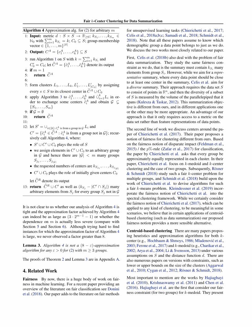
It is not clear to us whether our analysis of Algorithm 4 istight and the approximation factor achieved by Algorithm 4can indeed be as large as (3 · 2m−1 − 1) or whether thedependence on m is actually less severe (compare withSection 5 and Section 6). Although trying hard to findinstances for which the approximation factor of Algorithm 4is large, we never observed a factor greater than 8.

Lemma 3. Algorithm 4 is not a (8 − ε)-approximationalgorithm for any ε > 0 for (2) with m ≥ 3 groups.

The proofs of Theorem 2 and Lemma 3 are in Appendix A.

4. Related WorkFairness By now, there is a huge body of work on fair-ness in machine learning. For a recent paper providing anoverview of the literature on fair classification see Doniniet al. (2018). Our paper adds to the literature on fair methods

for unsupervised learning tasks (Chierichetti et al., 2017;Celis et al., 2018a;b;c; Samadi et al., 2018; Schmidt et al.,2018). Note that all these papers assume to know whichdemographic group a data point belongs to just as we do.We discuss the two works most closely related to our paper.

First, Celis et al. (2018b) also deal with the problem of fairdata summarization. They study the same fairness con-straint as we do, that is the summary must contain kSi

manyelements from group Si. However, while we aim for a repre-sentative summary, where every data point should be closeto at least one center in the summary, Celis et al. aim fora diverse summary. Their approach requires the data set Sto consist of points in Rn, and then the diversity of a subsetof S is measured by the volume of the parallelepiped that itspans (Kulesza & Taskar, 2012). This summarization objec-tive is different from ours, and in different applications oneor the other may be more appropriate. An advantage of ourapproach is that it only requires access to a metric on thedata set rather than feature representations of data points.

The second line of work we discuss centers around the pa-per of Chierichetti et al. (2017). Their paper proposes anotion of fairness for clustering different from ours. Basedon the fairness notion of disparate impact (Feldman et al.,2015) / the p%-rule (Zafar et al., 2017) for classification,the paper by Chierichetti et al. asks that every group beapproximately equally represented in each cluster. In theirpaper, Chierichetti et al. focus on k-medoid and k-centerclustering and the case of two groups. Subsequently, Rosner& Schmidt (2018) study such a fair k-center problem formultiple groups, and Schmidt et al. (2018) build upon thework of Chierichetti et al. to devise algorithms for sucha fair k-means problem. Kleindessner et al. (2019) incor-porate the fairness notion of Chierichetti et al. into thespectral clustering framework. While we certainly considerthe fairness notion of Chierichetti et al. (2017), which can beapplied to any kind of clustering, to be meaningful in somescenarios, we believe that in certain applications of centroid-based clustering (such as data summarization) our proposedfairness notion provides a more sensible alternative.

Centroid-based clustering There are many papers propos-ing heuristics and approximation algorithms for both k-center (e.g., Hochbaum & Shmoys, 1986; Mladenovic et al.,2003; Ferone et al., 2017) and k-medoid (e.g., Charikar et al.,2002; Arya et al., 2004; Li & Svensson, 2013) under variousassumptions on S and the distance function d. There arealso numerous papers on versions with constraints, such aslower or upper bounds on the size of the clusters (Aggarwalet al., 2010; Cygan et al., 2012; Rosner & Schmidt, 2018).

Most important to mention are the works by Hajiaghayiet al. (2010), Krishnaswamy et al. (2011) and Chen et al.(2016). Hajiaghayi et al. are the first that consider our fair-ness constraint (for two groups) for k-medoid. They present


a local search algorithm and prove it to be a constant-factorapproximation algorithm. Their work has been generalizedby Krishnaswamy et al., who consider k-medoid under theconstraint that the centers have to form an independent setin a given matroid. This kind of constraint contains our fair-ness constraint as a special case (for an arbitrary number ofgroups). Krishnaswamy et al. obtain a 16-approximation al-gorithm for this so-called matroid median problem based onrounding the solution of a linear programming relaxation.Subsequently, Chen et al. study the matroid center prob-lem. Using matroid intersection as black box, they obtain a3-approximation algorithm. Note that none of Hajiaghayiet al., Krishnaswamy et al. or Chen et al. discuss the run-ning time of their algorithm, except for arguing it to bepolynomial (see Section 2). We also mention the works byChakrabarty & Negahbani (2018), who provide a generaliza-tion of the matroid center problem and in doing so recoverthe result of Chen et al. (2016), and by Kale (2018), whostudies the matroid center problem in a streaming setting.

5. ExperimentsIn this section, we present a number of experiments1. Webegin with a motivating example on a small image data setillustrating that a summary produced by Algorithm 1 (i.e.,the standard greedy strategy for the unfair k-center problem)can be quite unfair. We also compare summaries producedby our algorithm to summaries produced by the method ofCelis et al. (2018b). We then investigate the approxima-tion factor of our algorithm on several artificial instanceswith known or computable optimal value of the fair k-centerproblem (2) and compare our algorithm to the one for thematroid center problem by Chen et al. (2016), both in termsof approximation factor / cost of output and running time.Next, on both synthetic and real data, we compare our al-gorithm in terms of the cost of its output to two baselineheuristics (with running time linear in |S| and k just as forour algorithm). Finally, we compare our algorithm to Al-gorithm 1 more systematically. We study the difference inthe costs of the outputs of our algorithm and Algorithm 1, aquantity one may refer to as price of fairness, and measurehow unfair the output of Algorithm 1 can be. In the follow-ing, all boxplots show results of 200 runs of an experiment.

5.1. Motivating Example and Comparison with Celiset al. (2018b)

Consider the 14 images2 of medical doctors shown in thefirst row of Figure 2. Assume we want to generate a sum-

1Python code is available on https://github.com/matthklein/fair k center clustering.

2All images were found on https://pexels.com, https://pixnio.com or https://commons.wikimedia.org and are in the public domain.

Algorithm 1 Our Algorithm Celis et al.

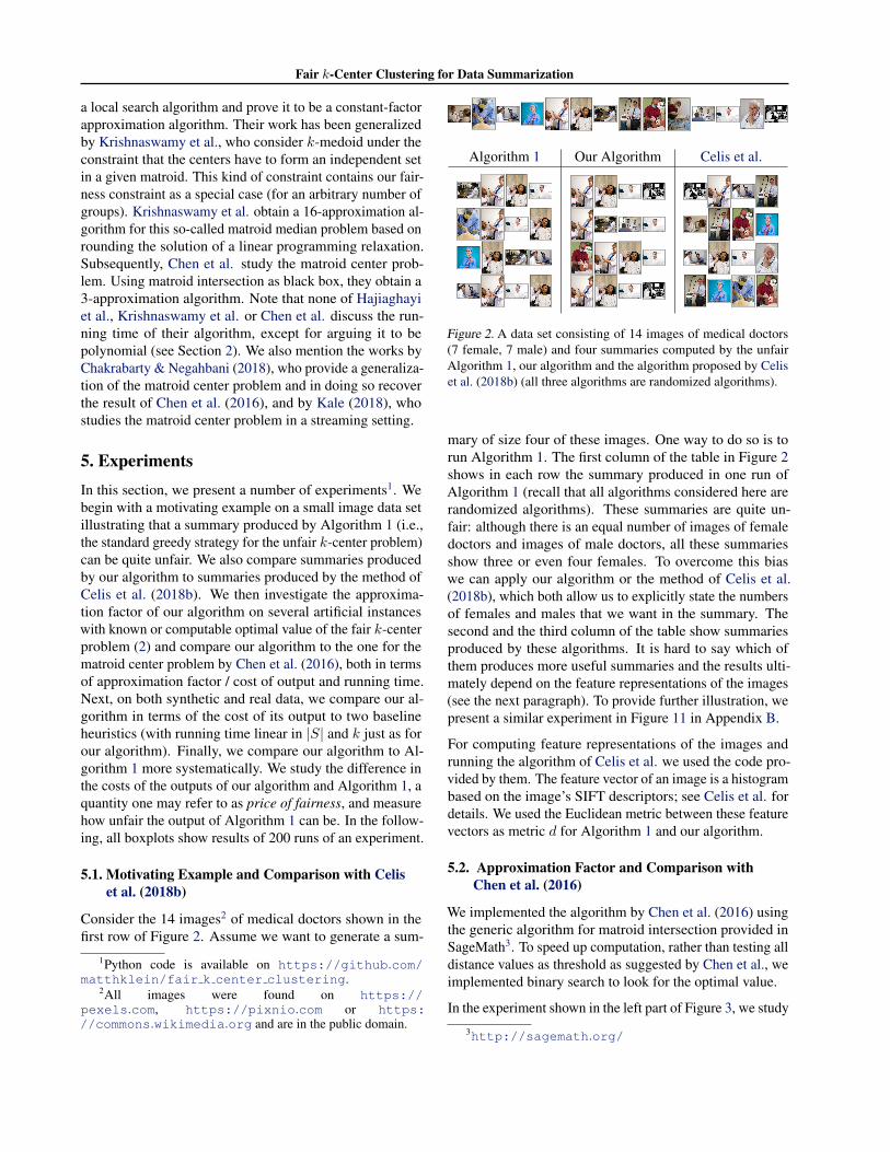
Figure 2. A data set consisting of 14 images of medical doctors(7 female, 7 male) and four summaries computed by the unfairAlgorithm 1, our algorithm and the algorithm proposed by Celiset al. (2018b) (all three algorithms are randomized algorithms).

mary of size four of these images. One way to do so is torun Algorithm 1. The first column of the table in Figure 2shows in each row the summary produced in one run ofAlgorithm 1 (recall that all algorithms considered here arerandomized algorithms). These summaries are quite un-fair: although there is an equal number of images of femaledoctors and images of male doctors, all these summariesshow three or even four females. To overcome this biaswe can apply our algorithm or the method of Celis et al.(2018b), which both allow us to explicitly state the numbersof females and males that we want in the summary. Thesecond and the third column of the table show summariesproduced by these algorithms. It is hard to say which ofthem produces more useful summaries and the results ulti-mately depend on the feature representations of the images(see the next paragraph). To provide further illustration, wepresent a similar experiment in Figure 11 in Appendix B.

For computing feature representations of the images andrunning the algorithm of Celis et al. we used the code pro-vided by them. The feature vector of an image is a histogrambased on the image’s SIFT descriptors; see Celis et al. fordetails. We used the Euclidean metric between these featurevectors as metric d for Algorithm 1 and our algorithm.

5.2. Approximation Factor and Comparison withChen et al. (2016)

We implemented the algorithm by Chen et al. (2016) usingthe generic algorithm for matroid intersection provided inSageMath3. To speed up computation, rather than testing alldistance values as threshold as suggested by Chen et al., weimplemented binary search to look for the optimal value.

In the experiment shown in the left part of Figure 3, we study

3http://sagemath.org/

https://github.com/matthklein/fair_k_center_clustering

https://github.com/matthklein/fair_k_center_clustering

https://pexels.com

https://pexels.com

https://pixnio.com

https://commons.wikimedia.org

https://commons.wikimedia.org

http://sagemath.org/


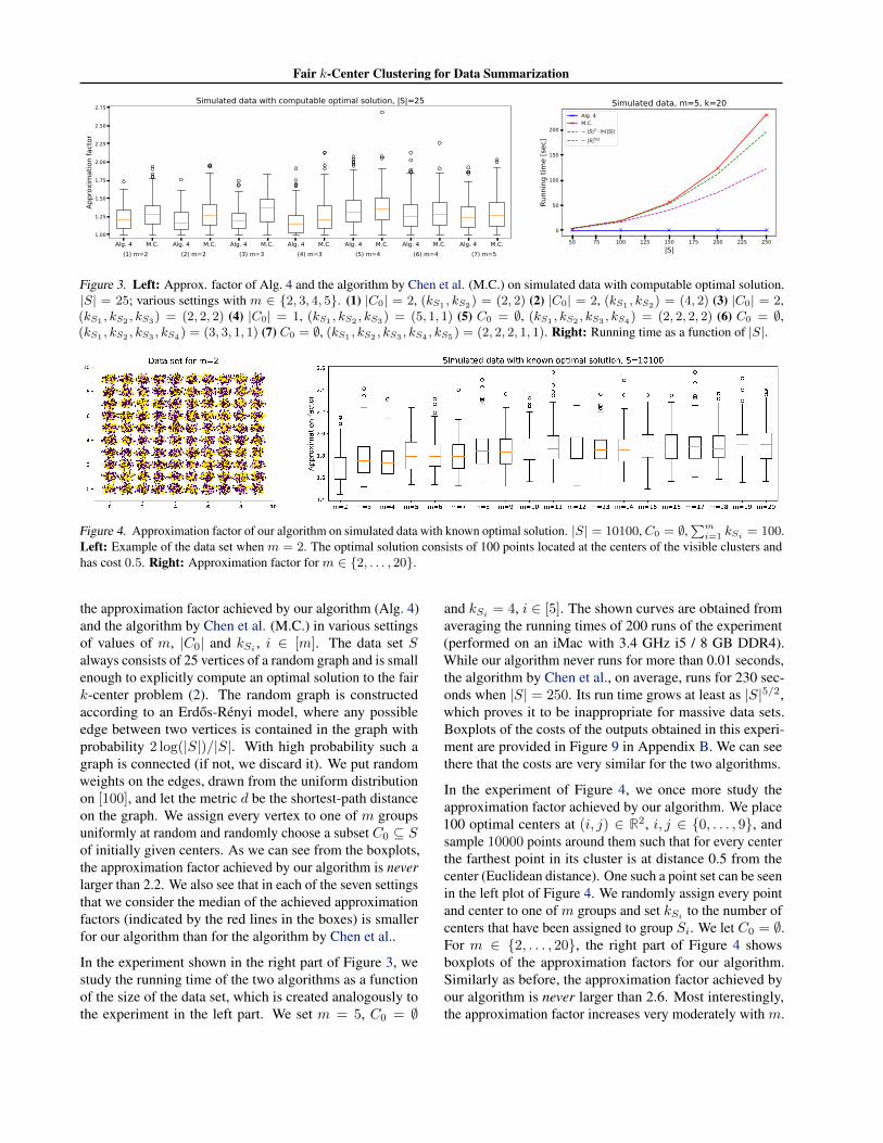
Figure 3. Left: Approx. factor of Alg. 4 and the algorithm by Chen et al. (M.C.) on simulated data with computable optimal solution.|S| = 25; various settings with m ∈ 2, 3, 4, 5. (1) |C0| = 2, (kS1 , kS2) = (2, 2) (2) |C0| = 2, (kS1 , kS2) = (4, 2) (3) |C0| = 2,(kS1 , kS2 , kS3) = (2, 2, 2) (4) |C0| = 1, (kS1 , kS2 , kS3) = (5, 1, 1) (5) C0 = ∅, (kS1 , kS2 , kS3 , kS4) = (2, 2, 2, 2) (6) C0 = ∅,(kS1 , kS2 , kS3 , kS4) = (3, 3, 1, 1) (7) C0 = ∅, (kS1 , kS2 , kS3 , kS4 , kS5) = (2, 2, 2, 1, 1). Right: Running time as a function of |S|.

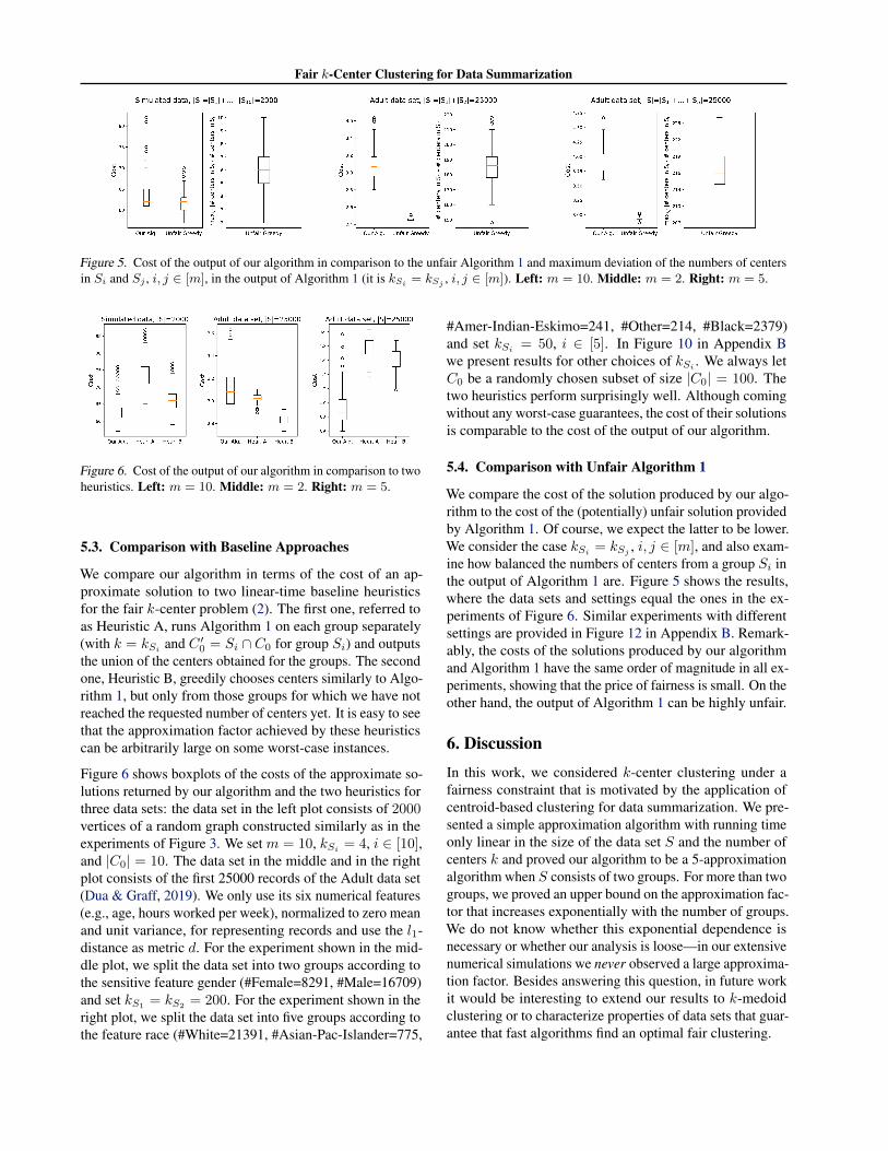
Figure 4. Approximation factor of our algorithm on simulated data with known optimal solution. |S| = 10100, C0 = ∅, ∑mi=1 kSi = 100.

Left: Example of the data set when m = 2. The optimal solution consists of 100 points located at the centers of the visible clusters andhas cost 0.5. Right: Approximation factor for m ∈ 2, . . . , 20.

the approximation factor achieved by our algorithm (Alg. 4)and the algorithm by Chen et al. (M.C.) in various settingsof values of m, |C0| and kSi , i ∈ [m]. The data set Salways consists of 25 vertices of a random graph and is smallenough to explicitly compute an optimal solution to the fairk-center problem (2). The random graph is constructedaccording to an Erdos-Renyi model, where any possibleedge between two vertices is contained in the graph withprobability 2 log(|S|)/|S|. With high probability such agraph is connected (if not, we discard it). We put randomweights on the edges, drawn from the uniform distributionon [100], and let the metric d be the shortest-path distanceon the graph. We assign every vertex to one of m groupsuniformly at random and randomly choose a subset C0 ⊆ Sof initially given centers. As we can see from the boxplots,the approximation factor achieved by our algorithm is neverlarger than 2.2. We also see that in each of the seven settingsthat we consider the median of the achieved approximationfactors (indicated by the red lines in the boxes) is smallerfor our algorithm than for the algorithm by Chen et al..

In the experiment shown in the right part of Figure 3, westudy the running time of the two algorithms as a functionof the size of the data set, which is created analogously tothe experiment in the left part. We set m = 5, C0 = ∅

and kSi= 4, i ∈ [5]. The shown curves are obtained from

averaging the running times of 200 runs of the experiment(performed on an iMac with 3.4 GHz i5 / 8 GB DDR4).While our algorithm never runs for more than 0.01 seconds,the algorithm by Chen et al., on average, runs for 230 sec-onds when |S| = 250. Its run time grows at least as |S|5/2,which proves it to be inappropriate for massive data sets.Boxplots of the costs of the outputs obtained in this experi-ment are provided in Figure 9 in Appendix B. We can seethere that the costs are very similar for the two algorithms.

In the experiment of Figure 4, we once more study theapproximation factor achieved by our algorithm. We place100 optimal centers at (i, j) ∈ R2, i, j ∈ 0, . . . , 9, andsample 10000 points around them such that for every centerthe farthest point in its cluster is at distance 0.5 from thecenter (Euclidean distance). One such a point set can be seenin the left plot of Figure 4. We randomly assign every pointand center to one of m groups and set kSi to the number ofcenters that have been assigned to group Si. We let C0 = ∅.For m ∈ 2, . . . , 20, the right part of Figure 4 showsboxplots of the approximation factors for our algorithm.Similarly as before, the approximation factor achieved byour algorithm is never larger than 2.6. Most interestingly,the approximation factor increases very moderately with m.


Figure 5. Cost of the output of our algorithm in comparison to the unfair Algorithm 1 and maximum deviation of the numbers of centersin Si and Sj , i, j ∈ [m], in the output of Algorithm 1 (it is kSi = kSj , i, j ∈ [m]). Left: m = 10. Middle: m = 2. Right: m = 5.

Figure 6. Cost of the output of our algorithm in comparison to twoheuristics. Left: m = 10. Middle: m = 2. Right: m = 5.

5.3. Comparison with Baseline Approaches

We compare our algorithm in terms of the cost of an ap-proximate solution to two linear-time baseline heuristicsfor the fair k-center problem (2). The first one, referred toas Heuristic A, runs Algorithm 1 on each group separately(with k = kSi

and C ′0 = Si ∩ C0 for group Si) and outputsthe union of the centers obtained for the groups. The secondone, Heuristic B, greedily chooses centers similarly to Algo-rithm 1, but only from those groups for which we have notreached the requested number of centers yet. It is easy to seethat the approximation factor achieved by these heuristicscan be arbitrarily large on some worst-case instances.

Figure 6 shows boxplots of the costs of the approximate so-lutions returned by our algorithm and the two heuristics forthree data sets: the data set in the left plot consists of 2000vertices of a random graph constructed similarly as in theexperiments of Figure 3. We set m = 10, kSi

= 4, i ∈ [10],and |C0| = 10. The data set in the middle and in the rightplot consists of the first 25000 records of the Adult data set(Dua & Graff, 2019). We only use its six numerical features(e.g., age, hours worked per week), normalized to zero meanand unit variance, for representing records and use the l1-distance as metric d. For the experiment shown in the mid-dle plot, we split the data set into two groups according tothe sensitive feature gender (#Female=8291, #Male=16709)and set kS1

= kS2= 200. For the experiment shown in the

right plot, we split the data set into five groups according tothe feature race (#White=21391, #Asian-Pac-Islander=775,

#Amer-Indian-Eskimo=241, #Other=214, #Black=2379)and set kSi = 50, i ∈ [5]. In Figure 10 in Appendix Bwe present results for other choices of kSi

. We always letC0 be a randomly chosen subset of size |C0| = 100. Thetwo heuristics perform surprisingly well. Although comingwithout any worst-case guarantees, the cost of their solutionsis comparable to the cost of the output of our algorithm.

5.4. Comparison with Unfair Algorithm 1

We compare the cost of the solution produced by our algo-rithm to the cost of the (potentially) unfair solution providedby Algorithm 1. Of course, we expect the latter to be lower.We consider the case kSi = kSj , i, j ∈ [m], and also exam-ine how balanced the numbers of centers from a group Si inthe output of Algorithm 1 are. Figure 5 shows the results,where the data sets and settings equal the ones in the ex-periments of Figure 6. Similar experiments with differentsettings are provided in Figure 12 in Appendix B. Remark-ably, the costs of the solutions produced by our algorithmand Algorithm 1 have the same order of magnitude in all ex-periments, showing that the price of fairness is small. On theother hand, the output of Algorithm 1 can be highly unfair.

6. DiscussionIn this work, we considered k-center clustering under afairness constraint that is motivated by the application ofcentroid-based clustering for data summarization. We pre-sented a simple approximation algorithm with running timeonly linear in the size of the data set S and the number ofcenters k and proved our algorithm to be a 5-approximationalgorithm when S consists of two groups. For more than twogroups, we proved an upper bound on the approximation fac-tor that increases exponentially with the number of groups.We do not know whether this exponential dependence isnecessary or whether our analysis is loose—in our extensivenumerical simulations we never observed a large approxima-tion factor. Besides answering this question, in future workit would be interesting to extend our results to k-medoidclustering or to characterize properties of data sets that guar-antee that fast algorithms find an optimal fair clustering.


AcknowledgementsThis research is supported by a Rutgers Research CouncilGrant and a Center for Discrete Mathematics and Theoreti-cal Computer Science (DIMACS) postdoctoral fellowship.

ReferencesAggarwal, G., Panigrahy, R., Feder, T., Thomas, D., Kentha-

padi, K., Khuller, S., and Zhu, A. Achieving anonymityvia clustering. ACM Transactions on Algorithms, 6(3):49:1–49:19, 2010.

Angwin, J., Larson, J., Mattu, S., and Kirch-ner, L. Propublica—machine bias, 2016.https://www.propublica.org/article/machine-bias-risk-assessments-in-criminal-sentencing.

Arya, V., Garg, N., Khandekar, R., Meyerson, A., Munagala,K., and Pandit, V. Local search heuristics for k-medianand facility location problems. SIAM Journal on Comput-ing, 33(3):544–562, 2004.

Bolukbasi, T., Chang, K.-W., Zou, J., Saligrama, V., andKalai, A. Man is to computer programmer as woman isto homemaker? Debiasing word embeddings. In NeuralInformation Processing Systems (NIPS), 2016.

Buolamwini, J. and Gebru, T. Gender shades: Intersectionalaccuracy disparities in commercial gender classification.In Conference on Fairness, Accountability, and Trans-parency (ACM FAT), 2017.

Celis, L. E., Huang, L., and Vishnoi, N. K. Multiwinnervoting with fairness constraints. In International JointConference on Artificial Intelligence (IJCAI), 2018a.

Celis, L. E., Keswani, V., Straszak, D., Deshpande,A., Kathuria, T., and Vishnoi, N. K. Fair anddiverse DPP-based data summarization. In Inter-national Conference on Machine Learning (ICML),2018b. Code available on https://github.com/DamianStraszak/FairDiverseDPPSampling.

Celis, L. E., Straszak, D., and Vishnoi, N. K. Rankingwith fairness constraints. In International Colloquium onAutomata, Languages and Programming (ICALP), 2018c.

Chakrabarty, D. and Negahbani, M. Generalized centerproblems with outliers. In International Colloquium onAutomata, Languages, and Programming (ICALP), 2018.

Charikar, M., Guha, S., Tardos, E., and Shmoys, D. B. Aconstant-factor approximation algorithm for the k-medianproblem. Journal of Computer and System Sciences, 65(1):129–149, 2002.

Chen, D. Z., Li, J., Liang, H., and Wang, H. Matroidand knapsack center problems. Algorithmica, 75:27–52,2016.

Chierichetti, F., Kumar, R., Lattanzi, S., and Vassilvitskii,S. Fair clustering through fairlets. In Neural InformationProcessing Systems (NIPS), 2017.

Cook, W. J., Cunningham, W. H., Pulleyblank, W. R., andSchrijver, A. Combinatorial Optimization. Wiley, 1998.

Cormen, T. H., Leiserson, C. E., Rivest, R. L., and Stein, C.Introduction to Algorithms. MIT Press, 3rd edition, 2009.

Cygan, M., Hajiaghayi, M., and Khuller, S. LP roundingfor k-centers with non-uniform hard capacities. In Sym-posium on Foundations of Computer Science (FOCS),2012.

Donini, M., Oneto, L., Ben-David, S., Shawe-Taylor, J., andPontil, M. Empirical risk minimization under fairnessconstraints. In Neural Information Processing Systems(NeurIPS), 2018.

Dua, D. and Graff, C. UCI machine learning reposi-tory, 2019. https://archive.ics.uci.edu/ml/datasets/adult.

Feldman, M., Friedler, S. A., Moeller, J., Scheidegger, C.,and Venkatasubramanian, S. Certifying and removingdisparate impact. In ACM International Conference onKnowledge Discovery and Data Mining (KDD), 2015.

Ferone, D., Festa, P., Napoletano, A., and Resende, M. G. C.A new local search for the p-center problem based on thecritical vertex concept. In International Conference onLearning and Intelligent Optimization (LION), 2017.

Girdhar, Y. and Dudek, G. Efficient on-line data summa-rization using extremum summaries. In InternationalConference on Robotics and Automation (ICRA), 2012.

Gonzalez, T. F. Clustering to minimize the maximum in-tercluster distance. Theoretical Computer Science, 38:293–306, 1985.

Hajiaghayi, M., Khandekar, R., and Kortsarz, G. The red-blue median problem and its generalization. In EuropeanSymposium on Algorithms (ESA), 2010.

Har-Peled, S. Geometric approximation algorithms. Ameri-can Mathematical Society, 2011.

Hardt, M., Price, E., and Srebro, N. Equality of opportunityin supervised learning. In Neural Information ProcessingSystems (NIPS), 2016.

Hastie, T., Tibshirani, R., and Friedman, J. The Elementsof Statistical Learning — Data Mining, Inference, andPrediction. Springer, 2nd edition, 2009.

https://www.propublica.org/article/machine-bias-risk-assessments-in-criminal-sentencing



https://github.com/DamianStraszak/FairDiverseDPPSampling

https://github.com/DamianStraszak/FairDiverseDPPSampling

https://archive.ics.uci.edu/ml/datasets/adult

https://archive.ics.uci.edu/ml/datasets/adult


Hesabi, Z. R., Tari, Z., Goscinski, A., Fahad, A., Khalil,I., and Queiroz, C. Data summarization techniques forbig data—a survey. In Handbook on Data Centers, pp.1109–1152. Springer, 2015.

Hochbaum, D. S. and Shmoys, D. B. A unified approach toapproximation algorithms for bottleneck problems. Jour-nal of the ACM, 33(3):533–550, 1986.

Kale, S. Small space stream summary for matroid center.arXiv:1810.06267 [cs.DS], 2018.

Kay, M., Matuszek, C., and Munson, S. A. Unequal repre-sentation and gender stereotypes in image search resultsfor occupations. In Conference on Human Factors inComputing Systems (CHI), 2015.

Kleindessner, M., Samadi, S., Awasthi, P., and Morgen-stern, J. Guarantees for spectral clustering with fairnessconstraints. In International Conference on MachineLearning (ICML), 2019.

Krishnaswamy, R., Kumar, A., Nagarajan, V., Sabharwal, Y.,and Saha, B. The matroid median problem. In Symposiumon Discrete Algorithms (SODA), 2011.

Kulesza, A. and Taskar, B. Determinantal point processesfor machine learning. Foundations and Trends in MachineLearning, 5:123–286, 2012.

Li, S. and Svensson, O. Approximating k-median viapseudo-approximation. In Symposium on the Theoryof Computing (STOC), 2013.

Mladenovic, N., Labbe, M., and Hansen, P. Solving thep-center problem with tabu search and variable neighbor-hood search. Networks, 42(1):48–64, 2003.

Moens, M.-F., Uyttendaele, C., and Dumortier, J. Abstract-ing of legal cases: The potential of clustering based onthe selection of representative objects. Journal of theAmerican Society for Information Science, 50(2):151–161, 1999.

Rosner, C. and Schmidt, M. Privacy preserving cluster-ing with constraints. In International Colloquium onAutomata, Languages, and Programming (ICALP), 2018.

Samadi, S., Tantipongpipat, U., Morgenstern, J., Singh,M., and Vempala, S. The price of fair PCA: One extradimension. In Neural Information Processing Systems(NeurIPS), 2018.

Schmidt, M., Schwiegelshohn, C., and Sohler, C. Fair core-sets and streaming algorithms for fair k-means clustering.arXiv:1812.10854 [cs.DS], 2018.

Sweeney, L. Discrimination in online ad delivery. Queue,11(3):10–29, 2013.

Vazirani, V. Approximation Algorithms. Springer, 2001.

Zafar, M. B., Valera, I., Rodriguez, M. G., and Gummadi,K. P. Fairness constraints: Mechanisms for fair classifi-cation. In International Conference on Artificial Intelli-gence and Statistics (AISTATS), 2017.

Appendix to Fair k-Center Clustering for Data Summarization

Appendix

A. Proofs

Proof of Lemma 1:

It is straightforward to see that Algorithm 1 can be implemented in time O((k + |C ′0|)|S|). We only need to show that it is a2-approximation algorithm for (3).

If k = 0, there is nothing to show, so assume that k ≥ 1. Let C = c1, . . . , ck be the output of Algorithm 1 andC∗ = c∗1, . . . , c∗k be an optimal solution to (3) with objective value r∗. Let s ∈ S be arbitrary. We need to show thatd(s, c) ≤ 2r∗ for some c ∈ C ∪ C ′0. If s ∈ C ∪ C ′0, there is nothing to show. So assume s /∈ C ∪ C ′0. If

C ′0 ∩ argminc∈C∗∪C′0

d(s, c) 6= ∅,

there exists c ∈ C ′0 with d(s, c) ≤ r∗ and we are done. Otherwise, let c∗i ∈ argminc∈C∗∪C′0 d(s, c) and hence d(s, c∗i ) ≤ r∗.We distinguish two cases:

• ∃ cj ∈ C with c∗i ∈ argminc∈C∗∪C′0 d(cj , c):

We have d(cj , c∗i ) ≤ r∗ and hence d(s, cj) ≤ d(s, c∗i ) + d(c∗i , cj) ≤ 2r∗.

• @ cj ∈ C with c∗i ∈ argminc∈C∗∪C′0 d(cj , c):

There must be c′ 6= c′′ ∈ C ∪ C ′0, where not both c′ and c′′ can be in C ′0, and c ∈ C∗ ∪ C ′0 such that

c ∈ argminc∈C∗∪C′0

d(c′, c) ∩ argminc∈C∗∪C′0

d(c′′, c).

Since d(c′, c) ≤ r∗ and (c′′, c∗) ≤ r∗, it follows that d(c′, c′′) ≤ d(c′, c) + d(c, c′′) ≤ 2r∗.

Without loss of generality, assume that in the execution of Algorithm 1, c′′ has been added to the set of centers afterc′ has been added. In particular, we have c′′ ∈ C and c′′ = cl for some l ∈ 1, . . . , k. Due to the greedy choice inLine 5 of the algorithm and since s has not been chosen by the algorithm, we have

2r∗ ≥ d(c′, c′′) ≥ minc∈c1,...,cl−1∪C′0

d(c′′, c) ≥ minc∈c1,...,cl−1∪C′0

d(s, c).

Proof of Theorem 1:

Again it is easy to see that Algorithm 2 can be implemented in time O((k + |C0|)|S|). We need to prove that it is a5-approximation algorithm, but not a (5− ε)-approximation algorithm for any ε > 0:

1. Algorithm 2 is a 5-approximation algorithm:

Let r∗fair be the optimal value of the fair problem (2) and r∗ be the optimal value of the unfair problem (3). Clearly,r∗ ≤ r∗fair. Let C∗fair = c(1)∗1 , . . . , c

(1)∗kS1

, c(2)∗1 , . . . , c

(2)∗kS2 with c

(1)∗1 , . . . , c

(1)∗kS1

∈ S1 and c(2)∗1 , . . . , c

(2)∗kS2

∈ S2

be an optimal solution to the fair problem (2) with cost r∗fair and CA = cA1 , . . . , cAk be the centers returned byAlgorithm 2. It is clear that Algorithm 2 returns kS1

many elements from S1 and kS2many elements from S2 and

hence CA = c(1)A1 , . . . , c(1)AkS1

, c(2)A1 , . . . , c

(2)AkS2 with c(1)A1 , . . . , c

(1)AkS1∈ S1 and c(2)A1 , . . . , c

(2)AkS2∈ S2. We need to

show thatmin

c∈CA∪C0

d(s, c) ≤ 5r∗fair, s ∈ S.


Let CA = cA1 , . . . , cAk be the output of Algorithm 1 when called in Line 3 of Algorithm 2. Since Algorithm 1 is a2-approximation algorithm for the unfair problem (3) according to Lemma 1, we have

minc∈CA∪C0

d(s, c) ≤ 2r∗ ≤ 2r∗fair, s ∈ S. (6)

If Algorithm 2 returns CA in Line 6, that is CA = CA, we are done. Otherwise assume, as in the algorithm, that|CA∩S1| > kS1 . Let cAi ∈ S1 be a center of clusterLi that we replace with y ∈ Li∩S2 and let y be an arbitrary elementin Li. Because of (6), we have d(cAi , y) ≤ 2r∗fair and d(cAi , y) ≤ 2r∗fair, and hence d(y, y) ≤ d(y, cAi )+d(cAi , y) ≤ 4r∗fairdue to the triangle inequality. Consequently, after the while-loop in Line 9, every s ∈ S is in distance of 4r∗fair orsmaller to the center of its cluster. In particular, we have

minc∈CA∪C0

d(s, c) ≤ 4r∗fair, s ∈ S,

and if Algorithm 2 returns CA in Line 13, we are done. Otherwise, we still have |CA ∩ S1| > kS1 after exchangingcenters in the while-loop in Line 9. Let S′ = ∪i∈[k]:cAi ∈S1

Li, that is the union of clusters with a center cAi ∈ S1. Sincethere is no more center in S1 that we can exchange for an element in S2, we have S′ ⊆ S1. Let S′′ = ∪i∈[k]:cAi ∈S2

Li

be the union of clusters with a center cAi ∈ S2 and SC0= L′1 ∪ . . . ∪ L′|C0| be the union of clusters with a center in C0.

Then we have S = S′ ∪S′′ ∪SC0. We have CA ∩ S2 ⊆ CA and

minc∈CA∪C0

d(s, c) ≤ minc∈(CA∩S2)∪C0

d(s, c) ≤ 4r∗fair, s ∈ S′′ ∪ SC0 . (7)

Hence we only need to show that minc∈CA∪C0d(s, c) ≤ 5r∗fair for every s ∈ S′. We split S′ into two subsets

S′ = S′a∪S′b, where

S′a =

s ∈ S′ : argmin

c∈C∗fair∪C0

d(s, c) ∩ (C0 ∪ S2) 6= ∅

and S′b = S′ \ S′a. For every s ∈ S′a there is c ∈ (C0 ∪ S2) ⊆ (S′′ ∪ SC0) with d(s, c) ≤ r∗fair and it follows from (7)

and the triangle inequality that

minc∈CA∪C0

d(s, c) ≤ minc∈(CA∩S2)∪C0

d(s, c) ≤ 5r∗fair, s ∈ S′a. (8)

It remains to show that minc∈CA∪C0d(s, c) ≤ 5r∗fair for every s ∈ S′b. For every s ∈ S′b there exists

c ∈ c(1)∗1 , . . . , c(1)∗kS1 with d(s, c) ≤ r∗fair. We can write S′b = ∪kS1

j=1s ∈ S′b : d(s, c(1)∗j ) ≤ r∗fair (some of the

sets in this union might be empty, but that does not matter). Note that for every j ∈ 1, . . . , kS1 we have

d(s, s′) ≤ 2r∗fair, s, s′ ∈s ∈ S′b : d(s, c

(1)∗j ) ≤ r∗fair

, (9)

due to the triangle inequality. It is

S′ = S′a ∪ S′b = S′a ∪kS1⋃j=1

s ∈ S′b : d(s, c

(1)∗j ) ≤ r∗fair

and when, in Line 15 of Algorithm 2, we run Algorithm 1 on S′ ∪ C ′0 with k = kS1 and initial centers C ′0 =

C0 ∪ (CA ∩ S2), one of the following three cases has to happen (we denote the centers returned by Algorithm 1 byCA = c(1)A1 , . . . , c

(1)AkS1):

• For every j ∈ 1, . . . , kS1 there exists j′ ∈ 1, . . . , kS1 such that c(1)Aj′ ∈ s ∈ S′b : d(s, c(1)∗j ) ≤ r∗fair. In this

case it immediately follows from (9) that

minc∈CA∪C0

d(s, c) ≤ minc∈CA

d(s, c) ≤ 2r∗fair, s ∈ S′b.


1+ δ4

1+δ

2 1

1+ δ22

1-δ

1

2

δ2

100

2

4

f1

m1

f2

m2

f3

m3

m4m5

m6

f4

f5

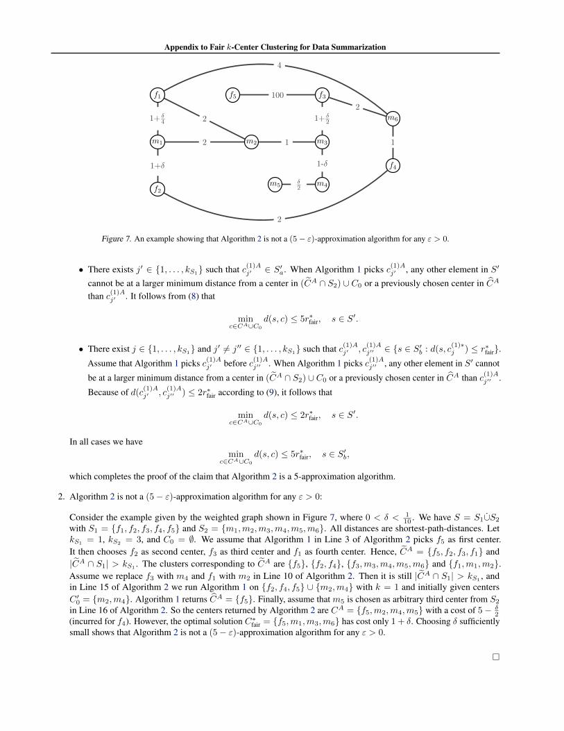
Figure 7. An example showing that Algorithm 2 is not a (5− ε)-approximation algorithm for any ε > 0.

• There exists j′ ∈ 1, . . . , kS1 such that c(1)Aj′ ∈ S′a. When Algorithm 1 picks c(1)Aj′ , any other element in S′

cannot be at a larger minimum distance from a center in (CA ∩ S2) ∪ C0 or a previously chosen center in CA

than c(1)Aj′ . It follows from (8) that

minc∈CA∪C0

d(s, c) ≤ 5r∗fair, s ∈ S′.

• There exist j ∈ 1, . . . , kS1 and j′ 6= j′′ ∈ 1, . . . , kS1

such that c(1)Aj′ , c(1)Aj′′ ∈ s ∈ S′b : d(s, c

(1)∗j ) ≤ r∗fair.

Assume that Algorithm 1 picks c(1)Aj′ before c(1)Aj′′ . When Algorithm 1 picks c(1)Aj′′ , any other element in S′ cannot

be at a larger minimum distance from a center in (CA ∩ S2) ∪ C0 or a previously chosen center in CA than c(1)Aj′′ .

Because of d(c(1)Aj′ , c

(1)Aj′′ ) ≤ 2r∗fair according to (9), it follows that

minc∈CA∪C0

d(s, c) ≤ 2r∗fair, s ∈ S′.

In all cases we havemin

c∈CA∪C0

d(s, c) ≤ 5r∗fair, s ∈ S′b,

which completes the proof of the claim that Algorithm 2 is a 5-approximation algorithm.

2. Algorithm 2 is not a (5− ε)-approximation algorithm for any ε > 0:

Consider the example given by the weighted graph shown in Figure 7, where 0 < δ < 110 . We have S = S1∪S2

with S1 = f1, f2, f3, f4, f5 and S2 = m1,m2,m3,m4,m5,m6. All distances are shortest-path-distances. LetkS1

= 1, kS2= 3, and C0 = ∅. We assume that Algorithm 1 in Line 3 of Algorithm 2 picks f5 as first center.

It then chooses f2 as second center, f3 as third center and f1 as fourth center. Hence, CA = f5, f2, f3, f1 and|CA ∩ S1| > kS1

. The clusters corresponding to CA are f5, f2, f4, f3,m3,m4,m5,m6 and f1,m1,m2.Assume we replace f3 with m4 and f1 with m2 in Line 10 of Algorithm 2. Then it is still |CA ∩ S1| > kS1 , andin Line 15 of Algorithm 2 we run Algorithm 1 on f2, f4, f5 ∪ m2,m4 with k = 1 and initially given centersC ′0 = m2,m4. Algorithm 1 returns CA = f5. Finally, assume that m5 is chosen as arbitrary third center from S2

in Line 16 of Algorithm 2. So the centers returned by Algorithm 2 are CA = f5,m2,m4,m5 with a cost of 5− δ2

(incurred for f4). However, the optimal solution C∗fair = f5,m1,m3,m6 has cost only 1 + δ. Choosing δ sufficientlysmall shows that Algorithm 2 is not a (5− ε)-approximation algorithm for any ε > 0.


Proof of Lemma 2:

We want to show three things:

1. Algorithm 3 is well-defined:

If the condition of the while-loop in Line 7 is true, there exists a shortest path P = Sv0Sv1 · · ·Svw with Sv0 = Sr,Svw = Ss that connects Sr to Ss in G. Since P is a shortest path, all Svi are distinct. By the definition of G, forevery l = 0, . . . , w − 1 there exists Lt with center cAt ∈ Svl and y ∈ Lt ∩ Svl+1

. Hence, the for-loop in Line 8 is welldefined.

2. Algorithm 3 terminates:

Let, at the beginning of the execution of Algorithm 3 in Line 3, H1 = Sj ∈ S1, . . . , Sm : kSj = kSj,H2 = Sj ∈ S1, . . . , Sm : kSj

> kSj and H3 = Sj ∈ S1, . . . , Sm : kSj

< kSj. For Sj ∈ H1, kSj

neverchanges during the execution of the algorithm. For Sj ∈ H2, kSj

never increases during the execution of the algorithmand decreases at most until it equals kSj

. For Sj ∈ H3, kSjnever decreases during the execution of the algorithm and

increases at most until it equals kSj. In every iteration of the while-loop, there is Sj ∈ H3 for which kSj

increases byone. It follows that the number of iterations of the while-loop is upper-bounded by k.

3. Algorithm 3 exchanges centers in such a way that the set G that it returns satisfies G ( S1, . . . , Sm and properties (4)and (5):

Note that throughout the execution of Algorithm 3 we have kSj =∑ki=1 1

cAi ∈ Sj

for the current centers cA1 , . . . , c

Ak .

If the condition of the if-statement in Line 13 is true, then G = ∅ and (4) and (5) are satisfied.

Assume that the condition of the if-statement in Line 13 is not true. Clearly, the set G returned by Algorithm 3satisfies (5). Since the condition of the if-statement in Line 13 is not true, there exist Sj with kSj

> kSjand Si with

kSi< kSi

. We have Sj ∈ G, but since the condition of the while-loop in Line 7 is not true, we cannot have Si ∈ G.This shows that G ( S1, . . . , Sm. We need to show that (4) holds. Let Lh be a cluster with center cAh ∈ Sf for someSf ∈ G and assume it contained an element o ∈ Sf ′ with Sf ′ /∈ G. But then we had a path from Sf to Sf ′ in G. IfSf ∈ G′, this is an immediate contradiction to Sf ′ /∈ G. If Sf /∈ G′, since Sf ∈ G, there exists Sg ∈ G′ such that thereis a path from Sg to Sf . But then there is also a path from Sg to Sf ′ , which is a contradiction to Sf ′ /∈ G.

Proof of Theorem 2:

For showing that Algorithm 4 is a (3 · 2m−1 − 1)-approximation algorithm let r∗fair be the optimal value of problem (2) andC∗fair be an optimal solution with cost r∗fair. Let CA be the centers returned by Algorithm 4. A simple proof by inductionover m shows that CA actually comprises kSi

many elements from every group Si. We need to show that

minc∈CA∪C0

d(s, c) ≤ (3 · 2m−1 − 1)r∗fair, s ∈ S. (10)

Let T be the total number of calls of Algorithm 4, that is we have one initial call and T − 1 recursive calls. Since witheach recursive call the number of groups is decreased by at least one, we have T ≤ m. For 1 ≤ j ≤ T , let S(j) be the dataset in the j-th call of Algorithm 4. We additionally set S(T+1) = ∅. We have S(1) = S and S(j) ⊇ S(j+1), 1 ≤ j ≤ T .For 1 ≤ j < T , let G(j) be the set of groups in G returned by Algorithm 3 in Line 8 in the j-th call of Algorithm 4. Ifin the T -th call of Algorithm 4 the algorithm terminates from Line 10 (note that in this case we must have T < m), wealso let G(T ) = ∅ be the set of groups in G returned by Algorithm 3 in the T -th call. Otherwise we leave G(T ) undefined.Setting G(0) = S1, . . . , Sm, we have G(j) ) G(j+1) for all j such that G(j+1) is defined. For 1 ≤ j < T , let Cj bethe set of centers returned by Algorithm 3 in Line 8 in the j-th call of Algorithm 4 that belong to a group not in G(j) (inAlgorithm 4, the set of these centers is denoted by C ′). We analogously define CT if in the T -th call of Algorithm 4 thealgorithm terminates from Line 10. Note that the centers in Cj are comprised in the final output CA of Algorithm 4, that is


Cj ⊆ CA for 1 ≤ j < T or 1 ≤ j ≤ T . As always, C0 denotes the set of centers that are given initially (for the initial callof Algorithm 4). Note that in the j-th call of Algorithm 4 the set of initially given centers is C0 ∪

⋃j−1l=1 Cl.

We first prove by induction that for all j ≥ 1 such that G(j) is defined, that is 1 ≤ j < T or 1 ≤ j ≤ T , we have

minc∈C0∪

⋃jl=1 Cl

d(s, c) ≤ (2j+1 + 2j − 2)r∗fair, s ∈(S(j) \ S(j+1)

)∪(C0 ∪

j⋃l=1

Cl

). (11)

Base case j = 1: In the first call of Algorithm 4, Algorithm 1, when called in Line 3 of Algorithm 4, returns an approximatesolution to the unfair problem (3). Let r∗ ≤ r∗fair be the optimal cost of (3). Since Algorithm 1 is a 2-approximationalgorithm for (3) according to Lemma 1, after Line 3 of Algorithm 4 we have

minc∈CA∪C0

d(s, c) ≤ 2r∗ ≤ 2r∗fair, s ∈ S.

Let cAi ∈ CA be a center and s1, s2 ∈ Li be two points in its cluster. It follows from the triangle inequality thatd(s1, s2) ≤ d(s1, c

Ai ) + d(cAi , s2) ≤ 4r∗fair. Hence, after running Algorithm 3 in Line 8 of Algorithm 4 and exchanging

some of the centers in CA, we have d(s, c(s)) ≤ 4r∗fair for every s ∈ S, where c(s) denotes the center of its cluster. Inparticular,

minc∈C0∪C1

d(s, c) ≤ (21+1 + 21 − 2)r∗fair = 4r∗fair

for all s ∈ S for which its center c(s) is in C0 or in a group not in G(1), that is for s ∈ (S(1) \ S(2)) ∪ (C0 ∪ C1).

Inductive step j 7→ j + 1: Recall property (4) of a set G returned by Algorithm 3. Consequently, S(j+1) only comprisesitems in a group in G(j) and, additionally, the given centers C0 ∪

⋃jl=1 Cl.

We split S(j+1) into two subsets S(j+1) = S(j+1)a ∪S(j+1)

b , where

S(j+1)a =

s ∈ S(j+1) : argminc∈C∗fair∪C0

d(s, c) ∩

C0 ∪⋃

W∈S1,...,Sm\G(j)

W

6= ∅

and S(j+1)b = S(j+1) \ S(j+1)

a . For every s ∈ S(j+1)a there exists

c ∈ C0 ∪⋃

W∈S1,...,Sm\G(j)

W ⊆(S \ S(j+1)

)∪(C0 ∪

j⋃l=1

Cl

)

with d(s, c) ≤ r∗fair. It follows from the inductive hypothesis that there exists c′ ∈ C0 ∪⋃jl=1 Cl with d(c, c′) ≤

(2j+1 + 2j − 2)r∗fair and consequently

d(s, c′) ≤ d(s, c) + d(c, c′) ≤ r∗fair + (2j+1 + 2j − 2)r∗fair = (2j+1 + 2j − 1)r∗fair.

Hence,

minc∈C0∪

⋃jl=1 Cl

d(s, c) ≤ (2j+1 + 2j − 1)r∗fair, s ∈ S(j+1)a . (12)

For every s ∈ S(j+1)b there exists c ∈ C∗fair ∩

⋃W∈G(j) W with d(s, c) ≤ r∗fair. Let C∗fair ∩

⋃W∈G(j) W = c∗1, . . . , c∗k with

k =∑W∈G(j) kW , where kW is the number of requested centers from group W . We can write

S(j+1)b =

k⋃l=1

s ∈ S(j+1)

b : d(s, c∗l ) ≤ r∗fair

,


where some of the sets in this union might be empty, but that does not matter. Note that for every l = 1, . . . , k we have

d(s, s′) ≤ 2r∗fair, s, s′ ∈s ∈ S(j+1)


(13)

due to the triangle inequality. It is

S(j+1) = S(j+1)a ∪ S(j+1)

b = S(j+1)a ∪

k⋃l=1

s ∈ S(j+1)


and when, in Line 3 of Algorithm 4, we run Algorithm 1 on S(j+1) with k = k and initial centers C0 ∪

⋃jl=1 Cl, one of the

following three cases has to happen (we denote the centers returned by Algorithm 1 in this (j + 1)-th call of Algorithm 4 byFA = fA1 , . . . , fAk and assume that for 1 ≤ l < l′ ≤ k Algorithm 1 has chosen fAl before fAl′ ):

• For every l ∈ 1, . . . , k there exists l′ ∈ 1, . . . , k such that fAl′ ∈ s ∈ S(j+1)b : d(s, c∗l ) ≤ r∗fair. In this case it

immediately follows that

minc∈FA

d(s, c) ≤ 2r∗fair, s ∈ S(j+1)b ,

and using (12) we obtain

minc∈C0∪

⋃jl=1 Cl∪FA

d(s, c) ≤ (2j+1 + 2j − 1)r∗fair, s ∈ S(j+1).

• There exists l′ ∈ 1, . . . , k such that fAl′ ∈ S(j+1)a . When Algorithm 1 picks fAl′ , any other element in S(j+1) cannot

be at a larger minimum distance from a center in C0 ∪⋃jl=1 Cl or an already chosen center in fAl′ , . . . , fAl′−1 than

fAl′ . It follows from (12) that

minc∈C0∪

⋃jl=1 Cl∪FA

d(s, c) ≤ (2j+1 + 2j − 1)r∗fair, s ∈ S(j+1).

• There exist l ∈ 1, . . . , k and l′, l′′ ∈ 1, . . . , k with l′ < l′′ such that fAl′ , fAl′′ ∈ s ∈ S

(j+1)b : d(s, c∗l ) ≤ r∗fair.

When Algorithm 1 picks fAl′′ , any other element in S(j+1) cannot be at a larger minimum distance from a center inC0 ∪

⋃jl=1 Cl or an already chosen center in fAl′ , . . . , fAl′′−1 than fAl′′ . Because of d(fAl′ , f

Al′′) ≤ 2r∗fair according to

(13), it follows that

minc∈C0∪

⋃jl=1 Cl∪FA

d(s, c) ≤ 2r∗fair ≤ (2j+1 + 2j − 1)r∗fair, s ∈ S(j+1).

In any case, we have

minc∈C0∪

⋃jl=1 Cl∪FA

d(s, c) ≤ (2j+1 + 2j − 1)r∗fair, s ∈ S(j+1). (14)

Similarly to the base case, it follows from the triangle inequality that after running Algorithm 3 in Line 8 of Algorithm 4 andexchanging some of the centers in FA, we have

d(s, c(s)) ≤ 2(2j+1 + 2j − 1)r∗fair = (2j+2 + 2j+1 − 2)r∗fair

for every s ∈ S(j+1), where c(s) denotes the center of its cluster. In particular, we have

minc∈C0∪

⋃j+1l=1 Cl

d(s, c) ≤ (2j+2 + 2j+1 − 2)r∗fair, s ∈(S(j+1) \ S(j+2)

)∪(C0 ∪

j+1⋃l=1

Cl

),

and this completes the proof of (11).


1

2− δ

δ

1 + 3δ2 4 + δ

2 4

2− δ

δ

1

1 + δ

4

12

8

f1

m1

m5

m2

f2 f3 z2

z1

m3

f4

m4

m6

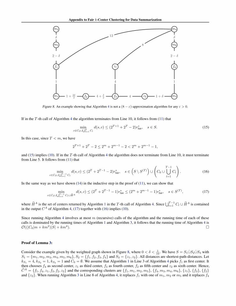
Figure 8. An example showing that Algorithm 4 is not a (8− ε)-approximation algorithm for any ε > 0.

If in the T -th call of Algorithm 4 the algorithm terminates from Line 10, it follows from (11) that

minc∈C0∪

⋃Tl=1 Cl

d(s, c) ≤ (2T+1 + 2T − 2)r∗fair, s ∈ S. (15)

In this case, since T < m, we have

2T+1 + 2T − 2 ≤ 2m + 2m−1 − 2 < 2m + 2m−1 − 1,

and (15) implies (10). If in the T -th call of Algorithm 4 the algorithm does not terminate from Line 10, it must terminatefrom Line 5. It follows from (11) that

minc∈C0∪

⋃T−1l=1 Cl

d(s, c) ≤ (2T + 2T−1 − 2)r∗fair, s ∈(S \ S(T )

)∪(C0 ∪

T−1⋃l=1

Cl

). (16)

In the same way as we have shown (14) in the inductive step in the proof of (11), we can show that

minc∈C0∪

⋃T−1l=1 Cl∪HA

d(s, c) ≤ (2T + 2T−1 − 1)r∗fair ≤ (2m + 2m−1 − 1)r∗fair, s ∈ S(T ), (17)

where HA is the set of centers returned by Algorithm 1 in the T -th call of Algorithm 4. Since⋃T−1l=1 Cl ∪ HA is contained

in the output CA of Algorithm 4, (17) together with (16) implies (10).

Since running Algorithm 4 involves at most m (recursive) calls of the algorithm and the running time of each of thesecalls is dominated by the running times of Algorithm 1 and Algorithm 3, it follows that the running time of Algorithm 4 isO((|C0|m+ km2)|S|+ km4).

Proof of Lemma 3:

Consider the example given by the weighted graph shown in Figure 8, where 0 < δ < 110 . We have S = S1∪S2∪S3 with

S1 = m1,m2,m3,m4,m5,m6, S2 = f1, f2, f3, f4 and S3 = z1, z2. All distances are shortest-path-distances. LetkS1

= 4, kS2= 1, kS3

= 1 and C0 = ∅. We assume that Algorithm 1 in Line 3 of Algorithm 4 picks f1 as first center. Itthen chooses f4 as second center, z1 as third center, f3 as fourth center, f2 as fifth center and z2 as sixth center. Hence,CA = f1, f4, z1, f3, f2, z2 and the corresponding clusters are f1,m1,m2,m5, f4,m3,m4,m6, z1, f3, f2and z2. When running Algorithm 3 in Line 8 of Algorithm 4, it replaces f1 with one of m1, m2 or m5 and it replaces f4


with one of m3, m4 or m6. Assume that it replaces f1 with m2 and f4 with m4. Algorithm 3 then returns G = S2, S3and when recursively calling Algorithm 4 in Line 12, we have S′ = f2, f3, z1, z2 and C ′ = m2,m4. In the recursivecall, the given centers are C ′ and Algorithm 1 chooses f3 and f2. The corresponding clusters are f3, z1, z2, f2, m2and m4. When running Algorithm 3 with clusters f3, z1, z2 and f2, it replaces f3 with either z1 or z2 and returnsG = ∅, that is afterwards we are done. Assume Algorithm 3 replaces f3 with z2. Then the centers returned by Algorithm 4are z2, f2,m2,m4 and two arbitrary elements from S1, which we assume to be m5 and m6. These centers have a cost of 8(incurred for z1). However, an optimal solution such as C∗fair = m1,m2,m3,m4, f3, z1 has cost only 1 + 3δ

2 . Choosing δsufficiently small shows that Algorithm 4 is not a (8− ε)-approximation algorithm for any ε > 0.

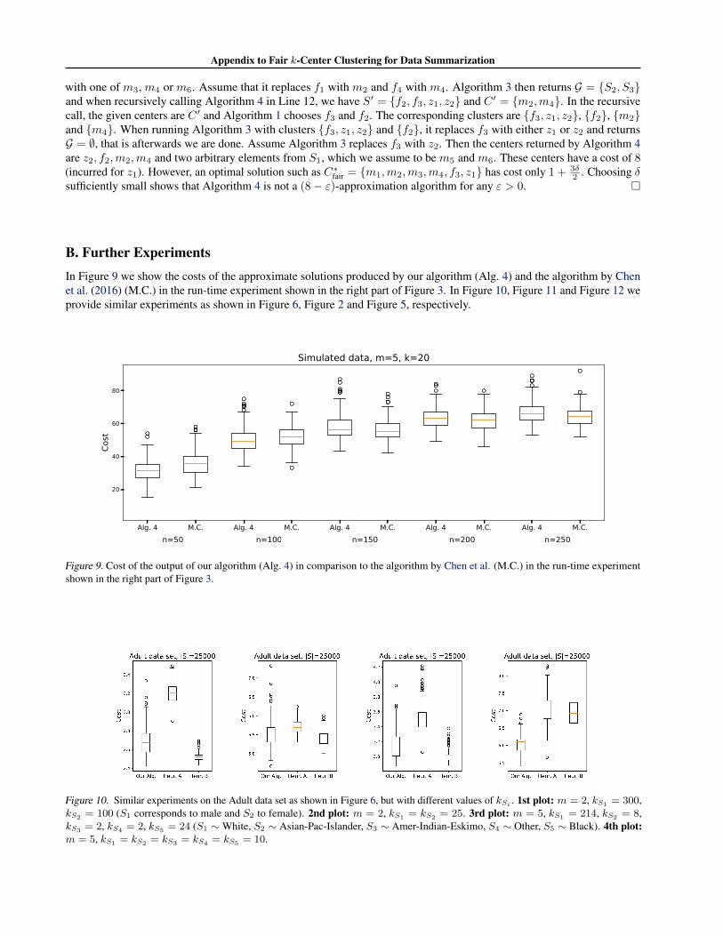
B. Further ExperimentsIn Figure 9 we show the costs of the approximate solutions produced by our algorithm (Alg. 4) and the algorithm by Chenet al. (2016) (M.C.) in the run-time experiment shown in the right part of Figure 3. In Figure 10, Figure 11 and Figure 12 weprovide similar experiments as shown in Figure 6, Figure 2 and Figure 5, respectively.

Figure 9. Cost of the output of our algorithm (Alg. 4) in comparison to the algorithm by Chen et al. (M.C.) in the run-time experimentshown in the right part of Figure 3.

Figure 10. Similar experiments on the Adult data set as shown in Figure 6, but with different values of kSi . 1st plot: m = 2, kS1 = 300,kS2 = 100 (S1 corresponds to male and S2 to female). 2nd plot: m = 2, kS1 = kS2 = 25. 3rd plot: m = 5, kS1 = 214, kS2 = 8,kS3 = 2, kS4 = 2, kS5 = 24 (S1 ∼White, S2 ∼ Asian-Pac-Islander, S3 ∼ Amer-Indian-Eskimo, S4 ∼ Other, S5 ∼ Black). 4th plot:m = 5, kS1 = kS2 = kS3 = kS4 = kS5 = 10.


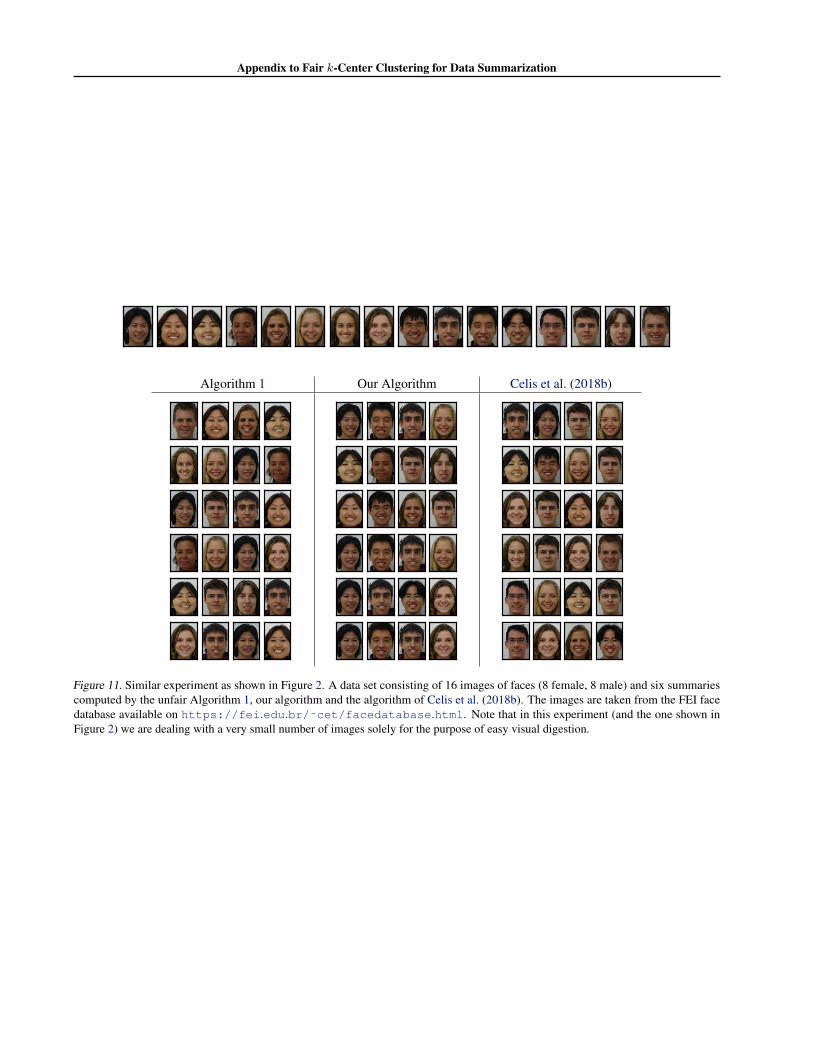
Algorithm 1 Our Algorithm Celis et al. (2018b)

Figure 11. Similar experiment as shown in Figure 2. A data set consisting of 16 images of faces (8 female, 8 male) and six summariescomputed by the unfair Algorithm 1, our algorithm and the algorithm of Celis et al. (2018b). The images are taken from the FEI facedatabase available on https://fei.edu.br/˜cet/facedatabase.html. Note that in this experiment (and the one shown inFigure 2) we are dealing with a very small number of images solely for the purpose of easy visual digestion.

https://fei.edu.br/~cet/facedatabase.html


Figure 12. Similar experiments on the Adult data set as shown in Figure 5, but with different values of kSi . Top left: m = 2, kS1 = 300,kS2 = 100 (S1 corresponds to male and S2 to female). Top right: m = 2, kS1 = kS2 = 25. Bottom left: m = 5, kS1 = 214,kS2 = 8, kS3 = 2, kS4 = 2, kS5 = 24 (S1 ∼White, S2 ∼ Asian-Pac-Islander, S3 ∼ Amer-Indian-Eskimo, S4 ∼ Other, S5 ∼ Black).Bottom right: m = 5, kS1 = kS2 = kS3 = kS4 = kS5 = 10.

Documents

Fair k-Center Clustering for Data Summarization