Failure Prediction of Honeycomb Panel Joints using Finite

Element Analysis

Andrew L. Lyford

Thesis submitted to the Faculty of the

Virginia Polytechnic Institute and State University

In partial fulfillment of the requirements for the degree of

Master of Science

in

Aerospace Engineering

Rakesh K. Kapania

Mayuresh J. Patil

Gary D. Seidel

February 3, 2017

Blacksburg, Virginia

Keywords: Adhesive, Honeycomb, Joint, Finite Element Analysis

Copyright © 2017 by Orbital ATK

Failure Prediction of Honeycomb Panel Joints using Finite

Element Analysis

Andrew L. Lyford

ABSTRACT

Spacecraft structures rely on honeycomb panels to provide a light weight means to support the

vehicle. Honeycomb panels can carry significant load but are most vulnerable to structural

failure at their joints where panels connect. This research shows that predicting sandwich panel

joint capability using finite element analysis (FEA) is possible. This allows for the potential

elimination of coupon testing early in a spacecraft design program to determine joint capability.

Linear finite element analysis (FEA) in NX Nastran was used to show that adhesive failure can

be predicted with reasonable accuracy by including a fillet model on the edge of the fitting.

Predicting the ultimate failure of a joint using linear FEA requires that engineering judgment be

used to determine whether failure of certain bonds in a fitting will lead to ultimate joint failure or

if other bonds will continue to carry the joint’s load.

The linear FEA model is also able to predict when the initiation of core failure will begin. This

has the limitation that the joint will still be able to continue to carry significantly more load prior

to joint ultimate failure even after the core has begun to buckle. A nonlinear analysis is

performed using modified Riks’ method in Abaqus FEA to show that this failure mode is

predictable. The modified Riks’ analysis showed that nonlinear post-buckling analysis of a

honeycomb coupon can predict ultimate core failure with good accuracy. This solution requires

a very high quality mesh in order to continue to run after buckling has begun and requires

imperfections based on linear buckling mode shapes and thickness tolerance on the honeycomb

core to be applied.

Failure Prediction of Honeycomb Panel Joints using Finite

Element Analysis

Andrew L. Lyford

GENERAL AUDIENCE ABSTRACT

Spacecraft structures rely on honeycomb panels to provide a light weight means to support the

vehicle. Honeycomb panels consist of two thin metal sheets separated by a light weight

honeycomb grid. The panels operate in a similar way to how an I-Beam works on a bridge.

These panels can carry significant load but are susceptible to failure because the panels must be

glued together when they are built.

This research shows that predicting honeycomb panel joint capability using finite element

analysis (FEA) is possible. FEA allows the engineer to model and predict failure in complex

structures by mathematically combining many small shapes called elements which have known

behaviors and properties into the shape of the actual tested article. The elements deflect in a

known manner based on the load applied to the model. The honeycomb panel joint is predicted

to break when the deflection in a particular element is higher than the element’s material

capability. Obtaining the load where the panel breaks is critical information to have during the

design of a spacecraft structure.

Using the techniques presented in this thesis allows for the potential elimination of coupon

testing early in a spacecraft design program to determine joint capability. Coupon testing is

where honeycomb panels are built and tested to failure. This testing is very expensive in terms

of both cost and program schedule and therefore using analysis to eliminate its need or to reduce

its scope provides significant benefit to the spacecraft program.

iv

Table of Contents

1 Introduction ................................................................................................................ 1

1.1 Honeycomb Panels in Spacecraft Design......................................................................... 1

1.2 Adhesive Capability Analysis .......................................................................................... 4

1.3 Core Capability Prediction ............................................................................................... 6

2 Honeycomb Panel Joint Adhesive Analysis ........................................................... 10

2.1 Description of Joints Analyzed for Adhesive Failure .................................................... 10

2.1.1 Description of Cup Joint ..................................................................................................... 10

2.1.2 Description of H-Clip Joint ................................................................................................. 14

2.2 Description of Analysis Methods ................................................................................... 17

2.2.1 Description of Method 1 ..................................................................................................... 18

2.2.2 Description of Method 2 ..................................................................................................... 19

2.2.3 Description of Method 3 ..................................................................................................... 24

2.3 Adhesive Analysis Results ............................................................................................. 26

2.3.1 H-Clip Analysis Results ...................................................................................................... 26

2.3.2 Cup Analysis Results .......................................................................................................... 28

2.3.3 Discussion of Results .......................................................................................................... 34

3 Honeycomb Core Failure Prediction ...................................................................... 35

3.1 Unit Cell Analysis .......................................................................................................... 35

3.2 Bushing Analysis............................................................................................................ 39

3.3 Discussion of Core Capability Analysis Results ............................................................ 52

4 Conclusions ............................................................................................................... 53

4.1 Overview and Conclusions............................................................................................. 53

4.2 Future Work ................................................................................................................... 54

v

Bibliography ..................................................................................................................... 56

Appendix A: Element Usage Details .............................................................................. 61

A.1 NX Nastran Model Elements ............................................................................................. 61

A.2 Abaqus FEA Model Elements ........................................................................................... 63

vi

List of Tables

Table 2-1: Summary of the Three Methods Compared ................................................................ 18

Table 2-2: Correlation Factor for each H-Clip Model Mesh Size ................................................ 23

Table 2-3: H-Clip Pull-off Failure Load Predictions compared to Coupon Test Data ................. 28

Table 2-4: Cup Normal Load Failure compared to Coupon Test Data......................................... 33

vii

List of Figures

Figure 1-1: Basic Configuration of Honeycomb Sandwich Panel .................................................. 2

Figure 1-2: Example of Spacecraft Honeycomb Panel Joints ........................................................ 2

Figure 1-3: Example of a Single Lap Joint ..................................................................................... 5

Figure 1-4: Top View of Honeycomb Core with Ribbon Direction Identified .............................. 7

Figure 1-5: Honeycomb Panel showing the Shear Buckling Failure Mode ................................... 8

Figure 2-1: CAD Image of Cup on Honeycomb Panel with Locations of Bonds Identified ........ 11

Figure 2-2: Cup Fitting Coupon .................................................................................................... 11

Figure 2-3: Nominal Cup Coupon Finite Element Model with Critical Items Identified ............. 12

Figure 2-4: Detailed View of Cup showing Adhesive Fillet ........................................................ 12

Figure 2-5: Setup for Cup Coupon Testing................................................................................... 13

Figure 2-6: Load versus Displacement Curves from Cup Normal Load Coupon Tests ............... 13

Figure 2-7: Cup Coupon Failure Mode ......................................................................................... 14

Figure 2-8: CAD Image of H-Clip on Honeycomb Panel with Locations of Bonds Identified ... 15

Figure 2-9: Nominal H-Clip Coupon Finite Element Model with Critical Items Identified ........ 16

Figure 2-10: H-Clip Pull Test Setup ............................................................................................. 16

Figure 2-11: Load versus Displacement Curves from Failure Testing of H-Clip Coupons in Pull-

off Direction .................................................................................................................................. 17

Figure 2-12: H-Clip Adhesive Failure Mode ................................................................................ 17

Figure 2-13: Flow Chart for Method 2 Analysis .......................................................................... 20

viii

Figure 2-14: H-Clip Coupon Model with Varying Mesh Densities (Fine and Coarse Mesh

Models Shown as Symmetric about XZ-Plane) ............................................................................ 21

Figure 2-15: ASTM D1002 Test Specimen Model....................................................................... 21

Figure 2-16: Bending of ASTM D1002 Model under Tensile Load is Excessive Compared to

Coupon .......................................................................................................................................... 22

Figure 2-17: ASTM D5656 Test Specimen Model (Symmetric about XZ-Plane) ....................... 23

Figure 2-18: Bending of ASTM D5656 Model under Tensile Load ............................................ 23

Figure 2-19: ASTM D638 Test Specimen Model......................................................................... 24

Figure 2-20: Quarter-View Model showing Springs used for Method 3 Analysis on Cup .......... 25

Figure 2-21: XZ Symmetric Model of H-Clip showing Springs used for Method 3 Analysis ..... 25

Figure 2-22: Deflection of H-Clip under +X Direction Loading .................................................. 26

Figure 2-23: Shear Stress in Both Adhesive Bonds due to +X Load ........................................... 27

Figure 2-24: Shear Stress in Upper Adhesive Bond due to +X Load ........................................... 27

Figure 2-25: Deflection of Cup due to Unit Pulloff Load (Units in inches) ................................. 29

Figure 2-26: Contour of Normal Stress in Lower Bond due to Unit Load in Pulloff Direction ... 30

Figure 2-27: Contour of Core Shear Adjacent to the Cup ............................................................ 31

Figure 2-28: Catastrophic Failure occurred in Upper Bond of all Coupons ................................. 31

Figure 2-29: Load versus Displacement Curves for Coupons versus Linear Analysis ................ 33

Figure 3-1: Unit Cell Finite Element Model for Abaqus FEA Demonstration............................. 35

ix

Figure 3-2: Summary of Arc Length Method ............................................................................... 36

Figure 3-3: Aluminum 5056-H39 Stress vs. Strain Data Used for Nonlinear Analysis ............... 37

Figure 3-4: Unit Cell Model with Boundary Conditions and Load Applied (Boundary Conditions

Only Shown on Select Nodes along each edge for visual clarity) ................................................ 38

Figure 3-5: Various Steps of Shear Buckling Process for Unit Cell............................................. 39

Figure 3-6: Derived Stress vs. Strain Curve based on Load vs. Displacement Output from Unit

Cell Model .................................................................................................................................... 39

Figure 3-7: Images of Top and Bottom of Bushing Coupon ........................................................ 40

Figure 3-8: Post-Test Image of Bushing Tested in Normal Direction .......................................... 41

Figure 3-9: Load vs. Displacement Curves for Bushings Tested with Force Normal to Panel .... 41

Figure 3-10: Bushing Coupon Finite Element Model with Honeycomb Core Represented at Solid

Brick Elements .............................................................................................................................. 42

Figure 3-11: Bushing Coupon Finite Element Model with Honeycomb Core Represented as

Explicitly Modeled Shell Elements .............................................................................................. 43

Figure 3-12: Half-Section View of Bushing with Honeycomb Core explicitly modeled

identifying Mode Details of Core Thickness ................................................................................ 43

Figure 3-13: Images showing Sample Buckling Mode Shapes of the Coupon’s Honeycomb Core

....................................................................................................................................................... 44

Figure 3-14: Original Mesh of Explicitly Modeled Honeycomb Core where Core was Not

Modeled Symmetric across the YZ-plane at the Center of the Bushing ....................................... 45

x

Figure 3-15: Updated Mesh of Explicitly Modeled Honeycomb Core where Core was Meshed

Symmetric across the Bushing’s Center YZ-Plane ....................................................................... 45

Figure 3-16: Bushing Coupon Test Data Compared against the Analytical Prediction from the

Coupon Model with Honeycomb Core Modeled Explicitly ......................................................... 46

Figure 3-17: Image Showing Deflection and von Mises Stress of Bushing Coupon when

Honeycomb Core Shear Buckling of Core was not triggered....................................................... 47

Figure 3-18: Image Showing Location where Mesh had Two Pieces Bonded together which does

not represent the as-built Bushing Coupon well ........................................................................... 48

Figure 3-19: Comparison of Coupon Test Data to Analytical Prediction when the Washer on the

Top of the Bushing is disconnected from the main spool ............................................................. 48

Figure 3-20: Image Showing Buckling Occurring in the Incomplete Cells around the Fitting .... 49

Figure 3-21: Image showing randomly Distributed Honeycomb Core Thickness Properties across

the coupon (Colors Represent Different Properties) ..................................................................... 50

Figure 3-22: Comparison of Coupon Test Data to Analytical Prediction when the Thickness of

the Honeycomb Core is Altered Randomly and the Core Nodal Positions are Modified ............ 51

Figure 3-23: Comparison of Coupon Test Data to Analytical Prediction of Several Versions of

the Explicit Honeycomb Model .................................................................................................... 51

Figure 3-24: Image Showing Buckled Honeycomb Core around Fitting ..................................... 52

1

1 Introduction

The background for the analysis presented in this work is provided in this chapter. The rationale

for the use of honeycomb panels in spacecraft design and the drawbacks that this design decision

brings are discussed. Additionally, failure modes of honeycomb panels are discussed along with

an introduction to the analytical techniques used to predict both the failure mode type and the

capability of the panel.

1.1 Honeycomb Panels in Spacecraft Design

The need to minimize the mass of a spacecraft structure remains a mainstay requirement for

space vehicle design despite significant advances in launch vehicle capability because of the

inverse relationship between structural mass and the amount of payload that can be carried into

orbit. It is because of this relationship that honeycomb panels are used in nearly every spacecraft

structure designed today. Honeycomb sandwich panels provide a cost-effective means of

providing excellent stiffness to the spacecraft structure with a small mass penalty.

Honeycomb panels are more generally known as sandwich structures because they consist of two

thin skins made of stiff material adhesively bonded to a cellular core as shown in Figure 1-1.

The skins will be described as “facesheets” throughout this document. Moving the stiff

facesheets away from the neutral axis of the plate by means of the lightweight core allows the

designer to increase the second moment of area of the panel significantly with little mass

increase because the second moment increases as a square of the distance of the thin sheet from

the neutral axis.

2

Figure 1-1: Basic Configuration of Honeycomb Sandwich Panel

The benefits of honeycomb panels are clear in that they provide an easily producible,

lightweight, stiff plate-like structure, however drawbacks to their use include the difficulty in

joining them together to form a usable spacecraft structure. The connections between these

panels will be called “joints” throughout this document and an example of a joint is shown in

Figure 1-2.

Figure 1-2: Example of Spacecraft Honeycomb Panel Joints

3

The most likely location of failure in a honeycomb spacecraft structure is in the joints because

the load that are well spread out across the panel get concentrated at these discrete points to be

transmitted to the adjacent panel. The simplest method to minimize the load concentration at

each joint is to increase the quantity of joints between two panels. Joint mass can increase rather

rapidly however because relatively thick metals and dense materials such as steel bolts are often

required for these joints. The joint types discussed in this thesis involve machined fittings that

are either bonded to the edge or in the middle of a honeycomb panel and are bolted to another

fitting bonded to the adjacent panel as can be seen in Figure 1-2.

The most desirable technique for minimizing the quantity of joints and thus the accumulated

joint mass on a spacecraft is to have a robust methodology for predicting a joint’s capability.

This allows the engineer to confidently use a minimal number of joints without having to assign

large uncertainty factors on the joint’s strength capabilities.

The current best method for determining this joint capability is to build and test multiple coupons

to failure in all critical directions. This procedure is often not practical for design of a spacecraft

structure however because the building and testing of coupons requires substantial cost and time.

Coupon tests are therefore best used as a verification test after the spacecraft structural design is

complete. The most economical approach for both schedule and cost for joint capability

predictions for complex joints is the use of the finite element analysis (FEA) method.

With the availability of high-speed computers and robust commercial finite element software, the

FEA allows an engineer to create computational models to predict the capability of joints easily

and relatively quickly. Caution however must be used, as will be demonstrated in this thesis,

because the FEA can predict failure modes in both the adhesive and the panel itself that could be

4

an artifact of numerical limitations of the modeling or because the joint will continue to carry

significant load even after a part of it has failed. This thesis will first discuss the common failure

modes of honeycomb joints and then provide several examples showing FEA’s capability and

limitations for determining joint capability.

1.2 Adhesive Capability Analysis

Adhesives are often implemented in honeycomb panel joints due to their low cost and mass. The

failure modes of bonded joints are generally classified as adhesive failures, cohesive failures or

interlaminar failures [1]. Adhesive failure is a failure mode that occurs between the adhesive and

the substrate. This occurs when the adhesive separates from either the panel or the fitting.

Adhesive failure is sensitive to quality surface preparation prior to implementing the bond

between the fitting and the panel. Cohesive failure is a failure mode within the adhesive layer

itself. There are industry standard test methods to define the cohesive and adhesive bond

strength for adherents which will be discussed in the results chapter. Interlaminar failures only

occur in panels with multi-ply facesheets. This failure mode is not discussed in this document as

all coupon facesheets are made of aluminum.

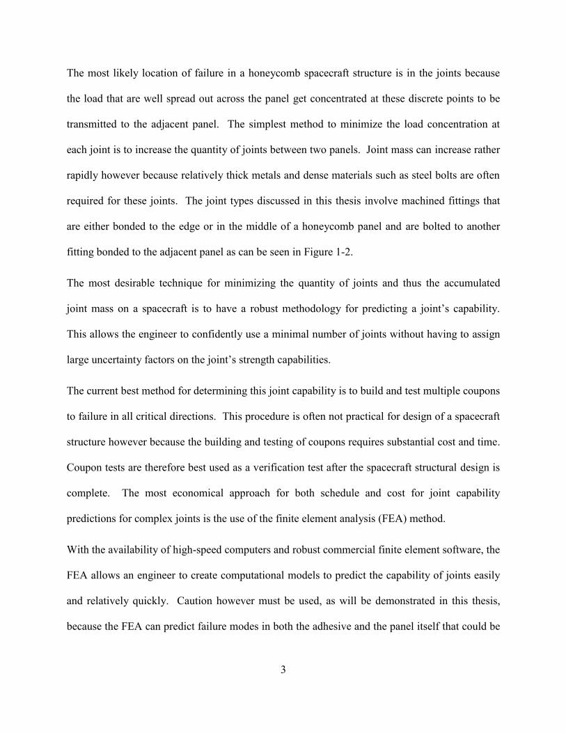
The most traditional and by far the most thoroughly documented joint types are the single lap

joint and double lap joint. A single lap joint is where two bars are bonded together along their

ends as shown in Figure 1-3 and a double lap joint simply add a third bar above the lower bar in

the figure [2-6]. These authors, along with many others, show that adhesive capability in a lap

joint is predictable with reasonable accuracy using hand calculations although some major

constraints were imposed on the adherents. These joint types were verified using FEA by several

authors including Zhu and Kedward who also looked at several variables such as bondline

5

thickness and part alignment and found that uniform bondlines provided the strongest and most

reliable bond [7, 8].

Figure 1-3: Example of a Single Lap Joint

The difficulty of using historical papers for analysis of a bond in a honeycomb panel is that

traditional lap, scarf, and strap joints do not lend themselves well to providing a stiff structure

with minimal mass mainly due to geometrical constraints. Therefore custom joints are generally

designed based on the expected load conditions and the geometry of the panels. The custom

joints often create non-determinant load paths that drive FEA to be the only practical method for

determining joint capability analytically.

Using linear FEA to predict load capability creates several problems due to the adhesive

singularity that is created due to an analytical singularity that is created at the interface between

the soft adhesive and the stiff adherents [9-12]. This singularity can cause the shear stress at the

edge of the adhesive bond to go to infinity as mesh size is decreased. Some authors recommend

using geometric nonlinear effects to mitigate the singularity from the linear analysis [13-14].

This adds significant complexity to the modeling requirements and the analysis time for the

solver to provide results and is therefore not desirable. It has been shown that if a fillet is

modeled coming off of the edge of the adhesive which does exist in practice, then this singularity

6

is reduced and results will show good correlation to hand calculations and test data for lap joints

[15-18].

Metallic fittings bonded to the sandwich honeycomb panel provide a means to spread a point

load out over a relatively wide area. This allows for the use of a traditional fastener to hold two

panels together through their bonded fittings. The fittings can also be bonded together but this

adds significant complexity to the design and prevents the panels from being taken apart if

desired in the future. As noted by Devadas, Sunikumar and Sajeeb [19], there is limited research

available discussing bonded joints on honeycomb panels. These authors investigated a butt joint

between two honeycomb panels and showed that varying the fitting, facesheet, and honeycomb

core thickness can greatly affect the strength of the joint. Additionally, Lundgren, Smeltzer and

Kapania investigated the capability of several honeycomb panel double strap joint designs [12].

These authors used plane strain linear FEA with a fillet modeled on the adhesive to predict the

stress in the double strap joint. They also investigated the effect of various parameters such as

bondline thickness and the effect of defects in the bond [12].

This thesis will show in chapter 2 that bonding honeycomb panels together through fittings is a

practical method for spacecraft design and that the failure loads are predictable compared to test

data.

1.3 Core Capability Prediction

The other major failure other than bond failure for a honeycomb joint is the core itself failing.

The core, as discussed previously is a low density material that has the primary function of

keeping the facesheets apart so that the panels will carry higher bending loads. The core

7

presented in the examples in this thesis is honeycomb core, but other materials such as foam can

also be used [20, 21].

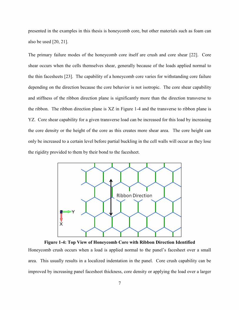
The primary failure modes of the honeycomb core itself are crush and core shear [22]. Core

shear occurs when the cells themselves shear, generally because of the loads applied normal to

the thin facesheets [23]. The capability of a honeycomb core varies for withstanding core failure

depending on the direction because the core behavior is not isotropic. The core shear capability

and stiffness of the ribbon direction plane is significantly more than the direction transverse to

the ribbon. The ribbon direction plane is XZ in Figure 1-4 and the transverse to ribbon plane is

YZ. Core shear capability for a given transverse load can be increased for this load by increasing

the core density or the height of the core as this creates more shear area. The core height can

only be increased to a certain level before partial buckling in the cell walls will occur as they lose

the rigidity provided to them by their bond to the facesheet.

Figure 1-4: Top View of Honeycomb Core with Ribbon Direction Identified

Honeycomb crush occurs when a load is applied normal to the panel’s facesheet over a small

area. This usually results in a localized indentation in the panel. Core crush capability can be

improved by increasing panel facesheet thickness, core density or applying the load over a larger

8

area. The joint must be designed to spread out the load to increase the capability for these failure

modes. Heimbs and Pein discuss several different methods for joining honeycomb panels and

show that FEA can be a good method for predicting core failure [24].

Core shear and core crush are simple to predict with simple analytical calculations or using a

simple finite element model for most loading and geometrical conditions. This thesis will

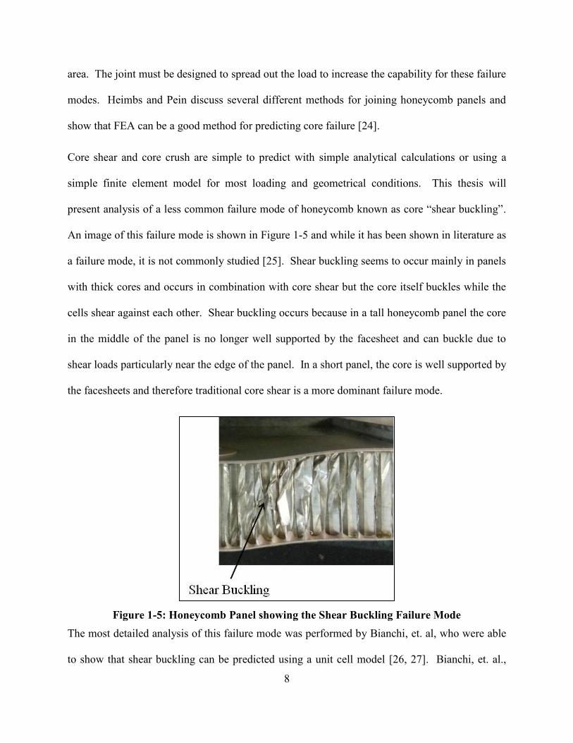
present analysis of a less common failure mode of honeycomb known as core “shear buckling”.

An image of this failure mode is shown in Figure 1-5 and while it has been shown in literature as

a failure mode, it is not commonly studied [25]. Shear buckling seems to occur mainly in panels

with thick cores and occurs in combination with core shear but the core itself buckles while the

cells shear against each other. Shear buckling occurs because in a tall honeycomb panel the core

in the middle of the panel is no longer well supported by the facesheet and can buckle due to

shear loads particularly near the edge of the panel. In a short panel, the core is well supported by

the facesheets and therefore traditional core shear is a more dominant failure mode.

Figure 1-5: Honeycomb Panel showing the Shear Buckling Failure Mode

The most detailed analysis of this failure mode was performed by Bianchi, et. al, who were able

to show that shear buckling can be predicted using a unit cell model [26, 27]. Bianchi, et. al.,

9

tested coupons to failure in the ribbon direction, transverse to ribbon and at an angle of 45° to the

ribbon. They then used Riks’ method to reproduce load versus displacement curve from the test

on a unit cell model. This thesis will demonstrate the use of Abaqus’ modified Riks’ method on

a unit cell to create a core buckling failure and then analyze a detailed coupon model that was

tested and demonstrated to have a core buckling failure. Details on this analysis will be provided

in Section 3.

10

2 Honeycomb Panel Joint Adhesive Analysis

This chapter discusses predicting adhesive failure in a bonded honeycomb joint. The main goal

of the analysis in this thesis is to show that joint analysis on a honeycomb panel is reliable

enough that coupon testing can be delayed until it fits well into the program flow. In other

words, the goal of this analysis is not to show that the prediction is perfect compared to a coupon

test but that it is close enough that the same process could be repeated on other joint designs with

confidence early on in the spacecraft design cycle. The analysis on the adhesive was performed

with linear FEA so that the analysis run times are low and the models are relatively easy to build

[28, 29]. This chapter will show that the analytical predictions for joint capability are similar to

coupon test predictions when the process is followed.

2.1 Description of Joints Analyzed for Adhesive Failure

Two specific types of joints are discussed in this chapter, a “cup” and an “H-Clip”. This section

provides details about each type of joint and describes the models that were created for each

joint.

2.1.1 Description of Cup Joint

A CAD image of the cup on the honeycomb panel is shown in Figure 2-1 with the bond locations

identified. The cup was tested to failure with six coupons, one of which is shown in Figure 2-2.

The cup is bonded into a panel with aluminum facesheets and aluminum honeycomb core in a

pre-drilled hole that is narrow on the lower facesheet and wide on the upper facesheet to

accommodate the geometry of the cup. The lower bondline between the cup and the lower

facesheet is located inside of the panel and the upper bondline is located on the outside of the

upper facesheet.

11

Figure 2-1: CAD Image of Cup on Honeycomb Panel with Locations of Bonds Identified

Figure 2-2: Cup Fitting Coupon

Figure 2-3 shows the finite element model created to predict failure of the cup coupon with

critical items identified. The model has 80,000 nodes and 75,000 elements and is run using the

NX Nastran solver. The cup, adhesive, and honeycomb core are modeled using solid linear

CHEX elements. The facesheet is modeled with CQUAD4 shell elements. A description of

these element types is provided in Appendix A. The core is modeled using a homogenous

anisotropic material that matches manufacturer provided stiffness for the crush direction (X) and

the core shear directions (XY and XZ). All other materials are isotropic including the thin

adhesive bond line. The load is applied and the model is constrained via RBE2 rigid elements

that simulate the rigidity of a preloaded fastener to rigid test equipment at these locations. The

12

load is applied in the +P direction annotated onto Figure 2-3 which corresponds to the –X

direction in the coordinate system shown.

Figure 2-3: Nominal Cup Coupon Finite Element Model with Critical Items Identified

Figure 2-4 shows a more detailed section cut of the cup fitting which identifies important

elements of the adhesive modeling. The adhesive has an extra element past the edge of the bond

to model to decrease the effect of the singularity from the linear FEA caused by the large

stiffness difference between the metallic adherents and the soft adhesive. The results will show

that this is an effective modeling technique and provides representation of the adhesive that spills

out of the bonded area during manufacturing [12].

Figure 2-4: Detailed View of Cup showing Adhesive Fillet

13

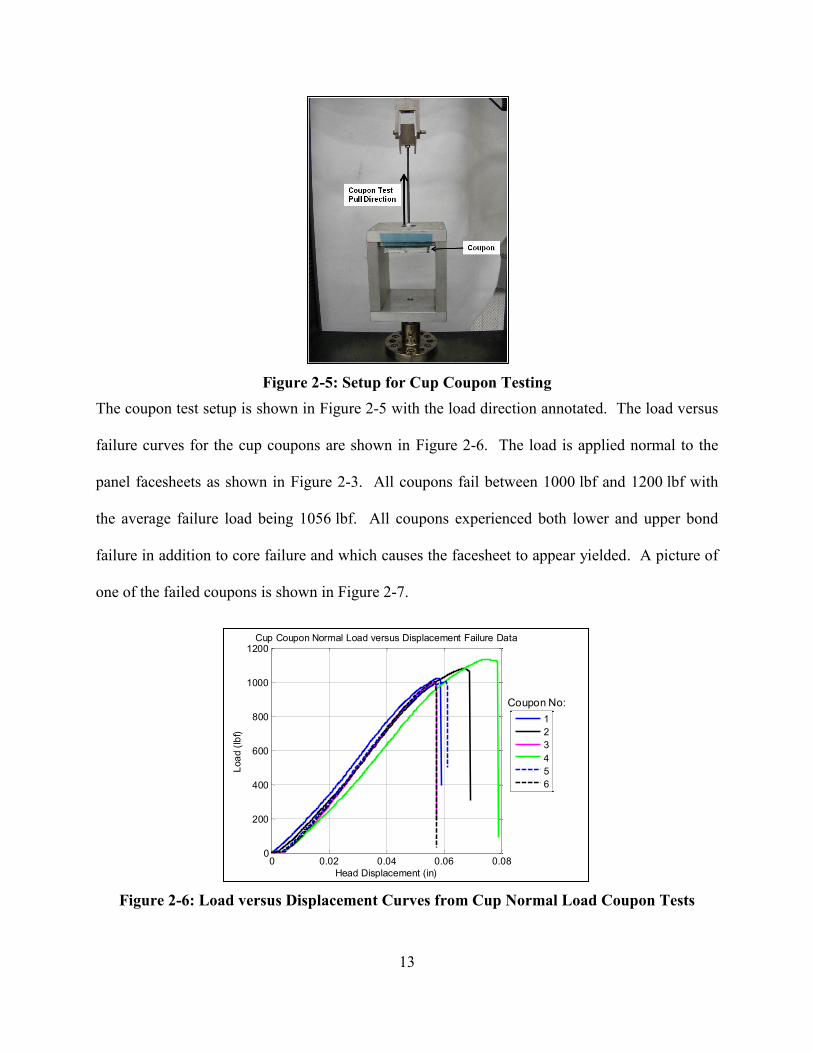
Figure 2-5: Setup for Cup Coupon Testing

The coupon test setup is shown in Figure 2-5 with the load direction annotated. The load versus

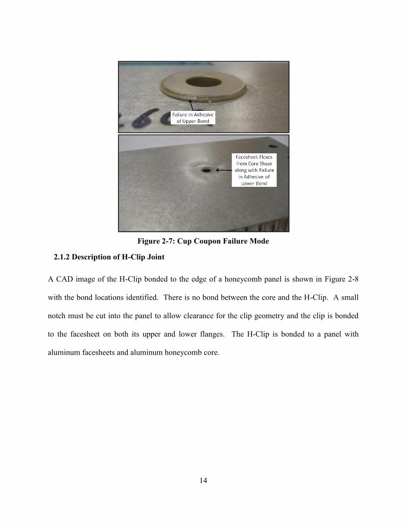
failure curves for the cup coupons are shown in Figure 2-6. The load is applied normal to the

panel facesheets as shown in Figure 2-3. All coupons fail between 1000 lbf and 1200 lbf with

the average failure load being 1056 lbf. All coupons experienced both lower and upper bond

failure in addition to core failure and which causes the facesheet to appear yielded. A picture of

one of the failed coupons is shown in Figure 2-7.

Figure 2-6: Load versus Displacement Curves from Cup Normal Load Coupon Tests

0 0.02 0.04 0.06 0.080

200

400

600

800

1000

1200

Head Displacement (in)

Loa

d (

lbf)

Cup Coupon Normal Load versus Displacement Failure Data

1

2

3

4

5

6

Coupon No:

14

Figure 2-7: Cup Coupon Failure Mode

2.1.2 Description of H-Clip Joint

A CAD image of the H-Clip bonded to the edge of a honeycomb panel is shown in Figure 2-8

with the bond locations identified. There is no bond between the core and the H-Clip. A small

notch must be cut into the panel to allow clearance for the clip geometry and the clip is bonded

to the facesheet on both its upper and lower flanges. The H-Clip is bonded to a panel with

aluminum facesheets and aluminum honeycomb core.

15

Figure 2-8: CAD Image of H-Clip on Honeycomb Panel with Locations of Bonds Identified

Figure 2-9 shows the finite element model of the H-Clip coupon that was created to predict the

clip’s failure mode. It is setup in a similar fashion to the cup and is also solved using NX

Nastran. The facesheet is modeled using CQUAD4 shell elements and the H-Clip, honeycomb

core, and adhesive are modeled using CHEX linear solid elements. The core is modeled using

homogenous anisotropic material properties just as with the cup. Three different H-Clip models

were created to check the sensitivity of the adhesive failure results to mesh size. The coarse

model has 58,000 elements, the medium model has 76,000 elements and the fine model has

160,000 elements.

16

Figure 2-9: Nominal H-Clip Coupon Finite Element Model with Critical Items Identified

Ten H-Clip coupons were tested to failure and the load was applied in the pull-off direction (+X

in Figure 2-9). An image of the test setup is shown in Figure 2-10 and the load versus

displacement curves are shown in Figure 2-11. All of the coupons failed at loads between

2200 lbf and 2900 lbf with an average failure load of 2590 lbf. The failure mode was adhesive

shear and a picture of one of the failed H-Clip coupons is shown in Figure 2-12.

Figure 2-10: H-Clip Pull Test Setup

17

Figure 2-11: Load versus Displacement Curves from Failure Testing of H-Clip Coupons in

Pull-off Direction

Figure 2-12: H-Clip Adhesive Failure Mode

2.2 Description of Analysis Methods

Three adhesive methods were used to analyze the adhesive to determine their effectiveness. The

methods are summarized in Table 2-1 and are detailed further below. The first two methods use

the modeling approaches outlined in Section 2.1 and the third method utilizes springs to model

the adhesive [30].

0 0.02 0.04 0.06 0.080

500

1000

1500

2000

2500

3000

Head Displacement (in)

Loa

d (

lbf)

H-Clip Coupon Pulloff Load versus Displacement Failure Data

1

2

3

4

5

6

7

8

9

10

Coupon No:

18

Table 2-1: Summary of the Three Methods Compared

Method No. Description

1

Build coupon model using 3D solid elements for all components in panel and

the joint with at least 3 elements through the thickness of all parts

o Facesheet may be modeled with shells or solids

Apply load to coupon and determine the load required for each of the

applicable failure loads using linear scaling

Determine which failure modes are local (will not cause total joint failure)

and which are catastrophic (joint will lose load-bearing capability)

Predicted failure load is the force that causes the first catastrophic failure as

judged by the analyst

2

Build the same model as described in Method 1

Build model of the ASTM test setup used to determine adhesive allowable

using the same mesh size for each failure modes (multiple models are

necessary if the mesh size is inconsistent)

Apply load to the ASTM model and compare the maximum stress predicted

by the model compared to the stress expected based on the hand calculation

the ASTM specification uses to calculate the stress at failure

Use calculated factor to scale the adhesive specification allowables and use

procedure from Method 1 to calculate catastrophic failure load with updated

allowables

3

Build the same finite element model as in Method 1 but replace solid element

in adhesive with springs with tuned stiffness [30]

Apply load to the model and convert the shear and normal forces in the

adhesive springs to shear and tensile/compressive stress by dividing by the

area each spring represents

Compare stress in the adhesive and other components in the joint to the

appropriate allowables to calculate the failure load

2.2.1 Description of Method 1

Method 1 requires the joint coupon finite element model to be created with all significant

features modeled. The honeycomb core, fitting and adhesive must be modeled with brick

element with a minimum of three elements through the thickness to capture local stress fields.

The facesheet may be modeled with either brick or shell elements of the appropriate thickness

but shell elements reduce the total model size significantly. The adhesive is modeled using the

nominal thickness for the joint unless the structure has already been built in which case the as-

built thickness would be included in the model.

The loads are applied to the model with the coupon’s boundary conditions set to match the

coupon test and the stress is recovered throughout the model. Each potential failure mode for the

19

joint is assessed and its applicable failure mode is calculated. The analyst must determine

whether the failure mode would simply be a local failure within the joint or whether the failure

of the component would lead to catastrophic failure of the joint. The final failure load is the

minimum load for a catastrophic failure as determined by the analyst.

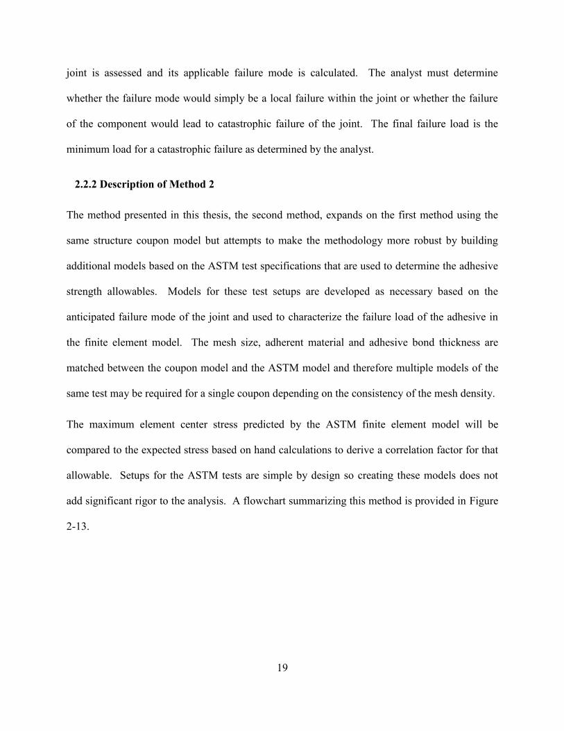
2.2.2 Description of Method 2

The method presented in this thesis, the second method, expands on the first method using the

same structure coupon model but attempts to make the methodology more robust by building

additional models based on the ASTM test specifications that are used to determine the adhesive

strength allowables. Models for these test setups are developed as necessary based on the

anticipated failure mode of the joint and used to characterize the failure load of the adhesive in

the finite element model. The mesh size, adherent material and adhesive bond thickness are

matched between the coupon model and the ASTM model and therefore multiple models of the

same test may be required for a single coupon depending on the consistency of the mesh density.

The maximum element center stress predicted by the ASTM finite element model will be

compared to the expected stress based on hand calculations to derive a correlation factor for that

allowable. Setups for the ASTM tests are simple by design so creating these models does not

add significant rigor to the analysis. A flowchart summarizing this method is provided in Figure

2-13.

20

Figure 2-13: Flow Chart for Method 2 Analysis

The failure mode for the cup coupons is a tensile failure and the failure mode for the H-Clip

coupon is in shear. The shear failure stress provided by the manufacturer of the adhesive is

developed from the ASTM lap shear test. Models of this test were created for the three mesh

sizes used in the H-Clip coupon finite element models shown in Figure 2-14 to assess how much

the finite element model was over-predicting the stress due to the singularity compared to a hand

calculation assuming the shear will be constant across the bond.

A sample model of the ASTM D1002 test is shown in Figure 2-15. It was found that the peak

stress in the bond was predicted to be between 68% and 86% above the expected stress for a joint

with constant shear depending on the mesh size of the model. However, as shown in Figure

2-16, the adherents are very thin strips that bend due to the offset tensile load will therefore put

high peel loads at the ends of the adhesive which invalidates the constant shear assumption. The

Create Joint

Global Model

(try to keep mesh

size uniform in

critical locations)

Identify mesh size

– can be multiple

sizes if necessary

Create global model of adhesive

test setup that was used to derive

allowable (tensile, shear, peel as

applicable) – Mesh must be same

size as Joint Global Model

Apply loads to global

model

Apply loads to

global specification

models

Determine FEM

Allowables by

comparing stress

in local FEM to

test stress

Use FEM

Allowables from

Spec Models to

determine failure

load of joint

Repeat for another

mesh size to

determine if

method converges

START

END if mesh

converges

21

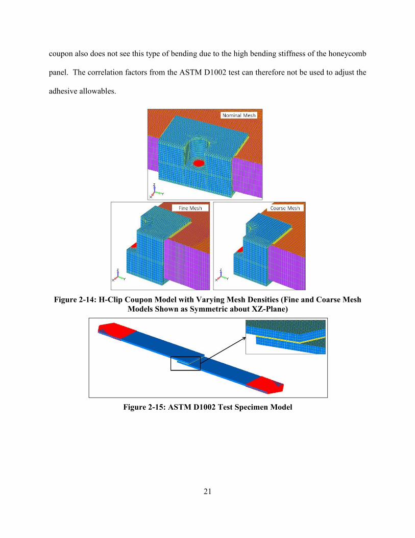
coupon also does not see this type of bending due to the high bending stiffness of the honeycomb

panel. The correlation factors from the ASTM D1002 test can therefore not be used to adjust the

adhesive allowables.

Figure 2-14: H-Clip Coupon Model with Varying Mesh Densities (Fine and Coarse Mesh

Models Shown as Symmetric about XZ-Plane)

Figure 2-15: ASTM D1002 Test Specimen Model

22

Figure 2-16: Bending of ASTM D1002 Model under Tensile Load is Excessive Compared to

Coupon

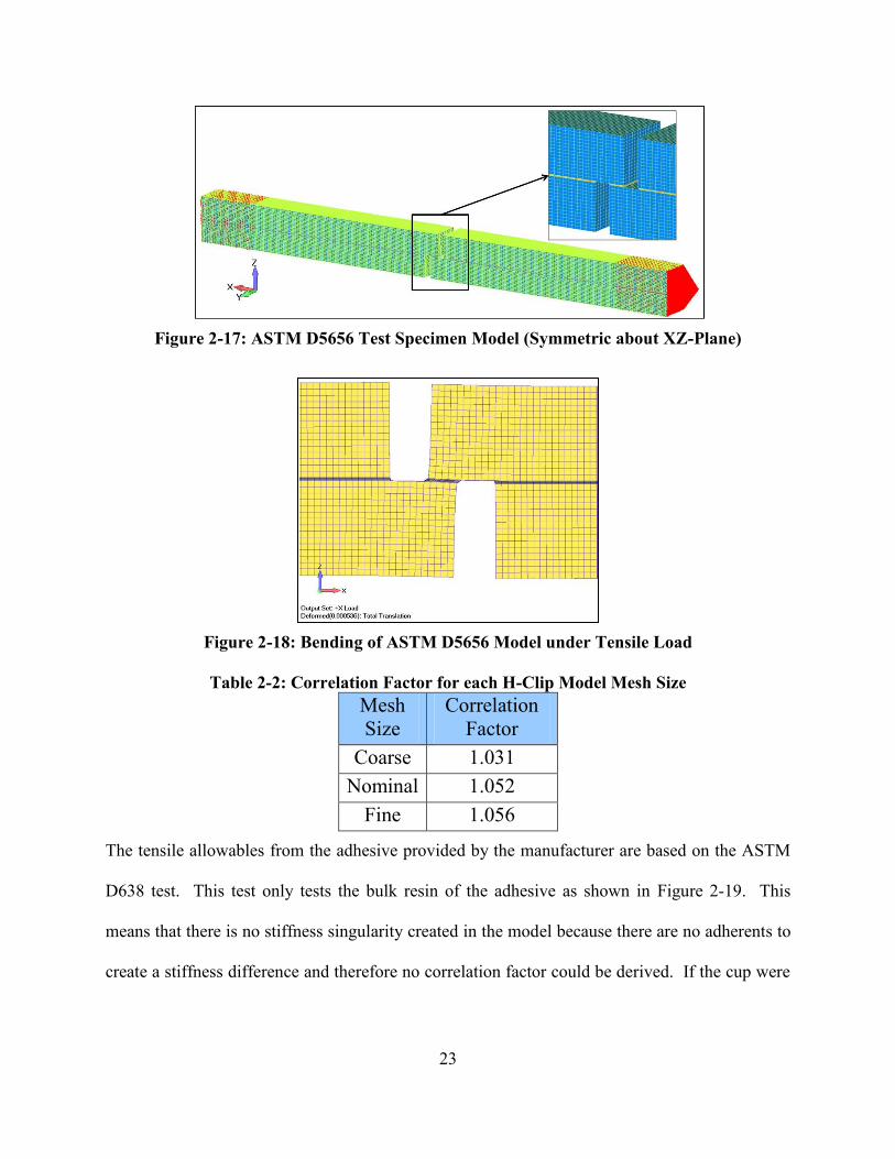
ASTM has established a test with thick adherents to minimize the peel loads of the adhesive in

ASTM D5656. Models of this test setup were created for each mesh size and one of the models

is shown in Figure 2-17. The specimen consists of two thick beams bonded to each other with

two notches cutout in the middle to isolate a thin strip of adhesive where the failure stress is

determined. The displacement shows that the adhesive has very near constant shear across its

length as shown in Figure 2-18. The correlation factors derived for this model are given in Table

2-2 for each mesh size. They provide very little modification to the results but the overall factor

is higher for the smaller mesh as expected for a model with a singularity that will not converge.

These correlation factors are applied to the lap shear allowable provided by the manufacturer

based on the D1002 test because this is the only strength allowable available and it is

conservative to do so based on the shear stress results of the D1002 lap shear models.

23

Figure 2-17: ASTM D5656 Test Specimen Model (Symmetric about XZ-Plane)

Figure 2-18: Bending of ASTM D5656 Model under Tensile Load

Table 2-2: Correlation Factor for each H-Clip Model Mesh Size

Mesh

Size

Correlation

Factor

Coarse 1.031

Nominal 1.052

Fine 1.056

The tensile allowables from the adhesive provided by the manufacturer are based on the ASTM

D638 test. This test only tests the bulk resin of the adhesive as shown in Figure 2-19. This

means that there is no stiffness singularity created in the model because there are no adherents to

create a stiffness difference and therefore no correlation factor could be derived. If the cup were

24

failing in peel, models could have been created of the D1876 test could have been created to

derive a correlation factor but the cup failure is due to tensile stress in the middle of the bond.

Figure 2-19: ASTM D638 Test Specimen Model

2.2.3 Description of Method 3

The third method uses tuned springs based on the stiffness derived by Loss and Kedward [30].

The authors presented the method as a means to model double and single lap joints. This

analysis will assess whether it is a viable method for analyzing more complicated geometry and

loading conditions.

This method uses the same model as Method 1 but the brick elements modeling the adhesive are

replaced by spring elements with shear and normal stiffness calculated based on formulas

presented in [30]. These formulas provide different stiffness values in both shear and tensile for

elements in the middle of the bond, along the edge and on the corners based on the volume of

adhesive that element represents. The stiffness of the springs is a function of the adhesive

material properties, the adhesive bond thickness and the mesh size. There is no rotational

stiffness applied to the springs.

Figure 2-20 shows a quarter-symmetric model of the cup fitting with tuned springs modeling the

adhesive. A different spring stiffness value is used at each radial station to take into account the

25

change in bond area represented by each spring. Figure 2-21 shows the nominal mesh H-Clip

model with the internal, edge and corner springs identified. This method is desirable because the

spring elements are computationally inexpensive compared to the brick elements and the results

are simple to post-process and interpret. The shear stress is calculated by dividing the total shear

force recovered in each of the springs by the element area that the spring represents [30]. Tensile

stress is calculated by dividing the normal force recovered in each of the springs by the element

area that each spring represents [30].

Figure 2-20: Quarter-View Model showing Springs used for Method 3 Analysis on Cup

Figure 2-21: XZ Symmetric Model of H-Clip showing Springs used for Method 3 Analysis

26

2.3 Adhesive Analysis Results

2.3.1 H-Clip Analysis Results

The joints were analyzed using each of the methodologies described in Section 2.2 where

applicable. A sample deflection of the H-Clip model under a default load that was scaled to find

the failure load is shown in Figure 2-22. The load is transmitted from the bolt and because the

fastener is on the –Z side of the clip, more of the load is transmitted into the lower bond than the

upper bond.

Figure 2-22: Deflection of H-Clip under +X Direction Loading

The maximum shear stress for this default load on the nominal mesh model is shown in Figure

2-23 for both bonds. The peak shear stress occurs in the lower bond at the outside perimeter of

the H-Clip on the edge of the panel. The peak stress in the upper bond is about 60% of the peak

stress in the lower bond and this contour is shown in Figure 2-24. The peak shear stress in the

upper bond occurs in the center of the bond closest to where the load is transmitted into the

adhesive. Other modes were assessed for failure such as for tensile stress, peel load, facesheet

yield and H-Clip yield by comparing the applicable stress or force to the relevant strength

allowable but adhesive shear stress was found to be the only mode that could cause failure.

27

Figure 2-23: Shear Stress in Both Adhesive Bonds due to +X Load

Figure 2-24: Shear Stress in Upper Adhesive Bond due to +X Load

The predicted failure loads for the upper and lower bonds for each of the three methods are

compared along with the results of the coupon test data in Table 2-3. The computational results

show that the lower bond begins to fail at a load significantly less than the test data. The peak

shear stress in the lower bond however occurs in localized areas as seen in Figure 2-23 that will

not cause final catastrophic failure of the joint where the joint loses load carrying capability.

Therefore using Method 1, the next failure mode must be assessed which is the shear stress in the

upper bond. As shown in Figure 2-24, the maximum shear stress in the upper bond occurs over a

28

large percentage of the bond area. If this large section of adhesive fails, the joint will lose load

carrying capability and therefore this is considered a catastrophic failure.

Table 2-3 shows that the failure loads for the upper bond are predicted very well compared to the

test data for both Method 1 and Method 2. Method 2 scales the failure load from Method 1 by

the correlation factor presented in Table 2-2. These correlation factors were found to be small

for these mesh sizes and thin bondline and therefore the results are effectively the same although

Method 2 has slightly better convergence than Method 1 because the correlation factor for the

finer mesh is larger than for the coarse mesh.

The predicted failure loads predicted using the springs from Method 3 are also shown in Table

2-3. The failure loads for the lower bond are in the general range of the failure in the test data

but the upper bond failure occurs at a significantly higher load than the coupons failed at during

test. Additionally, the convergence of Method 3 was poorer than Methods 1 and 2 with an over

500 lbf difference between the failure load prediction in the lower bond for the coarse and fine

mesh sizes.

Table 2-3: H-Clip Pull-off Failure Load Predictions compared to Coupon Test Data

2.3.2 Cup Analysis Results

The first cup capability analysis used Method 1 from Section 2.2. A unit load was applied in the

coordinate system’s –X direction at the center of the cup in a similar way as the loaded test

Method 1 Method 2 Method 3

Coarse 1697 1751 2576

Nominal 1476 1554 2218

Fine 1382 1460 1926

Coarse 2723 2808 3844

Nominal 2465 2594 3719

Fine 2349 2482 3350

Failure Type

Local

Catastrophic Upper Bond

Lower Bond2590 lbf Average;

Range of 2291 -

2793 lbf

Failure Load Prediction (lbf)Test DataMesh DensityLocation

29

coupon. This element has its master node at the geometrical center of the cup hole which

supports a fastener in the test and makes several rows of nodes in the cup dependent to ensure the

load is transmitted to the coupon in an as-tested fashion.

The predicted deflection shape due to the unit load with the displacement exaggerated is shown

in Figure 2-25. The deformed shape shows that the cup deforms the panel facesheets with tensile

load transmitted through the bond. The failure modes that are tracked are tensile and

compressive stresses in the upper and lower bonds and shear through the core. There is shear

stress in the bond also but it is small compared to the tensile stress. The stress in the facesheet

and cups are small with respect to their allowables as well as the shear stress in the bonds. When

assessing each failure mode, it must be decided whether it would be detrimental to the joint’s

ability to carry load. If the failure mode is not detrimental, other failure modes are assessed as

long as the joint can continue to carry load.

Figure 2-25: Deflection of Cup due to Unit Pulloff Load (Units in inches)

Figure 2-26 shows the normal stresses in the lower bond. The image shows that the applied

force puts a tensile load on the inside of the lower bond which changes to a compression load but

then back to a tensile load at the bond outside edge. This bond is predicted to fail in tension at

30

the outside edge at a load of 340 lbf but because the load can then be transmitted to the top

facesheet this failure mode is not detrimental to the load carrying capability of the joint.

Figure 2-26: Contour of Normal Stress in Lower Bond due to Unit Load in Pulloff

Direction

The next failure mode assessed was shear through the core in the vicinity of the cup fitting. The

core has been removed at the immediate location where the cup is installed but remains adjacent

to the cup and is not attached directly to the cup. The core is responsible for transferring load

between the facesheets by carrying the load in shear. When the shear capability of the core is

exceeded, the cells will plastically deform with respect to each other. The shear stress prediction

within the core is shown in Figure 2-27. The results in the first row of elements along the inside

radius of the core are excluded to avoid artificially high edge stress discontinuities. The core

shear predicts that the cup fitting will start to fail at 820 lbf using typical core strength allowables

from the manufacturer. However, this failure mode is also not detrimental as the core is carrying

the load transmitted from the cup directly from the load application point to the large flange

bonded to the upper facesheet.

31

Figure 2-27: Contour of Core Shear Adjacent to the Cup

Essentially, the lower bond and core failure lead to a redistribution of the load as the coupon

deforms and the force transmitted through the cup continues to load the top adhesive. The

normal stress in the upper bond is displayed in Figure 2-28a. The tensile stress in the upper

bond predicts a failure of 1102 lbf which is similar to the coupon test data which failed at an

average of 1056 lbf in the upper bond as shown in Figure 2-28b.

Figure 2-28: Catastrophic Failure occurred in Upper Bond of all Coupons

Once the upper bond fails, the joint can no longer carry load as seen in the load-deflection curves

from the coupon tests in Figure 2-29. The displacement versus load curve from the model is

overlaid on the coupon testing crosshead displacement curves. The slope indicates the

32

displacement of the model is under-predicted with respect to the test data which is expected as

the material is assumed to be linear elastic as opposed to non-linear plastic and the analysis does

not take into consideration large deformation and the progressive failure of materials. It must

also be noted that the displacement for the test data is measured at the head of the tensometer and

not at the coupon itself meaning that deflection of the load train, which was relatively long as

seen in Figure 2-5, is included in the test data but is not accounted for in the linear model.

The coupon test data shows no indication of a stiffness change in the load-deflection curve due to

the lower bond beginning to fail at 340 lbf, indicating it is inconsequential in the stiffness of the

joint. The slopes of all of the curves do begin to decrease slightly (non-linear behavior)

beginning at about 800 lbf, where the model predicts the core to start failing. This change in

slope indicates the core is beginning to shear or crush locally as the core absorbs and

redistributes the energy from the load.

33

Figure 2-29: Load versus Displacement Curves for Coupons versus Linear Analysis

The failure loads predicted by Method 1 are based upon tensile loading and therefore Method 2

is not applicable because a correlation factor could not be derived for the ASTM D638 test

specimen as outlined in Section 2.2.3.

The results for Method 3 on the cup are very similar to the results from the H-Clip. The failure

of the lower bond is predicted at a force similar to the test data but the overall failure which will

occur in the upper bond is predicted to occur at a load significantly higher than the test data.

Table 2-4 summarizes the failure loads for Methods 1 and 3 compared to the test data.

Table 2-4: Cup Normal Load Failure compared to Coupon Test Data

Failure

Type Location

Failure Load Prediction (lbf)

Test Data Method

1

Method

2

Method

3

Local Lower

Bond 340 N/A 1052 1056 lbf Average;

Range of 1016 lbf

– 1150 lbf Catastrophic Upper

Bond 1102 N/A 6620

34

2.3.3 Discussion of Results

The results from both the cup and H-Clip analysis show that Method 1 is the most reliable

method for predicting the failure load of the joint. This method predicted the failure of the cup

within 5% of the average failure load of the cup coupons and predicted the failure of the H-Clip

within 10% for the worst-case mesh size but within 5% for the two finer mesh sizes. This

method is more computationally expensive than Method 3 because of the large number of brick

elements required to accurately model the bond compared to the springs, but Method 3 proved to

be unable to accurately predict the failure of a complex joint. Method 3 might be ill-suited to

predict failure load for this type of joint because the interactions of the upper and lower bonds in

these joints may disqualify some of the assumptions made in deriving the stiffness of the tuned

springs.

Method 2 proved to be largely ineffective in reducing the singularity created by the interactions

of the adhesive and the adherents in the joint although taking the stress at the center of the

element seems to mitigate this amplification mostly. It was not possible to derive a correlation

factor for tensile stress because there are no adherents in the ASTM D638 test. The correlation

factors derived for the shear stress had to be calculated based upon a thick adherents test from

ASTM D5656 instead of the lap shear test in ASTM D1002 because the lap shear test induces a

peel load in the adhesive because of bending in the thin adherents. This was not desirable

because the strength allowables from the adhesive published by the manufacturer are based upon

ASTM D1002 lap shear testing and the correlation factors derived from the thick adherents test

ranged from between 3% and 6% depending on mesh size which was not enough to offset the

stress differences seen in the H-Clip coupons of varying mesh sizes.

35

3 Honeycomb Core Failure Prediction

This chapter presents analysis that predicts the honeycomb core capability in a joint using high

fidelity nonlinear FEA in the Abaqus FEA solver. The analysis is more complex than the linear

FEA presented in Section 2 but provides an interesting method if capability for the honeycomb

core is desired after it has begun to fail.

3.1 Unit Cell Analysis

The first step in analyzing a complex honeycomb joint is to start with a simple model of a unit

cell to demonstrate the capabilities of Abaqus FEA and understand the process that will be

required for a full coupon model. Figure 3-1 shows the unit cell model that was created which

contains about 2,500 nodes and elements.

Figure 3-1: Unit Cell Finite Element Model for Abaqus FEA Demonstration

Modified Riks’ method was chosen as the solver approach due to its known ability to solve post-

buckling problems such as honeycomb failure. This method is ideally suited for simulations

where the derivative of the load versus displacement changes sign or in other words where the

load carried by the member reduces as it is displaced [31]. The modified Riks’ method in

Abaqus FEA solves for equilibrium using an arc length approach rather than the Newton’s

36

method used in traditional nonlinear analysis. The limitation of Newton’s method for solving for

equilibrium is that it requires a monotonic increase in load or displacement through each iterative

step. In post-buckling analysis, a monotonic load increase is extremely unlikely. The general arc

length solve approach is summarized in Figure 3-2 and shows how it is able to solve for

equilibrium with imposing the monotonic load increase constraint using arc length along the

curve as an additional variable. Modified Riks’ method was successfully used by Bianchi,

Aglietti, and Richardson to prove that shear buckling in a simple panel coupon matched the

buckling of an equivalent unit cell [27].

Figure 3-2: Summary of Arc Length Method

The first step for the analysis is to define material properties for the Aluminum 5056-H39

honeycomb core used in the unit cell. Due to its use almost exclusively as a component of

manufactured honeycomb, there is little data providing explicit strength properties for the

material itself. A yield strength value of 50 ksi and an ultimate strength of 60 ksi were assumed

based on similar materials and other tempers of Aluminum 5056. The stress-strain curve was fit

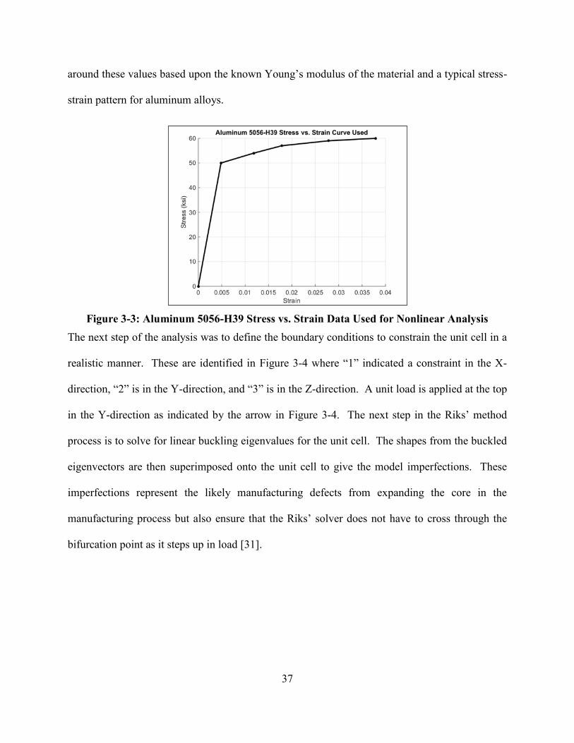
37

around these values based upon the known Young’s modulus of the material and a typical stress-

strain pattern for aluminum alloys.

Figure 3-3: Aluminum 5056-H39 Stress vs. Strain Data Used for Nonlinear Analysis

The next step of the analysis was to define the boundary conditions to constrain the unit cell in a

realistic manner. These are identified in Figure 3-4 where “1” indicated a constraint in the X-

direction, “2” is in the Y-direction, and “3” is in the Z-direction. A unit load is applied at the top

in the Y-direction as indicated by the arrow in Figure 3-4. The next step in the Riks’ method

process is to solve for linear buckling eigenvalues for the unit cell. The shapes from the buckled

eigenvectors are then superimposed onto the unit cell to give the model imperfections. These

imperfections represent the likely manufacturing defects from expanding the core in the

manufacturing process but also ensure that the Riks’ solver does not have to cross through the

bifurcation point as it steps up in load [31].

38

Figure 3-4: Unit Cell Model with Boundary Conditions and Load Applied (Boundary

Conditions Only Shown on Select Nodes along each edge for visual clarity)

After the imperfections have been smeared onto the model, modified Riks’ analysis is run in

Abaqus FEA and the deflected model contour plots are shown in Figure 3-5 and a stress-strain

curve derived from the model’s load versus displacement data is shown in Figure 3-6. This data

qualitatively agrees with Bianchi’s analysis on a different honeycomb core material type and

shows that Riks’ method is a good candidate for attempting to simulate the core failure of a more

complex joint coupon [27].

39

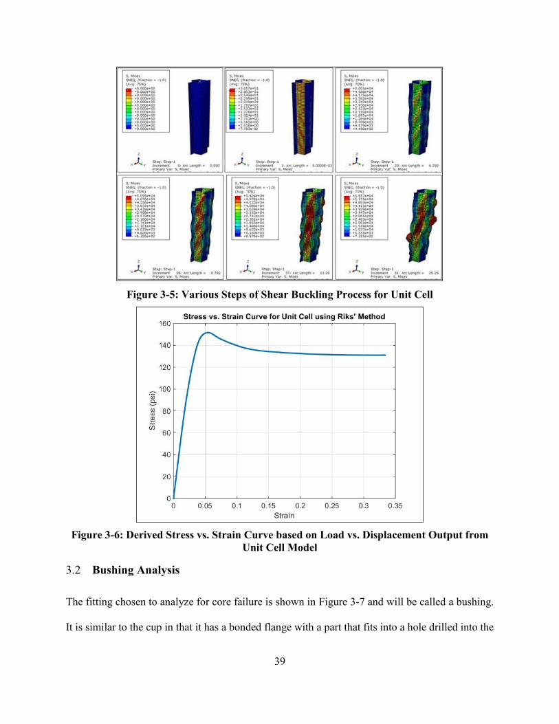
Figure 3-5: Various Steps of Shear Buckling Process for Unit Cell

Figure 3-6: Derived Stress vs. Strain Curve based on Load vs. Displacement Output from

Unit Cell Model

3.2 Bushing Analysis

The fitting chosen to analyze for core failure is shown in Figure 3-7 and will be called a bushing.

It is similar to the cup in that it has a bonded flange with a part that fits into a hole drilled into the

40

panel but differs in that it is not bonded to the inside of the opposite facesheet. It is instead held

by a separate flat fitting bonded to the other side of panel. The bushing coupon is also mounted

much closer to the edge of the panel than the cup coupon.

Figure 3-7: Images of Top and Bottom of Bushing Coupon

Six bushing coupons were tested with the load normal to the panel as shown in Figure 3-8. The

failure mode was core shear buckling as shown in the figure. Six coupons were tested until the

coupon lost load carrying capability as shown in Figure 3-9. Two of the coupons were tested

until complete failure where there was an adhesive disbond of the fitting but this happened at an

extremely high deflection that is not shown on the chart and is not relevant for this analysis.

41

Figure 3-8: Post-Test Image of Bushing Tested in Normal Direction

Figure 3-9: Load vs. Displacement Curves for Bushings Tested with Force Normal to Panel

The first step of the analysis process was to determine what a linear FEA model in NX Nastran

would predict for core failure. The cup model predicted the initiation of core failure accurately

in Chapter 2.3.2 but since it was a linear model it did not predict the change in slope caused by

this failure initiation. The linear model was created using the same modeling principles as used

in Section 2 and the model is shown in Figure 3-10. This model predicts a core shear initiation

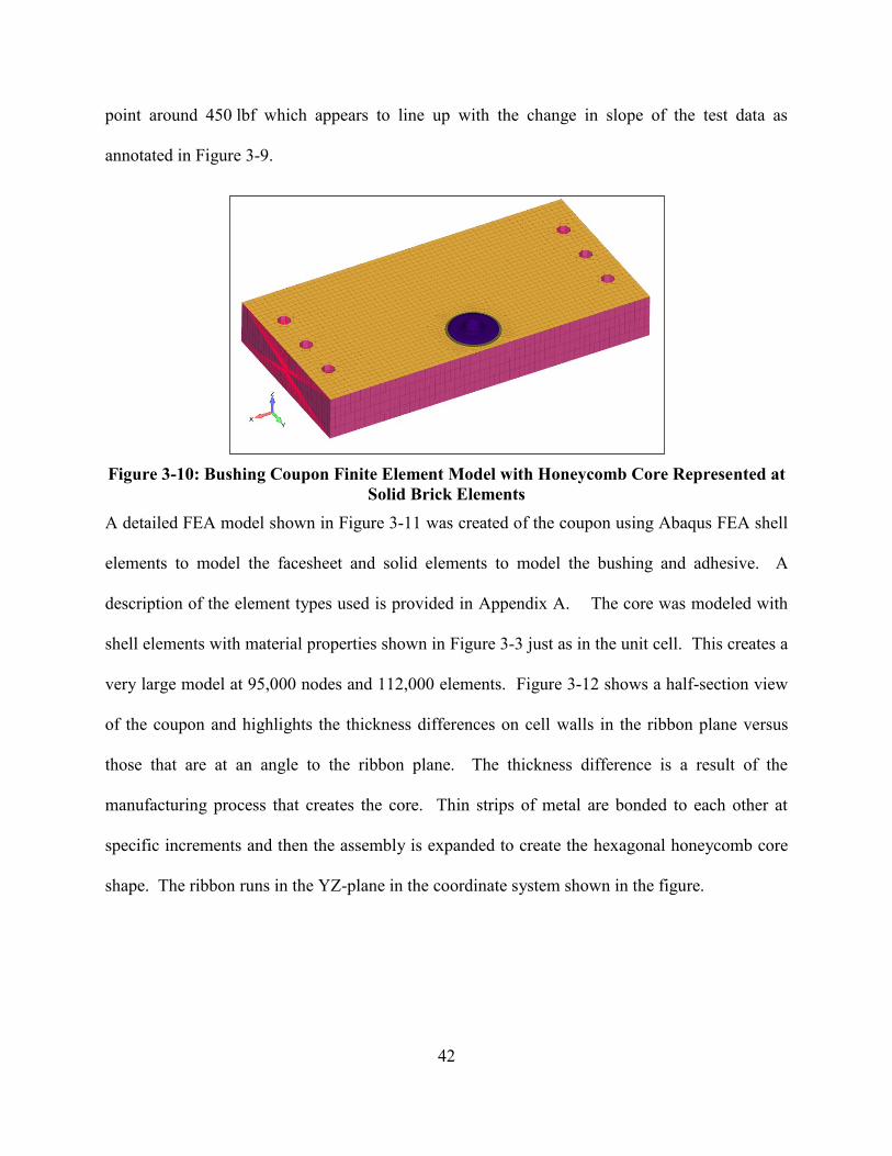
42

point around 450 lbf which appears to line up with the change in slope of the test data as

annotated in Figure 3-9.

Figure 3-10: Bushing Coupon Finite Element Model with Honeycomb Core Represented at

Solid Brick Elements

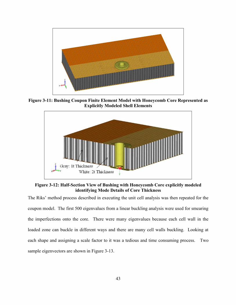
A detailed FEA model shown in Figure 3-11 was created of the coupon using Abaqus FEA shell

elements to model the facesheet and solid elements to model the bushing and adhesive. A

description of the element types used is provided in Appendix A. The core was modeled with

shell elements with material properties shown in Figure 3-3 just as in the unit cell. This creates a

very large model at 95,000 nodes and 112,000 elements. Figure 3-12 shows a half-section view

of the coupon and highlights the thickness differences on cell walls in the ribbon plane versus

those that are at an angle to the ribbon plane. The thickness difference is a result of the

manufacturing process that creates the core. Thin strips of metal are bonded to each other at

specific increments and then the assembly is expanded to create the hexagonal honeycomb core

shape. The ribbon runs in the YZ-plane in the coordinate system shown in the figure.

43

Figure 3-11: Bushing Coupon Finite Element Model with Honeycomb Core Represented as

Explicitly Modeled Shell Elements

Figure 3-12: Half-Section View of Bushing with Honeycomb Core explicitly modeled

identifying Mode Details of Core Thickness

The Riks’ method process described in executing the unit cell analysis was then repeated for the

coupon model. The first 500 eigenvalues from a linear buckling analysis were used for smearing

the imperfections onto the core. There were many eigenvalues because each cell wall in the

loaded zone can buckle in different ways and there are many cell walls buckling. Looking at

each shape and assigning a scale factor to it was a tedious and time consuming process. Two

sample eigenvectors are shown in Figure 3-13.

44

Figure 3-13: Images showing Sample Buckling Mode Shapes of the Coupon’s Honeycomb

Core

Riks’ method was then attempted but failed due to element aspect ratio errors as soon as the

model began to step into a nonlinear region. There were some relatively poorly formed elements

in the facesheet caused by having to mesh a circular bushing with a hexagonal honeycomb core

underneath it while trying to maintain even, square elements. After assessing at the geometry,

the fitting was remeshed but care was taken to make the model symmetric about the bushing and

also to locate the honeycomb core pattern in a location in the coupon Y-direction that was

conducive to achieving a workable mesh. The first mesh is shown in Figure 3-14 and the

updated, symmetric mesh is shown in Figure 3-15. The overall model remained about the same

size.

45

Figure 3-14: Original Mesh of Explicitly Modeled Honeycomb Core where Core was Not

Modeled Symmetric across the YZ-plane at the Center of the Bushing

Figure 3-15: Updated Mesh of Explicitly Modeled Honeycomb Core where Core was

Meshed Symmetric across the Bushing’s Center YZ-Plane

Riks’ method was then applied and the load versus displacement curve successfully simulated

the nonlinear region as shown in Figure 3-16. The core buckling was not triggered however and

instead the core simply yielded under the shear load as shown in Figure 3-17. The model was

also much stiffer than expected even in the linear region which can be seen by comparing the

slopes of the test data versus the predicted data. It should be noted that the displacement data in

the test was recorded by measuring the load head displacement on the test machine rather than by

using an extensometer. This means that the displacement in the model versus the test may be

46

different because the load head displacement will be increased albeit only slightly by the test

equipment in the load train rather than in just the coupon itself. An extensometer would have

mitigated this issue by isolating the coupon and is recommended for future coupon testing.

Figure 3-16: Bushing Coupon Test Data Compared against the Analytical Prediction from

the Coupon Model with Honeycomb Core Modeled Explicitly

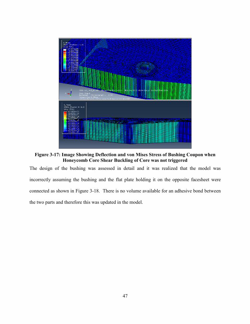
47

Figure 3-17: Image Showing Deflection and von Mises Stress of Bushing Coupon when

Honeycomb Core Shear Buckling of Core was not triggered

The design of the bushing was assessed in detail and it was realized that the model was

incorrectly assuming the bushing and the flat plate holding it on the opposite facesheet were

connected as shown in Figure 3-18. There is no volume available for an adhesive bond between

the two parts and therefore this was updated in the model.

48

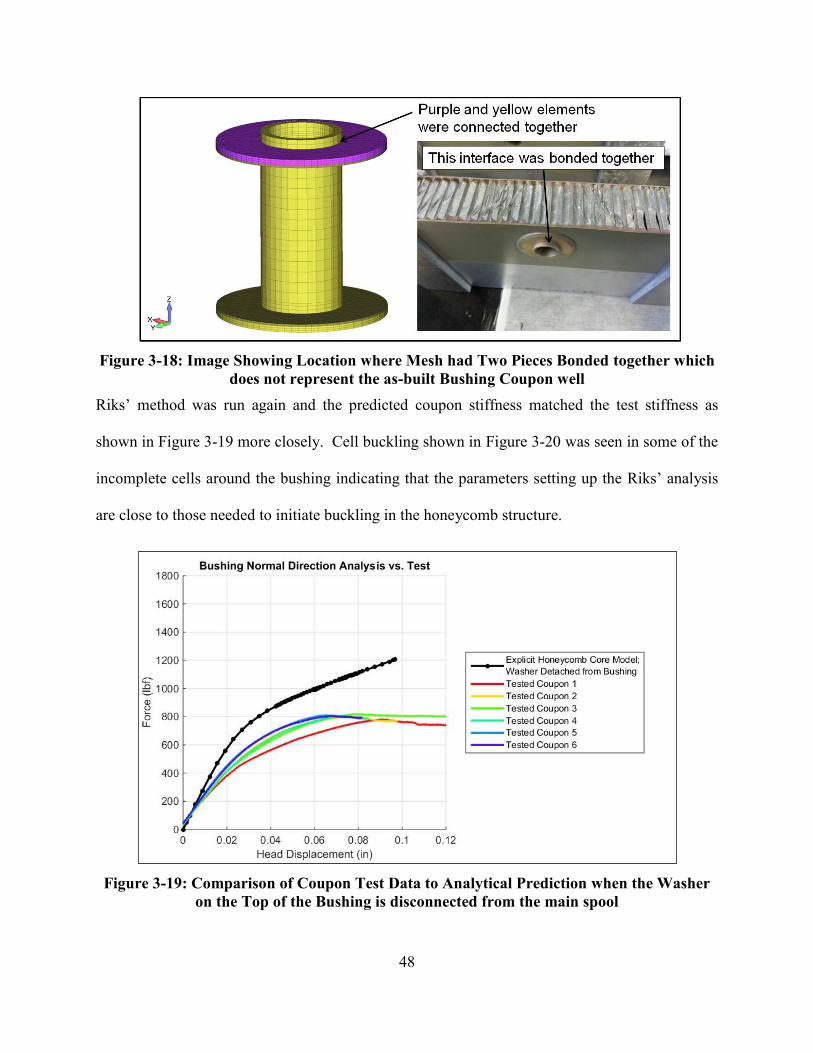
Figure 3-18: Image Showing Location where Mesh had Two Pieces Bonded together which

does not represent the as-built Bushing Coupon well

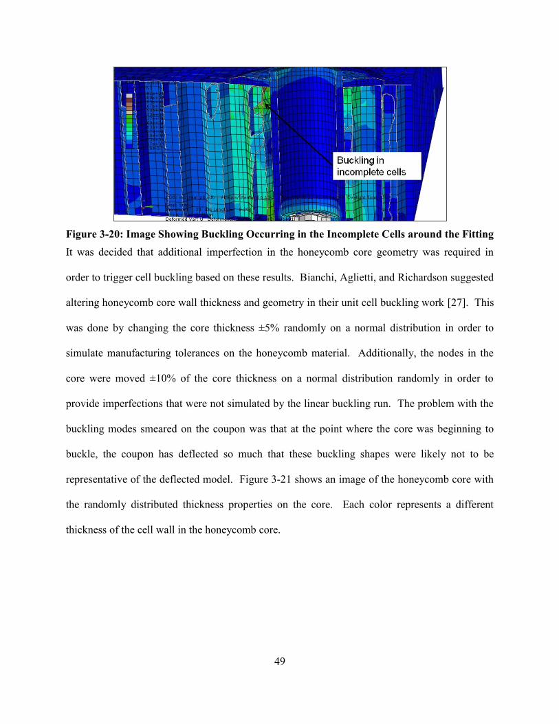
Riks’ method was run again and the predicted coupon stiffness matched the test stiffness as

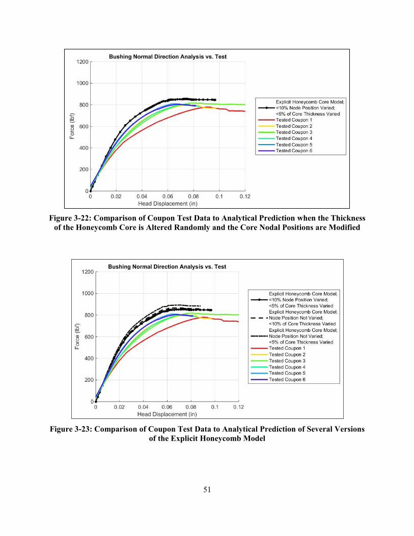
shown in Figure 3-19 more closely. Cell buckling shown in Figure 3-20 was seen in some of the

incomplete cells around the bushing indicating that the parameters setting up the Riks’ analysis

are close to those needed to initiate buckling in the honeycomb structure.

Figure 3-19: Comparison of Coupon Test Data to Analytical Prediction when the Washer

on the Top of the Bushing is disconnected from the main spool

49

Figure 3-20: Image Showing Buckling Occurring in the Incomplete Cells around the Fitting

It was decided that additional imperfection in the honeycomb core geometry was required in

order to trigger cell buckling based on these results. Bianchi, Aglietti, and Richardson suggested

altering honeycomb core wall thickness and geometry in their unit cell buckling work [27]. This

was done by changing the core thickness ±5% randomly on a normal distribution in order to

simulate manufacturing tolerances on the honeycomb material. Additionally, the nodes in the

core were moved ±10% of the core thickness on a normal distribution randomly in order to

provide imperfections that were not simulated by the linear buckling run. The problem with the

buckling modes smeared on the coupon was that at the point where the core was beginning to

buckle, the coupon has deflected so much that these buckling shapes were likely not to be

representative of the deflected model. Figure 3-21 shows an image of the honeycomb core with

the randomly distributed thickness properties on the core. Each color represents a different

thickness of the cell wall in the honeycomb core.

50

Figure 3-21: Image showing randomly Distributed Honeycomb Core Thickness Properties

across the coupon (Colors Represent Different Properties)

The updated model was successful in allowing the core to fail in shear buckling which caused a

load versus displacement curve that was very representative of the data from the coupon test as

seen in Figure 3-22. After the successful run, it was decided to check the sensitivity of the

results to the core thickness distribution and node locations. Figure 3-23 shows two additional

curves from Figure 3-22 with one having a ±10% core thickness distribution with no node

location altering and the other having a ±5% core thickness distribution with no node location

altering. Both of these models buckled and the results are very similar to the data obtained using

the core when the node locations were altered. Figure 3-24 shows an image of the coupon model

with the buckled honeycomb core in the Abaqus FEA viewer.

51

Figure 3-22: Comparison of Coupon Test Data to Analytical Prediction when the Thickness

of the Honeycomb Core is Altered Randomly and the Core Nodal Positions are Modified

Figure 3-23: Comparison of Coupon Test Data to Analytical Prediction of Several Versions

of the Explicit Honeycomb Model

52

Figure 3-24: Image Showing Buckled Honeycomb Core around Fitting

3.3 Discussion of Core Capability Analysis Results

The analysis using Riks’ method on the bushing coupon shows that it is possible to predict post-

buckling on a coupon with the core explicitly modeled. This analysis is much more complex and

the modeling is difficult due to the honeycomb core hexagonal shapes needing to be meshed in

conjunction with solid fittings which generally have square or circular shapes. The analysis also

requires a higher mesh quality than the linear FEA presented in Section 2 due to the nonlinear

effects but could be a useful tool an analyst believes that the core will be the ultimate driver of

joint capability rather than an adhesive bond.

A convergence study based on mesh size has not been performed for this analysis. The mesh

size used was based on giving as high quality of a mesh as possible in the facesheet. The

honeycomb mesh size was based on keeping shell elements as square as possible based on the

mesh size that had been used in the facesheet. The analysis was performed on a computer with a

3.5 GHz Xeon® processor with 32 GB of RAM. The linear buckling analysis on the 95,000

node and 112,000 element model took 30 minutes to solve and the post-buckling run took 10

hours to solve.

53

4 Conclusions

This thesis showed that predicting joint capability using FEA is possible for a honeycomb panel

and coupon testing early in a program to determine joint capability can be avoided. This chapter

will provide a succinct overview of the methodology used and the analytical results. The chapter

will then provide conclusions about the results and discuss future opportunities for improvement

and expansion of the analysis.

4.1 Overview and Conclusions

This thesis’ primary purpose was to show that finite element analysis can be used to predict

honeycomb joint capability with reasonable accuracy. The thesis started by using linear FEA in

NX Nastran to show that an adhesive bondline’s capability can be predicted accurately if the

model is setup properly and the results are interpreted carefully. The finite element model must

be setup by creating as regular a mesh as possible and by using at least three solid elements

through the thickness of the adhesive in order for the model to predict local stress gradients.

Additionally, in order to mitigate the effect of the singularity created by the large stiffness

difference between the soft adhesive and the stiff adherents, an additional row of elements must

be modeled beyond the free edge of the bond.

The finite element model is then submitted to NX Nastran to run using a linear static solution

which allows for low run times. The results from the run must then be interpreted by the analyst

carefully. First, all relevant failure modes should be identified and each mode’s allowable

compared to the failure loads predicted by the model. The analyst must then step through each

failure mode and determine if the failure will cause a catastrophic failure in the joint or if the

joint will continue to carry load. The thesis used this method on a cup joint and an H-Clip joint

54

and showed that the joint capability predictions determined using this method compare very well

to coupon test data of the joint.

The second portion of the thesis was also dedicated to determining joint capability but the focus

shifted from determining the adhesive bondline capability to predicting core failure using

nonlinear analysis in Abaqus FEA. This was done because while it was shown that the linear

models with the core modeled using homogenous brick elements could predict when the core

would begin to fail, the joint was able to continue to carry significant load as the core buckled

and the load versus displacement curve became nonlinear.

The finite element model for performing the nonlinear analysis is very demanding, and creating

and maintaining a good mesh quality is very important so that Abaqus can step through the

nonlinear post-buckling solution using the modified Riks’ method. The honeycomb cells were

modeled explicitly using S4 shell elements. The Riks’ method requires that imperfections be

included in the post-buckling run. These were included by smearing buckled shape eigenvectors

onto the mesh as well as including a randomly distributed thickness variation in the core. The

use of modified Riks’ analysis as implemented in Abaqus was instrumental in successfully

performing the nonlinear post-buckling analysis of a honeycomb coupon to predict the ultimate

core failure with good accuracy.

4.2 Future Work

The linear FEA was able to predict the joint capability accurately but required careful

interpretations of the results to do so. For both the cup and H-Clip model, one of the bondlines

was predicted to fail below the actual joint capability but it was clear from the geometry that the

bondline on the other facesheet could continue to carry the load. There are likely examples of

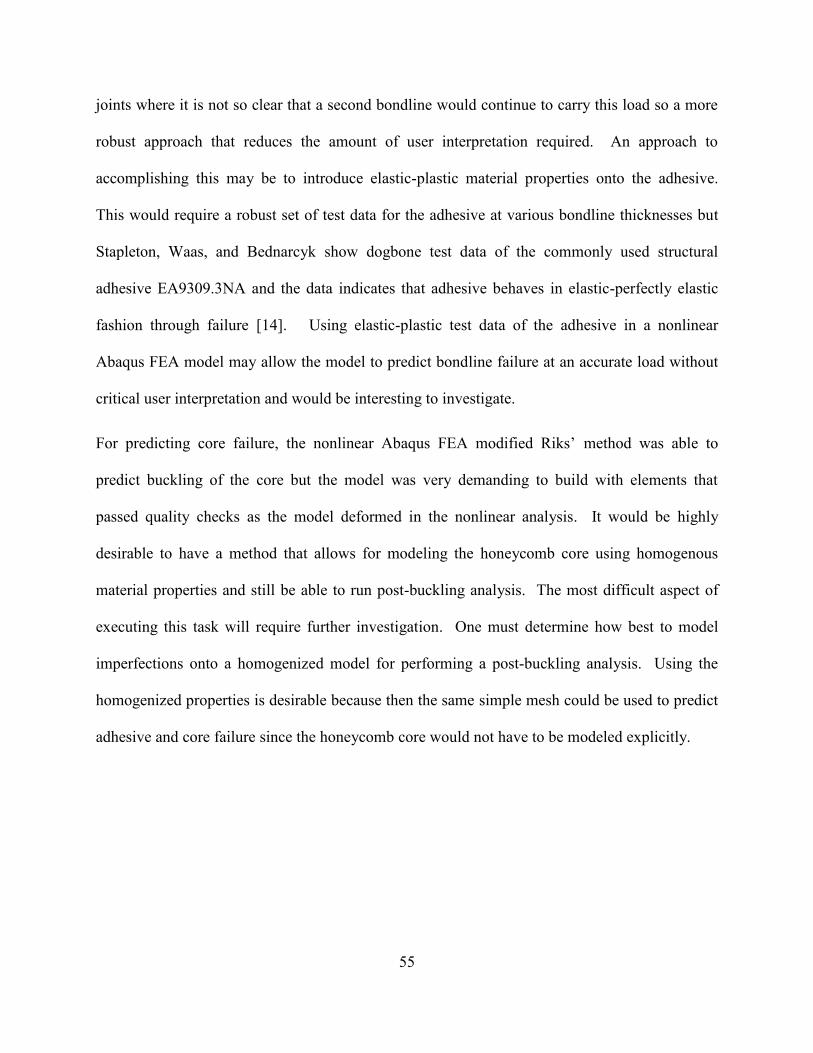
55

joints where it is not so clear that a second bondline would continue to carry this load so a more

robust approach that reduces the amount of user interpretation required. An approach to

accomplishing this may be to introduce elastic-plastic material properties onto the adhesive.

This would require a robust set of test data for the adhesive at various bondline thicknesses but

Stapleton, Waas, and Bednarcyk show dogbone test data of the commonly used structural

adhesive EA9309.3NA and the data indicates that adhesive behaves in elastic-perfectly elastic

fashion through failure [14]. Using elastic-plastic test data of the adhesive in a nonlinear

Abaqus FEA model may allow the model to predict bondline failure at an accurate load without

critical user interpretation and would be interesting to investigate.

For predicting core failure, the nonlinear Abaqus FEA modified Riks’ method was able to

predict buckling of the core but the model was very demanding to build with elements that

passed quality checks as the model deformed in the nonlinear analysis. It would be highly

desirable to have a method that allows for modeling the honeycomb core using homogenous

material properties and still be able to run post-buckling analysis. The most difficult aspect of

executing this task will require further investigation. One must determine how best to model

imperfections onto a homogenized model for performing a post-buckling analysis. Using the

homogenized properties is desirable because then the same simple mesh could be used to predict

adhesive and core failure since the honeycomb core would not have to be modeled explicitly.

56

Bibliography

[1] Dattaguru, B., Everett, R.A., Whitcomb, J.D., Johnson, W.S., "Geometrically Nonlinear

Analysis of Adhesively Bonded Joints," Journal of Engineering Materials and

Technology, Vol 106, No. 59, pp. 59-65, 1984.

[2] Volkersen, O., Die Niektraftverteilung in Zugbeanspruchten mit Konstanten

Laschenquerschritten, Luftfahrtforschung 15, 1938, pp. 41-47.

[3] M. Goland and E. Reissner, “The Stresses in Cemented Joints,” Journal of Applied

Mechanics 11, 1944, pp. A17-A27.

[4] Hart-Smith, L.J., "Designing to Minimize Peel Stresses in Adhesive-Bonded Joints,"

ASTM Symposium on Delamination and Debonding of Materials, November 8-10,

1983, Pittsburgh, Pennsylvania, Douglas Paper 7389.

[5] Adams, R.D., Peppiatt, N.A., "Stress Analysis of Adhesive-Bonded Lap Joints," Journal

of Strain Analysis, Vol. 9, No. 3, pp. 185-196, 1974.

[6] Oplinger, D.W., "Effects of Adhered Deflections in Single Lap Joints," International

Journal of Solids and Structures, Vol. 31, No. 18, pp. 2565-2587, 1994.

[7] Derewońko, A., "Prediction of the Failure Metal/Composite Bonded Joints," Composite

Materials Science, Vol. 45, No. 3, May 2009, pp. 735-738, 2009.

[8] Zhu, Y., Kedward, K., "Methods of Analysis and Failure Predictions for Adhesively

Bonded Joints of Uniform and Variable Bondline Thickness," National Technical

57

Information Service, May 2005, Springfield, Virginia, DOT/FAA/AR-05/12.

[9] Barroso, A., París, F., Mantiĉ, V., "Representativity of the Singular Stress State in the

Failure of Adhesively Bonded Joints between Metals and Composites," Composites

Science and Technology, Vol. 69, No. 11-12, pp. 1746-1755, 2009.

[10] Gonçalves, J.P.M., de Moura, M.F.S.F., de Castro, P.M.S.T., "A Three-Dimensional

Finite Element Model for Stress Analysis of Adhesive Joints," International Journal of

Adhesion & Adhesives, Vol. 22, No. 5, pp. 357-365, 2002.

[11] Reddy, J.N., "An Introduction to the Finite Element Method, Third Edition," McGraw

Hill, Boston, Massachusetts, 2005.

[12] Lundgren, E.C., Smeltzer III, S.S., Kapania, R.K., "Durable Joining Technology for

Uniformly-Curved Composite Sandwich Structures," 51st AIAA/ASCE/AHS/ASC

Structures, Structural Dynamics, and Materials Conference, AIAA 2010-2779.

[13] Osnes, H., Anderson, A., "Computational Analysis of Geometric Nonlinear Effects in

Adhesively Bonded Single Lap Composite Joints," Composites Part B: Engineering,

Vol. 34, No. 5, pp. 417-427, 2003.

[14] Stapleton, S.E., Waas, A.M., "Modeling Progressive Failure of Bonded Joints Using a

Single Joint Finite Element," 51st AIAA/ASME/ASCE/AHS/ASC Structures,

Structural Dynamics, and Materials Conference, April 2010, AIAA 2010-3100.

[15] Ficarra, C.H., "Analysis of Adhesive Bonded Fiber-Reinforced Composite Joints," North

58

Carolina State University, Raleigh, North Carolina, 2001.

[16] da Silva, L.F.M., Campilho, R.D.S.G., "Advances in Numerical Modeling of Adhesive

Joints," Springer Briefs in Computational Mechanics, 2012, 10.1007/978.

[17] Hinopoulos, G., Broughton, W.R., "Evaluation of the T-peel Joint Using the Finite

Element Method," National Physical Laboratory, Teddington, Middlesex, UK, 1999,

ISSN 1361-4061.

[18] He, X., "Influence of Boundary Conditions on Stress Distributions in a Single-Lap

Adhesively Bonded Joint," International Journal of Adhesion and Adhesives, Vol. 53,

pp. 34-43, 2014.

[19] Devadas, N.P., Sunikumar, G., Sajeeb, R., "Finite Element Analysis of Flat Joints in

Honeycomb Sandwich Beams," Journal of Mechanical and Civil Engineering, Vol. 3,

No. 2, pp. 06-12, 2012.

[20] Callister, W.D., Rethwisch, D.G., "Fundamentals of Materials Science and Engineering,

Third Edition," John Wiley & Sons, Inc. Hoboken, New Jersey, 2008.

[21] Groover, M.P., "Fundamentals of Modern Manufacturing: Materials, Processes, and

Systems, 4th Edition," John Wiley & Sons, Hoboken, New Jersey, 2010.

[22] Petras, A., Sutcliffe, M.P.F., "Failure Mode Maps for Honeycomb Sandwich Panels,"

Composite Structures, Vol. 44, No. 4, pp. 237-252, 1999.

[23] Young, W.C., Budynas, R.G., Sadegh, A.M., "Roark's Formulas for Stress and Strain,

59

8th Edition," McGraw Hill, New York, 2012.

[24] Heimbs, S., Pein, M., "Failure of Honeycomb Sandwich Corner Joints and Inserts,"

Composite Structures, Vol. 89, No. 4, August 2009, pp. 575-588, 2009.

[25] Ferrari, M., "Structurally Optimized and Additively Manufactured Inserts for Sandwich

Panels of Spacecraft Structures," Swiss Federal Institute of Technology Zurich,

Master's thesis no. 15-039, 2015.

[26] Bianchi, G., Aglietti, G.S., Richardson, G., "Experimental Investigation of Static and

Fatigue Behaviour of Honeycomb Panels under In-Plane Shear Loads," 50th

AIAA/ASME/ASCE/AHS/ASC Structures, Structural Dynamics, and Materials

Conference, May 2009, AIAA 2009-2674.

[27] Bianchi, G., Aglietti, G.S., Richardson, G., "Static and Fatigue Behaviour of Hexagonal

Honeycomb Cores under In-Plane Shear Loads," Applied Composite Materials, Vol.

19, No. 2, pp. 97-115, 2012.

[28] Stoumbos, T., Lyford, A., Setoodeh, S., Curtis, D., Adhesively Bonded Joint Modeling

using Finite Element Method for Failure Mode Prediction," 55th

AIAA/ASME/ASCE/AHS/ASC Structures, Structural Dynamics, and Materials

Conference, AIAA SciTech Forum, AIAA 2014-1531

[29] Lyford, A., Stoumbos, T., Kapania, R.K., "Adhesively Bonded Joint Modeling

Approaches using Linear Finite Element Analysis", 56th AIAA/ASCE/AHS/ASC

Structures, Structural Dynamics, and Materials Conference, AIAA SciTech Forum,

60

AIAA 2015-1883.

[30] Loss, K.R., Kedward, K.T., "Modeling and analysis of peel and shear stresses in

adhesively bonded joints", 25th Structures, Structural Dynamics and Materials

Conference, Structures, Structural Dynamics, and Materials. AIAA 1984-913.

[31] Zhao, M., "On Nonlinear Buckling and Collapse Analysis using Riks Method," Abaqus

User's Conference, 2008.

[32] Siemens Product Lifecycle Management Software, "NX Nastran 8 Element Library

Reference," 2011.

[33] Dassault Systemes, "Abaqus 6.13, Analysis User's Guide, Volume IV: Elements,"

Providence, Rhode Island, 2013.

61

Appendix A: Element Usage Details

A.1 NX Nastran Model Elements

The cup and H-Clip models discussed in Section 2 of this report used NX Nastran 8.5 to run the

analysis and used the same element types to model features. This section will discuss which

element types were used specifically in the models. Figure A-1 shows the H-Clip model from

Section 2 with the element types identified. The main components in the model are the fitting,

honeycomb core, adhesive and the panel facesheet.

Figure A-1: H-Clip Fitting Model with NX Nastran Element Types Identified

The panel facesheet was modeled using CQUAD4 shell elements. These elements have 4 nodes

on the corners. Due to meshing limitations, some CTRIA3 shell elements were used but these

are all in the far-field from the fitting in the mesh transition region going to the edge boundary

conditions and so they are not focused on here. There are 14 CTRIA3 elements versus over 6000

CQUAD4 elements in this model for comparison. The NX Nastran CQUAD4 and CTRIA3

62

elements are based on Mindlin-Reissner shell theory and are recommended for modeling flat

geometry such as the panel’s facesheets [32]. Additionally, the 4-node CQUAD4 element is

recommended over the 8-node higher-order CQUAD8 element for flat plates. The CQUAD8

element is acknowledged to be more accurate but this effect is negligible on flat geometry and

the CQUAD8 element increases the computational task for NX Nastran [32]. The stress

calculations for these elements were not critical for these problems as the failures are driven by

the adhesives and the core.

The honeycomb core, adhesive and the fitting are each modeled using solid six-sided CHEXA

elements with a few wedge-shaped CPENTA elements in the honeycomb core in the far-field

from the adhesive. The CPENTA elements are at the same locations in the X-Y plane as the

CTRIA3 elements in the facesheet. The solid element types were used for the fittings because of

their complex geometry that were not conducive to shell element model and for the core and

adhesive so stress variation could be captured through the thickness of the adhesive. The 8-node

CHEXA and 6-node CPENTA element type were used with their default integration point

scheme which uses reduced integration. This formulation minimizes shear-locking in the

element and eliminates the mesh instability that can arise in some element formulations known

as hourglassing where element strain erroneously decouples itself from element deformation

[32]. The stress used for failure margin calculations is output at the center of the element.

The final element type used is an RBE2 rigid element that is used to represent the rigid bolted

connection where the load is applied to the coupon. This is not actually an element but an

automated multi-point constraint (MPC) capability that is provided by NX Nastran [32]. The

MPC equations eliminate the degrees of freedom of all nodes on the dependent side of the

63

element and wrap them up into the node on the independent side of the element hence why the

element is referred to as a rigid element.

A.2 Abaqus FEA Model Elements

The bushing model discussed in Section 3 of this report used Abaqus FEA 6.13 to run the

analysis. This section will discuss which element types were used in the model and provide

rationale as to why they are acceptable. Abaqus FEA provides significantly more element

choices and formulations than NX Nastran and therefore careful consideration must be given to

each element type. Figure A-2 shows a half-section view of the bushing model with element

types identified for each component.

Figure A-2: Bushing Model with Abaqus FEA Element Types Identified

The bushing and adhesive models are only needed to transmit the load to the coupon accurately

in this model as adhesive is not a potential failure mode. Because of this and to reduce the

complexity of the model, C3D6R and C3D8R reduced integration solid elements were used to

model these components. The reduced integration element minimizes the number of integration

64

points which can lead to hourglassing if not used properly. Abaqus FEA recommends using a

fine mesh in addition to its default hourglass control settings to prevent this hourglassing which

was done in the model with at least 3 elements through the thickness of each component [33].

Additionally, in order to prevent hourglassing from occurring at the load application point in the

middle of the bushing, kinematic coupling was used to spread the load out in a similar manner to

the RBE2 element in Section A.1. No hourglassing was observed in any elements in the model

and therefore this element type was sufficient.

The panel facesheets were modeled using S3R and S4R reduced-integration shell elements. The

facesheet like the adhesive and fitting was not expected to contribute to the failure of the fitting

and therefore the less-expensive reduced integration elements were used. S4R elements were

used when the mesh allowed but the 3-node triangular S3R elements were required in areas

where it was only possible to put a highly distorted S4R element. These elements have one

integration point at the center and no hourglassing was observed due to the fine mesh and using

Abaqus FEA’s default hourglass control settings [33].

The honeycomb core which was modeled explicitly is where failure was expected to and did

occur in the Riks’ method analysis. Because of this expectation, S4 shell elements were used for

modeling. While these 4 integration point elements are more computationally expensive than

1 integration point S4R elements, they are superior to them in that they cannot hourglass and are

recommended for areas where significant bending is expected such as in the core as it buckles

[33]. No triangular S3 elements were required in the core because the elements were extruded

down from the facesheet mesh and all elements were given dimensions as close to square as

possible to aid in the solution accuracy. Based on the results, the S4 elements contributed as

expected to the model.