Fading Channels: Capacity, BER and Diversity - … · I Fading channels: The instantaneous ... 1.Shannon’s coding theorem proves that a code exists that ... Fading Channels: Capacity,

Fading Channels: Capacity, BER and Diversity

Master Universitario en Ingenierıa de Telecomunicacion

I. Santamarıa

Universidad de Cantabria

Introduction Capacity BER Diversity Conclusions

Contents

Introduction

Capacity

BER

Diversity

Conclusions

Fading Channels: Capacity, BER and Diversity 0/48


Introduction

I We have seen that the randomness of signal attenuation(fading) is the main challenge of wireless communicationsystems

I In this lecture, we will discuss how fading affects

1. The capacity of the channel2. The Bit Error Rate (BER)

I We will also study how this channel randomness can be usedor exploited to improve performance → diversity



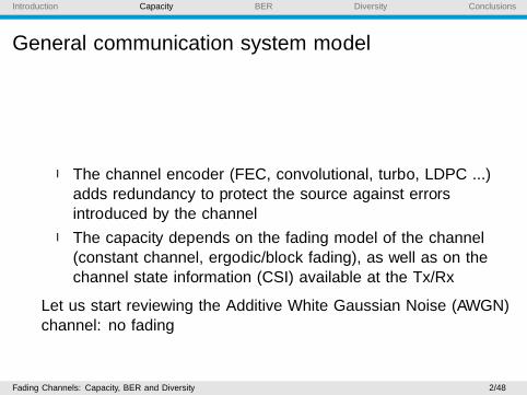
General communication system model

Source ChannelModulator ⊕

Noise

Demod.

][ns][ns][nb ][nbChannelDecoder

ChannelEncoder

I The channel encoder (FEC, convolutional, turbo, LDPC ...)adds redundancy to protect the source against errorsintroduced by the channel

I The capacity depends on the fading model of the channel(constant channel, ergodic/block fading), as well as on thechannel state information (CSI) available at the Tx/Rx

Let us start reviewing the Additive White Gaussian Noise (AWGN)channel: no fading



AWGN Channel

I Let us consider a discrete-time AWGN channel

y [n] = hs[n] + r [n]

where r [n] is the additive white Gaussian noise, s[n] is thetransmitted signal and h = |h|e jθ is the complex channel

I The channel is assumed constant during the reception of thewhole transmitted sequence

I The channel is known to the Rx (coherent detector)

I The noise is white and Gaussian with power spectral densityN0/2 (with units W/Hz or dBm/Hz, for instance)

I We will mainly consider passband modulations (BPSK, QPSK,M-PSK, M-QAM), for which if the bandwith of the lowpasssignal is W the bandwidth of the passband signal is 2W



Signal-to-Noise-Ratio

I Transmitted signal power: P

I Received signal power: P|h|2I Total noise power: N = 2WN0/2 = WN0

I The received SNR is

SNR = γ =P|h|2WN0

I In terms of the energy per symbol P = Es/Ts

I We assume Nyquist pulses with β = 1 (roll-off factor) soW = 1/Ts

I Under these conditions

SNR =EsTs |h|2TsN0

=Es |h|2N0



I For M-ary modulations, the energy per bit is

Eb =Es

log(M)⇒ SNR =

Eb|h|2N0 log(M)

I To model the noise we generate zero-mean circular complexGaussian random variables with σ2 = N0

r [n] ∼ CN(0, σ2) or r [n] ∼ CN(0,N0)

I The real and imaginary parts have variance

σ2I = σ2

Q =σ2

2=

N0

2



Average SNR and Instantaneous SNR

Sometimes, we will find useful to distinguish between the averageand the instantaneous signal-to-noise ratio

Average⇒ SNR = γ =P

WN0

Instantaneous⇒ SNR = γ|h|2 =P

WN0|h|2

I AWGN channel: N0 and h are assumed to be known(coherent detection), therefore we typically take (w.l.o.g)h = 1 ⇒ SNR = γ = P

WN0, and the SNR at the receiver is

constant

I Fading channels: The instantaneous signal-to-noise-ratioSNR = γ = γ|h|2 is a random variable



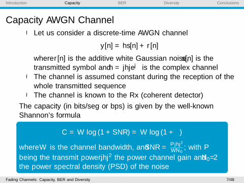
Capacity AWGN ChannelI Let us consider a discrete-time AWGN channel

y [n] = hs[n] + r [n]

where r [n] is the additive white Gaussian noise, s[n] is thetransmitted symbol and h = |h|e jθ is the complex channel

I The channel is assumed constant during the reception of thewhole transmitted sequence

I The channel is known to the Rx (coherent detector)

The capacity (in bits/seg or bps) is given by the well-knownShannon’s formula

C = W log (1 + SNR) = W log (1 + γ)

where W is the channel bandwidth, and SNR = P|h|2WN0

; with P

being the transmit power, |h|2 the power channel gain and N0/2the power spectral density (PSD) of the noise



I Sometimes, we will find useful to express C in bps/Hz (orbits/channel use)

C = log (1 + SNR)

A few things to recall

1. Shannon’s coding theorem proves that a code exists thatachieves data rates arbitrarily close to capacity withvanishingly small probability of bit error

I The codewords might be very long (delay)I Practical (delay-constrained) codes only approach capacity

2. Shannon’s coding theorem assumes Gaussian codewords, butdigital communication systems use discrete modulations(PSK,16-QAM)



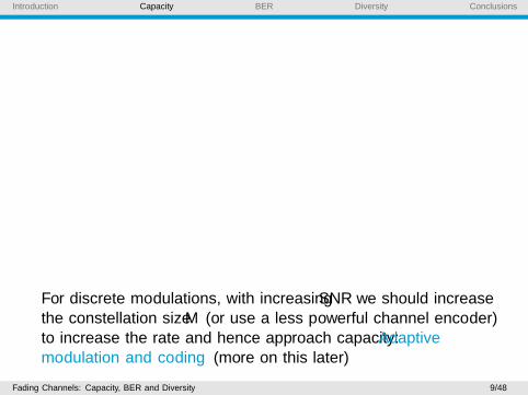
5 10 15 20 25 30SNR dB

0

2

4

6

8

10

Cap

acity

(bp

s/H

z)64-QAM

16-QAM

4-QAM (QPSK)

Gaussian inputs log(1+SNR)

Shaping gain (1.53 dB)

Pe (symbol) = 10-6 (uncoded)

For discrete modulations, with increasing SNR we should increasethe constellation size M (or use a less powerful channel encoder)to increase the rate and hence approach capacity: Adaptivemodulation and coding (more on this later)



Capacity fading channelsI Let us consider the following example1

AWGNC = 2 bps/Hz

AWGNC = 1 bps/Hz

ChannelEncoder

RandomSwitch

Fading channel

I The channel encoder is fixedI The switch takes both positions with equal probabilityI We wish to transmit a codeword formed by a long sequence of

coded bits, which are then mapped to symbolsI What is the capacity for this channel?1Taken from E. Biglieri, Coding for Wireless Communications, Springer,

2005Fading Channels: Capacity, BER and Diversity 10/48


The answer depends on the rate of change of the fading

1. If the switch changes position every symbol period, thecodeword experiences both channels with equal probabilitiesso we could use a fixed channel encoder, and transmit at amaximum rate

C =1

2C1 +

1

2C2 = 1.5 bps/Hz

2. If the switch remains fixed at the same (unknown) positionduring the transmission of the whole codeword, then we shoulduse a fixed channel encoder, and transmit at a maximum rate

C = C1 = 1 bps/Hz

or otherwise half of the codewords would be lost



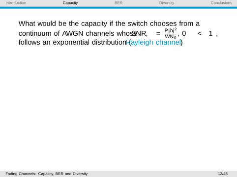
What would be the capacity if the switch chooses from a

continuum of AWGN channels whose SNR, γ = P|h|2WN0

, 0 ≤ γ <∞,follows an exponential distribution (Rayleigh channel)

ChannelEncoder

RandomSwitch

)1log( 11 γ+=C

)1log( 22 γ+=C

)1log( 33 γ+=C



Fast fading (ergodic) channel

I If the switch changes position every symbol period, and thecodeword is long enough so that the transmitted symbolsexperience all states of the channel (fast fading or ergodicchannel)

C = E [log(1 + γ)] =

∫ ∞0

log(1 + γ)f (γ)dγ (1)

where f (γ) = 1γ e−γ/γ , with γ being the average SNR

I Eq. (1) is the ergodic capacity of the fading channel

I For Rayleigh channels the integral in (1) is given by

C =1

2 ln(2)exp

(1

γ

)E1

(1

γ

)where E1(x) =

∫∞x

e−tt dt is the Exponential integral function2

2y=expint(x) in MatlabFading Channels: Capacity, BER and Diversity 13/48


I The ergodic capacity is in general hard to compute in closedform (we can always resort to numerical integration)

I We can apply Jensen’s inequality to gain some qualitativeinsight into the effect of fast fading on capacity

Jensen’s inequality

If f (x) is a convex function and X is a random variable

E [f (X )] ≥ f (E [X ])

If f (x) is a concave function and X is a random variable

E [f (X )] ≤ f (E [X ])

I log(·) is a concave function, therefore

C = E [log(1 + γ)] ≤ log (1 + E [γ]) = log (1 + γ)



The capacity of a fading channel with receiver CSI is less than thecapacity of an AWGN channel with the same average SNR

'

&

$

%

SISO Fading Channel: Ergodic Capacity

Assume iid Rayleigh fading with σ2h = E[|h|2] = 1, and σ2

z = 1.

−10 −5 0 5 10 15 200

1

2

3

4

5

6

7

SNR (dB)

Cap

acity

(bp

s/H

z)

AWGN Channel CapacityFading Channel Ergodic Capacity

17Fading Channels: Capacity, BER and Diversity 15/48


Block fading channel

I If the switch remains fixed at the same (unknown) positionduring the transmission of the whole codeword, there is nononzero rate at which long codewords can be transmitted withvanishingly small probability or error

I Strictly, the capacity for this channel model would be zero

I In this situation, it is more useful to define the outagecapacity

Cout = r ⇒ Pr(log(1 + γ) < r) = Pr(C (h) < r) = Pout

Suppose we transmit at a rate Cout with probability of outagePout = 0.01 this means that with probability 0.99 theinstantaneous capacity of the channel (a realization of a r.v.) willbe larger than rate and the transmission will be successful; whereaswith probability 0.01 the instantaneous capacity will be lower thanthe rate and the all bits in the codeword will be decoded incorrectly



I Pout is the error probability since data is only correctlyreceived on 1− Pout transmissions

I What is the outage probability of a block fading Rayleighchannel with average SNR = γ for a transmission rate r?

Pout = Pr(log(1 + γ) < r)

I The rate is a monotonic increasing function with theSNR = γ; therefore, there is a γmin needed to achieve the rate

log(1 + γmin) = r ⇒ γmin = 2r − 1

and Pout can be obtained as

Pout =Pr(γ < γmin) =

∫ γmin

0f (γ)dγ =

∫ γmin

0

1

γe−γ/γdγ =

=1− e−γminγ = 1− e−

2r−1γ



Pout vs Cout (rate) for γ = 100 (10 dB)

Pout

10-4 10-3 10-2

Rat

e (b

ps/H

z)

0

0.2

0.4

0.6

0.8

1



Summary

L

1h

L

L

1h 1h

L

1h

L

L

2h nh

1h

L

1h L

2h Lh2h Lh

AWGN

Ergodic (fast fading)

Block fading

)]1[log( γ+= EC

)1log( γ+=C

outageC



Final note

I All capacity results seen so far correspond to the case ofperfect CSI at the receiver side (CSIR)

I If the transmitter also knows the channel, we can performpower adaptation and the results are different

I We’ll see more on this later

Now, let’s move to analyze the impact of fading on the Bit ErrorRate (BER)



BER analysis for the AWGN channel (a brief reminder)

I BPSK s[n] ∈ {−1,+1}

Ps = Pb = Q

(√2Es

N0

)= Q

(√2SNR

)where Q(x) =

∫∞x

1√2π

exp−(x2/2) ≤ 12 exp−(x2/2)

I QPSK s[n] ∈ {−1−j√2, −1+j√

2, 1−j√

2, 1+j√

2}

Ps = 1−(

1− Q(√

SNR))2

I Nearest neighbor approximation Ps ≈ 2Q(√

SNR)

I With Gray encoding Pe = Ps/2



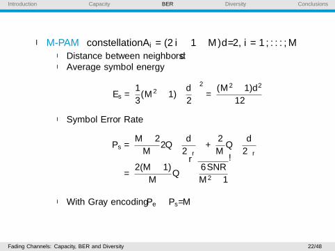
I M-PAM constellation Ai = (2i − 1−M)d/2, i = 1, . . . ,MI Distance between neighbors: dI Average symbol energy

Es =1

3(M2 − 1)

(d

2

)2

=(M2 − 1)d2

12

I Symbol Error Rate

Ps =M − 2

M2Q

(d

2σr

)+

2

MQ

(d

2σr

)=

2(M − 1)

MQ

(√6SNR

M2 − 1

)I With Gray encoding Pe ≈ Ps/M



I M-QAM: the constellations for the I and Q branches areAi = (2i − 1−M)d/2, i = 1, . . . ,M

I At the I and Q branches we have orthogonal√M − PAM

signals, each with half the SNR

I Symbol Error Rate

Ps = 1−(

1− 2(√M − 1)√M

Q

(√3SNR

M − 1

))2

I Nearest neighbor approximation (4 nearest neighbors)

Ps ≈ 4Q

(√3 SNR

M − 1

)



The impact of fading on the BER

I Let us consider for simplicity a SISO channel with a BPSKsource signal

x [n] = hs[n] + r [n]

s[n] ∈ {+1,−1}, r [n] ∼ CN(0, σ2) is the noise (additive,white and Gaussian)

I An AWGN channel or a fading channel behave also differentlyin terms of BER

AWGN channel: h is constant

h

Rayleigh fading channel: h ~ CN(0,1)

h



I The receiver knows perfectly the channel → coherent det.I Since we are sending a BPSK signal over a complex channel

the optimal coherent detector is

Re

(h∗x [n]

|h|

)+1≷−1

0 (2)

I Assuming that the transmitted power is normalized to unityE [|s[n]|2] = 1, the average SNR is

SNR =1

σ2

and the instantaneous Signal-to-Noise-Ratio is SNR|h|2I For an AWGN channel, SNR|h|2 is a constant value and the

BER is

Pe = Q

(√2|h|σ

)= Q

(√2|h|2SNR

)where Q(x) =

∫∞x

1√2π

exp−(x2/2) ≤ 12 exp−(x2/2)



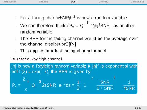
I For a fading channel SNR|h|2 is now a random variable

I We can therefore think of Pe = Q(√

2|h|2SNR)

as another

random variable

I The BER for the fading channel would be the average overthe channel distribution E [Pe ]

I This applies to a fast fading channel model

BER for a Rayleigh channel

|h| is now a Rayleigh random variable (z = |h|2 is exponential withpdf f (z) = exp(−z), the BER is given by

Pe =

∫ ∞0

Q(√

2zSNR)e−zdz =

1

2

(1−

√SNR

1 + SNR

)≈ 1

4SNR



0 2 4 6 8 10 12 14 16

10−10

10−8

10−6

10−4

10−2

100

SNR (dB)

BER

AWGNRayleigh

At an error probability of Pe = 10−3, a Rayleigh fading channelneeds 17 dB more than an AWGN (constant) channel, even thoughwe have perfect channel knowledge in both cases !!



I The main reason of the poor performance is that there is asignificant probability that the channel is in a deep fade, andnot because of noise

I The instantaneous signal-to-noise-ratio is |h|2SNR, and wemay consider that the channel is in a deep fade when|h|2SNR < 1

I In this event, the separation between constellation points willbe of the order of magnitude of σ (noise standard deviation)and the probability of error will be high

I For a Rayleigh channel, the probability of being in a deep fadeis

Pr(|h|2SNR < 1) =

∫ 1/SNR

0e−zdz = 1− e−1/SNR =

= 1−(

1− 1

SNR+

(1

SNR

)2

− . . .)≈ 1

SNR

which is of the same order as Pe



Remarks

I Although our example considered a BPSK modulation, thesame result is obtained for other modulations

On the Rayleigh channel, all modulation schemes are equally badand for all them the BER decreases as SNR−1

I The gap between the AWGN and the Rayleigh channel interms of BER is much higher than in terms of capacity

This suggests that coding can be very beneficial to compensatefading



Diversity

I The negative slope (at high SNR) of the BER curve withrespect to the SNR is called the diversity gain or diversityorder

d = − limSNR→∞

log(Pe(SNR))

log(SNR)

I In other words, in a system with diversity order d , the Pe athigh SNR varies as

Pe = SNR−d

I For a SISO Rayleigh channel the diversity order is 1(remember that Pe ≈ 1/(4SNR) ∝ SNR−1 !!



SIMO systemConsider now that the Rx has N antennas and that the resultingSIMO (single-input multiple-output) channel is spatiallyuncorrelated

1h

2h

Nh

][ns

][][ 11 nrnsh

][][ 22 nrnsh

][][ nrnsh NN

][1 nr

][2 nr

][nrN

If the channels hi are faded independently, the probability that theSIMO channel is in a deep fade will be approximately

Pr((|h1|2SNR < 1)& . . .&(|hN |2SNR < 1)) =(Pr((|h|2SNR < 1)

)N≈ 1

SNRN



I In consequence, the diversity order of a SIMO system with Nuncorrelated receive antennas is N

I Notice the impact of antenna correlation: if all antennas arevery close to each other so that the channels become fullycorrelated, then h1 ≈ h2 ≈ hN , and the diversity reduces tothat of a SISO channel

I There are different ways to process the receive vector andextract all spatial diversity of the SIMO channel

I Assuming that the channel h = (h1, h2, . . . , hN)T is known atthe Rx, the optimal scheme called maximum ratiocombining (MRC)



Maximum Ratio CombiningThe MRC schemes linearly combines (with optimal weights wi ) theoutputs of the signals received at each antenna

1h

2h

Nh

][][ 11 nrnsh

][][ 22 nrnsh

][][ nrnsh NN

][1 nr

][2 nr

][nrN

1w

2w

Nw

][nz

The signal z [n] can be written in matrix form as

z [n] =(w1 w2 . . . wN

)h1

h2

...hN

s[n] +

r1[n]r2[n]

...rN [n]

= wT (hs[n] + r[n])



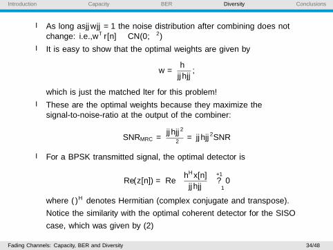
I As long as ||w|| = 1 the noise distribution after combining does notchange: i.e., wT r[n] ∼ CN(0, σ2)

I It is easy to show that the optimal weights are given by

w =h∗

||h|| ,

which is just the matched filter for this problem!

I These are the optimal weights because they maximize thesignal-to-noise-ratio at the output of the combiner:

SNRMRC =||h||2

σ2= ||h||2SNR

I For a BPSK transmitted signal, the optimal detector is

Re(z[n]) = Re

(hHx[n]

||h||

)+1

≷−1

0

where (·)H denotes Hermitian (complex conjugate and transpose).

Notice the similarity with the optimal coherent detector for the SISO

case, which was given by (2)



I Similarly to the SISO case, the Pe can be derived exactly

Pe = Q(√

2||h||2SNR),

which is a random variable because h is random (fading channel)

I Under Rayleigh fading, each hi is i.i.d CN(0, 1) and

x = ||h||2 =N∑i=1

|hi |2

follows a Chi-square distribution with 2N degrees of freedom

f (x) =1

(N − 1)!xN−1 exp(−x), x ≥ 0

I Note that the exponential distribution (SISO case with N = 1) is a

Chi-square with 2 degrees of freedom

I The average error probability can be explicitly computed, here we onlyprovide a high-SNR approximation

Pe =

∫ ∞0

Q(√

2xSNR)f (x)dx ≈

(2N − 1

N

)1

(4SNR)N



The probability of being in a deep fade with MRC is

Pr(||h||2SNR < 1) =

∫ 1/SNR

0

1

(N − 1)!xN−1 exp(−x)dx ≈

(for x small) ≈∫ 1/SNR

0

1

(N − 1)!xN−1dx =

1

N!SNRN

Conclusions

I The Pe is again dominated by the probability of being in adeep fade

I Both (the Pe and the probability of being in a deep fade)decrease with the number of antennas roughly as (SNR)−N

I MRC extracts all spatial diversity of the SIMO channel !!

However, MRC is not the only multiantenna technique thatextracts all spatial diversity of a SIMO channel



Antenna selection

1h

2h

Nh

][][][ max nrnshnx

1r

2r

Nr

RF chain

Selection of the best link

ADC

I In antenna selection the path with the highest SNR is selected andprocessed: x [n] = hmaxs[n] + r [n], where

hmax = max (|h1|, |h2|, . . . , |hN |)

I In comparison to MRC, only a single RF chain is needed !!



I Intuitively, the probability that the best channel is in a deepfade is

Pr(|hmax |2SNR < 1) =N∏i=1

Pr((|hi |2SNR < 1) ≈ 1

SNRN

and, therefore, the diversity of antenna selection is also N

I The same conclusion can be reached by studying the Pe (wewould need the distribution of |hmax |2)

I However, the output SNR of MRC is higher than that ofantenna selection (AS)

SNRMRC =|h1|2σ2

+ . . .+|hN |2σ2

SNRAS =|hmax |2σ2



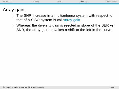
Array gainI The SNR increase in a multiantenna system with respect to

that of a SISO system is called array gain

I Whereas the diversity gain is reflected in slope of the BER vs.SNR, the array gain provokes a shift to the left in the curve

0 5 10 15 20 2510

−5

10−4

10−3

10−2

10−1

100

SNR (dB)

BE

R

N=1

N=2

Array Gain



I For a receiver with N antennas, MRC is optimal because itachieves maximum spatial diversity and maximum array gain

I MRC achieves the maximum array gain by coherentlycombining all signal paths

I On average, the output SNR of MRC is N times that of aSISO system, so its array gain is 10 log10 N (dBs)

I For instance, using 2 Rx antennas, MRC provides 3 extra dBsin comparison to a SISO system and in addition to the spatialdiversity gain



0 5 10 15 20 25

10−4

10−3

10−2

10−1

100

SNR (dB)

SER

Antenna Selection

N=2

N=3

MRC



Maximum Ratio TransmissionSimilar concepts apply for a a MISO (multiple-input single-input)channel: the optimal scheme is now called Maximum RatioTransmission (MRT)

1h

Nh

][nr

][][ ][ nrnsnz hwT

1w

2w

Nw

][ns 2h

Again, the optimal transmit beamformer that achieves full spatialdiversity (N) and full array gain (10 log10 N) is

w =h∗

||h|| ,

The main difference is that now the channel must be known at theTx (through a feedback channel)



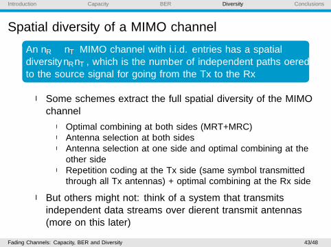
Spatial diversity of a MIMO channel

An nR × nT MIMO channel with i.i.d. entries has a spatialdiversity nRnT , which is the number of independent paths offeredto the source signal for going from the Tx to the Rx

I Some schemes extract the full spatial diversity of the MIMOchannel

I Optimal combining at both sides (MRT+MRC)I Antenna selection at both sidesI Antenna selection at one side and optimal combining at the

other sideI Repetition coding at the Tx side (same symbol transmitted

through all Tx antennas) + optimal combining at the Rx side

I But others might not: think of a system that transmitsindependent data streams over different transmit antennas(more on this later)



Time and frequency diversityI We have mainly focused the discussion on the spatial diversity

concept, but the same idea can be applied to the time andfrequency domains

I Time diversity:

1. The same symbol is transmitted over different time instants, t1

and t2

2. For the channel to fade more or less independently:|t1 − t2| > Tc = 1

Ds

I Frequency diversity:

1. The same symbol is transmitted over different frequencies(subcarriers in OFDM), f1 and f2

2. For the channel to fade more or less independently:|f1 − f2| > Bc = 1

τrms

I To achieve time or frequency diversity, interleaving istypically used



Interleaving

I The symbols or coded bits are dispersed over differentcoherence intervals (in time or frequency)

I A typical interleaver consists of an P × Q matrix: the inputsignals are written rowwise into the matrix and then readcolumnwise and transmitted (after modulation)

I Example: A 4× 8 interleaving matrix

3231302928272625

2423222120191817

161514131211109

87654321

ssssssssssssssssssssssssssssssss

323130292854321 ssssssssss 3224168312251791 ssssssssss

from source to channel



1h 2h

3231302928272625

2423222120191817

161514131211109

87654321

ssssssssssssssssssssssssssssssss

4321 ssss 8765 ssss 1211109 ssss3h

burst of errors

Without interleaving

1h 2h

251791 ssss 2618102 ssss 2719113 ssss3h

With interleaving

4h

16151413 ssss

4h

2820124 ssss



Remarks:

I Doppler spreads in typical systems range from 1 to 100 Hz,corresponding roughly to coherence times from 0.01 to 1 sec.

I If transmissions rates range from 2.104 to 2.106 bps, thiswould imply that blocks of length L ranging fromL = 2.104 × 0.01 = 200 bits to L = 2.106 × 1 = 2.106 bitswould be affected by approximately the same fading gain

I Deep interleaving might be needed in some cases

I But notice that interleaving involves a delay proportional tothe size of the interleaving matrix

I In delay-constrained systems (transmission of real-timespeech) this might be difficult or even unfeasible



Conclusions

I We have analyzed the effect of fading from the point of viewof capacity (only CSIR) and BER

I Depending of the channel model (ergodic or block fading) weuse ergodic capacity or outage capacity

I With CSIR only, the capacity of a fading channel is always lessthan the capacity of an AWGN with the same average SNR

I The effect of fading is more significant in terms of BER thanin terms of capacity (power of coding gain + interleaving)

I Diversity: slope of the BER wrt SNR at high SNRs

I Diversity techniques with multiantenna systems: MRT, MRC,antenna selection, etc

I We can extract the time and frequency diversity of thechannel through interleaving


Documents

Fading Channels: Capacity, BER and Diversity - … · I Fading channels: The instantaneous ... 1.Shannon’s coding theorem proves that a code exists that ... Fading Channels: Capacity,