Factors affecting the quality of XBT data? results of

HAL Id: hal-00298314https://hal.archives-ouvertes.fr/hal-00298314

Submitted on 8 Feb 2007

HAL is a multi-disciplinary open accessarchive for the deposit and dissemination of sci-entific research documents, whether they are pub-lished or not. The documents may come fromteaching and research institutions in France orabroad, or from public or private research centers.

L’archive ouverte pluridisciplinaire HAL, estdestinée au dépôt et à la diffusion de documentsscientifiques de niveau recherche, publiés ou non,émanant des établissements d’enseignement et derecherche français ou étrangers, des laboratoirespublics ou privés.

Factors affecting the quality of XBT data ? results ofanalyses on profiles from the Western Mediterranean Sea

F. Reseghetti, M. Borghini, G. M. R. Manzella

To cite this version:F. Reseghetti, M. Borghini, G. M. R. Manzella. Factors affecting the quality of XBT data ? resultsof analyses on profiles from the Western Mediterranean Sea. Ocean Science, European GeosciencesUnion, 2007, 3 (1), pp.59-75. �hal-00298314�

https://hal.archives-ouvertes.fr/hal-00298314

https://hal.archives-ouvertes.fr

Ocean Sci., 3, 59–75, 2007www.ocean-sci.net/3/59/2007/© Author(s) 2007. This work is licensedunder a Creative Commons License.

Ocean Science

Factors affecting the quality of XBT data – results of analyses onprofiles from the Western Mediterranean Sea

F. Reseghetti1, M. Borghini 2, and G. M. R. Manzella3

1ENEA-ACS-CLIM-MED, Forte S. Teresa – Pozzuolo di Lerici, 19032 Lerici (Sp), Italia2CNR-ISMAR, Sez. Oceanografia Fisica, Forte S. Teresa – Pozzuolo di Lerici, 19032 Lerici (Sp), Italia3ENEA-ACS, Forte S. Teresa – Pozzuolo di Lerici, 19032 Lerici (Sp), Italia

Received: 5 May 2006 – Published in Ocean Sci. Discuss.: 1 September 2006Revised: 29 November 2006 – Accepted: 2 February 2007 – Published: 8 February 2007

Abstract. EXpendable BathyThermograph (XBT) temper-ature profiles collected in the framework of the Mediter-ranean Forecasting System – Toward Environmental Pre-diction (MFS-TEP) project have been compared with CTDmeasurements. New procedures for the quality control ofrecorded values have been developed and checked. Somesources of possible uncertainties and errors, such as the re-sponse time of the apparatus (XBT probe, thermistor andreadout chain), or the influence of initial conditions are alsoanalysed. To deal with the high homogeneity of Mediter-ranean waters, a new technique to compute the fall rate coef-ficients, that give a better reproduction of the depth of ther-mal structures, has been proposed, and new customized co-efficients have been calculated. After the application of atemperature correction, the overall uncertainties in depth andin temperature measurements have been estimated.

1 Introduction

Since the 60’s, XBT probes have been successfully adoptedby oceanographers as an easy way to collect temperature pro-files by using commercial ships (Ship Of Opportunity Pro-grams – SOOP). Different types of probes are available: T4,T5, T6, T7, Deep Blue (DB), Fast Deep (FD) etc., and theircharacteristics are reviewed in several “Cookbooks”, e.g. Sy(1991), AODC (1999, 2001 and 2002), Cook and Sy (2001).The choice of the type depends on ship speed and on ter-minal depth. In Table 1, some properties based on guidesproduced by the manufacturer (Lockheed Martin Sippican –USA, hereafter Sippican) are detailed. Several analyses onthe quality of XBT temperature profiles have been published,and a lot of influencing factors have been identified (Seaver

Correspondence to: F. Reseghetti([email protected])

and Kuleshov, 1982; Green, 1984; Singer, 1990; Hallock andTeague, 1992).

The main problems are the evaluation of the uncer-tainty in recorded temperature values and the estimate ofthe depth, which is calculated through a fall rate equationZ(t)=At−Bt2, whereZ is the depth at the timet . The coef-ficients are both positive and depend on XBT types (Table 2).

“A” is related to the hydrodynamics characteristics of theprobe, and is equivalent to the initial falling speed, “B” isa function of the mass variation rate of the probe, and of thevariation of seawater properties depending on the depth, suchas density and viscosity (e.g. Seaver and Kuleshov, 1982;Green, 1984; Hanawa et al., 1994, 1995).

Since the end of the 70’s, some inadequacies were recog-nised between the computed depths and the values measuredby other oceanographic instruments, such as STD or CTD(e.g. McDowell, 1977; Flierl and Robinson, 1977; Fedorovet al., 1978). In 1994, the Integrated Global Ocean ServicesSystem (IGOSS) Task Team released a comprehensive re-port on XBT/CTD comparison and proposed a new compu-tational technique (Hanawa et al., 1994, 1995), derived fromthe approach implemented by Hanawa and Yasuda (1992).New values for fall rate coefficients for T4/T6/T7/DB probesmanufactured by Sippican and TSK (Tsurumi Seiki Co. –Japan) were calculated (see Table 2). The best-fit values forT4/T6 and T7/DB probes are not coincident: such a smalldiscrepancy, even if within the standard deviation, could indi-cate that the probe motion slightly depends on the XBT type.The error in the depth value was estimated to be 2% of thedepth or 5 m, whichever is greater. In spite of the consensuson the IGOSS fall rate coefficients, which were calculatedby using data from the major world oceans (but not from theMediterranean Sea), discrepancies were found in some areas,such as in the Antarctic Ocean (Thadathil et al., 2002).

Analyses of XBT performances in the Mediterranean Seaare not available: it was noted that XBT profiles from theLigurian Sea have a general agreement with CTD profiles,

Published by Copernicus GmbH on behalf of the European Geosciences Union.

60 F. Reseghetti et al.: XBT quality procedures in the Mediterranean

Table 1. Some characteristics of different XBT probes. Nominal maximum speed and experimental range of speed are shown in the first twocolumns; then, the terminal depth and the correspondent nominal acquisition time AT (as deduced by using IGOSS fall rate coefficients). Ifthe fall rate coefficients proposed by manufacturer are used, the acquisition time for T4/T6 probes is 72.9 s, and 122.5 s for T7/DB probes.The averaged acquisition time (<AT>) and the correspondent depth calculated following the procedure detailed in Manzella et al. (2003),with the measured range, are quoted. Values concerning T4 and DB probes atv ≥20 kn are based on XBTs dropped on the transect Genova-Palermo. The number of XBT probes in each dataset is added.

XBT Type Max Speed Real Speed Depth AT <AT> Range Average Depth Range No. XBT(kn) (kn) (m) (s) (s) (s) (m) (m)

T4 30 0 460 70.5 87.3±2.0 83.0–90.7 567±12 540–588 22T4 30 21–27 460 70.5 80.6±1.1 76.8–84.9 525±7 500-552 230T6 15 ≤10 460 70.5 85.2±4.1 77.7–90.5 554±26 506–587 11T5 6 4–6 1830 290.5 352.9±9.7 332.9–362.9 2183±54 2071–2238 14T7 15 ≤15 760 118.3 142.5±2.2 138.6–150.9 908±14 884–958 68T7 15 17 760 118.3 136.3±1.4 133.2–138.2 870±9 851–881 15DB 20 0 760 118.3 143.9±2.4 139.3–148.5 916±14 888–944 18DB 20 ≤20 760 118.3 140.9±1.8 126.3–149.6 898±11 809–951 1312DB 20 21 760 118.3 137.6±1.9 136.3–140.5 878±12 870–896 4DB 20 22 760 118.3 134.2±2.2 130.9–140.3 857±13 837–894 27DB 20 23 760 118.3 127.5±2.3 124.3–132.8 817±14 797–849 35DB 20 24 760 118.3 122.1±2.9 115.6–127.0 783±18 743–813 31DB 20 25 760 118.3 118.0±2.3 113.0–123.8 758±14 727–794 48DB 20 26 760 118.3 114.2±2.5 109.3–118.6 735±15 704–762 37DB 20 27 760 118.3 111.1±1.2 109.8–113.5 716±8 707–730 9

Table 2. Different values for the coefficients of the fall rate equa-tion are compared. IOC proposed Hanawa et al. (1995) values forT4, T6, T7 and DB as official IGOSS fall rate coefficients for suchprobes. The values obtained from the best fit for specific XBT typesare added.

Author A (ms−1) B (ms−2)

Sippican T4/T6/T7/DB 6.472 0.00216Sippican T5 6.828 0.00182Sippican FD 6.390 0.00182Hanawa et al. (1995) 6.691±0.021 0.00225±0.00030T4/T6/T7/DBHanawa et al. (1995) 6.683±0.033 0.00215±0.00052Best fit T4/T6Hanawa et al. (1995) 6.701±0.023 0.00238±0.00016Best fit T7/DB

but some discrepancies occur at the thermocline depth andin correspondence with deep thermal structures (Reseghetti,20031). Consequently, the acquisition of several pairs of co-located and contemporaneous XBT/CTD temperature pro-files in the Western Mediterranean Sea was planned within

1Reseghetti, F.: Comparison between quasi contemporaneousand co-located CTD and XBT measurements, MFS-TEP – VOSTechnical Report Nr. 1 (unpublished) available at: http://moon.santateresa.enea.it/documents/xbtvsctd.pdf, 2003.

the Mediterranean Forecasting System – Toward Environ-mental Prediction (MFS-TEP) project, in order to evaluateXBT performance and to improve experimental proceduresand data processing. Thermal structures and their depth havebeen identified on recorded XBT and CTD temperature pro-files, whereas the correspondentdT /dz profiles have offeredthe opportunity to estimate the capability of the XBT probesin measuring thermal variation. Then, temperature differ-ence profiles (1T =T (XBT)−T (CTD)) have shown the de-pendence of discrepancy on depth.

New fall rate coefficients and data analysis procedures,that reproduce better the depth of thermal structures, and anew estimate of the temperature uncertainty have been de-termined. This paper summarizes the results of the activitydeveloped within MFS-TEP and ADRICOSM (ADRIatic seaintegrated COastal areas and river basin Management systempilot project), and is organised as follows: in Sect. 2, XBTand CTD data collection procedures are presented; in Sect. 3,data analysis, including the evaluation of factors influencingthe motion of the probe, the quality of measurements andnew fall rate coefficients are reviewed; in Sect. 4, the valuesof the uncertainty in temperature are detailed; comments andfinal remarks are in Sect. 5.

Ocean Sci., 3, 59–75, 2007 www.ocean-sci.net/3/59/2007/

http://moon.santateresa.enea.it/documents/xbtvsctd.pdf

http://moon.santateresa.enea.it/documents/xbtvsctd.pdf

F. Reseghetti et al.: XBT quality procedures in the Mediterranean 61

2 Materials and methods

In this paper, the speed of a ship is in knots (kn), and XBTtemperatures are in situ values in Celsius degrees (◦C). CTDprofiles are considered the “true” representation of the tem-perature: the differences between CTD and XBT values areassumed to reflect inaccuracies in the XBT measurements,which are released with three decimal digits, due to the math-ematical processing.

2.1 CTD characteristics and its data processing

CTD profiles were recorded using a Sea-Bird SBE 911plusautomatic profiler, calibrated before and after each cruiseat NURC (NATO Undersea Research Centre, La Spezia –Italia). The adopted falling speed was 1.0 ms−1. The ap-paratus has a 24 Hz sampling rate, with a (static) nominalaccuracy of 0.001◦C in temperature, and of 0.0003 Sm−1 inconductivity. The (static) time constants are 0.065 s for theconductivity and temperature sensors (which implies a nomi-nal spatial resolution of 0.065 m), and 0.015 s for the pressuresensor (the spatial resolution is 0.015 m). CTD profiles wereprocessed using standard Seabird’s software (Data Conver-sion, Alignment, Cell Thermal Mass, Filtering, Derivationof physical values, Bin Average and Splitting); afterwards,they were qualified with Medatlas protocols (Maillard andFichaut, 2001).

2.2 XBT data acquisition and data processing

Some types of XBT probes manufactured by Sippican in dif-ferent years were launched during CTD casts from the CNR’sR/V URANIA when the ship was motionless. Different sea-water characteristics were found: a weak surface thermoclinein May 2003 and in May 2004, a strongly stratified upperlayer (down to about 100 m depth) in September 2003 andSeptember–October 2004, and winter-homogenised watersin January 2004. Geographical and temporal co-ordinates foreach pair of CTD cast and XBT probe are shown in Fig. 1.Specific analyses and results are concerned with the T4 andDB probes, but a significant part of the conclusions can beextended either to T6 or to T7 probes. The physical proper-ties of T4/T6 and T7/DB pairs of probes are the same, withinthe probe-to-probe variability, with the length of copper wireon the shipside as the only known difference between T4 andT6, or T7 and DB probes. The data acquisition system con-sists of Sippican MK-12 readout card, PC with Intel P-II 166MHz-processor. The XBT sampling rate is 10 Hz, the in-strumental sensitivity on temperature is 0.01◦C, whereas theuncertainty estimated by the manufacturer is|δT |∼0.10◦C.Each XBT probe was dropped within 480 s from the start ofa CTD cast.

Fig. 1. The position of 55 XBT probes launched close to the corre-sponding CTD cast is shown: the mean difference was 0.0002◦ bothin latitude and in longitude, with a time delay ranging from 60 upto 480 s (the mean value was 180 s). The averaged delay time was180 s (ranging from 60 up to 480 s). The usual height of the launch-ing position was 2.5 m a.s.l., with the exception of five T4 and sixDB probes dropped from 8 m a.s.l. (superimposed symbols).

3 Data analysis

3.1 Extended use below the nominal terminal depth and ac-quisition time

Since April 2003, data acquisition beyond the nominal ter-minal depth has been the standard procedure for XBT probesdropped within MFS-TEP and ADRICOSM. In such a way,most of the copper wire on the probe side is used, and tem-perature values are recorded at depths greater than nominal.Practically, the depth in the Sippican software is set to 600 mfor T4/T6 probes, to 900 or 1000 m for T7/DB probes, and to2500 m for T5 probes. The Sippican MK-12 Electronic Helpadmits such a procedure, but a terminal depth increased byno more than 20% is recommended.

The data acquisition has been estimated as “valid” untilsharp variations toward negative values are recorded (usually−2.5◦C), indicating that the copper wire breaks on shipside,or high values are detected (about 36◦C), implying a wirebreak on probe-side.

The comparison between XBT and contemporaneous andco-located CTD profiles does not show unusual features inthe recorded values. T4 probes have measured tempera-

www.ocean-sci.net/3/59/2007/ Ocean Sci., 3, 59–75, 2007


Fig. 2. Temperature difference (T (XBT)−T (CTD)) in deeper part of each XBT profiles: in(a) for 28 T4 probes below 300 m depth, in(b)for 27 DB probes below 600 m depth. The depth is computed by using IGOSS coefficients and data processing described in Manzella etal. (2003). The black dashed line indicates the nominal terminal depth. The plots have different scales.

tures higher than the corresponding CTD (Fig. 2a): only oneprofile always has values consistently lower, and four pro-files have significant spikes corresponding to thermal struc-tures. The range of temperature differences below the nomi-nal terminal depth is−0.03◦C≤1T ≤+0.16◦C. On the otherhand, DB probes have always recorded temperatures higherthan the corresponding CTD, and four profiles show evidentspikes (Fig. 2b); their range of variability below their nomi-nal terminal depth is−0.02◦C≤1T ≤+0.12◦C.

The depth of a probe at a selected time is estimatedthrough a fall rate equation, but the true free parameter is theacquisition time (AT), the temperature values being recordedat a fixed rate. The maximum value of the acquisition timedepends on the XBT type: it is calculated by dividing thenumber of rows in the acquisition file by the sampling rate of10 Hz. In Table 1, AT values corresponding to the nominalterminal depth are shown. AT values lower than the nominalone (mainly due to spikes or failed launches) were not in-cluded in the statistics, as well as in the case of profiles with-out a signal clearly indicating that acquisition was stopped.Several probes dropped in extended mode within MFS-TEPand ADRICOSM projects continued their data acquisition upto the selected end, even after the probe touched the bottom.If a XBT probe is dropped from a steady vessel, its AT val-ues can be assumed to be nearly coincident with the maxi-mum value (e.g. about 90 s for T4/T6, and 150 s for T7/DBprobes). Analyses of XBT probes launched within MFS-TEPand ADRICOSM confirm that such values are more or lessconstant when the ship speedv is smaller than 19 kn for T4and smaller than 16 kn for DB probes, and, as expected, theydecrease at higher speed (Table 1). As an example, the fre-quency distribution of the acquisition time values is shown

in Fig. 3a for T4 probes, and in Fig. 3b for DB probes. Inthis case, the distribution is practically Gaussian around theexperimental mean value.

For XBT probes dropped from ships moving faster thanthe maximum value indicated by the manufacturer, AT valuessmaller than the nominal ones should be expected, and ex-perimental results agree with this assumption. The mean ATvalues for 191 DB probes launched from May 2004 to De-cember 2005 along the transect Genova-Palermo from shipsmoving at speedv>20 kn are detailed in Table 1. Temper-ature values recorded by DB probes do not show evidentanomalies depending on the ship speed.

The dataset of T7 probes within MFS-TEP and ADRI-COSM is small: 68 probes were launched from ships movingat v≤15 kn, and 15 probes from ships moving atv∼17 kn.Their AT values are as great as the ones of DB probes (Ta-ble 1).

Only 14 T5 probes were dropped with extended acquisi-tion: as for the other XBT types, their AT values are about20% higher than the nominal one (Table 1).

3.2 Factors influencing the XBT motion

3.2.1 Launching position height

The acquisition of good data in the near surface layer isstrongly dependent on events occurring during the first sec-onds after the probe touches seawater: therefore, the launch-ing procedures (including the height (H ) of the launchingpoint above the sea level, and the verticality of the probewhen it goes into the seawater), are briefly analysed. In theworking procedures, it is fundamental to make sure that theprobe quickly reaches a spin rate of about 15 Hz in seawater,



Fig. 3. Frequency distribution of acquisition time (AT) for different type of probes. In(a), values for T4 probes launched within MFS-TEPalong the transect Genova-Palermo from May 2004 to December 2005, at a ship speed ranging from 21 to 27 kn, are shown. In(b), valuesfor DB probes dropped in the same period atv≤20 kn. Some counts at AT=141.3 s are due to probes dropped by setting the terminal depthto 900 m in software.

a value needed to maintain the vertical direction of the mo-tion through the water and the standard falling conditions.Analyses performed by Hallock and Teague (1992) showedthat T4/T6/T7/DB probes require more or less 1.5 s to reacha falling speed of about 6.5 ms−1, independent of the entryspeed.

The manufacturer recommendsH∼2.5 m a.s.l.: if exter-nal causes do not modify the fall, the entry speed when theprobe touches seawater is about 6.5 ms−1, as great as theAcoefficient in the fall rate equation. A much higher launch-ing height increases the entry speed, and the depth computedby software could be wrong. It is also important that theprobes touch the seawater in the vertical position, otherwisethe initial falling velocity within seawater could be smallerthan 6.5 ms−1. In this case, the actual XBT depth would besmaller than the one computed by software. The number ofslant impacts could increase when the ship moves faster orthe wind is stronger, but the evaluation of what really hap-pens is unpredictable. Usually, the depth discrepancy canbe identified in the region where a thermal gradient starts.Non-standard launching conditions should be described byan offset term (smaller than 5 m) added to the depth com-puted by applying the usual fall rate equation. Before theanalyses made by Hanawa et al. (1994, 1995), this was thesolution proposed in some papers in order to calculate betterthe XBT depth (i.e. Singer, 1990).

Differences between the theoretical (i.e. computed by us-ing the fall rate equation), and the real estimated depthsD

(1D=D(estim)−D(theor)) were obtained by Green (1984),who analysed the influence of the launching position height(i.e. the entry speed). He found depth values greater thanthe nominal ones: his correction varies from1D∼1.1 m (ifH∼8.5 m) to1D∼1.9 m (if H∼20 m).

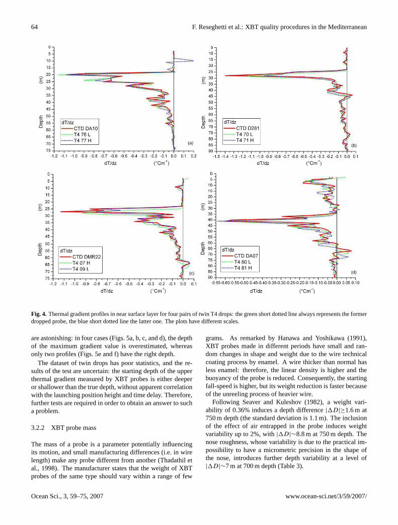
In September–October 2004, twin XBT drops were madeduring the same CTD cast from different positions (H∼2.5 mandH∼8.0 m, respectively), aiming to check the influenceof the launching position height, namely the depth differencepredicted by Green (1984). The strong seasonal thermoclinehas offered a good reference feature for the test; in addition,the launching conditions have been optimal: ship motionless,good weather and sea status. The time delay between the pairof drops and the CTD cast was smaller than 480 s, i.e. thevariation of the depth of upper thermocline should have beenvery small. In all twin T4 profiles, such thermal structure isgenerally well reproduced both in depth and in intensity, in-dependent of the time-delay and the height of the launchingposition (see Fig. 4, where the temperature gradient profilesare shown). Sometimes, discrepancies appear below this re-gion (observed depths greater than CTD values), indicatingsome variation in the probe motion (Fig. 4d).

Results are significantly different for DB probes: in gen-eral, their profiles reproduce well the intensity of the upperthermal gradient, but not the depth. Only one pair of DB twindrops has both profiles fitting the CTD profile in an excellentway (Fig. 5e). In four cases (Figs. 5a, b, c, and f), the lastdropped probe overestimates the depth of the maximum gra-dient value, whereas only one probe (Fig. 5d) underestimatessuch a value. In general, the first dropped probe has a smallerdiscrepancy, with only one significant difference (Fig. 5c).

When the height of launching position is considered, theprobes dropped atH∼8 m a.s.l. fit well the depth of max-imum gradient in three cases (Figs. 5a, b, and e); in twocases, the XBT profiles underestimate the true depth (Figs. 5cand d), whereas the only case with an overestimated depth isshown in Fig. 5f. In a certain way, results for DB probesdropped atH∼2.5 m (as recommended by the manufacturer)



Fig. 4. Thermal gradient profiles in near surface layer for four pairs of twin T4 drops: the green short dotted line always represents the formerdropped probe, the blue short dotted line the latter one. The plots have different scales.

are astonishing: in four cases (Figs. 5a, b, c, and d), the depthof the maximum gradient value is overestimated, whereasonly two profiles (Figs. 5e and f) have the right depth.

The dataset of twin drops has poor statistics, and the re-sults of the test are uncertain: the starting depth of the upperthermal gradient measured by XBT probes is either deeperor shallower than the true depth, without apparent correlationwith the launching position height and time delay. Therefore,further tests are required in order to obtain an answer to sucha problem.

3.2.2 XBT probe mass

The mass of a probe is a parameter potentially influencingits motion, and small manufacturing differences (i.e. in wirelength) make any probe different from another (Thadathil etal., 1998). The manufacturer states that the weight of XBTprobes of the same type should vary within a range of few

grams. As remarked by Hanawa and Yoshikawa (1991),XBT probes made in different periods have small and ran-dom changes in shape and weight due to the wire technicalcoating process by enamel. A wire thicker than normal hasless enamel: therefore, the linear density is higher and thebuoyancy of the probe is reduced. Consequently, the startingfall-speed is higher, but its weight reduction is faster becauseof the unreeling process of heavier wire.

Following Seaver and Kuleshov (1982), a weight vari-ability of 0.36% induces a depth difference|1D|≥1.6 m at750 m depth (the standard deviation is 1.1 m). The inclusionof the effect of air entrapped in the probe induces weightvariability up to 2%, with|1D|∼8.8 m at 750 m depth. Thenose roughness, whose variability is due to the practical im-possibility to have a micrometric precision in the shape ofthe nose, introduces further depth variability at a level of|1D|∼7 m at 700 m depth (Table 3).



Fig. 5. As in Fig. 4, for all the pairs of twin DB drops. The plots have different scales.



Table 3. Effects induced on the values of fall rate coefficients and computed depth quoted by different authors for T7/DB probes (see thetext for details). Depth values quoted in (*) are from Seaver and Kuleshov (1982).

Source of Uncertainty Depth m Variation onA (ms−1) Variation onB (ms−2)

Horizontal Current −0.7 −0.005 −0.00003v=0.25 ms−1

Weight variability* ±8.8 ±0.013 ±0.00007Nose roughness* ±7.0 ±0.063 ±0.00055

In order to identify a possible correlation between weightand acquisition time, the mass (in air) of some boxes of DBprobes was measured. In detail, each probe within the can-ister (but without the cap) was weighed before the drop, andthe components of the canister were again weighed after thelaunch. In addition, the components of some probes wereweighed, and the length of their copper wire was measured.When different boxes are compared, the mean weight of thewhole probe and plastic canister (averaged on 12 probes) ismore or less constant, with the standard deviation (4 g), butthe probe-to-probe variability within a box is high (up to 15 g,about 1.5% of the weight). The range of variability of retain-ing pin and shipboard plastic spool is small, but large forthe plastic canister, probably due to the quantity and char-acteristics of the insulating wax. From the comparison ofthe weight of the components, the range of weight variabil-ity of the naked probes is 5 g (more or less as the manufac-turer states), but any estimate of its influence on the motionin seawater (mainly on the fall rate coefficients) is impossi-ble. The weight of the zinc nose is constant for both T4 andDB XBT types, within 1 g variability. Therefore, 4 g is themore probable weight variability for the plastic and the wirecomponent of a probe. The measured linear density of cop-per wire varies between 0.116 and 0.121 gm−1, independentof the XBT type, or, in other words, one gram of wire cor-responds to about 8.5 m. This means that the variability dueto the uncertainty in the probe weight is up to about 35 m (ormore than 5 s in acquisition time).

3.2.3 Other sources of uncertainties

A constant horizontal current havingv=0.25 ms−1 has beenconsidered from the theoretical point of view: it can shift theprobe from the vertical fall up to 22 m for T4/T6 probe (at550 m depth), and to 35 m for DB (at 900 m depth). Conse-quently, the real depth is smaller than the computed one. Theestimated effect of such terms on fall rate coefficients for DBprobes is reviewed in Table 3.

3.3 Start-up transient

The time response of the recording system can influence thequality of XBT measurements mainly in upper layers, wherequick thermal changes occur. The thermistor has a time con-

stant (TC) of 0.15 s: this is the time required to detect the63% of a step thermal signal, whereas the overall time con-stant (OTC), which describes the response time of the wholeacquisition system, is slightly greater (OTC∼0.16 s). Dur-ing such a time interval, the probe falls about 1 m and this isthe depth uncertainty intrinsic to the acquisition system. Thebridge circuit reaches equilibrium within two sampling in-tervals (the thermistor output is sampled at a constant rateof 10 Hz), but an interval as great as 4.5 TC (about 0.6–0.7 s) might be needed before the probe completely detectsa temperature variation. In addition, the probe nose and theread-out card might influence the initial transient time up toabout 0.1 s (Roemmich and Cornuelle, 1987). Consequently,it seems realistic to suppose that the true water temperaturein near surface layers can be detected below about 4 m depth(or 0.5 s in acquisition time). It has to be pointed out thatStegen et al. (1975) eliminated values from the surface downto 4 m depth, Kizu and Hanawa (2002a) proposed a cut vary-ing from 2 to 10 m, depending on the readout card, whereasManzella et al. (2003) excluded temperature values from sur-face down to 5 m.

In this work, the first ten recorded temperature values of allthe available profiles have been analysed in order to calculatethe Empirical Time Constant (ETC), which is defined as thetime needed before the probes reach the stationary regimein seawater. It is identified by the occurrence of three con-secutive temperature values differing less than 0.10◦C (thenominal accuracy) within the first ten measurements. Themean value of such time intervals for all the probes of a se-lected type is the mean response time (ETC) for that XBTtype. The value obtained for both T4 and DB probes isETC=0.3±0.1 s (twice the overall time constant of the acqui-sition system). Then, the sequence of temperature values ofeach XBT profile has been modified by eliminating the val-ues recorded up to timet=ETC, and the measurement at thetime t=ETC+0.1 s has been considered as the first one. Thefirst three temperature values have been eliminated from eachXBT profile, and the fourth recorded value is the first validvalue. This implies a 2 m correction to the whole profile.

After the application of this procedure, the discrepanciesbetween XBT and CTD temperature values in upper layersare significantly reduced (Fig. 6a for T4 and Fig. 6b for DBprobes). The mean temperature difference profile is more



Fig. 6. Comparison between mean temperature difference (with one standard deviation) with data processing as in Manzella et al. (2003), inred, and after the application of ETC correction, in blue: in(a) T4 probes, and in(b) DB probes. The plots have different scales.

symmetric with respect to the null value, and the initial posi-tion of thermal structures in upper regions is reproduced bet-ter for both XBT types. In any case, this empirical proceduredoes not provide any understanding of phenomena related tothe correction.

3.4 Calibration of XBT probes and data acquisition system

Several authors have detected discrepancies between theXBT values and selected reference temperatures either insitu (Heinmiller et al., 1983) or in a calibration bath: al-ways T (XBT)≥T (CTD). Since the early 80’s, it has beensuggested that the calibration of XBT probes could provideindications of the source of errors (Georgi et al., 1980), andthe variability in temperature differences has been attributedto the probe-to-probe variability, e.g. Georgi et al. (1979,1980), Roemmich and Cornuelle (1987), and Budeus andKrause (1993).

Seaver and Kuleshov (1982) found a difference of 0.025◦C(0.015◦C in a controlled and digitised interface), which wasascribed to temperature-resistance characteristics of the ther-mistor. Such a temperature difference is equivalent to a deptherror varying from a few metres (in the upper warm layer) upto 20 m (at the bottom). Roemmich and Cornuelle (1987)measured a difference of 0.02–0.03◦C, and identified a smallpressure effect on the thermistor (about 0.01◦C/1000 m) dueto the non-standard quality of the production of the probecomponents.

In the middle of the 90’s, several hundreds of T4 andT7 probes were calibrated at NURC Laboratories. The se-lected reference temperatures wereT =12◦C, andT =22◦C:systematically, XBTs indicated temperatures higher than the

bath (Zanasca, 19962; private communication, 2005). For T4probes, the overall difference was 0.02±0.02◦C at the lowertemperature and 0.03±0.03◦C at the higher one, whereasT7 probes showed a constant difference (0.02±0.04◦C). Theuse of various PCs and readout cards (of the same type)can also influence the results of measurements. When twodifferent data acquisition systems were connected with thesame XBT probe, a difference of 0.02±0.01◦C was mea-sured (Zanasca, 19962), whereas Kizu and Hanawa (2002b)obtained a much greater effect (up to 0.10◦C), depending onthe type of recording card.

In September 2004, six T4 and six DB probes were cali-brated at NURC Laboratories at four reference temperatures(12.5, 16, 20, and 24◦C). The data were recorded by alwaysusing the same acquisition system composed by a PC, Sip-pican MK-12 card, cable, and connection box. Each probewas immersed in the bath 10 min before the data acquisition,which was 30.0 s long. Such a procedure should allow theidentification of the intrinsic bias due to the thermistor andthe data acquisition system. For each probe the measuredtemperatures are always higher than the bath and increasingwith the temperature (from 0.04◦C to 0.08◦C), the standarddeviation being 0.01◦C at the lower temperature, and 0.03◦Cat higher values (Fig. 7a for T4 and Fig. 7b for DB probes).When compared with earlier calibrations made at NURC,new results indicate higher temperature differences, but thestandard deviation is smaller. On the other hand, similar tem-perature differences were confirmed by in situ measurements(MEDARGO floats), although most of them were not exactlycontemporaneous and co-located with XBT probes droppedduring MFS-TEP (Poulain, private communication, 2005).

2Zanasca, P.: NURC Internal Notes (unpublished), 1996.



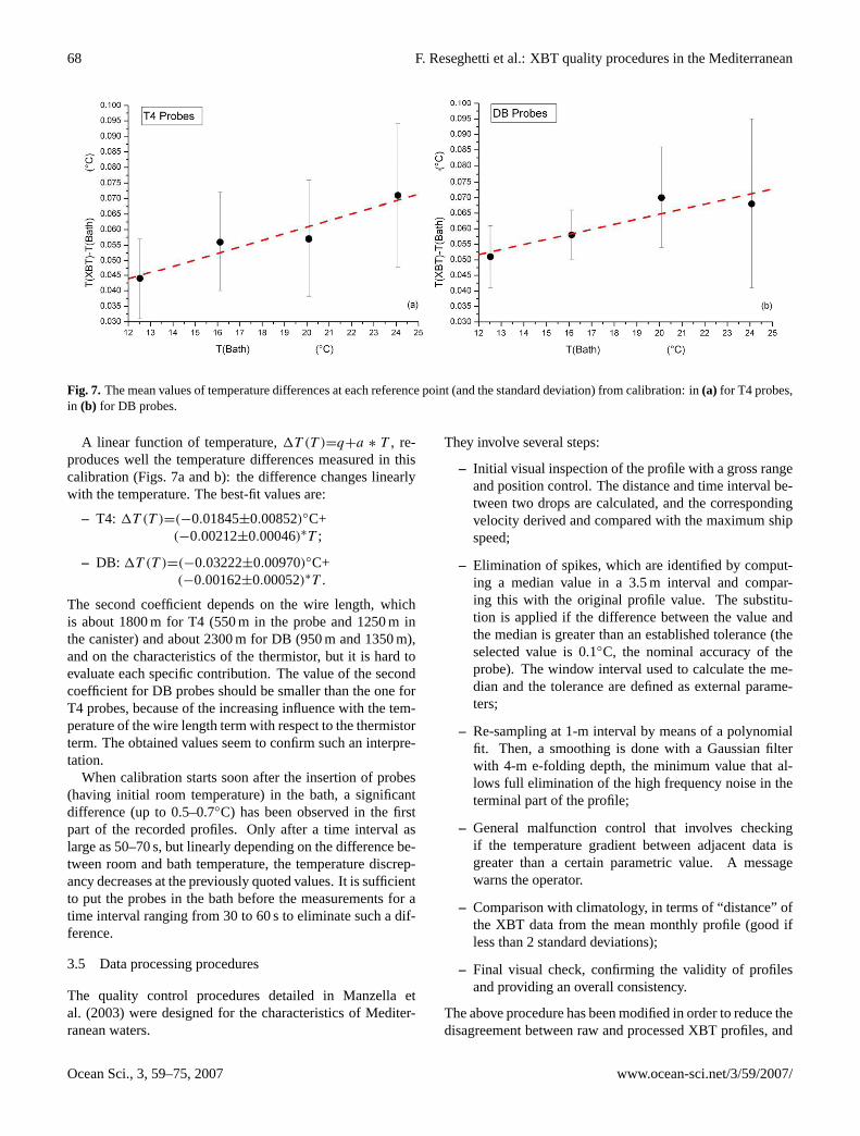
Fig. 7. The mean values of temperature differences at each reference point (and the standard deviation) from calibration: in(a) for T4 probes,in (b) for DB probes.

A linear function of temperature,1T (T )=q+a ∗ T , re-produces well the temperature differences measured in thiscalibration (Figs. 7a and b): the difference changes linearlywith the temperature. The best-fit values are:

– T4: 1T (T )=(−0.01845±0.00852)◦C+(−0.00212±0.00046)∗T ;

– DB: 1T (T )=(−0.03222±0.00970)◦C+(−0.00162±0.00052)∗T .

The second coefficient depends on the wire length, whichis about 1800 m for T4 (550 m in the probe and 1250 m inthe canister) and about 2300 m for DB (950 m and 1350 m),and on the characteristics of the thermistor, but it is hard toevaluate each specific contribution. The value of the secondcoefficient for DB probes should be smaller than the one forT4 probes, because of the increasing influence with the tem-perature of the wire length term with respect to the thermistorterm. The obtained values seem to confirm such an interpre-tation.

When calibration starts soon after the insertion of probes(having initial room temperature) in the bath, a significantdifference (up to 0.5–0.7◦C) has been observed in the firstpart of the recorded profiles. Only after a time interval aslarge as 50–70 s, but linearly depending on the difference be-tween room and bath temperature, the temperature discrep-ancy decreases at the previously quoted values. It is sufficientto put the probes in the bath before the measurements for atime interval ranging from 30 to 60 s to eliminate such a dif-ference.

3.5 Data processing procedures

The quality control procedures detailed in Manzella etal. (2003) were designed for the characteristics of Mediter-ranean waters.

They involve several steps:

– Initial visual inspection of the profile with a gross rangeand position control. The distance and time interval be-tween two drops are calculated, and the correspondingvelocity derived and compared with the maximum shipspeed;

– Elimination of spikes, which are identified by comput-ing a median value in a 3.5 m interval and compar-ing this with the original profile value. The substitu-tion is applied if the difference between the value andthe median is greater than an established tolerance (theselected value is 0.1◦C, the nominal accuracy of theprobe). The window interval used to calculate the me-dian and the tolerance are defined as external parame-ters;

– Re-sampling at 1-m interval by means of a polynomialfit. Then, a smoothing is done with a Gaussian filterwith 4-m e-folding depth, the minimum value that al-lows full elimination of the high frequency noise in theterminal part of the profile;

– General malfunction control that involves checkingif the temperature gradient between adjacent data isgreater than a certain parametric value. A messagewarns the operator.

– Comparison with climatology, in terms of “distance” ofthe XBT data from the mean monthly profile (good ifless than 2 standard deviations);

– Final visual check, confirming the validity of profilesand providing an overall consistency.

The above procedure has been modified in order to reduce thedisagreement between raw and processed XBT profiles, and



Fig. 8. Profiles of different thermal characteristics of a T4 probe and of the correspondent CTD cast: on the left column the range is 0–150 mdepth, on the right column the values below 150 m are plotted. In(a) and(b) the temperatures are shown: CTD (full black line), XBT withold data processing and IGOSS coefficients (dashed red line), XBT with new data processing and new fall rate coefficients (dotted green line),XBT with new data processing, new fall rate coefficients and temperature correction (short dotted blue line). In(c) and(d), the differenceT (XBT)−T (CTD) is plotted: XBT with old data processing and IGOSS coefficients (dashed red line), XBT with new data processing andnew fall rate coefficients without temperature correction (dotted green line), XBT with new data processing, new fall rate coefficients andtemperature correction (short dotted blue line). In(e)and(f), dT /dz values are shown, where the lines and the colours are the same as in (a)and (b). The plots have different scales and units.



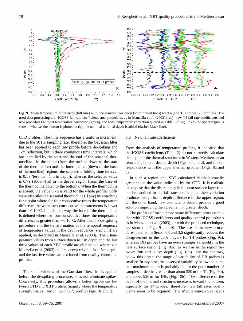
Fig. 9. Mean temperature differences (full line) with one standard deviation (short dotted lines) for T4 (and T6) probes (28 profiles). Theused data processing are: IGOSS fall rate coefficients and procedures as in Manzella et al. (2003) (red); new T4 fall rate coefficients andnew procedures without temperature correction (green), and with temperature correction quoted in Table 5 (blue). In(a) the upper region isshown, whereas the bottom is plotted in(b); the nominal terminal depth is added (dashed black line).

CTD profiles. The time sequence has a uniform increment,due to the 10 Hz sampling rate: therefore, the Gaussian filterhas been applied to each raw profile before de-spiking and1-m reduction, but in three contiguous time intervals, whichare identified by the start and the end of the seasonal ther-mocline. In the upper (from the surface down to the startof the thermocline) and the intermediate (down to the baseof thermocline) regions, the selected e-folding time intervalis 0.1 s (less than 1 m in depth), whereas the selected valueis 0.7 s (about 4 m) in the deeper region (from the base ofthe thermocline down to the bottom). When the thermoclineis absent, the value 0.7 s is valid for the whole profile. Soft-ware identifies the seasonal thermocline (if any) by searchingfor a point where for four consecutive times the temperaturedifference between two consecutive measurements is lowerthan−0.10◦C. In a similar way, the base of the thermoclineis defined where for four consecutive times the temperaturedifference is greater than−0.10◦C. After this, the de-spikingprocedure and the transformation of the temporal sequenceof temperature values in the depth sequence (step 1 m) areapplied, as described in Manzella et al. (2003). Then, tem-perature values from surface down to 3 m depth and the lastthree values of each XBT profile are eliminated, whereas inManzella et al. (2003) the first accepted value is at 5 m depth,and the last five values are excluded from quality-controlledprofiles.

The small window of the Gaussian filter, that is appliedbefore the de-spiking procedure, does not eliminate spikes.Conversely, this procedure allows a better agreement be-tween CTD and XBT profiles (mainly where the temperaturestrongly varies), and in thedT /dz profile (Figs. 8e and f).

3.6 New fall rate coefficients

From the analysis of temperature profiles, it appeared thatthe IGOSS coefficients (Table 2) do not correctly calculatethe depth of the thermal structures in Western Mediterraneanseawaters, both at deeper depth (Figs. 8b and d), and in cor-respondence with the upper thermal gradient (Figs. 8a andc).

In such a region, the XBT calculated depth is usuallygreater than the value indicated by the CTD. It is realisticto suppose that the discrepancy in the near surface layer can-not be ascribed to the fall rate coefficients: their variationproduces insignificant depth difference in the upper region.On the other hand, new coefficients should provide a goodsolution improving the agreement at greater depth.

The profiles of mean temperature difference processed ei-ther with IGOSS coefficients and quality control proceduresas in Manzella et al. (2003), or with the proposed technique,are shown in Figs. 9 and 10. The use of the new proce-dures detailed in Sects. 3.3 and 3.5 significantly reduces thedisagreement in the upper layers for T4 probes (Fig. 9a),whereas DB probes have an even stronger variability in thenear surface region (Fig. 10a), as well as in the region be-tween 200 and 300 m depth (Fig. 10b). On the contrary,below this depth, the range of variability of DB probes issmaller. In any case, the observed variability below the nom-inal maximum depth is probably due to the poor number ofsamples at depths greater than about 550 m for T4 (Fig. 9b),and about 920 m for DBs (Fig. 10b). The difference of thedepth of the thermal structures increases toward the bottom,especially for T4 probes: therefore, new fall rates coeffi-cients seem to be required. The Mediterranean Sea needs



Fig. 10. As in Fig. 9, for DB probes (27 profiles). The plots have different scales.

customized coefficients: local seawater characteristics couldinduce different values of the falling speed because of vis-cosity variations (Hanawa et al., 1995), although Thadathil etal. (1998) excluded any influence of temperature on fall ratecoefficients in the Indian Ocean, where their analysis wascarried out.

The water temperature in the Mediterranean Sea is higherthan 12.5◦C, independent of depth, latitude and season, in-stead of the values decreasing down to few degrees in theWorld Oceans. In addition, the temperature profiles are nota decreasing monotonic function of depth. In general, highertemperature implies lower viscosity: consequently, a motionwith higher speed is expected, whereas higher salinity acts inthe opposite direction both on density and on viscosity, butits influence is much smaller. The salinity in MediterraneanSea is within the range 36.00≤S≤39.40 PSU, to be comparedwith the values of the dataset analysed in the IGOSS Report(34.00≤S≤37.00 PSU).

Unfortunately, the technique proposed in Hanawa etal. (1994, 1995) cannot be applied to the temperature pro-files from the Mediterranean Sea because of the high verticalhomogeneity that frequently occurs. In fact, that method cansometimes fail “...to detect depth-differences when the tem-perature gradient is constant in a section of the profile, orwhen the XBT temperature profile has features not matchedby the CTD profile” (Hanawa et al., 1995). For example,the CTD values ofdT /dz below 250 m depth are alwayssmaller than 0.005◦C m−1 (Fig. 8e), whereas the T4 probeshows even smaller values, and its final part has null value,due to constant recorded temperatures. New fall rate coeffi-cients, reproducing better the depth of the thermal structuresidentified by the CTD profile, have been searched for in thefollowing way: (71×13) profiles for each T4/T6 probe, and(51×13) profiles for each DB probe have been computed by

varying the values of fall rate coefficients within the follow-ing intervals:

−T4 :6.400≤A≤6.750 ms−1, 0.00180≤B≤0.00240 ms−2;

−DB :6.600≤A≤6.850 ms−1, 0.00200≤B≤0.00260 ms−2.

For both the XBT types, the steps used were 0.005 ms−1

for theA coefficient and 0.00005 ms−2 for theB coefficient:variations smaller than the quoted steps do not modify thecalculated depth. In this way, 1-m accuracy in depth calcu-lation at the bottom is possible (this is the intrinsic accuracyon depth due to the overall time constant of the acquisitionsystem).

For each CTD profile, six reference points below 100 mdepth are identified by visual inspection in correspondencewith thermal structures. Obviously, the depth of the se-lected points differs from profile to profile. For correspond-ing points, the difference between the depth measured by theCTD and the one on each computed XBT profile is calcu-lated, and summed up. The minimum value of the sum ofthe depth differences indicates the best pair of coefficientsfor the analysed probe. For each XBT type, the final valuesof fall rate coefficients are obtained by calculating the meanvalue, weighted on the length of each profile, and the resultsare shown in Table 4 (for a comparison with IGOSS valuessee Table 2). The fall rate coefficients computed for T4 andDB probes are valid also for T6 and T7 probes, respectively.

3.7 Temperature correction

When the profiles of temperature difference were analysedafter the application of new fall rate coefficients, an evidentshift appeared, mainly at depths greater than 150 m (Fig. 9bfor T4, and Fig. 10b for DB probes, green lines). A bet-ter agreement between XBT and CTD profiles was obtained



Table 4. The values of the coefficients of fall rate equation com-puted by using the new proposed technique. The values of coeffi-cients and the standard error for both the XBT types are rounded tothe nearest values used in calculation.

Type A (ms−1) B (ms−2)

T4 6.570±0.070 0.00220±0.00010DB 6.720±0.060 0.00235±0.00010

Table 5. Coefficients of the linear function of the depth1T (D)=1T0+m ∗ D for the analysed dataset.

1T0 (◦C) m (◦C m−1)

T4 −0.029±0.001 −0.000016±0.000001DB −0.039±0.001 −0.000014±0.000001

by introducing a correction term derived from a linear regres-sion (function of the depthD) of the temperature differences,1T (D)=1T0+m ∗ D. The value of the coefficientm wascalculated by using the mean temperature difference valuesbelow 100 m down to 900 m for DBs, and below 100 m downto 550 m for T4 probes (Table 5). The constant term1T0,which could be thought of as a bias, is compatible with thetemperature difference deduced from the calibration (Figs. 7aand b), whereas the coefficientm has a value very close tothe coefficient of pressure effect described in Roemmich andCornuelle (1987). The proposed correction makes the tem-perature difference symmetric around the null value (Fig. 9bfor T4 and Fig. 10b for DB probes, blue lines).

3.8 Results

The calculated fall rate coefficients represent a compromiseamong the available probes: consequently, some spikes re-main in temperature difference profiles. New procedures re-quire the exclusion of two meters in the initial part of theprofile due to the application of ETC. In Fig. 11, the maxi-mum observed depth difference is shown, and compared withthe estimated error of depth obtained by using IGOSS coeffi-cients. Below 300 m depth, new fall rate coefficients reduceby some metres the disagreement with respect to the realdepth, and the new measured maximum depth error is within10 m for T4 probes (at a depth slightly greater than 550 m),and within 16 m for DB probes (at 940 m depth). Below thenominal standard depth, DB probes have a percent error indepth smaller than T4 probes.

Fig. 11. The experimental maximum depth error for T4/T6 (greenshort dashed lines) and DB (blue short dotted lines). The depth ofXBT probes is computed by using the data processing developedin the present work and new fall rate coefficients. The estimateddepth error following Hanawa et al. (1994, 1995) is also quoted(red dashed lines), but their real maximum difference is little morethan 20 m at about 550 m depth for T4 probes, and about 15 m forDB probes at about 920 m depth.

The calculated maximum depth of T4/T6 probes is alwayssmaller than the depth computed by using IGOSS coeffi-cients (the average depth difference is 10±1 m), whereas DBprobes have a less clear behaviour, but in general their depthsare slightly greater (the average depth difference is 2±1 m).When the best-fit pair of coefficients for each probe is used,the depth of each thermal structure on the XBT profile differsby no more than 3 m from the CTD value.

In Fig. 9 for T4 and in Fig. 10 for DB probes, respec-tively, the mean temperature differences obtained with dif-ferent data processing and fall rate coefficients are compared.The main effect of the combined introduction of ETC, newdata processing and new fall rate coefficients is a further re-duction of the disagreement in upper regions (see Figs. 6aand b for a comparison), but significant discrepancies stillremain (Figs. 9a and 10a, green lines). Some differences arealso present at greater depth, usually in correspondence withthermal structures (Figs. 9b and 10b). It has to be pointed outthat the range of temperature difference at greater depth forDB probes is smaller than that for T4 probes. In any case,temperature values recorded at depth greater than 550 m forT4 and 920 m for DB probes have to be carefully examinedbefore use.

Finally, the temperature correction reduces the discrep-ancy between XBT and CTD profiles in both upper and lowerlayers (Figs. 9 and 10, blue lines), and makes the profileof the mean temperature difference practically symmetricaround the null value.



4 Uncertainty in XBT measurements

The uncertainty (δT ) in XBT temperature values is a veryimportant parameter: the manufacturer indicates a constantvalue (|δT |∼0.10◦C), but the depth error has to be con-sidered in order to calculate its true value. When the oldquality control procedures and IGOSS fall rate coefficientsare applied, the profiles of temperature differences betweenCTD and XBT show a dramatic rise of up to some degreesin the thermocline region (Figs. 9a and 10a, red lines). Adrift of measurements toward warmer values is evident inthe terminal part of the profiles (Figs. 2a and b). In the300–600 m depth region, the range of measured tempera-ture differences is−0.10≤1T ≤0.16◦C for T4 probes and−0.06≤1T ≤0.11◦C for DB probes; below this depth, butonly for DB probes−0.02≤1T ≤0.12◦C. It is hard to givean estimate of the uncertainty, because of the asymmetry inthe temperature difference: the value|δT |∼0.10◦C is a real-istic approximation only below the thermocline region.

The present analysis confirms that the temperature uncer-tainty is strictly related to the depth error and to the profileof temperature difference between CTD and XBT measure-ments. Depth errors (implying a significant temperature dif-ference between profiles) still remain, despite the use of newfall rate coefficients and new data processing. It is the mainsource of the temperature uncertainty in the upper region andin correspondence with thermal structures at greater depth.

The main improvement to the new estimated uncertainty isdue to the application of the ETC cut and of the temperaturecorrection: the former in the region where the thermoclinestarts (Figs. 6a and b, blue lines), and the latter at greaterdepth (Figs. 9b and 10b, blue lines). Both terms make theprofile of the temperature difference much more symmetricaround the null value.

In practice, the cut of the first three recorded valuesstrongly reduces, but does not fully eliminate, the depth dif-ference where the upper thermocline starts, whereas the tem-perature correction excludes a bias term correlated with wire,thermistor, read-out card, and electronics of the data acqui-sition system. Such a term is more or less as great as thedifferences measured in the calibration, which indicates alsoa standard deviation within the range|0.01–0.03|◦C.

From the analysis of the depth error (Fig. 11), an aver-age temperature uncertainty|δT |∼0.03–0.05◦C below 200 mdepth has been deduced, but the existence of a sometimestrong disagreement in the upper region is confirmed. Ifthe results of the calibration are combined with the otheruncertainties reviewed in this paper, the expected range is|δTtot|∼0.05–0.10◦C, in good agreement with in situ mea-surements based on CTD and MedArgo profiles (Poulain,private communication, 2005).

The temperature uncertainty within the profile for Sippi-can T4/T6 and DB probes deduced from this test can be sum-marized as follows:

– |δT |≤0.10◦C from the surface down to the thermocline,if it exists;

– |δT |≤0.50◦C where the thermocline starts (if any), andproportional to its strength (with possible spikes up to3.0◦C, but over a layer of a few metres);

– |δT |≤0.07◦C below the base of the thermocline (|δT |≤

0.14◦C in regions where identified thermal structuresoccur).

5 Concluding remarks

In this paper, contemporaneous and co-located CTD andXBT temperature profiles from the Western MediterraneanSea are compared in order to evaluate the performances ofT4 and DB probes manufactured by Sippican.

As a preliminary step, the concept of acquisition time is in-troduced to analyze time ordered temperature values (depthordered in previous standard analyses). The extended dataacquisition for XBT probes, which has been the standardprocedure within MFS-TEP and ADRICOSM since 2003, ispresented and the reliability of the extended profiles has beenverified. Acquisition time values increased by about 20%without significant variation of the quality of recorded tem-peratures have been successfully measured for several typesof probes. In addition, DB and T7 probes have also beendropped from ships moving faster than nominal maximumspeed, and with good quality of recorded values throughoutthe whole profile.

The evaluation of the influence of the initial probe mass onthe acquisition time has been impossible, due to the variabil-ity of the weight of each probe component and of the lineardensity of the copper wire, which could produce differencesup to 35 m in wire length (or more than 5 s in acquisitiontime).

The twin drops from different height during the same CTDcast have given uncertain indications about the influence ofthe launching height on the motion in the near surface layer.It is hard to separate the contribution due to the height oflaunching position from the one due to weight and probe-to-probe variability, each probe having a random and unpre-dictable behaviour.

The calibration of the XBT probes and the data acquisi-tion system at NURC Laboratories strengthens confidencein XBT measurements: the range of the obtained differ-ences is 0.04–0.08◦C, and the probe-to-probe variability is0.01–0.03◦C. All the calibrated probes measure tempera-tures higher than the real values and the results show slightlygreater differences with smaller variability than in earlier cal-ibrations done at NURC.

A significant part of the problems occurring in the nearsurface layer has been explained in terms of the responsetime of the acquisition system, i.e. the time needed to mea-sure temperature values within the standard probe accuracy.



The thermal structures in the upper region are better repro-duced by computing an empirical value of the response time(0.3 s), and eliminating the first three recorded values. Thismeans that the fourth value in the original acquisition se-quence has been considered the first one, and the remainingpart of the profile has been shifted up by 2 m. This empiri-cal solution seems to be successfully extendable to all XBTtypes.

It has been verified that the fall rate equation with IGOSScoefficients (Table 2) describes the motion of the analysedXBT probes in a reasonable way, but a non-negligible dif-ference, depending on the XBT type, frequently occurs. Thediscrepancy in depth is more evident for T4 probes. There-fore, new fall rate coefficients have been computed in a newway, because of difficulties in applying the method proposedby Hanawa et al. (1994, 1995) due to the high homogeneityin Mediterranean seawater. T4 profiles show a better agree-ment with CTD profiles only if theA coefficient is signifi-cantly reduced: thermal structures occur at a depth smallerthan the values obtained by using the previous proceduresand IGOSS fall rate coefficients (differences up to 20 m). Onthe contrary, DB probes present smaller discrepancy in thedepth of thermal structures and the maximum values differby no more than few metres.

The calculatedB coefficients are within the range of vari-ability allowed by the IGOSS Report for each specific type.The influence of theB coefficient should be more evident inthe final part of the extended acquisition, due to motion for atime longer than usual when the probes are lighter, but avail-able results show that no significant differences in the XBTmotion appear below the nominal terminal depth. Recordedtemperatures are reliable down to about 550 m depth for T4and about 920 m depth for DB probes.

New fall rate coefficients have been calculated for XBTprofiles dropped in the Western Mediterranean Sea, and theiruse is suggested for probes of the same type dropped in thesame or in neighbouring areas, having similar temperatureand salinity values. Any extension to probes dropped in theEastern Mediterranean Sea would be rash without in situ spe-cific comparisons, because of different water mass character-istics of the Levantine basin. Therefore, a XBT-CTD com-parison in these areas is needed to complete the screening ofthe Mediterranean Sea.

The analysis of the temperature difference profiles for T4and DB probes has shown a residual component, whose valuebelow 100 m depth can be reproduced well by a linear func-tion of the depth. The constant term, which should be relatedto the intrinsic properties of the probe and data acquisitionsystem, agrees substantially with those cited in the literature,and with the values from the calibration. The temperature co-efficient (Table 5) seems to allow the description of most ofthe residual temperature error and other unknown and probe-specific unpredictable effects. In such a way, the mean tem-perature difference between XBT and CTD measurementsbecomes symmetric and decreases.

Acknowledgements. The authors acknowledge M. Astraldi (CNR-ISMAR, Sez. Oceanografia Fisica, Lerici, Italia) for the extensiveuse of CTD profiles, S. Kizu (Dept. of Geophysics, GraduateSchool of Science, Tohoku University, Sendai, Japan) for manysuggestions, P. Zanasca (NURC, La Spezia, Italia) for discussionsand the use of his own results, and the referees and the editor fortheir thoughtful comments for improving the manuscript. Thiswork has been funded by Italian Ministries of Environment andof Foreign Affairs, and UNESCO-IOC (ADRICOSM projects),and by European Commission – DG Research under contractEVK3-CT-20-00075 (MFS-TEP project).

Edited by: J. A. Johnson

References

AODC: Guide to MK12 – XBT System (Including Launch-ing, returns and faults), Australian Oceanographic Data Centre(AODC), METOC Services, 1–63, 1999.

AODC: Expendable Bathythermographs (XBT) delayed mode,Quality control manual, Australian Oceanographic Data Centre(AODC), Data Management Group, Technical Manual 1/2001,1–24, 2001.

AODC: Marine QC. Australian Oceanographic Data Centre(AODC), Data Management Group, Technical Manual 1/2002,1–61, 2002.

Budeus, G. and Krause, G.: On cruise calibration of XBT probes,Deep-Sea Res., 40, 1359–1363, 1993.

Cook, S. and Sy, A.: Best guide and principles manual for the ShipsOf Opportunity Program (SOOP) and EXpendable Bathythermo-graph (XBT) operations, Prepared for the IOC-WMO-3rd Ses-sion of the JCOMM Ship of Opportunity Implementation Panel(SOOPIP-III), March 28–31, 2000, La Jolla, California, USA,1–26, 2001.

Fedorov, K. N., Ginzburg, A. I., and Zatsepen, A. G.: Systematicdifferences in isotherm depths derived from XBT and CTD data,POLYMODE News, 50(1), 6–7, 1978.

Flierl, G. and Robinson, A. R.: XBT measurements of the ther-mal gradient in the MODE eddy, J. Phys. Oceanogr., 7, 300–302,1977.

Georgi, D., Dean, J., and Chase, J.: XBT probe-to-probe thermistortemperature variability, POLYMODE News, 71(1),5–9, 1979.

Georgi, D., Dean, J., and Chase, J.: Temperature calibration of ex-pendable bathythermographs, Ocean Engineering, 7, 491–499,1980.

Green, A. W.: Bulk dynamics of the Expendable Bathythermograph(XBT), Deep-Sea Res., 31, 415–426, 1984.

Hallock, Z. R. and Teague, W. J.: The fall rate of the T7 XBT, J.Atmos. Oceanic Technol., 9, 470–483, 1992.

Hanawa, K., Rual, P., Bailey, R., Sy, A., and Szabados, M.: Cal-culation of new depth equations for Expendable Bathythermo-graphs using a temperature-error-free method (Application toSippican/TSK T7, T6 and T4 XBTs), Intergovernmental Oceano-graphic Commission (IOC) Technical Series 42, 1–46, 1994.

Hanawa, K., Rual, P., Bailey, R., Sy, A., and Szabados, M.: A newdepth-time equation for Sippican or TSK T7, T6 and T4 expend-able bathythermographs (XBT), Deep-Sea Res. Part I, 42(8),1423–1451, 1995.



Hanawa, K. and Yoshikawa, Y.: Re-examination of the depth errorin XBT data, J. Atmos. Oceanic Technol., 8, 422–429, 1991.

Hanawa, K. and Yasuda, T.: New detection method for XBT deptherror and relationship between the depth error and coefficients inthe depth-time equation, J. Oceanogr., 48, 221–230, 1992.

Heinmiller, R. H., Ebbesmeyer, C. C., Taft, B. A., Olson, D. B.,and Nikitin, O. P.: Systematic Errors in Expendable Bathyther-mograph (XBT) Profiles, Deep-Sea Res., 30(11A), 1185–1197,1983.

Kizu, S. and Hanawa, K.: Start-up transient of XBT measurement,Deep-Sea Res. Part I, 49, 935–940, 2002a.

Kizu, S. and Hanawa, K.: Recorder-Dependent Temperature errorof Expendable Bathythermograph, J. Oceanogr., 58(3), 469–476,2002b.

Maillard, C. and Fichaut M.: MEDAR-MEDATLAS Protocol. PartI. Exchange format and quality checks for observed profiles, Rap.Int. TMSI/IDM/SISMER/SIS00-084, 1–49, 2001.

Manzella, G. M. R., Scoccimarro, E., Pinardi, N., and Tonani, M.:Improved near real time data management procedures for theMediterranean ocean Forecasting System – Voluntary ObservingShip Program, Ann. Geophys., 21, 49–62, 2003,http://www.ann-geophys.net/21/49/2003/.

McDowell, S.: A note on XBT accuracy, POLYMODE News,29(1), 4–8, 1977.

Roemmich, D. and Cornuelle, B.: Digitization and calibration ofthe expendable bathythermograph, Deep-Sea Res., 34, 299–307,1987.

Seaver, G. A. and Kuleshov, S.: Experimental and analytical errorof Expendable bathythermograph, J. Phys. Oceanogr., 12, 592–600, 1982.

Singer, J.: On the error observed in electronically digitised T7 XBTdata, J. Atmos. Oceanic Technol., 7, 603–611, 1990.

Stegen, G. R., Delisi, D. P., and Van Colln, R. C.: A portable, digitalrecording, expendable bathythermograph (XBT) system, Deep-Sea Res., 22, 447–453, 1975.

Sy, A.: XBT measurements, in: WOCE Operations Manual, WHPOperation and Methods, WHPO 91-1,WOCE Report 68/91, 1–19, 1991.

Thadathil, P., Ghosh, A. K., and Muraleedharan, P. M.: An eval-uation of XBT depth equations for the Indian Ocean, Deep-SeaRes. Part I, 45, 819–827, 1998.

Thadathil, P., Saran, A. K., Gopalakrishna, V. V., Vethamony, P.,Araligidad, N., and Bailey, R.: XBT fall rate in waters of ex-treme temperature: a case study in the Antarctic Ocean, J. At-mos. Oceanic Technol., 19, 391–396, 2002.


http://www.ann-geophys.net/21/49/2003/

Documents

Factors affecting the quality of XBT data? results of