1

BUS 302 Professor Fang

Camille Legaspi Raphielle Perez Allison Remigio

July Sengsourya

FFFaaaccctttooorrrsss AAAffffffeeeccctttiiinnnggg GGGPPPAAA

2

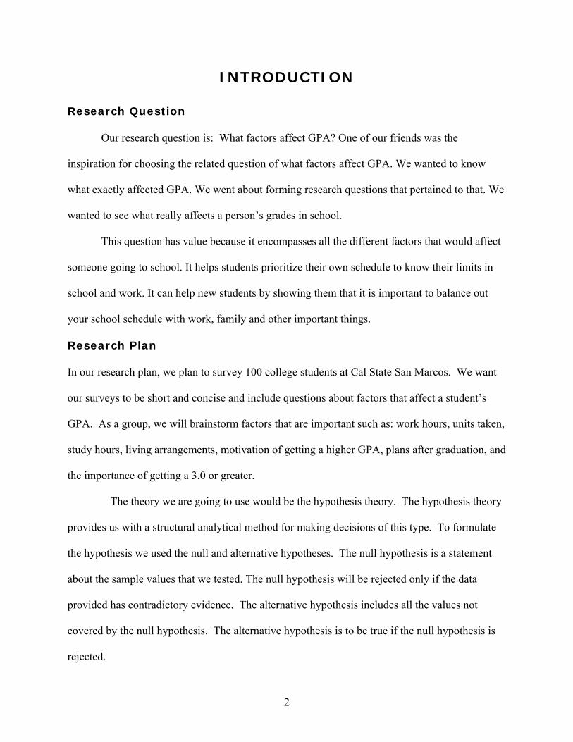
INTRODUCTION

Research Question

Our research question is: What factors affect GPA? One of our friends was the

inspiration for choosing the related question of what factors affect GPA. We wanted to know

what exactly affected GPA. We went about forming research questions that pertained to that. We

wanted to see what really affects a person’s grades in school.

This question has value because it encompasses all the different factors that would affect

someone going to school. It helps students prioritize their own schedule to know their limits in

school and work. It can help new students by showing them that it is important to balance out

your school schedule with work, family and other important things.

Research Plan

In our research plan, we plan to survey 100 college students at Cal State San Marcos. We want

our surveys to be short and concise and include questions about factors that affect a student’s

GPA. As a group, we will brainstorm factors that are important such as: work hours, units taken,

study hours, living arrangements, motivation of getting a higher GPA, plans after graduation, and

the importance of getting a 3.0 or greater.

The theory we are going to use would be the hypothesis theory. The hypothesis theory

provides us with a structural analytical method for making decisions of this type. To formulate

the hypothesis we used the null and alternative hypotheses. The null hypothesis is a statement

about the sample values that we tested. The null hypothesis will be rejected only if the data

provided has contradictory evidence. The alternative hypothesis includes all the values not

covered by the null hypothesis. The alternative hypothesis is to be true if the null hypothesis is

rejected.

3

Predictions

Before conducting the survey we believe that there will be strong and positive

correlations between working hours and the decrease in GPA, study hours and the increase in

GPA, unemployed students will have a higher GPA verses students who are employed. The

factor with the weakest correlation we predict will be commute time and it’s affect on GPA. The

more hours students spend working takes away from time that can be put towards their studies.

This is why we believe working hours and employed students will have a decrease affect on

GPA. Commute time affects each and every student, but the amount of effect we believe is

minimal.

METHODOLOGY

Research Procedure

Once we agreed on a research question, we decided that the best way to answer our

question was to conduct a survey. We felt that a survey would be the simplest and easiest

research method. Due to time constraints, we agreed to personally hand out surveys instead of

sending them to people through the Internet or mail. By handing out the surveys, we could get

responses immediately because we would not have to wait until respondents mailed the surveys

back to us or respond electronically. Also, we were guaranteed that for every survey we handed

out, we would get a completed survey back since surveys sent through mail or email have a

higher chance of getting ignored. It was also convenient to hand out the surveys personally

because we could just give them to classmates and acquaintances. Therefore, our sampling

technique was based on convenience sampling.

4

After we made the decision to conduct a survey, we began to brainstorm the factors that

would most likely affect GPA. With these factors in mind, each of us separately came up with

questions that relate to factors that affect GPA. We then combined our questions and removed

duplicate and irrelevant questions because we wanted to keep the ones that were significant.

After submitting the rough draft of our survey to the teacher, we further revised our questions so

that they would be more focused on the research question. During this process, we reworded the

questions so that respondents would know exactly how to respond. After revising the survey, we

were left with the 16 questions that we felt were the most relevant. It was really important that

our questionnaire be short (15-20 questions) and fit one page because we did not want to

overwhelm and discourage our respondents.

After we created our survey, we began discussion on how we were going to execute our

research. We decided to have a sample size of 100 respondents because we felt that it would be

feasible, considering our time constraints. To further expedite the surveying process, each

member of the group was to hand 25 surveys. This way, each person could hand the surveys out

to their respective classmates and acquaintances. After each person had their surveys filled out,

he/she inputted the results into Microsoft Excel. It was easier to input the results of 25 surveys

individually than inputting 100 surveys at once. We then combined our results to begin

analyzing.

Outcome

There were many advantages and disadvantages of our research methodology. It was

advantageous because it was efficient and quick. It was convenient because we handed out the

surveys to whomever we knew and was near. The convenience factor and the fact that it took

less than one minute to fill out the survey enabled us to get results immediately. However,

5

because the respondents were put on the spot, many answered our questions with estimations.

For instance, some did not know their GPA at the top of their head. Had they been on a

computer, they could have looked up more accurate information regarding their GPA on

SMART Web. Some answered the question hastily, possibly because of bad timing or because

they wanted to rush through the survey process. Finally, the fact that we kept the survey short

helped because everyone was willing to participate and, with exception of seven people,

completed the entire survey.

We could have reworded our questions to be clearer because some answered our

questions incorrectly. For instance, with our question, “What motivates you most in

getting/maintaining a high GPA (3.0 or greater)?” we wanted them to answer by choosing one of

the responses. However, some disregarded the word “most” and chose more than one answer.

This problem could have been avoided had we been clearer, by specifying that they choose one.

Also, since we passed out the surveys to classmates and acquaintances, the respondents

were characteristically too similar; our results were not as spread out. Therefore, our sample is

definitely not representative of the population in CSUSM.

The survey that was handed out to CSUSM students is shown on the next page.

6

Age __________ Gender __________ Marital status __________ Do you have children? YES NO What is your commute time to school? _____ minutes Do you participate in extracurricular (school-related) activities? YES NO If yes, how many hours do you spend on those activities a week? _____ Do you have a job? YES NO If yes, how many hours do you work a week? _____ What is your cumulative GPA? _____ How many units are you taking this semester? _____ How many hours do you spend studying a week?____ Who do you live with?

a) Parents b) Significant other and/or children c) Roommates d) Alone

What motivates you the most in getting/maintaining a high GPA (3.0 or greater)?

a) Acceptance to graduate school b) Attention of future employer(s) c) Outside motivation (i.e. pressure from parents, friends, etc.) d) Competition with fellow students e) Self-recognition f) Other ____________________________________________________

What are your plans after graduating from CSUSM?

a) Enroll in graduate school b) Start career c) Focus on family

How important is it for you to get/maintain a high GPA (3.0 or greater)?

Not Important Very Important 1 2 3 4 5

7

RESULTS

The following are the results of our survey. The questions of the survey can be broken up

into three categories: demographics, school, and outside school. We felt that all the questions

pertaining to these categories are relevant to our research. We included demographic questions

because we wanted to know who our respondents were and to determine their validity. The

school and outside school related questions were intended to help us find a commonality between

students who have GPA’s of 3.0 or higher versus those who have GPA’s lower than 3.0.

Demographics

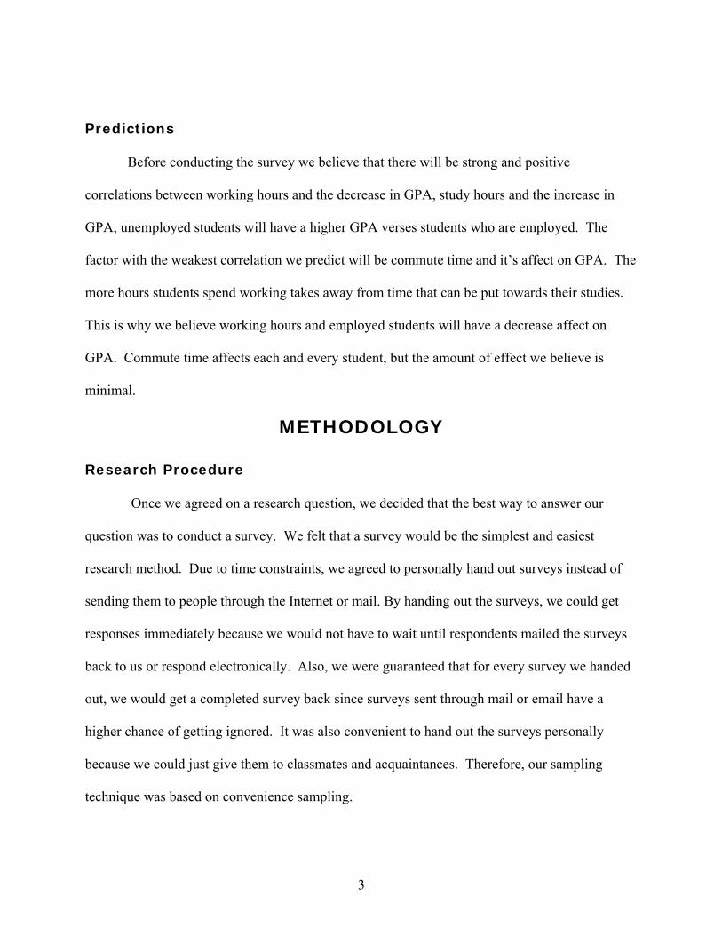
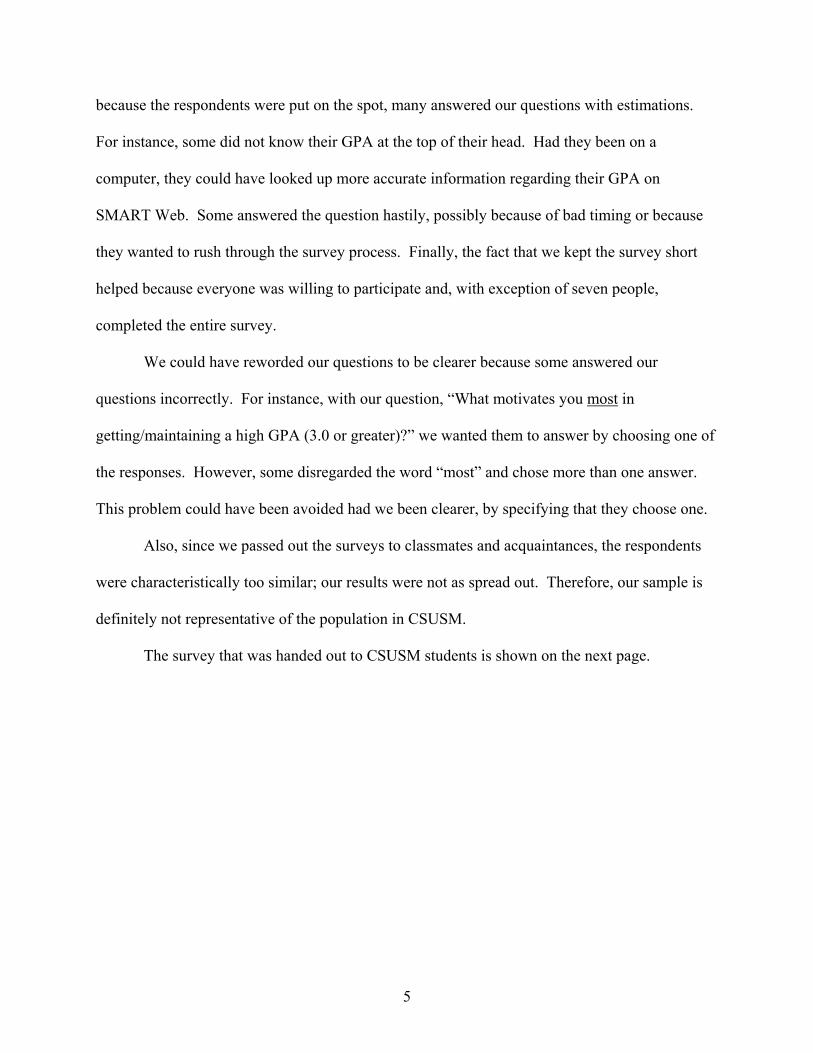
The mean, median, and mode age of our respondents is 23. Although the mean, median,

and mode of age are equal, the frequency distribution is right-skewed. Out of pure luck, the

amount of females and males that we surveyed were almost equal with 50 female respondents

and 43 male respondents. As expected—those surveyed were college students—the majority of

students was not married and did not have children. Only 13% were married and 11% had

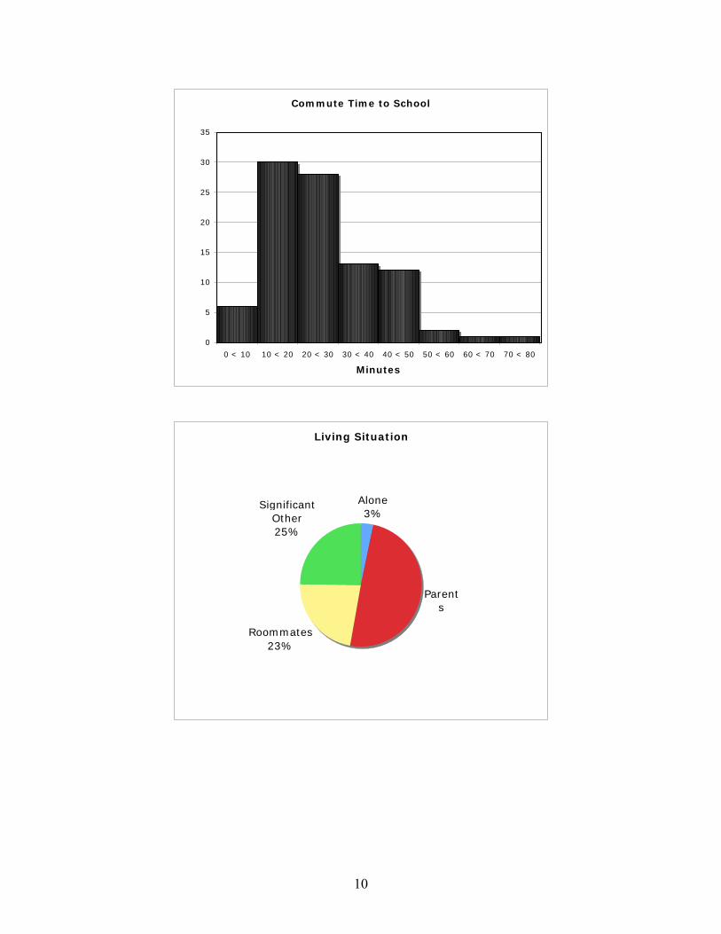
children. According to the right-skewed frequency distribution of commute time, most students’

drive to school takes 10 to 20 minutes. Lastly, almost half of the students we survey live with

their parents. We asked questions regarding marital status, children, commute time, and living

situation because we wanted to know if there was a correlation between these factors and GPA.

We believe that differing priorities, distractions, responsibilities, and time constraints would

affect GPA.

8

Respondent's Age

0

5

10

15

20

25

30

35

40

18 < 21 21 < 24 24 < 27 27 < 30 30 < 33 33 < 36 36 < 39 39 < 42

Age Range

Gender

38

40

42

44

46

48

50

52

Female Male

9

Marital Status

0

10

20

30

40

50

60

70

80

90

Married Single

Children

0

10

20

30

40

50

60

70

80

90

Yes No

10

Commute Time to School

0

5

10

15

20

25

30

35

0 < 10 10 < 20 20 < 30 30 < 40 40 < 50 50 < 60 60 < 70 70 < 80

Minutes

Living Situation

Alone3%

SignificantOther25%

Roommates23%

Parents

11

School

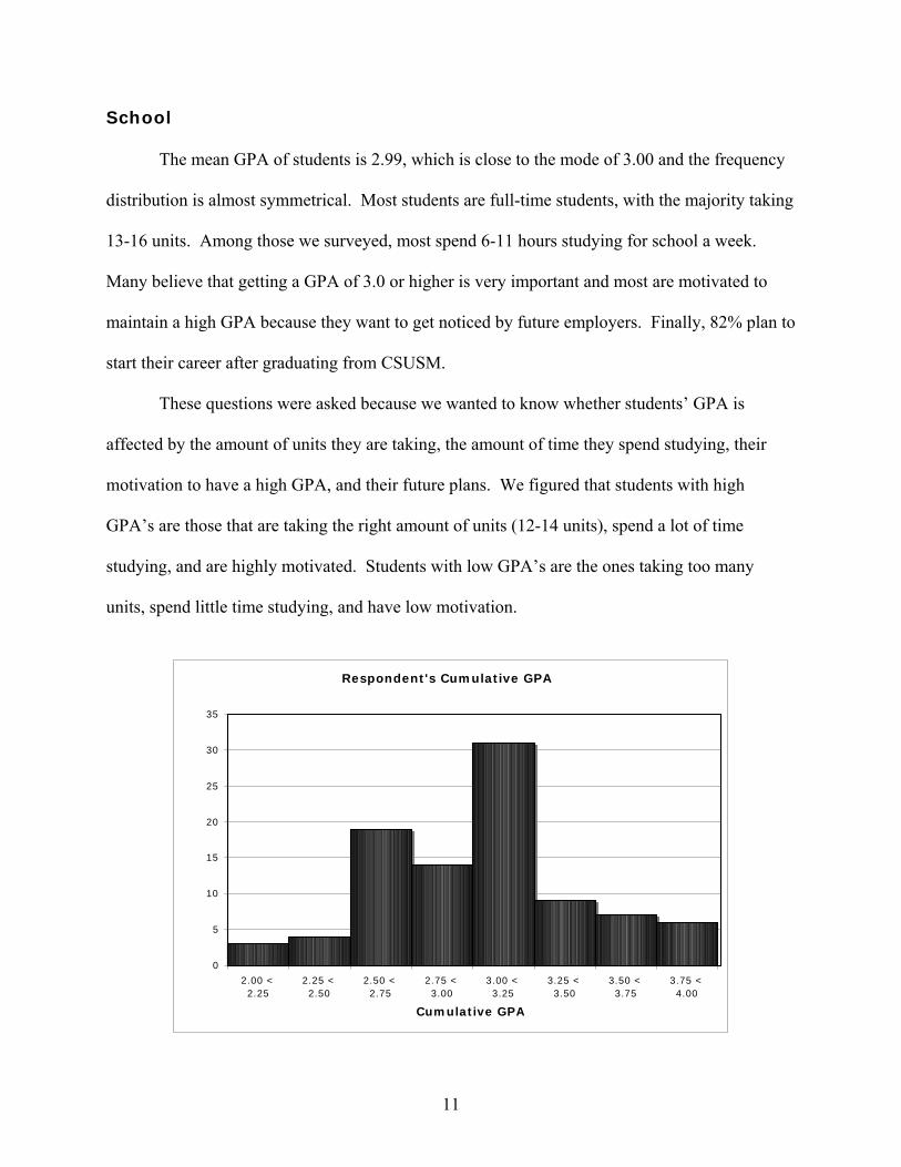
The mean GPA of students is 2.99, which is close to the mode of 3.00 and the frequency

distribution is almost symmetrical. Most students are full-time students, with the majority taking

13-16 units. Among those we surveyed, most spend 6-11 hours studying for school a week.

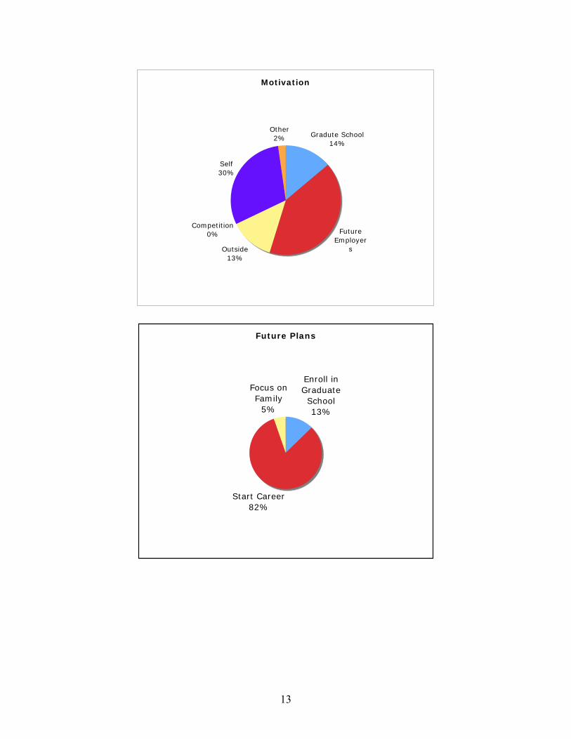
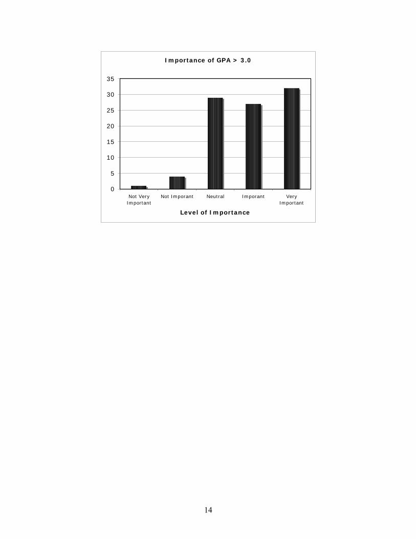
Many believe that getting a GPA of 3.0 or higher is very important and most are motivated to

maintain a high GPA because they want to get noticed by future employers. Finally, 82% plan to

start their career after graduating from CSUSM.

These questions were asked because we wanted to know whether students’ GPA is

affected by the amount of units they are taking, the amount of time they spend studying, their

motivation to have a high GPA, and their future plans. We figured that students with high

GPA’s are those that are taking the right amount of units (12-14 units), spend a lot of time

studying, and are highly motivated. Students with low GPA’s are the ones taking too many

units, spend little time studying, and have low motivation.

Respondent's Cumulative GPA

0

5

10

15

20

25

30

35

2.00 <2.25

2.25 <2.50

2.50 <2.75

2.75 <3.00

3.00 <3.25

3.25 <3.50

3.50 <3.75

3.75 <4.00

Cumulative GPA

12

Units Students are Taking

0

5

10

15

20

25

30

35

40

4 < 7 7 < 10 10 < 13 13 < 16 16 < 19

Units

Hours Spent Studying per Week

0

5

10

15

20

25

30

35

1 < 6 6 < 11 11 < 16 16 < 21 21 < 26 26 < 31 31 < 36 36 < 41

Hours

13

Motivation

Outside 13%

Competition0%

Self30%

Other2% Gradute School

14%

Future Employer

s

Future Plans

Enroll in Graduate School13%

Start Career82%

Focus onFamily

5%

14

Importance of GPA > 3.0

0

5

10

15

20

25

30

35

Not VeryImportant

Not Imporant Neutral Imporant VeryImportant

Level of Importance

15

Outside School

We believe that the busier students are, the greater the chance that their GPA’s were

going to be lower than those that mostly focuses on school. So we felt it was important to ask

questions regarding students’ lives outside of school.

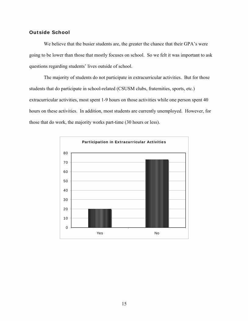
The majority of students do not participate in extracurricular activities. But for those

students that do participate in school-related (CSUSM clubs, fraternities, sports, etc.)

extracurricular activities, most spent 1-9 hours on those activities while one person spent 40

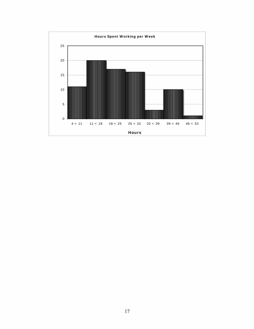
hours on these activities. In addition, most students are currently unemployed. However, for

those that do work, the majority works part-time (30 hours or less).

Participation in Extracurricular Activities

0

10

20

30

40

50

60

70

80

Yes No

16

Hours Spent on Extracurricular Activities per Week

0

2

4

6

8

10

12

14

16

1 < 9 9 < 17 17 < 25 25 < 33 33 < 41

Hours

Employment

0

10

20

30

40

50

60

70

80

90

Yes No

17

Hours Spent Working per Week

0

5

10

15

20

25

4 < 11 11 < 18 18 < 25 25 < 32 32 < 39 39 < 46 46 < 53

Hours

18

ANALYSIS

GPA AGE COMM TIME EA HRS WORK HRS UNITS STUDY

GPA 1 AGE 0.04967062 1 COMM TIME -0.0382282 -0.0378705 1 EA HRS -0.0523229 -0.123538 0.04036569 1 WORK HRS -0.1320484 0.12682592 -0.0267086 -0.0258425 1

UNITS 0.18181975 -0.2420766 0.05111876 0.18664791 -

0.2636274 1

STUDY 0.02034314 0.26456598 0.01320398 0.07834934 -

0.1096085 0.37468962 1

SUMMARY OUTPUT

Regression Statistics

Multiple R 0.2621

R Square 0.0687

Adjusted R Square 0.0037

Standard Error 0.4177

Observations 93

ANOVA

df SS MS F Significance

F

Regression 6 1.1071 0.1845 1.0577 0.3944

Residual 86 15.0038 0.1745

Total 92 16.1110

Coefficients Standard Error t Stat P-value Lower 95% Upper 95% Lower 95.0% Upper 95.0%

Intercept 2.3277 0.4280 5.4385 0.0000 1.4769 3.1786 1.4769 3.1786

Age 0.0160 0.0132 1.2109 0.2293 -0.0102 0.0422 -0.0102 0.0422

Commute Time -0.0013 0.0031 -

0.4197 0.6758 -0.0075 0.0049 -0.0075 0.0049 Extracurricular Activities -0.0066 0.0096

-0.6853 0.4950 -0.0257 0.0125 -0.0257 0.0125

Work Hours -0.0033 0.0035 -

0.9251 0.3575 -0.0103 0.0038 -0.0103 0.0038

Semester Units 0.0370 0.0186 1.9930 0.0494 0.0001 0.0739 0.0001 0.0739

Study Time -0.0063 0.0066 -

0.9421 0.3488 -0.0195 0.0069 -0.0195 0.0069

19

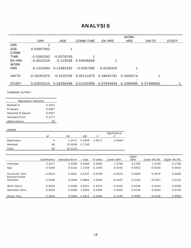
According to the multiple regression analysis we ran through Microsoft Excel, our model

is not significant because the Significance F of 0.3944. Even though we knew that our model is

not significant we decided to examine each of the factors separately to see if they correlate.

We first analyzed whether there was a correlation between the number of units a person

is taking and the student’s cumulative GPA. Our hypothesis was that the more units students are

taking, the lower their GPA is going to be. We made this conclusion because overloading on

units can lead students to work less effectively because they have to worry about more classes.

Although the relationship is not significant, there apparently is a negative correlation between the

two factors. Therefore, our claim is somewhat.

20

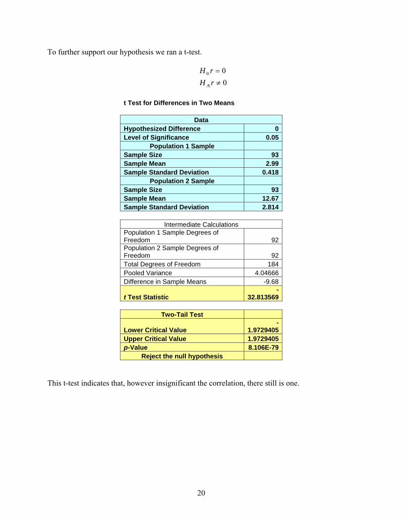
To further support our hypothesis we ran a t-test.

00

:

:0

≠=

rHrH

A

t Test for Differences in Two Means

Data Hypothesized Difference 0Level of Significance 0.05

Population 1 Sample Sample Size 93Sample Mean 2.99Sample Standard Deviation 0.418

Population 2 Sample Sample Size 93Sample Mean 12.67Sample Standard Deviation 2.814

Intermediate Calculations Population 1 Sample Degrees of Freedom 92Population 2 Sample Degrees of Freedom 92Total Degrees of Freedom 184Pooled Variance 4.04666Difference in Sample Means -9.68

t Test Statistic -

32.813569

Two-Tail Test

Lower Critical Value -

1.9729405Upper Critical Value 1.9729405p-Value 8.106E-79

Reject the null hypothesis

This t-test indicates that, however insignificant the correlation, there still is one.

21

We then did a two tail test on one sample with the following results. This t test was for

hours worked. We hypothesized that the more hours worked means the less time for students to

study and it shows in the correlation. It shows that we should reject the null hypothesis, the

upper and lower critical values. There was no correlation, and therefore we should reject the null

hypothesis.

22

t Test for Differences in Two Means

Data Hypothesized Difference 0Level of Significance 0.05

Population 1 Sample Sample Size 93Sample Mean 18.92Sample Standard Deviation 12.79

Population 2 Sample Sample Size 93Sample Mean 2.99Sample Standard Deviation 0.418

Intermediate Calculations Population 1 Sample Degrees of Freedom 92Population 2 Sample Degrees of Freedom 92Total Degrees of Freedom 184Pooled Variance 81.879412Difference in Sample Means 15.93t Test Statistic 12.004799

Two-Tail Test

Lower Critical Value -

1.9729405Upper Critical Value 1.9729405p-Value 6.815E-25

Reject the null hypothesis

23

The null and alternative hypotheses are:

0:0:0

≠=

rHrH

A

Correlation = -0.0382282

24

t Test for Hypothesis of the Mean

t Test for Hypothesis of the

Mean

Data Data

Null Hypothesis

µ= 0 Null Hypothesis µ= 0

Level of Significance 0.05 Level of Significance 0.05

Sample Size 94 Sample Size 94

Sample Mean 23.215054 Sample Mean 2.99

Sample Standard

Deviation 14.0103538 Sample Standard Deviation 0.418

Intermediate Calculations Intermediate Calculations

Standard Error of the Mean 1.445057658 Standard Error of the Mean 0.043113408

Degrees of Freedom 93 Degrees of Freedom 93

t Test Statistic 16.06514029 t Test Statistic 69.35197499

Two-Tail Test Two-Tail Test

Lower Critical Value

-

1.985801768 Lower Critical Value

-

1.985801768

Upper Critical Value 1.985801768 Upper Critical Value 1.985801768

p-Value 1.42657E-28 p-Value 7.0767E-82

Reject the null hypothesis Reject the null hypothesis

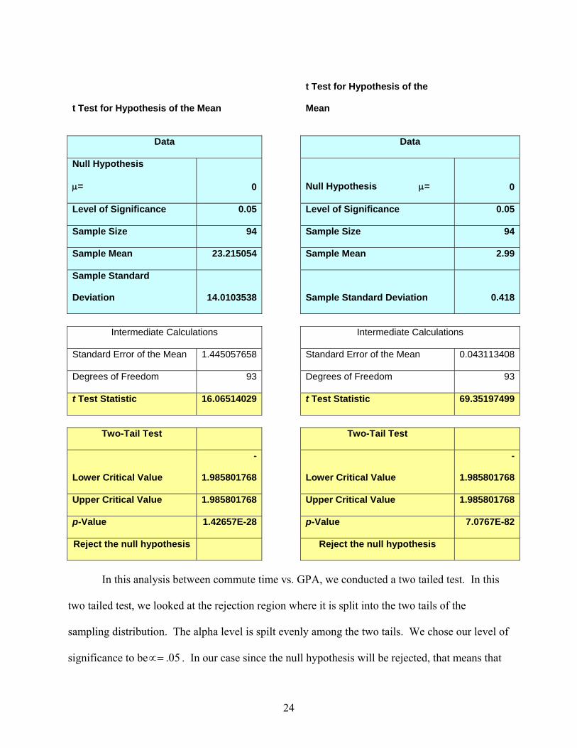
In this analysis between commute time vs. GPA, we conducted a two tailed test. In this

two tailed test, we looked at the rejection region where it is split into the two tails of the

sampling distribution. The alpha level is spilt evenly among the two tails. We chose our level of

significance to be 05.∝= . In our case since the null hypothesis will be rejected, that means that

25

the sample mean is extremely larger or extremely smaller. From our data, the p-value of in GPA

is significantly smaller than commute time. This tells us that the smaller the p-value than the

probability is in the rejection region, then the null hypothesis is rejected. In both of these cases,

however are both rejected because they fall outside of the region of given hypothesis.

We believe there will be a strong correlation between the hours that a student spends

studying and their GPA. Below is the graph of sample data we collected.

To test out our sample of interest we formed the hypothesis :

oH : 0<r

AH : 0>r

α=0.05

With a sample size of 93 our degree of freedom is 91. Below is a t-test that was performed for

these to sample means. By looking at the result of the PHStat we can see that the critical value

1.65; therefore our decision rule was:

If t > 1.65 reject the null hypothesis, otherwise do not reject.

26

 t Test for Differences in Two Means

Data Hypothesized Difference 0Level of Significance 0.05

Population 1 Sample Sample Size 93Sample Mean 12.65Sample Standard Deviation 7.71

Population 2 Sample Sample Size 93Sample Mean 2.99Sample Standard Deviation 0.418

Intermediate Calculations Population 1 Sample Degrees of Freedom 92Population 2 Sample Degrees of Freedom 92Total Degrees of Freedom 184Pooled Variance 29.809412Difference in Sample Means 9.66t Test Statistic 12.064988

Upper-Tail Test Upper Critical Value 1.6531771p-Value 2.266E-25

Reject the null hypothesis  t= 12.065, thus 12.065 > 1.65, therefore we reject the null hypothesis. Because the null

hypothesis was rejected the sample showed there was a correlation between study hours and

GPA.

The following are the results to our qualitative data. Because we were working with non-

quantitative data, we decided to analyze these factors differently. We decided to find the mean

GPA of each category to determine any trends.

27

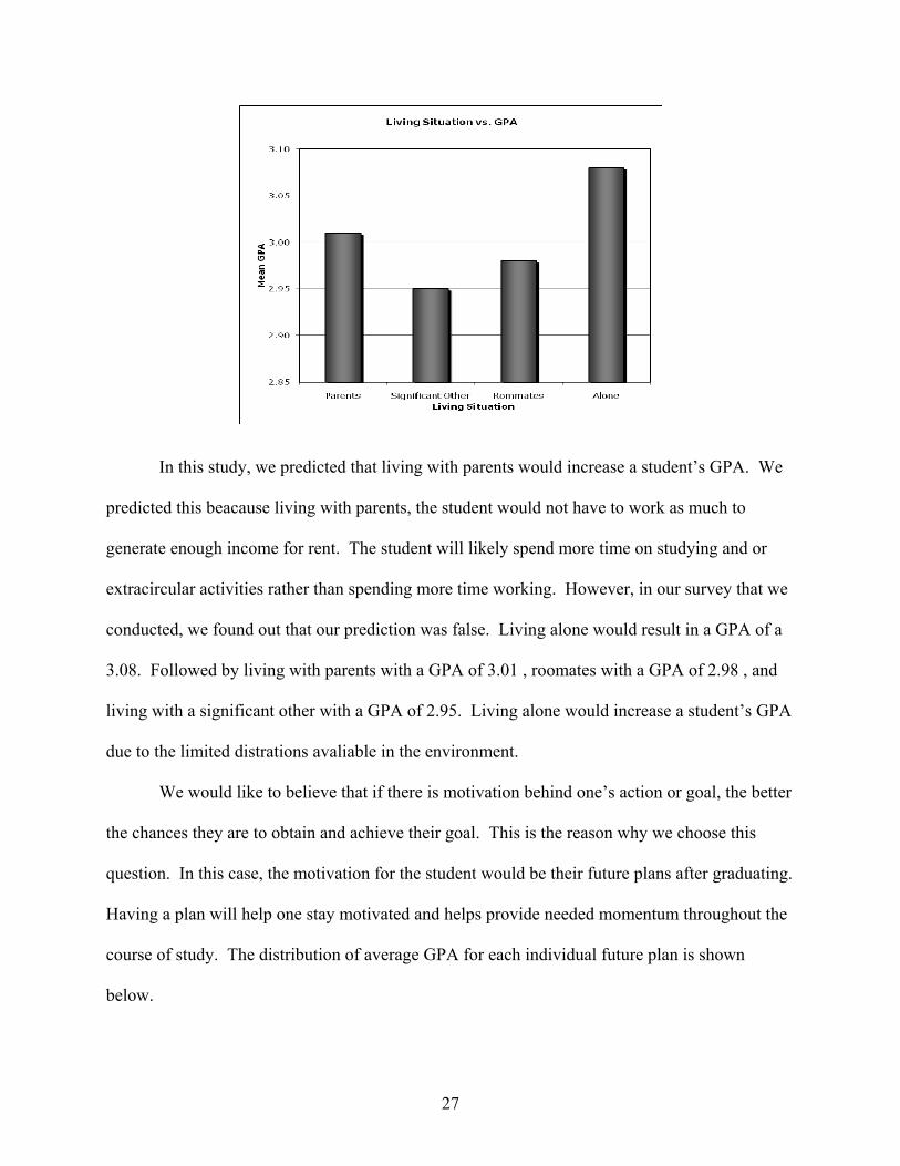
In this study, we predicted that living with parents would increase a student’s GPA. We

predicted this beacause living with parents, the student would not have to work as much to

generate enough income for rent. The student will likely spend more time on studying and or

extracircular activities rather than spending more time working. However, in our survey that we

conducted, we found out that our prediction was false. Living alone would result in a GPA of a

3.08. Followed by living with parents with a GPA of 3.01 , roomates with a GPA of 2.98 , and

living with a significant other with a GPA of 2.95. Living alone would increase a student’s GPA

due to the limited distrations avaliable in the environment.

We would like to believe that if there is motivation behind one’s action or goal, the better

the chances they are to obtain and achieve their goal. This is the reason why we choose this

question. In this case, the motivation for the student would be their future plans after graduating.

Having a plan will help one stay motivated and helps provide needed momentum throughout the

course of study. The distribution of average GPA for each individual future plan is shown

below.

28

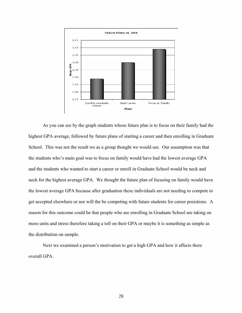
As you can see by the graph students whose future plan is to focus on their family had the

highest GPA average, followed by future plans of starting a career and then enrolling in Graduate

School. This was not the result we as a group thought we would see. Our assumption was that

the students who’s main goal was to focus on family would have had the lowest average GPA

and the students who wanted to start a career or enroll in Graduate School would be neck and

neck for the highest average GPA. We thought the future plan of focusing on family would have

the lowest average GPA because after graduation these individuals are not needing to compete to

get accepted elsewhere or nor will the be competing with future students for career posistions. A

reason for this outcome could be that people who are enrolling in Graduate School are taking on

more units and stress therefore taking a toll on their GPA or maybe it is something as simple as

the distribution on sample.

Next we examined a person’s motivation to get a high GPA and how it affects there

overall GPA.

29

Our hypothesis was that the more motivation a student had he/she would have a higher

GPA then students that did not have any or little motivation. Above is the bar graph showing the

outcomes from graphing motivation vs. GPA. With motivation consisting of 5 different options,

most students with any form of motivation had a higher GPA then other students with less

motivation. Therefore we can conclude from the above results that any form of outside

motivation can help increase Student’s overall grades.

We then looked at how the level of importance affects GPA.

30

We wanted to determine whether a person's GPA is dependent on how important

getting/maintaining high GPA is to them. Our conclusion is that people who view having a high

GPA will most likely have higher GPA's because they are more likely put more effort into

studying hard to get better grades. On the other hand, people that do not consider a high GPA to

be important will most likely take the attitude of just wanting to get by and pass their classes.

When students have this attitude, they will mostly likely have lower GPA’s. Surprisingly, the

highest mean GPA belonged to the group of people that do not consider a high GPA of being

important. However, as the level of importance increased, the more the mean GPA increased.

This further supports our theory that the more important it is for someone to have a high GPA,

the more likely their GPA will be high.

CONCLUSION

In this research, we surveyed 100 college students at Cal State San Marcos. We

surrounded our questions on motivational factors on getting a high GPA. We considered

important factors such as the amount of works hours in a given week, units taken during the

semester, study hours on an average week, living arrangements, motivation of getting a higher

GPA, and the importance of achieving a 3.0 or greater to the student. From our data, we

determined that the most of our factors had no significant correlation except for study hours vs.

GPA. This comparison looked to have a stronger correlation because the more hours spent

studying the higher the student’s GPA will be. The weakest correlation that we determined

would be commute time because it did not have any significance due to the miles driven verses

the student’s GPA. From our study, we can conclude that many factors can affect a student’s

GPA. The amount of study hours is most significant because the amount of hours a student

31

studies, determines the grade received in each class and then the outcome at the end of semester

is to receive a high GPA.