Factorgrams: A tool for visualizing multi-way associations in

http://www.psi.toronto.edu

Factorgrams: A tool for visualizing multi-wayassociations in biological data

Vincent Cheung, Inmar Givoni, Delbert Dueck, Brendan J. Frey

May 15, 2006 PSI TR 2006–44

Abstract

Effective visualization of biological data is often critical for subsequent analy-sis. The popular clustergram/dendrogram visualization rearranges rows andcolumns of a data matrix so as to highlight clusters of similar responses, butassumes each row or column belongs to only one cluster and cannot associateeach row or column with multiple clusters. Such multi-way associations oc-cur frequently, e.g., when a gene plays multiple biological roles. We describethe ’factorgram’ visualization, which rearranges the data into an expandedview, associating each row (or column) with multiple clusters of rows (orcolumns) and elucidating potentially new biological relationships. Factor-grams for mouse gene expression and yeast synthetic-lethal gene-interactiondatasets detect a larger number of statistically-significant clusters than clus-tergrams, plus a larger number of clusters enriched for gene ontology annota-tions. Experimentally-verified associations previously identified by manualrearrangement of rows and columns not grouped together by clustergrams,are readily identified by the factorgram.

Factorgrams: A tool for visualizing multi-way associations in biological data

Vincent Cheung1,2, Inmar Givoni1,2, Delbert Dueck1,2, Brendan J. Frey2,3,4

1. These authors contributed equally 2. Probabilistic and Statistical Inference Group, Departments of Electrical and

Computer Engineering and Computer Science, University of Toronto, 10 King’s College Rd., Toronto, ON, Canada, M5S 3G4

3. Banting and Best Department of Medical Research, University of Toronto, 112 College St., Toronto, ON, Canada, M5G 1L6

4. To whom correspondence should be addressed: Brendan J. Frey, [email protected], 416-978-7001 (office), 416-978-4425 (fax).

Effective visualization of biological data is often critical for subsequent analysis.

The popular clustergram/dendrogram visualization rearranges rows and columns of a

data matrix so as to highlight clusters of similar responses [1], but assumes each row

or column belongs to only one cluster and cannot associate each row or column with

multiple clusters. Such multi-way associations occur frequently, e.g., when a gene

plays multiple biological roles. We describe the ‘factorgram’ visualization, which

rearranges the data into an expanded view, associating each row (or column) with

multiple clusters of rows (or columns) and elucidating potentially new biological

relationships. Factorgrams for mouse gene expression and yeast synthetic-lethal gene-

interaction datasets detect a larger number of statistically-significant clusters than

clustergrams, plus a larger number of clusters enriched for gene ontology

annotations. Experimentally-verified associations previously identified by manual

rearrangement of rows and columns not grouped together by clustergrams, are

readily identified by the factorgram.

Factorgrams – Cheung et al.

2

High-throughput biological assays produce huge quantities of data, which can often be

organized into a matrix where rows and columns correspond to separate control variables,

and each element in the matrix is a binary- or real-valued measured response. For example,

the rows may correspond to microarray probes for genes, exons or tiled DNA segments, the

columns to time points or tissue samples, and each element to a real-valued transcript

abundance estimated using a microarray. Or, the rows and columns may correspond to

yeast genes and each element to a binary value indicating whether or not there is a

synthetic lethal interaction in the yeast strain with both genes deleted. While customized

techniques based on machine learning and statistical inference can be used to analyze this

kind of data, even simple rearrangements of the data or straightforward transformations of

the data can reveal biologically-significant patterns that are directly visualized in the

rearranged dataset. Currently, the most common visualization tool for biological matrix

data is the clustergram, in which the rows and the columns of the data matrix are re-ordered

using a clustering method such as hierarchical agglomerative clustering (HAC) [11] or k-

means clustering [12]. Similarities between nearby rows or columns may be indicated by

dendrogram. The rearranged matrix of data is shown as an image where the color at each

coordinate corresponds to the appropriate binary- or real-valued response [1].

A major deficiency of clustergrams is that rows (or columns) are grouped together

based on similarity of response across their entire columns (or rows). In many biological

assays, it is frequently the case that different biological processes will impact overlapping,

but not disjoint, sets of variables. For example, consider a yeast synthetic gene interaction

matrix in which rows correspond to gene deletion mutants of different non-essential yeast

genes, columns also correspond to gene deletion mutants of non-essential yeast genes, and

each element in the matrix measures the viability of a yeast strain with both genes knocked

out. If genes A and B exhibit similar viability patterns across a subset of other genes, they

can be grouped together, indicating that they may be part of the same functional pathway

involving all genes in the subset. However, gene B may additionally play a different

biological role as part of another pathway that does not involve gene A, but involves gene

C. Genes B and C may exhibit similar viability patterns across a different subset of genes,

namely those that are involved in the second pathway. In this case, there are two clusters


3

corresponding to the two pathways and they overlap in the sense that they both contain

gene B. This creates a problem for clustering methods, which assume that clusters do not

overlap. Standard clustering techniques and the clustergram visualization do not provide a

general way to link gene B to both genes A and C, what we refer to as making ‘multi-way

associations’.

The failure of the clustergram to indicate multi-way associations is evident from the

data of Tong et al. [13], shown in Fig. 1A by ordering the rows and columns according to

the dendrograms produced by HAC (see Methods). Each row or column can only be

associated with nearby rows or columns, so overlapping clusters of genes (i.e., multi-way

associations) are not properly revealed. In Fig. 1B we highlight two examples of data

clusters that are significantly enriched for gene function annotations, but that were not

properly identified by hierarchical clustering and were thus broken apart in the clustergram.

In some cases, a row or column can be visually associated with two clusters if by

coincidence it is on the boundary between the two clusters or if a computational method is

used to move it to a position that is closer to another cluster. However, clustergrams cannot

generally reveal all such double-associations, because only a small number of cases can be

placed near cluster boundaries.

The ‘factorgram’ is a visualization that expands the input data matrix so as to enable

explicit visualization of data in overlapping clusters. We refer to each such overlapping

cluster as a ‘factor’, because techniques that explain each row or column of data as a

composition of multiple components are called ‘factorization’ methods in the machine

learning and statistics communities, and each component is called a ‘factor’ (c.f. [2]). The

output from a variety of factorization techniques [2-10] can be further processed to produce

the factorgram. The purpose of this paper is not to advocate a particular factorization

technique, but to illustrate how the factorgram visualization can be useful to biologists for

further analysis and detection of a larger number of statistically and biologically significant

associations than cannot be detected using clustergrams. Software for producing

factorgrams is available at http://www.psi.toronto.edu/factorgram.


4

To give the reader a sense for how factorgrams work, in Fig. 2 we show a cartoon

illustrating one way to construct a factorgram. The clustergram of a synthetic binary data

matrix is shown in the upper-left corner, and includes blocks of data that have been broken

apart because specific rows and columns (shown with arrows) belong to multiple groups.

To produce the factorgram, the rows and columns are rearranged so that the dominant

factor appears as a contiguous block of data. This factor is then removed from the matrix

and placed in the factorgram. The rows and columns of the resulting matrix are again

rearranged so that the next dominant factor appears as a contiguous block of data. This

factor is removed and placed in the factorgram. This procedure is repeated until no more

significant factors remain in the data matrix. The factorgram is a figure showing the raw

data associated with all extracted factors and may additionally include appropriate row and

column labels. The factors may be shown along the diagonal of a matrix to reflect

similarities to the clustergram, or the factors can be arranged more compactly. Since the

same row (or column) can appear in multiple factors, the factorgram provides a way to

visualize clusters with overlapping variables.

Techniques for computing factorgrams should properly address how to efficiently

search over possible solutions and assess the statistical significance of the detected factors.

In contrast to clustergrams, where each row or column is associated with one cluster, in

factorgrams, each row or column can be associated with multiple factors through different

subsets of responses. This capability comes at the cost of an exponentially larger space of

possible solutions, since if there are k factors and each row or column can belong to n

factors at once, there are kn possible ways of assigning the row or column to the factors.

Approaches for efficiently searching over these assignments include computing linear

approximations and using more powerful probabilistic inference techniques. A binary

assignment variable with value 0 or 1 can be used to indicate whether or not a row or

column belongs to a factor. If these assignment variables are relaxed to be real-valued, data

elements are described by linear combinations of continuous variables. Continuous

solutions to the factorization problem can be computed using an eigen-vector method such

as principal components analysis [3] or an iterative technique such as factor analysis [2],

independent component analysis [4] and non-negative matrix factorization [5]. Once the


5

real-valued ‘assignment’ variables have been computed, they can be thresholded to identify

components in the factorgram. One problem with these approaches is that a good binary

solution often cannot be obtained by thresholding the best continuous solution. An

alternative approach is to retain the binary representation of the assignment variables but

constrain the solution space. Bi-clustering [6] imposes the constraint that any two clusters

containing the same column (or row) must be defined by exactly the same set of columns

(or rows); this constraint makes extraction of factors easier, but is only appropriate when

different factors are defined by the same subsets of rows or columns.

Recently, methods have been proposed that retain the binary representation of the

assignment variables and avoid simplifying assumptions about the factors by using

techniques developed in the probabilistic and statistical inference communities to search for

the most probable setting of the assignment variables. The plaid method [7] works by

extracting one factor at a time using the linear approximation described above, but then

thresholds the assignment variables before proceeding to extract the next factor.

Probabilistic sparse matrix factorization [8,9] and matrix tile analysis [10] take a direct

approach and retain the binary representation, but find solutions by accounting for

uncertainties in the assignments and iteratively revisiting and refining factors until

convergence. The labelled latent Dirichlet allocation process analysis method [15] takes as

input the data matrix along with gene function annotations and performs Bayesian

inference in a hierarchical probabilistic graphical model to extract the factors.

The statistical significance of the factors in a factorgram can be assessed in a variety of

ways, but here we describe a general procedure that can be applied to any technique that

computes a factorgram. Denote the data matrix by X and the particular method used to

compute the factorgram by μ. We assume the method takes as input the data matrix and a

parameter θ that indirectly has an impact on the false detection rate. For example, θ could

be a real-valued threshold on a cost function that penalizes small factors (which are less

likely to be significant) but rewards factors containing highly similar data elements. For

method μ applied to data X using parameter θ, denote the number of extracted factors by

N(X,μ,θ). The null hypothesis is that a computed factor arose from random data with the


6

same distribution as the source that produced X. Assuming the data matrix is large enough,

this distribution can be approximated by generating permuted data matrices (i.e., randomly

rearranging elements). Denote a data matrix obtained in this way by XR – since the data

elements were randomly rearranged, XR is a random variable. The expected number of

falsely detected factors can be estimated by E[N(XR,μ,θ)], where E[ ] denotes an

expectation w.r.t. the set of random matrices, XR. In this procedure, N(XR,μ,θ) is random

because XR is random, but also possibly because the method μ may produce different

solutions each time it is applied due to varying initial conditions.

We demonstrate the factorgram visualization using two publicly available datasets, the

yeast synthetic genetic array (SGA) dataset from Tong et al. [13] and the mouse gene

expression dataset from Zhang et al. [16]. The former is binary valued while the latter is

real-valued, and each dataset was factorized using a different method. However, the final

results are both readily visualized by the factorgram.

The SGA data is a binary-valued matrix of 135 by 1023 elements, where both rows

(query genes) and columns (array genes) correspond to yeast genes. Each element

represents the synthetic lethality of a double mutant whose corresponding row and column

genes have been knocked out. We applied HAC to both the rows and the columns of the

data matrix (see Methods) and in Fig. 1A we show the clustergram. The factorgram

generated from this data matrix (see Methods) contained 17 factors, 5.4 of which are

expected to be false detections based on the method described above, using ten random

permutation tests. The factorgram for the SGA data is shown in Fig. 3A, where each box

corresponds to one of the factors. While in the data matrix, only 3.35% of the gene pairs

exhibit synthetic lethality, in the identified set of factors 88.87% of the gene pairs exhibit

synthetic lethality. The identified factors account for 49.57% of the total number of

synthetic lethal interactions; 22.75% of the observed synthetic lethal interactions

correspond to array genes have three or less synthetic lethal interactions with query genes

and thus provide only weak evidence. In Fig. 3B, we show the clustergram obtained using

HAC (see Methods). We tried several clustering techniques and chose the one that

produced the largest number of biologically significant clusters (see below). In this figure,


7

each element assigned to a factor is coloured so as to indicate the factor in Fig. 3A to which

it belongs. The clustergram breaks apart almost every identified factor, thus failing to

associate all genes within each factor.

An example of a well known biological pathway that is not readily identified in the

clustergram in Fig. 3A is the chitin synthase III pathway (SKT5, CHS3, CHS5, CHS7),

which is grouped together in the factorgram (dark green factor in Fig. 3). In some cases, the

clustergram correctly groups query genes, but fails to group array genes. For example,

query genes in the prefoldin complex (GIM3, GIM4, GIM5, PAC10, YKE2) were correctly

grouped in the clustergram, but corresponding array genes were not properly identified (red

factor in Fig. 3). The clustergram produced by Tong et al. used a different metric and

successfully grouped genes in the synthase III pathway, but failed to group together array

associated with the prefoldin complex. Instead, this complex was identified by laborious

manual rearrangement of the partial clusters. The large red factor shown in Fig. 3

successfully brings together similarities of array gene profiles and query gene profiles, thus

capturing both the row-based similarities and the column based similarities of the gene

profiles. Furthermore, the dark purple factor shows how the query genes of the prefoldin

complex are also similar based on their symmetric interaction as array genes, a relationship

that again was neither captured in our clustergram nor reported by Tong et al.

We next asked how many of the extracted factors are of biological significance in terms

of functional enrichment. We analysed whether the genes in each cluster were significantly

enriched for gene ontology (GO) annotations of biological process, molecular function, and

cellular component. We found 9 of the clusters to be enriched (p < 0.01) for at least one

annotation, with a total of 18 significant enrichments across all three categories (see

Methods). In comparison, when we used HAC to find the same number of clusters, we

were able to find only 4 clusters to be enriched for at least one annotation, with a total of

only 7 significant enrichments across all three categories. We tried a variety of different

clustering techniques, but these resulted in lower numbers of enriched clusters (data not

shown).


8

The second dataset we analyzed and applied the factorgram visualization to is the

mouse mRNA expression dataset from Zhang et al. [16]. This dataset contains profiles for

over 22,709 known and predicted genes across 55 mouse tissues, organs, and cell types.

The factorgram generated from this dataset (see Methods) contained 37 factors and based

on the random permutation test we found that 0.5 factors are expected to be false

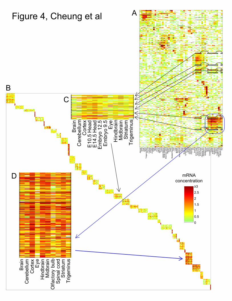
detections. The clustergram and factorgram are shown in Fig. 4. The factorgram correctly

identified many associations that are identified in the clustergram. For example, the cluster

containing nervous system tissues (inside the dark green bounding box in Fig. 4A) is

contained within the factor shown in Fig. 4D. Fig. 4C shows an example where the

discovered factor has been severely broken apart in the clustergram. This factor includes

genes that are expressed in both mature and embryonic nervous system tissues, and

includes genes not present in the previously described factor. Both of these factors have

statistically significant (p < 0.05) enrichment in gene annotations (see Methods).

Many factors reveal profile similarities across tissues which are not obviously similar,

and may seem surprising at first. However, this is one of the advantages of factorization

methods and of the factorgram, as they have the potential to enable the researcher to

scrutinize more interesting relationships. To answer the question of whether the additional

relationships detected in the factorgram are of biological significance, we analyzed the

factors for enrichment in GO biological process (GO-BP) annotations (see Methods). We

studied how many biologically significant groups were revealed in the factorgram

compared to other techniques for a fixed number of detected groups. In this case, parameter

θ controls the number of factors discovered in the data. We varied θ from 20 to 60 and

compared the genes in each factor with GO-BP annotations. Table 1 reports the number of

statistically significant factors (p < 0.05) for each θ-value; we also report corresponding

results for HAC. In general, the factogram reveals a larger number of significantly enriched

clusters.


9

Table 1: Comparison of number of clusters or factors enriched for GO-

BP annotations for different numbers of extracted clusters/factors.

Number of clusters/factors, θ

Number of enriched factors in factorgram

Number of enriched clusters in clustergram

20 16 13 30 21 15 40 26 17 50 28 19 60 32 20

Just as Eisen et al. [1] demonstrated that the clustergram provides a visual tool enabling

biologists to gain leads to interesting associations, our goal in writing this paper was to

demonstrate the advantages of the factorgram visualization in revealing multi-way

associations and enabling biologists to detect multiple associations. Unlike clustergrams,

where the number of salient associations is limited by the two-dimensional arrangement of

the data, factorgrams extract many two-dimensional arrangements so as to identify multiple

associations. We are not advocating a specific computational technique for factorizing the

data matrix, but are instead introducing and advocating the factorgram as a way to visualize

the outputs from a variety of computational techniques [2-10], each of which is appropriate

in specific situations. Factorgrams can be used to visualize the output of these techniques,

regardless of whether each element in the generated factors belongs to only one factor or to

multiple factors. In our experiments on synthetic lethal yeast gene interaction data and

mouse gene expression data, we found that factorgrams reveal a larger number of

statistically significant and biologically significant clusters compared to the number

revealed in clustergrams by HAC.

As a general tool for analyzing matrices of data, the factorgram can potentially have

broad application in detecting associations in biological data. The factorgram has been

recently applied to chemical-genetic interaction data in yeast to identify associations

between chemical compounds and genes [17]. It has also been used to identify relationships

between hundreds of genes involved in transcription [18]. New large-scale microarray

datasets for the study of mammalian alternative splicing have also recently been analyzed


10

using factorgrams [19]. Software for automatically producing factorgrams is available at

http://www.psi.toronto.edu/factorgram. Due to its simplicity, ease of computation, and

potential for revealing novel biological insights, we believe the factorgram will prove to be

a useful tool for visualizing multi-way associations in high-throughput biological data.

Methods

1. Yeast gene deletion data analysis.

The clustergram was produced using the MATLAB implementation of hierarchical

agglomerative clustering (HAC). We used Hamming distance, Euclidean distance,

correlation and city-block pseudo-distance functions with average and single linkage and

report results for Hamming distance with average linkage, which obtained the largest

number of clusters enriched for GO annotations.

The factorgram was produced using ‘matrix tile analysis’ based on an iterated

conditional modes technique [10]. Matrix tile analysis takes as input a matrix, where each

element is the log-ratio of probabilities that the element belongs in a factor and does not

belong in a factor. If a synthetic lethal interaction was observed between two pairs of genes

in the dataset of Tong et al. [13], we set the log-ratio to be log((1-ε)/ε) and otherwise we set

it to be log(ε/(1-ε)), where ε is the noise probability set to 0.0335, based on the average

number of observed synthetic lethal interactions. The parameter θ, which indirectly

determines the false detection rate by weighting the benefit of explaining the data to the

cost of introducing additional factors, was set to 0.15.

2. Mouse gene expression data analysis.

The clustergram was produced using the MATLAB implementation of HAC with

Pearson correlation and average linkage, which was selected for visualizing results by

Zhang et al. [16].

For the factorgram, we tried a different factorization technique from above called

‘probabilistic sparse matrix factorization’ (PSMF) [8,9]. Each expression measurement of a


11

gene in each tissue in the input matrix is represented by the arcsinh (approximately the

logarithm) of the ratio of normalized intensity of the gene in the given tissue to the gene’s

median normalized intensity across all 55 tissues. Observing that the majority of genes

expressed in any tissue were expressed in less than half of the tissues, Zhang et al. set ratios

less than one equal to one, reasoning that these ratios represent noise rather than down-

regulation thus the data is entirely non-negative.

PSMF discovers a large predetermined number of factors (set to 50 here) and then

prunes them until every factor has a standard deviation less than an input threshold, θ,

which was set to 9.5. To determine the expected number of false detections, we reran the

analysis 135 times on randomly permuted data and computed the expected number of false

detections, which was 0.5. Based on the permutation tests, we also estimate the distribution

of factor element intensities for non significant factors (as those expected to be found on

permuted data) and discard of any factor elements found in the unpermuted data which

have an intensity below that of the 97.5th percentile of permutated factor elements. For

visualization purposes, Fig. 4B shows only those genes with individual reconstruction error

of less than θ.

3. Gene ontology (GO) enrichment analysis

GO annotation labels for the yeast genes were retrieved from Saccharomyces Genome

Database at ftp://genome-ftp.stanford.edu/pub/yeast/data_download/literature_curation/.

The functional category labels for the genes with known biological function in the Zhang et

al. database were derived from Gene Ontology Biological Process (GO-BP) category labels

assigned to genes by the European Bioinformatics Institute and Mouse Genome

Informatics. Bonferroni-corrected p-values for each factor/cluster were computed using the

hyper-geometric distribution, testing the probability of observing by chance the overlap of

a subset of genes in each factor or cluster with a subset of genes sharing a specific GO

annotation. We assign p-values for each factor/cluster by comparing it with all GO

annotations and choosing the most significant p-values.


12

Acknowledgements

We thank C Boone, M Escobar, J Greenblatt, N Krogan, QD Morris and S Roweis for

helpful conversations. This work was supported by NSERC and CIAR.

Correspondence and requests for materials should be addressed to Brendan Frey at

[email protected].

Figure Legends

Figure 1. (A) A clustergram of the 135 x 1023 yeast gene interaction data from Tong et al.

[13], where rows correspond to ‘query’ genes, columns correspond to ‘array’ genes and

each data element is white if a double knockout of the two genes is lethal. For visual

clarity, only columns with a non-negligible number of interactions are shown. (B)

Synthetic lethal interactions in two groups of data that we detected and are significantly

enriched for gene function annotations are coloured; the remaining interactions are shown

in grey. The clustergram cannot associate genes in multiple ways, so these groups are

broken apart. For example, the array genes (columns) corresponding to the data shown in

red all have synthetic lethal interactions with query genes (rows) GIM3, GIM4, GIM5,

PAC10 and YKE2 (the prefoldin complex), but this association is broken apart because

some of the array genes also have synthetic lethal interactions with query genes BIM1,

CTF4, KAR3 and CIN8, while others do not.

Figure 2. A cartoon illustration of one way a factorgram can be constructed. The

clustergram of a binary data matrix is shown in the upper-left corner. The small arrows

indicate rows and columns having multi-way associations not evident in the clustergram.

The factorgram is created by recursively reordering rows and columns to identify a block

of data and then extracting the block of data. Each block is called a ‘factor’ to differentiate

it from a ‘cluster’, because more than one factor can contain the same row or column, e.g.,

the red factor and the green factor both include rows 15-19. The factorgram is a

visualization of the raw data in the form of factors that may be placed in an expanded


13

matrix (where multiple rows or columns can have the same label) or shown as a collection

of sub-matrices with labelled rows and columns.

Figure 3. (A) A factorgram of the yeast genetic interaction data from Fig. 1, where each

factor has been colour-coded and non-synthetic lethal interactions are shown in black. (B)

The continuation of Fig. 1B, where each observed synthetic lethal interaction has been

coloured according to the colour code from A. Almost all factors are broken into multiple

parts by the clustergram.

Figure 4. (A) A clustergram of the 22,709 gene x 55 tissue mouse microarray dataset from

Zhang et al. [16]. (B) Factorgram visualization with the factors placed in a diagonal

pattern. Two of the factors are enlarged in (C) and (D), and the general areas in the data set

from which they came are indicated. Each factor is composed of a subset of rows and

columns of the data, and only in certain cases do these subsets correspond to rows and

columns that are adjacent in the clustergram. When this is not the case, the clustergram has

broken apart the factor, as in (C).

References 1. MV Eisen, PT Spellman, PO Brown, D Botstein. Cluster analysis and display of

genome-wide expression patterns. Proc National Acad Sci 95, 14863-14868 (1999).

2. D Rubin, D Thayer. EM algorithms for ML factor analysis. Psychometrika 47:1, 69-76 (1982).

3. IT Jolliffe. Principal Component Analysis. Springer-Verlag, New York NY (1986).

4. AJ Bell, TJ Sejnowski. An information maximization approach to blind separation and blind deconvolution. Neur Comp 7, 1129-1159 (1995).

5. D Lee, S Seung. Learning the parts of objects by non-negative matrix factorization. Nature 401, 788-791 (1999).

6. Y Cheng, GM Church. Biclustering of expression data. Proc Int Conf Intell Syst Mol Biol 8, 93-103 (2000).

7. L Lazzeroni, AB Owen. Plaid models for gene expression data. Stat Sin 12, 61-86 (2002).

8. D Dueck, J Huang, QD Morris, BJ Frey. Iterative analysis of microarray data. Proc 42nd Allerton Conf Communication, Control and Computing, Champaign-Urbana, IL (2004).


14

9. D Dueck, QD Morris, BJ Frey. Multi-way clustering of microarray data using probabilistic sparse matrix factorization. Proc Int Conf Intell Syst Mol Biol 13, Bioinformatics 21 (Suppl 1), i144-i151 (2005).

10. I Givoni et al. Matrix tile analysis, in press (2006).

11. RR Sokal, CD Michener. A statistical method for evaluating systematic relationships. Univ Kans Sci Bull 38, 1409-1438 (1958).

12. SP Lloyd. Least squares quantization in PCM. IEEE Trans Info Theory 47, 129 (2001).

13. AH Tong et al. Systematic genetic analysis with ordered arrays of yeast deletion mutants. Science 294, 2364-2368 (2001).

14. O Alter et al. Singular value decomposition for genome-wide expression data processing and modeling. Proc Natl Acad Sci USA 97, 10101-10106 (2000).

15. P Flaherty, G Giaever, J Kumm, MI Jordan et al. A latent variable model for chemogenomic profiling. Bioinf 21, 3286-3293 (2005).

16. W Zhang et al. The functional landscape of mouse gene expression. J Biol 3, 21.1-21.22 (2004).

17. AB Parsons et al. Exploring the mode-of-action of bioactive compounds by chemical-genetic profiling in yeast. Cell, in press (2006).

18. N Krogan et al. A global view of transcriptional pathways in yeast. Under review (2006).

19. BJ Blencowe et al. Coordinated alternative splicing in functionally-associated mammalian genes. Under review (2006).

Figure 1A, Cheung et al

RVS161RVS167ARC40ARP2CNE1

ECM15ERV29

KTR3LRE1

GS C2MNL1

MNS1YLR057W

CTS1HST1

RA S2YUR1

RAD24DIE2ALG6

YKL037WSHS1SK N1

SVP26MMS4

MUS81HST3MID2LIA1

ALG8KRE9SMY1

RTT107RA D9DDC1

RAD52ROT2

CWH41HK R1CDC2

CTI6DY N2

PAC11DY N3DY N1ARP1PA C1JNM1

PA C2CIN2BFA1CIN4RBL2KIP2TUB3

BB C1YB R094W

TUB2RRM3TOP1KIP3CLB4

AS E1KA R9CIN1

LAS21CHS6BNI4

YDR332WMCD1CHL1

MA D2HOG1SGS1MRC1TOF1

POL32HP R5ELG1

ERG11NUM1

NIP100NB P2DBF4

CDC8CDC42

BIK1KRE11KRE6SLT2

CS M3ARL1ARL3

GY P1SET2

RAD27RAD50CNB1SKT5

CHS7CHS3HOC1KRE1KNH1ES C2SWF1CDC7GA S1ARP6BNI1

MY O2PHO85DE P1

SAP30CIN8

KA R3CLA4

DCC1CTF18CTF8CTF4

CHS5CHS1SMI1FK S1

CDC45BIM1

CDC73GIM4GIM3

PAC10GIM5

YK E2RIC1YPT6

HS

L1TS

A1

PM

T2K

EX

2V

PS

1V

MA

21R

AD

61IN

P52

HIR

1C

HK

1M

EC

3H

IR3

SP

T8IR

A2

SC

S7

UM

E6

BO

I2C

PR

6Y

LR21

7WM

ID1

KR

E11

ER

D1

CH

O2

YB

R09

4WY

BR

099C

MU

S81

MM

S4

TOP

1N

CS

6E

LP2

ELP

3Y

GR

228W

ELP

4Y

PL1

02C

IKI3

SW

D3

BR

E2

DO

T1S

WI3

VP

S24

YTA

12B

TS1

PE

X6

SR

O9

GE

T1G

SG

1G

LO3

YN

L296

WC

OG

7C

OG

5TL

G2

GO

S1

CO

G6

CO

G8

VA

M10

VP

S5

GY

P1

VP

S17

MO

N2

ISC

1M

UM

2C

DC

26M

CK

1A

RD

1Y

DJ1

NC

L1A

HC

1A

LT1

RP

S22

AH

XK

2E

AF3

DS

E3

PN

T1P

AN

3P

RK

1P

IN4

SE

C72

MM

S2

DN

M1

MM

M1

YLL

007C

PM

P3

RIM

13M

ED

1C

LB3

SS

D1

HA

P5

WS

S1

YB

R25

5WS

DS

3B

BC

1M

YO

5Y

TA7

VIK

1B

MH

1R

TT10

3Y

DR

360W

RIM

21S

IF2

VP

S72

HO

S2

YN

L140

CS

TB5

YK

L118

WV

MA

6S

EC

66H

OC

1S

TE24

CP

R7

SE

M1

IES

2LE

O1

XR

S2

RTT

109

CY

K3

SH

S1

RP

N4

VP

S8

VP

S38

VP

S35

DR

S2

PE

A2

YD

R13

6CY

LR26

1CR

GP

1R

IC1

YP

T6R

PA

34A

RC

18FK

S1

TUS

1TP

M1

PA

T1P

RE

9IX

R1

ES

C2

RTT

107

YM

L095

C-A

RP

O41

HC

M1

RP

N10

AS

F1N

UP

60U

BP

6R

RM

3S

OD

1S

LM3

FPS

1P

TC1

CN

B1

NB

P2

VP

S51

ED

E1

RV

S16

7Y

LR33

8W ILM

1S

AC

6S

HE

4C

CW

12Y

LR11

1WP

MR

1H

UR

1D

EP

1C

AP

2C

AP

1M

RC

1R

AD

57S

LX8

RA

D5

RA

D55

RA

D51

RA

D54

HP

R5

RA

D50

RA

D9

RA

D17

RA

D24

DD

C1

CC

S1

SLK

19C

LB2

LTE

1S

AM

37B

RE

1O

PI3

GE

T2S

KT5

CH

S7

CH

S3

BN

I4C

HS

5Y

BL0

62W

CH

S6

BE

M1

EM

P24

YN

L171

CP

ER

1V

PS

29G

UP

1G

AS

1C

SF1

VP

S21

MR

E11

KR

E1

VID

22S

OH

1R

TF1

LGE

1S

EC

22C

IK1

MN

N11

SU

M1

RU

D3

SP

F1V

RP

1IM

L3C

HL4

CTF

19M

CM

22C

TF3

MC

M21

MC

M16

YP

L017

CB

UB

3C

HL1

CS

M1

YD

R14

9CP

AC

1LD

B18

NU

M1

PA

C11

DY

N1

AR

P1

DY

N2

KIP

2JN

M1

DY

N3

NIP

100

ELM

1U

BA

4E

LP6

VA

C14

AS

E1

BFA

1B

UB

2B

IK1

TUB

3R

BL2

MO

N1

KIP

3Y

GL2

17C

CLB

4K

AR

9V

AN

1B

RE

5S

WC

3V

PS

71S

WR

1A

RP

6S

WC

5H

TZ1

BE

M4

MN

N10

SW

I4Y

CL0

60C

CS

M3

TOF1

PO

L32

RA

D27

ELG

1TO

P3

YLR

235C

RM

I1S

GS

1S

LA1

FAB

1P

AC

2C

IN2

CIN

4C

IN1

MA

D1

MA

D2

MA

D3

BU

B1

KE

M1

RA

D52

BE

M2

BN

I1D

CC

1C

TF8

CTF

18C

TF4

SM

I1S

LT2

BC

K1

CLA

4G

IM4

PA

C10

GIM

5G

IM3

YK

E2

CIN

8B

IM1

KA

R3

Figure 1B, Cheung et al


ECM15ERV29

KTR3LRE1

GS C2MNL1

MNS1YLR057W

CTS1HST1

RA S2YUR1

RAD24DIE2ALG6

YKL037WSHS1SK N1

SVP26MMS4

MUS81HST3MID2LIA1

ALG8KRE9SMY1

RTT107RA D9DDC1

RAD52ROT2

CWH41HK R1CDC2

CTI6DY N2



BB C1YB R094W


AS E1KA R9CIN1

LAS21CHS6BNI4

YDR332WMCD1CHL1


POL32HP R5ELG1

ERG11NUM1

NIP100NB P2DBF4

CDC8CDC42

BIK1KRE11KRE6SLT2

CS M3ARL1ARL3

GY P1SET2

RAD27RAD50CNB1SKT5


MY O2PHO85DE P1

SAP30CIN8

KA R3CLA4

DCC1CTF18CTF8CTF4

CHS5CHS1SMI1FK S1

CDC45BIM1

CDC73GIM4GIM3

PAC10GIM5

YK E2RIC1YPT6

HS

L1TS

A1

PM

T2K

EX

2V

PS

1V

MA

21R

AD

61IN

P52

HIR

1C

HK

1M

EC

3H

IR3

SP

T8IR

A2

SC

S7

UM

E6

BO

I2C

PR

6Y

LR21

7WM

ID1

KR

E11

ER

D1

CH

O2

YB

R09

4WY

BR

099C

MU

S81

MM

S4

TOP

1N

CS

6E

LP2

ELP

3Y

GR

228W

ELP

4Y

PL1

02C

IKI3

SW

D3

BR

E2

DO

T1S

WI3

VP

S24

YTA

12B

TS1

PE

X6

SR

O9

GE

T1G

SG

1G

LO3

YN

L296

WC

OG

7C

OG

5TL

G2

GO

S1

CO

G6

CO

G8

VA

M10

VP

S5

GY

P1

VP

S17

MO

N2

ISC

1M

UM

2C

DC

26M

CK

1A

RD

1Y

DJ1

NC

L1A

HC

1A

LT1

RP

S22

AH

XK

2E

AF3

DS

E3

PN

T1P

AN

3P

RK

1P

IN4

SE

C72

MM

S2

DN

M1

MM

M1

YLL

007C

PM

P3

RIM

13M

ED

1C

LB3

SS

D1

HA

P5

WS

S1

YB

R25

5WS

DS

3B

BC

1M

YO

5Y

TA7

VIK

1B

MH

1R

TT10

3Y

DR

360W

RIM

21S

IF2

VP

S72

HO

S2

YN

L140

CS

TB5

YK

L118

WV

MA

6S

EC

66H

OC

1S

TE24

CP

R7

SE

M1

IES

2LE

O1

XR

S2

RTT

109

CY

K3

SH

S1

RP

N4

VP

S8

VP

S38

VP

S35

DR

S2

PE

A2

YD

R13

6CY

LR26

1CR

GP

1R

IC1

YP

T6R

PA

34A

RC

18FK

S1

TUS

1TP

M1

PA

T1P

RE

9IX

R1

ES

C2

RTT

107

YM

L095

C-A

RP

O41

HC

M1

RP

N10

AS

F1N

UP

60U

BP

6R

RM

3S

OD

1S

LM3

FPS

1P

TC1

CN

B1

NB

P2

VP

S51

ED

E1

RV

S16

7Y

LR33

8W ILM

1S

AC

6S

HE

4C

CW

12Y

LR11

1WP

MR

1H

UR

1D

EP

1C

AP

2C

AP

1M

RC

1R

AD

57S

LX8

RA

D5

RA

D55

RA

D51

RA

D54

HP

R5

RA

D50

RA

D9

RA

D17

RA

D24

DD

C1

CC

S1

SLK

19C

LB2

LTE

1S

AM

37B

RE

1O

PI3

GE

T2S

KT5

CH

S7

CH

S3

BN

I4C

HS

5Y

BL0

62W

CH

S6

BE

M1

EM

P24

YN

L171

CP

ER

1V

PS

29G

UP

1G

AS

1C

SF1

VP

S21

MR

E11

KR

E1

VID

22S

OH

1R

TF1

LGE

1S

EC

22C

IK1

MN

N11

SU

M1

RU

D3

SP

F1V

RP

1IM

L3C

HL4

CTF

19M

CM

22C

TF3

MC

M21

MC

M16

YP

L017

CB

UB

3C

HL1

CS

M1

YD

R14

9CP

AC

1LD

B18

NU

M1

PA

C11

DY

N1

AR

P1

DY

N2

KIP

2JN

M1

DY

N3

NIP

100

ELM

1U

BA

4E

LP6

VA

C14

AS

E1

BFA

1B

UB

2B

IK1

TUB

3R

BL2

MO

N1

KIP

3Y

GL2

17C

CLB

4K

AR

9V

AN

1B

RE

5S

WC

3V

PS

71S

WR

1A

RP

6S

WC

5H

TZ1

BE

M4

MN

N10

SW

I4Y

CL0

60C

CS

M3

TOF1

PO

L32

RA

D27

ELG

1TO

P3

YLR

235C

RM

I1S

GS

1S

LA1

FAB

1P

AC

2C

IN2

CIN

4C

IN1

MA

D1

MA

D2

MA

D3

BU

B1

KE

M1

RA

D52

BE

M2

BN

I1D

CC

1C

TF8

CTF

18C

TF4

SM

I1S

LT2

BC

K1

CLA

4G

IM4

PA

C10

GIM

5G

IM3

YK

E2

CIN

8B

IM1

KA

R3

0

0

0

0

0

0

0

F

0

0

0

0

0

0

0

0

0

0

0

G

0

0

0

0

0

0

0

0

0

0

0

0

0

0

0

0

H

0

0

0

0

0

0

0

0

0

0

0

0

I

0

0

0

0

0

0

0

0

0

0

0

0

J

070605

000004000003000002000001

000001400000130000012

0000110000100000900008

00000210000020

019018017016015

EDCBA

21

JIFE

111098

1516171819

B C F G H I J

7654321

191817161532

20191817141312

EDCBA

000000800000090000001000000011

000000001200000000130000000014

0

0

0

0

0

0

0

F

0

0

0

0

0

0

0

G

0

0

0

0

0

0

0

0

0

H

0

0

0

0

0

0

0

0

0

I

0

0

0

0

0

0

0

0

0

J

000007000006000005000004000003000002000001

00000210000020

00000190000018000001700000160000015

EDCBA

000000800000090000001000000011

000000001200000000130000000014

0

0

0

0

0

0

0

F

0

0

0

0

0

0

0

G

0

0

0

0

0

0

0

0

0

H

0

0

0

0

0

0

0

0

0

I

0

0

0

0

0

0

0

0

0

J

070605

000004000003000002000001

00000210000020

019018017016015

EDCBA

00000000004000000000050000000000600000000007

000000800000090000001000000011

000000001200000000130000000014

0

0

0

F

0

0

0

G

0

0

0

0

0

H

0

0

0

0

0

I

0

0

0

0

0

J

000003000002000001

00000210000020

00000190000018000001700000160000015

EDCBA

00000000004000000000050000000000600000000007

000000800000090000001000000011

000000000012000000000013000000000014

0

0

0

0

0

0

0

0

0

0

F

0

0

0

0

0

0

0

0

0

0

G

0

0

0

0

0

H

0

0

0

0

0

I

0

0

0

0

0

J

000003000002000001

00000210000020

00000190000018000001700000160000015

EDCBA

00000000001200000000001300000000001400000000004000000000050000000000600000000007

000000800000090000001000000011

0

0

0

0

0

0

0

0

0

0

F

0

0

0

0

0

0

0

0

0

0

G

0

0

0

0

0

H

0

0

0

0

0

I

0

0

0

0

0

J

000003000002000001

0000021000002000000190000018000001700000160000015

EDCBA

000000000015000000000016000000000017000000000018000000000019000000000020000000000021000000000012000000000013000000000014

00000000004

000000000050000000000600000000007

000000800000090000001000000011

0

0

0

F

0

0

0

G

0

0

0

H

0

0

0

I

0

0

0

J

000003000002000001

EDCBA

0

0

0

0

0

0

0

0

0

0

0

0

0

0

0

0

0

0

0

0

0

G

0

0

0

0

0

0

0

0

0

0

0

0

0

0

0

0

0

0

0

0

0

H

0000000015000000001600000000170000000018000000001900000000200000000021000000001200000000130000000014

000000004

000000005000000006000000007

0000800009000010000011

0

0

0

F

0

0

0

I

0

0

0

J

000003000002000001

EDCBA

765

1918171615

EDCB

121314

F G

32

1918171615

H I J

2120191817

4321

CBA

89

1011

F I JE

F G H I J

7654321

141312111098

21201918171615

EDCBAF G H I J

7654321

141312111098

21201918171615

EDCBA

Factorgram

(i) (ii) (iii) (iv) (v)

(vi)

(vii)(viii)(x) (ix)

Regroup toIdentify Block




ExtractFactor

ExtractFactor

ExtractFactor

ExtractFactor

Clustergram

Start

Figure 2, Cheung et al

Figure 3A, Cheung et al

CC

H1

MID

2 P

FA

4 Y

GL0

46W

R

LM1

DF

G16

R

OM

2 U

BC

4 PH

O85

M

MS

22

DO

C1

UB

P3

SP

A2

RIM

20

PR

E9

RP

N10

F

PS

1 P

TC

1 C

NB

1 VP

S51

R

VS16

7 IL

M1

SK

T5

CH

S7

CH

S3

BN

I4

CH

S5

CH

S6

YN

L171

C

MN

N11

E

LM1

BR

E5

SW

I4

SLA

1 B

EM

2 B

NI1

S

LT2

SMI1FKS1

NC

S2

BU

D6

ELP

2 E

LP3

YG

R22

8W

ELP

4 S

HS

1 S

KT5

CH

S7

CH

S3

BN

I4

CH

S5

YB

L062

W

BEM

1 Y

DR

149C

P

AC1

LDB1

8 N

UM

1 P

AC

11

DYN

1 A

RP

1 D

YN2

NIP

100

ELM

1 U

BA4

ELP

6 V

AC

14

BEM

4 S

WI4

F

AB1

BEM

2 S

MI1

S

LT2

BC

K1

CLA

4

BNI1MYO2CLA4

BIK

1 TU

B3

CIN

1 M

AD

1 G

IM4

PA

C10

G

IM5

GIM

3 Y

KE2

CIN

8 BI

M1

PAC2CIN2

BFA1CIN4

RBL2KIP2

TUB3ASE1KAR9

CIN1CHL1

MAD2BIK1

CSM3ARP6

MN

N2

TP

S1

MN

N9

EN

D3

EA

P1

YIR

003W

D

OA

1 S

IN3

RX

T2

SAP

30

PHO

23

YB

R25

5W

SD

S3

BB

C1

MY

O5

HO

C1

CY

K3

CC

W12

Y

LR11

1W

DE

P1

CA

P2

CA

P1

SK

T5

CH

S7

CH

S3

BN

I4

CH

S5

CH

S6

GU

P1

CS

F1

VPS

21

KR

E1

SEC

22

SU

M1

RU

D3

SP

F1

MN

N10

S

WI4

S

LA1

SLT

2 B

CK

1 C

LA4

GIM

4 PA

C10

G

IM5

GIM

3 Y

KE

2

RVS161RVS167

TH

I3

PR

M6

YGR

182C

T

IM13

C

DC

73

SP

T3

SA

S5

YIP

5 S

ET3

N

HP

10

YER

139C

S

PT8

E

LP3

SIF

2 V

PS

72

HO

S2

YNL1

40C

S

TB5

IE

S2

LEO

1 R

PN

10

AS

F1

BR

E1

SO

H1

RT

F1

LGE1

S

EC

22

NIP

100

VP

S71

S

WR

1 A

RP6

H

TZ1

S

WI4

C

LA4

BIM

1

DEP1SAP30

RA

D50

R

AD

9 R

AD

17

RA

D24

D

DC

1 R

AD

27

TO

P3

SG

S1

RA

D52

D

CC

1 C

TF8

C

TF

18

CT

F4

RRM3MRC1TOF1

POL32HPR5ELG1DBF4CSM3

RAD27CDC7

UB

R1

SGF

73

RA

D23

R

PS

4A

HS

L1

CD

C26

V

IK1

NU

P60

R

RM

3 M

RC

1 R

AD

57

SLX

8 R

AD

5 R

AD

55

RA

D51

R

AD

54

HP

R5

RA

D50

R

AD

9 D

DC

1 C

CS

1 S

LK19

C

LB2

MR

E11

S

OH

1 R

TF

1 C

HL1

K

IP3

AR

P6

HT

Z1

YC

L060

C

CS

M3

TO

F1

PO

L32

RA

D27

T

OP

3 Y

LR23

5C

SG

S1

MA

D1

MA

D2

MA

D3

BU

B1

KE

M1

RA

D52

C

TF

4 C

LA4

GIM

4 PA

C10

G

IM5

GIM

3 C

IN8

BIM

1 K

AR

3

DCC1CTF18

CTF8CTF4

RP

S8A

S

MY

1 Y

TA

12

RP

A34

AR

C18

F

KS

1 T

US

1 T

PM

1 P

RE

9 E

DE

1 R

VS

167

YLR

338W

IL

M1

SA

C6

SH

E4

CC

W12

Y

LR11

1W

OP

I3

GU

P1

CS

F1

VR

P1

VA

N1

BR

E5

MN

N10

S

WI4

S

LA1

FA

B1

BN

I1

SM

I1

SLT

2 B

CK

1 C

LA4

SKT5CHS7CHS3CHS5

RR

D2

RA

D61

M

CK

1 B

MH

1 H

UR

1 S

LK19

IM

L3

CH

L4

CT

F19

M

CM

22

CT

F3

MC

M21

M

CM

16

BU

B3

CH

L1

YD

R14

9C

PA

C1

LDB

18

NU

M1

PA

C11

D

YN

1 A

RP

1 D

YN

2 K

IP2

JNM

1 D

YN

3 N

IP10

0 E

LM1

AS

E1

BF

A1

BU

B2

BIK

1 T

UB

3 K

IP3

CLB

4 A

RP

6 C

SM

3 T

OF

1 C

IN1

MA

D1

MA

D2

MA

D3

BU

B1

KE

M1

RA

D52

B

EM

2 D

CC

1 C

TF

8 C

TF

18

CT

F4

SM

I1

CLA

4 G

IM4

PA

C10

G

IM5

GIM

3 Y

KE

2

CIN8KAR3BIM1

SA

P15

5 S

EC

66

HO

C1

ST

E24

CP

R7

PE

A2

ILM

1 S

AC

6 S

HE4

YL

R11

1W

GET

2 S

KT5

C

HS7

C

HS3

B

NI4

C

HS5

YB

L062

W

CH

S6

BE

M1

KR

E1

MN

N11

S

UM

1 R

UD

3 S

PF1

V

RP1

B

EM

2 S

LT2

BC

K1

CLA

4 G

IM4

GIM

3 Y

KE2

ARC40ARP2

PKR

1 P

DR

16

PHO

5 Y

BR

209W

TC

B2

YN

L179

C

YN

L200

C

SPS

19

YN

L203

C

SPS

18

YN

L228

W

CLN

2 Y

PR

053C

F

IG2

YM

R00

3W

BU

D20

PD

C1

YD

R31

4C

HX

T8

ELO

1 R

PE

1 Y

IL11

0W

YME

1 H

AP

2 Y

NL2

35C

TY

R1

PFK

2 Y

EL0

33W

M

DM

38

PDA

1 U

TH

1 S

KI2

IP

K1

PSY

2 PE

X22

Y

DR

248C

PR

M3

NU

C1

HIT

1 Y

PL2

61C

H

BT

1 C

UE

3 LD

B19

E

CM

21

LEA

1 G

RS

1 Y

DL2

06W

Y

FR

045W

Y

GL0

81W

W

HI2

PE

X6

VPS

5 V

PS17

PM

P3

VPS

35

PEA

2 R

PA

34

AR

C18

FP

S1

CN

B1

DE

P1

EM

P24

Y

NL1

71C

V

PS29

M

RE

11

LGE

1 SP

F1

BEM

4 BC

K1

CHS1

VP

S1

VM

A21

C

OG

7 C

OG

5 T

LG2

GO

S1

CO

G6

CO

G8

YKL

118W

C

PR

7 Y

DR

136C

Y

LR26

1C

RIC

1 Y

PT

6 G

ET

2 P

ER

1

ARL1ARL3GYP1SWF1

HA

T2

TR

F5

CS

G2

ME

T22

Y

HR

039C

-B

MS

I1

YB

R27

7C

HA

T1

YP

L183

W-A

BR

R1

DP

B3

YM

R16

6C

SUB

1 D

PB

4 AR

O2

RM

D11

S

PT

2 H

IR2

YD

L151

C

LIA

1 N

UT

1 Y

OR

024W

H

ST

3 AP

Q12

S

WI5

N

PR

2 IM

P2'

C

LB5

NH

P10

LS

M1

DF

G16

W

HI2

H

PC

2 S

IS2

HIR

1 C

HK

1 M

EC

3 H

IR3

SP

T8

SCS

7 M

MS

4 T

OP

1 M

ED

1 R

TT10

3 R

IM21

VP

S72

S

TB

5 IE

S2

LEO

1 X

RS

2 R

TT10

9 P

AT

1 A

SF

1 R

RM

3 SO

D1

RA

D57

R

AD

54

HP

R5

RA

D9

RA

D17

R

AD

24

DD

C1

LTE

1 SO

H1

RT

F1

LGE

1 SE

C22

C

SM

1 B

FA

1 BU

B2

SWC

5 H

TZ

1 S

WI4

Y

CL0

60C

C

SM

3 T

OF

1 PO

L32

TO

P3

YLR

235C

R

MI1

F

AB

1 M

AD

1 M

AD

2 KE

M1

RA

D52

D

CC

1 C

TF

8 C

TF

18

CT

F4

GIM

4 G

IM5

KAR

3

CDC45

MO

N1

KIP

3 Y

GL2

17C

C

LB4

KA

R9

CIN

1 B

NI1

G

IM4

PA

C10

G

IM5

GIM

3 Y

KE

2 C

IN8

BIM

1 K

AR

3

DYN2PAC11DYN3DYN1ARP1PAC1JNM1NUM1

NIP100NBP2

YE

R08

4W

RC

E1

YP

R08

4W

SE

C28

M

MR

1 G

CR

2 Y

EL0

33W

M

DM

38

PD

A1

DIA

2 E

CM

8 V

AC8

ELF

1 Y

LR16

8C

SW

I6

LIP

2 Y

LR26

9C

YML0

13C

-A

MR

PS8

BU

L1

SSN

8 Y

NL1

98C

T

HP

1 U

BP2

TIM

18

SSN

3 M

DM

35

VID

30

BU

D13

P

ET

309

CT

I6

YP

L182

C

IST

3 P

DB

1 R

RP

6 M

ET1

8 S

ET2

SN

U66

LS

T4

LSM

6 Q

RI5

C

TK1

TH

P2

DST

1 O

RM

2 S

PT2

HIR

2 A

PQ

12

NH

P10

YE

R13

9C

PD

E2

DO

A1

SIN

3 R

XT2

SA

P30

PH

O23

M

SN5

NKP

2 LS

M1

DF

G16

S

UR

1 H

PC2

SO

Y1

HIR

3 IK

I3

DO

T1

BTS

1 S

RO

9 G

ET1

GLO

3 G

OS

1 R

IM13

M

ED1

YTA

7 R

TT1

03

RIM

21

SIF

2 V

PS7

2 Y

NL1

40C

S

EM1

IES

2 LE

O1

XR

S2

RT

T109

V

PS8

RG

P1

RIC

1 Y

PT6

PAT

1 N

UP6

0 U

BP6

SLM

3 D

EP1

CC

S1

VP

S21

VID

22

RTF

1 S

EC

22

RU

D3

SPF

1 S

WC

3 V

PS7

1 S

WR

1 A

RP

6 S

WC

5 H

TZ1

MN

N10

S

WI4

K

EM1

RA

D52

C

IN8

CDC73

SR

O7

MR

L1

DS

S4

OX

R1

FUN

30

AP

L5

VPS

30

EG

D1

YO

R11

2W

INP

53

SF

T2

ES

C8

PP

G1

PS

D1

RE

R1

SK

Y1

MA

K31

D

CR

2 IM

H1

VPS

41

YD

R10

7C

EN

T5

EMP

70

EN

T4

GM

H1

VPS

74

TE

F4

YE

L043

W

VM

A8

GE

F1

SC

S2

RIM

15

BS

T1

RP

L2A

ER

V14

Y

IL03

9W

AP

L6

YP

R19

7C

YE

R08

4W

RC

E1

YP

R08

4W

SEC

28

UP

F3

EA

F7

NE

M1

RA

D4

YM

R01

0W

RPL

35A

Y

PT

7 E

ST

2 SW

A2

SN

F4

VA

M6

GE

T3

MV

P1

ST

V1

RA

V2

YD

R20

3W

RA

V1

AR

L1

AR

L3

SY

S1

CB

F1

VMA

22

TF

P3

RPL

16B

M

AK

10

YP

R05

0C

MA

K3

PK

R1

BUD

14

VMA

21

BR

E2

SR

O9

GE

T1

GS

G1

GLO

3 Y

NL2

96W

C

OG

7 C

OG

5 T

LG2

GO

S1

CO

G6

CO

G8

VAM

10

VP

S5

GY

P1

VPS

17

MO

N2

VP

S8

VPS

38

VPS

35

PT

C1

CN

B1

NB

P2

VPS

51

BR

E1

OP

I3

PE

R1

VPS

29

GU

P1

GA

S1

CS

F1

VPS

21

RT

F1

LGE

1 R

UD

3 B

RE

5 SW

C3

VPS

71

SWR

1 A

RP

6 H

TZ

1 B

EM

4 S

MI1

RIC1YPT6

MA

K10

YP

R05

0C

SE

T6

RG

A1

YBR

108W

B

EM

3 B

NI5

Y

GR

054W

P

LP1

MK

C7

CA

F40

U

RM

1 N

CL1

A

HC

1 A

LT1

RP

S22

A

HX

K2

EA

F3

DS

E3

PN

T1

PA

N3

PR

K1

PIN

4 S

EC

72

MM

S2

DN

M1

MM

M1

YLL0

07C

P

MP3

R

IM13

M

ED

1 C

LB3

SS

D1

HA

P5

WS

S1

YBR

255W

S

DS3

B

BC

1 M

YO

5 Y

TA7

V

IK1

BM

H1

RT

T10

3 Y

DR

360W

R

IM21

S

IF2

VP

S72

H

OS2

YN

L140

C

ST

B5

YKL1

18W

V

MA6

S

EC

66

HO

C1

ST

E24

C

PR

7 R

PN

4 V

PS8

C

AP2

P

ER

1 V

PS

29

MN

N11

S

UM

1 R

UD

3 S

PF1

V

RP1

IM

L3

CH

L4

CT

F19

M

CM

22

CT

F3

MC

M21

M

CM

16

YPL0

17C

B

UB3

C

HL1

C

SM

1 YD

R14

9C

PA

C1

LDB

18

NU

M1

PA

C11

D

YN

1 A

RP1

D

YN

2 K

IP2

JNM

1 D

YN

3 N

IP10

0 E

LM1

UB

A4

ELP

6 V

AC

14

AS

E1

BF

A1

BU

B2

BIK

1 T

UB3

R

BL2

K

AR

9 S

WC

3 V

PS

71

SW

R1

AR

P6

SW

C5

HT

Z1

SLA

1 F

AB1

P

AC

2 C

IN2

CIN

4 C

IN1

MA

D1

MA

D2

MA

D3

BU

B1

KE

M1

RA

D52

B

EM

2 D

CC

1 C

TF8

C

TF

18

CT

F4

SM

I1

SLT

2 B

CK1

C

LA4

CIN

8 B

IM1

KA

R3

GIM4GIM3

PAC10GIM5

YKE2

Figure 3B, Cheung et al


ECM15ERV29

KTR3LRE1

GS C2MNL1

MNS1YLR057W

CTS1HST1

RA S2YUR1

RAD24DIE2ALG6

YKL037WSHS1SK N1

SVP26MMS4

MUS81HST3MID2LIA1

ALG8KRE9SMY1

RTT107RA D9DDC1

RAD52ROT2

CWH41HK R1CDC2

CTI6DY N2



BB C1YB R094W


AS E1KA R9CIN1

LAS21CHS6BNI4

YDR332WMCD1CHL1


POL32HP R5ELG1

ERG11NUM1

NIP100NB P2DBF4

CDC8CDC42

BIK1KRE11KRE6SLT2

CS M3ARL1ARL3

GY P1SET2

RAD27RAD50CNB1SKT5


MY O2PHO85DE P1

SAP30CIN8

KA R3CLA4

DCC1CTF18CTF8CTF4

CHS5CHS1SMI1FK S1

CDC45BIM1

CDC73GIM4GIM3

PAC10GIM5

YK E2RIC1YPT6

HS

L1TS

A1

PM

T2K

EX

2V

PS

1V

MA

21R

AD

61IN

P52

HIR

1C

HK

1M

EC

3H

IR3

SP

T8IR

A2

SC

S7

UM

E6

BO

I2C

PR

6Y

LR21

7WM

ID1

KR

E11

ER

D1

CH

O2

YB

R09

4WY

BR

099C

MU

S81

MM

S4

TOP

1N

CS

6E

LP2

ELP

3Y

GR

228W

ELP

4Y

PL1

02C

IKI3

SW

D3

BR

E2

DO

T1S

WI3

VP

S24

YTA

12B

TS1

PE

X6

SR

O9

GE

T1G

SG

1G

LO3

YN

L296

WC

OG

7C

OG

5TL

G2

GO

S1

CO

G6

CO

G8

VA

M10

VP

S5

GY

P1

VP

S17

MO

N2

ISC

1M

UM

2C

DC

26M

CK

1A

RD

1Y

DJ1

NC

L1A

HC

1A

LT1

RP

S22

AH

XK

2E

AF3

DS

E3

PN

T1P

AN

3P

RK

1P

IN4

SE

C72

MM

S2

DN

M1

MM

M1

YLL

007C

PM

P3

RIM

13M

ED

1C

LB3

SS

D1

HA

P5

WS

S1

YB

R25

5WS

DS

3B

BC

1M

YO

5Y

TA7

VIK

1B

MH

1R

TT10

3Y

DR

360W

RIM

21S

IF2

VP

S72

HO

S2

YN

L140

CS

TB5

YK

L118

WV

MA

6S

EC

66H

OC

1S

TE24

CP

R7

SE

M1

IES

2LE

O1

XR

S2

RTT

109

CY

K3

SH

S1

RP

N4

VP

S8

VP

S38

VP

S35

DR

S2

PE

A2

YD

R13

6CY

LR26

1CR

GP

1R

IC1

YP

T6R

PA

34A

RC

18FK

S1

TUS

1TP

M1

PA

T1P

RE

9IX

R1

ES

C2

RTT

107

YM

L095

C-A

RP

O41

HC

M1

RP

N10

AS

F1N

UP

60U

BP

6R

RM

3S

OD

1S

LM3

FPS

1P

TC1

CN

B1

NB

P2

VP

S51

ED

E1

RV

S16

7Y

LR33

8W ILM

1S

AC

6S

HE

4C

CW

12Y

LR11

1WP

MR

1H

UR

1D

EP

1C

AP

2C

AP

1M

RC

1R

AD

57S

LX8

RA

D5

RA

D55

RA

D51

RA

D54

HP

R5

RA

D50

RA

D9

RA

D17

RA

D24

DD

C1

CC

S1

SLK

19C

LB2

LTE

1S

AM

37B

RE

1O

PI3

GE

T2S

KT5

CH

S7

CH

S3

BN

I4C

HS

5Y

BL0

62W

CH

S6

BE

M1

EM

P24

YN

L171

CP

ER

1V

PS

29G

UP

1G

AS

1C

SF1

VP

S21

MR

E11

KR

E1

VID

22S

OH

1R

TF1

LGE

1S

EC

22C

IK1

MN

N11

SU

M1

RU

D3

SP

F1V

RP

1IM

L3C

HL4

CTF

19M

CM

22C

TF3

MC

M21

MC

M16

YP

L017

CB

UB

3C

HL1

CS

M1

YD

R14

9CP

AC

1LD

B18

NU

M1

PA

C11

DY

N1

AR

P1

DY

N2

KIP

2JN

M1

DY

N3

NIP

100

ELM

1U

BA

4E

LP6

VA

C14

AS

E1

BFA

1B

UB

2B

IK1

TUB

3R

BL2

MO

N1

KIP

3Y

GL2

17C

CLB

4K

AR

9V

AN

1B

RE

5S

WC

3V

PS

71S

WR

1A

RP

6S

WC

5H

TZ1

BE

M4

MN

N10

SW

I4Y

CL0

60C

CS

M3

TOF1

PO

L32

RA

D27

ELG

1TO

P3

YLR

235C

RM

I1S

GS

1S

LA1

FAB

1P

AC

2C

IN2

CIN

4C

IN1

MA

D1

MA

D2

MA

D3

BU

B1

KE

M1

RA

D52

BE

M2

BN

I1D

CC

1C

TF8

CTF

18C

TF4

SM

I1S

LT2

BC

K1

CLA

4G

IM4

PA

C10

GIM

5G

IM3

YK

E2

CIN

8B

IM1

KA

R3

Adre

nal

Aorta

D

igit

Sn

out

Tong

ue s

urfa

ce

Thyr

oid

Tr

ache

a

Tong

ue

Pros

tate

Te

eth

Sk

in

Ova

ry

Ute

rus

Sa

livar

y

Col

on

Larg

e in

test

ine

Sm

all i

ntes

tine

M

amm

ary

glan

d

Stom

ach

Ki

dney

H

eart

Sk

elet

al M

uscl

e

Live

r Lu

ng

Blad

der

Thym

us

Bone

Mar

row

Fe

mur

Kn

ee

Brow

n fa

t Ly

mph

nod

e

Sple

en

Cal

varia

M

andi

ble

Pa

ncre

as

ES

Embr

yo

E10.

5 H

ead

Em

bryo

9.5

Em

bryo

12.

5

E14.

5 H

ead

Pl

acen

ta 1

2.5

Pl

acen

ta 9

.5

Epid

idym

us

Test

is

Brai

n

Cer

ebel

lum

C

orte

x

Mid

brai

n

Hin

dbra

in

Stria

tum

Tr

igem

inus

O

lfact

ory

bulb

Sp

inal

cor

d

Eye

A

B

Bra

in

Cer

ebel

lum

C

orte

x E

ye

Hin

dbra

in

Mid

brai

n O

lfact

ory

bulb

S

pina

l cor

d S

triat

um

Trig

emin

us

C

D

0

0.5

1.5

1

2.5

2

≥3

mRNA concentration

Figure 4, Cheung et al

Bra

in

Cer

ebel

lum

C

orte

x E

10.5

Hea

d E

14.5

Hea

d E

mbr

yo 1

2.5

Em

bryo

9.5

E

ye

Hin

dbra

in

Mid

brai

n S

triat

um

Trig

emin

us

Documents

Factorgrams: A tool for visualizing multi-way associations in