DDEEPPOOCCEENN Working Paper Series No. 2007/08

Factor Endowments and Regional Location of Production: Evidence from Vietnam

Ngoc Q. Pham*

Pierre Mohnen**

* Pham Quang Ngoc, Development and Policies Research Center, 216 Tran Quang Khai

Street, Hanoi, Vietnam. ** Pierre Mohnen, UNU-MERIT, University of Maastricht, P.O. Box 616, 6200MD,

Maastricht, The Netherlands. The DEPOCEN WORKING PAPER SERIES disseminates research findings and promotes scholar exchanges in all branches of economic studies, with a special emphasis on Vietnam. The views and interpretations expressed in the paper are those of the author(s) and do not necessarily represent the views and policies of the DEPOCEN or its Management Board. The DEPOCEN does not guarantee the accuracy of findings, interpretations, and data associated with the paper, and accepts no responsibility whatsoever for any consequences of their use. The author(s) remains the copyright owner. DEPOCEN WORKING PAPERS are available online at http://www.depocenwp.org

FACTOR ENDOWMENTS AND REGIONAL LOCATION OF PRODUCTION: EVIDENCE FROM VIETNAM

NGOC Q. PHAM & PIERRE MOHNEN1

Abstract

This paper uses inter-regional input-output data and factor endowments of Vietnam to

examine the relationship between factor endowments and production patterns. We present a

multi-sectoral integrated activity analysis model to examine that if labor and capital could

reallocate across sectors and regions, what would be in a competitive benchmark the optimal

output allocation across the three regions and from there to test various theories on the

reasons for the directions of inter-regional trade in goods and/or factors of production. Using

the results from the model that would indicate the interregional exchanges of intermediate

inputs, final demand and value added, we examine the relationship between inter-regional

flows of trade on endowments at the observed and optimal levels to test Heckscher-Ohlin

theory. Are regional specializations due to differences in endowments, technologies or

demand? We found that the Heckscher-Ohlin factor abundance specialization hypothesis is

only supported by the data of regions stay in relative extreme level of factor abundance

(Hanoi and Rest of Vietnam) but not holds true in case of Ho Chi Minh.

Keywords: international trade, Heckscher-Ohlin, factor endowments, location of production,

general equilibrium, input-output model.

JEL code: F12, D58, R15

1. Introduction

The fundamental theory of trade analysis is the factor proportions theory cored by

Heckcher-Ohlin (HO) model and its extension (Heckcher-Ohlin-Vanek model).

Heckcher-Ohlin-Vanek (HOV) model shows that countries will export the services of

1 Pham Quang Ngoc, Development and Policies Research Center, 216 Tran Quang Khai Street, Hanoi, Vietnam; phone: +84-4-935 1419, fax: +84-4935 1418, e-mail: pqngoc@depocen.org, pham@intech.unu.edu. Pierre Mohnen, UNU-MERIT, University of Maastricht, P.O.Box 616, 6200MD, Maastricht, The Netherlands. Email: P.Mohnen@MERIT.unimaas.nl. The authors are solely responsible for the opinions expressed in this paper.

2

relatively abundant factors and import the services of relatively scarce factors. Over

the years, there are many studies which have tried to test the factor proportion theory

(Bowen et al., 1987; Trefler, 1993, 1995 and Davis et al., 1997). The HOV model is

rejected in most of these tests. According to ten Raa and Mohnen (2001), there are

two main problems encountered in those studies “either their do not use the

independent data on trade, endowments and technologies, in which case the test is

largely invalidated, or they are counterfactual by assuming common technologies

and/or preferences (ten Raa and Mohnen, 2001, p. 93).

Bernstein and Weinstein (2002) point out that in order to the HOV model holds true,

the assumptions are as follows:

1. There are equal numbers of goods (N) and factors (F). If N>F: even in cases

where the HOV model holds, it should not be possible to predict output on the

basic of endowments. ‘Factor-endowment driven model’ fails for traded goods,

but holds for non-traded goods (Bernstein and Weinstein, 2002).

2. Technology is identical across regions and exhibits constant returns to scale.

This prompts the question that whether or not the HO model holds given:

1. The number of goods exceeds the number of factors

2. Production techniques are different across regions.

3. Different in preferences (structure of domestic final demand)

4. Increasing return to scale and imperfect competition

5. Regional historical perspectives are matter.

This paper uses inter-regional input-output data and factor endowments of Vietnam to

examine the relationship between factor endowments and production patterns. We

present a multi-sectoral integrated activity analysis model to examine that if labor and

capital could reallocate across sectors and regions, what would be in a competitive

benchmark the optimal output allocation across the three regions and from there to

test various theories on the reasons for the directions of inter-regional trade in goods

and/or factors of production.

3

Main contributions of our analysis are threefold. First, using the results from the

model that would indicate the interregional exchanges of intermediate inputs, final

demand and value added, we examine the relationship between inter-regional flows of

trade on endowments at the observed and optimal levels to test theories of

interregional trade such as the HO model. Are regional specializations due

to differences in endowments, technologies or demand? What could explain

interregional trade of goods and factors of production? Second, we propose a specific

pattern of trade between regions of Vietnam, and hence the results allow the local

governments to choose the relevant trade policies. Third, the study also contribute to

the literature of general equilibrium by applying new technique, which was first

developed by ten Raa and Mohnen (2001), and its variant by ten Raa and Mohnen

(2002).

The paper is organized as follows. Section 2, we present the model used to setup the

competitive benchmark. In section 3, we determine the comparative advance of the

three regions and compare the factor contents of the net bilateral trade flows with the

factor endowments. We conclude by summarizing the main features of the model and

results in section 4.

2. The Model

2.1. The Input-Output Model

A simple Input-Output Model is used to calculate the factor contents of production

from the IRIO table. The model is as follows:

The simple Leontief equation indicates that:

( ) 1X I A Y−

= − (1)

where:

X Vector of gross output

Y Vector of final demand

I Identity matrix

A Direct input coefficient matrix

4

Let i

rk and i

rl denote direct factor contents of capital and labor of sector i of region r,

respectively, where:

i

i

i

r

r

r

Kk

X= i

i

i

r

r

r

Ll

X= (2)

Hence, equation (1) can be rewritten as:

( ) ( ) ( )( ) ( ) ( )

( ) ( ) ( )( ) ( ) ( )

( )1 2 3 1 2 3

1

1 2 3 1 2 3

i i i i i i

i i i i i i

l l l l l lX I A Y

k k k k k k

− = −

(3)

and hence we have:

( ) ( ) ( )( ) ( ) ( )

( )1 2 3

1

1 2 3

i i i

i i i

l l lLI A Y

K k k k

− = −

(4)

Equation (1) and (4) return the total factor contents of production is follows:

( ) ( ) ( )( ) ( ) ( )

( )1 2 3

1

1 2 3

i i i

i i i

l l lI A

k k k

− −

(5)

2.2. The multi-sectoral integrated activity analysis model

As indicated in section 1, We use a variant of the multi-sectoral integrated activity

analysis model as proposed by ten Raa and Mohnen (2001) to examine that if labor

and capital could reallocate across sectors and regions, what would be in a

competitive benchmark the optimal output allocation across the three regions and

from there to test various theories on the reasons for the directions of inter-regional

trade in goods and/or factors of production. To check the HO model, we find that the

observed factor contents of the net trade with those predicted by the theory are not

totally confronted. Hence we check whether the endowment alone determine factor

movement of free trade which is the endogenous inter-regional trade flows within the

model, controlling for regional taste (final demand) and technology.

For illustration we take three economies, namely Hanoi, Ho Chi Minh and rest of

Vietnam. The choice of these three economies is totally opportunistic, based on the

availability of IRIO table.

5

The model works with fixed domestic endowments, fixed input coefficient and fixed

proportions of final consumption and investment in each region. We assume that all

commodities are tradeable for inter-region. The efficient allocation of resources is

obtained by maximizing level of domestic final demand (including consumption and

investment) in all three regions. Thus let c denote the vector of activity level of final

demands in Hanoi, Ho Chi Minh City and the rest of Vietnam (c is a column vector

with dimensions # of regions).

In our model, we posit c to be such that the outcomes preserve the actual inter-

regional balance of payment for each region. The model has some support from ten

Raa and Mohnen (2000) and Sikdar et all (2006). However, rather than trying to get a

handle on the way used by ten Raa and Mohnen (2000) and Sikdar et all (2006), we

give up the use of vector scanner, γ which are the final consumption ratios

( /i j

i c c i jγ = ≠ and variable c of region j acts as an expansion factor). Hence we

don’t have to use the Newton algorithm to find the fixed point at which the

consequence vector of regional surpluses for all economies equal to the observed

surplus. In our model we construct an inter-regional trade-balance constraint (see

equation 9 below). Hence the competitive benchmark is determined just by solving a

linear programme for only one time and the difference between the computed and

actual deficits was zeros.2

Apart from c itself, the variables are the activity level s for Hanoi, Ho Chi Minh and

rest of Vietnam production sectors (s is a column vector with dimensions of # of

sectors times # of regions).

All prices are endogenous. Prices of commodities are shadow prices associated with

the constraint (7), prices of labor and capital are determined by shadow prices

associated with constraint (8).

2 In ten Raa and Mohnen (2001), algorithm stopped after six iterations and the difference between the computed and actual deficit was a small fraction of deficit.

6

The linear program is:

,max s c e fcΤ (6)

subject to the following constraints:

(i) for the production balance:

( )'V U s fc g− − + ≤ − (7)

It is noted that we use the IRIO table is a non-competitive type 3 wherein a

distinction is made between domestically and imported products consumed

in production and consumption. Hence in the production balance equation

there is no appearance of import (see appendix A.1 for details).

(ii) for the factor inputs, we assume that labor can move across sector but stay

in their region. In terms of capital stock, it is sectoral specific but capital,

itself, can be allocated across region:

1

3

0

0

L

s N

L

≤

⋱ and ( )* ~ ( )K I n s M≤ (8)

(iii) and for control of the inter-regional trade balance:

(9)

3 There are two types of IO table, the competitive IO table and the non-competitive one. In the former type, imports are considered as perfect substitutes. Hence, there are no distinguish between imported goods and goods produced domestically. All imports are viewed to be consumed by domestic final demands. Intermediate demands are assumed to be satisfied by only domestically produced goods/services. In the non-competitive type IO table, imports are not group in the final demand block, but considered as a non-produced input of production. Reason is goods are imported not only for domestic final demands but also for intermediate demands.

( )

,1 2 ,2 1

,2 3 ,3 2

,3 1 ,1 3

,1 2 ,2 1

,2 3 ,3 2

,3 1 ,1 3

0 0 0 0

0 0 0 0

0 0 0 0(3)* ~ (3, 44)

0 0 0 0

0 0 0 0

0 0 0 0

w w

w w

w w

f f

f f

f f

e m

e m Xs

e mI ones

e m

e m Fc

e m

− −

− −

− −

− −

− −

− −

− + −

observedD=

7

The inter-regional trade balance is controlled in a way that the endogenous import of

each region within the model should not exceed the observed import level.

The program features the following parameters [with dimensions in brackets]:

g vector of international export [# of commodities times # of regions]

e unit vector of all components one [# of commodities times # of regions]

Τ transposition symbol

f domestic final demand [# of commodities times # of regions by # of regions]

X diagonal matrix of gross output [# of commodities times # of regions by # of

commodities times # of regions]

F diagonal matrix of domestic final demand [# of regions by # of regions]

V make table [# of sectors times # of regions by # of commodities times # of

regions]

U use table [# of commodities times # of regions by # of sectors times # of

regions]

K capital stock [# of sectors by # of regions],

rL where ( )1..3r = row vector of regional labor employment [# of sector]

M capital endowment [# of sectors]

N labor force [# of regions]

,w i je − where ( ), 1..3i j = matrix of export coefficients from region i to region j for

the purpose of intermediate use [# of commodities by # of sectors]

,f i je − vector of export coefficients from region i to region j for the purpose of final

use [# of commodities]

,w i jm − matrix of import coefficients of region j from region i for the purpose of

intermediate use [# of commodities by # of sectors]

,f i jm − vector of import coefficients of region j from region i for the purpose of final

use [# of commodities]

observedD vector of observed regions’ bilateral balance of payment [# of regions]

8

By definition, domestic exports from the first and second regions to the third one

should equal to the third’s imports from the other two. So we have:

, ,w i j w j ie m

− −= and , ,f i j f j ie m

− −= where , (1..3),i j i j= ∀ ≠

( )I n identify matrix [n by n, where n is the # of sectors]

( , )ones m n unity matrix [m by n]

∗ ∼ horizontal-direct-product matrix operator. If z x y= ∗ ∼ then the input

matrices x and y must have the same number of rows. The result will

have cols(x) * cols(y) columns4.

The sign pattern of inter-regional trade balance locates the comparative advantages of

the three regional economies. It is noted that it is accomplished solely on the basis of

parameters for the three regions, namely, Hanoi, Ho Chi Minh and the rest of Vietnam.

The parameters represent taste (f ), technology (V , U , k ) and endowment (M , N ),

and fixed the rest of the world (g ). By comparing the expansion of final demand

under autarky and free trade scenarios we can assess the gains from free trade.

4 If 1 2

3 4x

=

and

y =5 6

7 8

z = x* ~ y =5

21

6

24

10

28

12

32

Hence, by definition, in the equation (8):

K* ~ I(n) =

k11

0

0

…

…

…

kn

1

0

0

0

k 12

0

…

…

…

0

kn

2

0

0

0

k13

…

…

…

0

0

kn

3

3x3n

and in equation (9):

I(3)* ~ ones(3,44) =

ones(1,44) 0⋱

0 ones(1,44)

3x132

9

3. The results

Table 1 presents factor endowment for Hanoi, Ho Chi Minh and rest of Vietnam. The

HO hypothesis states that a region exports the commodity of which uses intensively

its relatively abundant resource. As showed by table 1, Hanoi has highest capital-labor

ratio, followed by Ho Chi Minh and the lowest is Rest of Vietnam. According to HO

theorem, Hanoi and Ho Chi Minh should export commodities of which capital factor

contents are relatively higher than others. Rest of Vietnam should export commodities,

where there are relatively high labor factor contents. Hence, if the factor contents of

net inter-regional trade is predicted by the HO model, Hanoi and Ho Chi Minh will be

a net exporter of capital stock and Rest of Vietnam will be exporter of labor.

TABLE 1 Factor endowments of Hanoi, Ho Chi Minh and the rest of Vietnam (labor in

person and capital stock in million of VND)

Factor Hanoi Ho Chi Minh Rest of Vietnam

Labor 2,140,146 4,662,419 32,159,943

Capital stock 53,307,510 65,836,822 252,200,304

Capital-labor ratio 24.91 14.12 7.84

Table 2 presents the observed, free total factor content of the trade flows. Observed

data shows that Hanoi (net) export capital and import labor when Rest of Vietnam

stays in the opposite side (import capital and export labor). Hence HO model holds

true in case of Hanoi and Rest of Vietnam. Interestingly, Ho Chi Minh is an importer

of both labor and capital whereas predicted by HO model, it should be an exporter of

capital. If bilateral trade were completely free and the regional economy were

perfectly competitive, total factor content of the trade flows under free trade is

presented in the next column to the observed level. As we want to test the HO model,

it is expected that the three regions would follow the HO hypothesis. In such way, Ho

Chi Minh would change the side of it net-export. However, as shown in table 2, the

test rejects HO model for Ho Chi Minh city.

10

TABLE 2 Observed, free total factor content of the trade flows

Hanoi Ho Chi Minh Rest of Vietnam

Factor Observed

Domestic

Net-export

Free

Domestic

Net-export

Observed

Domestic

Net-export

Free

Domestic

Net-export

Observed

Domestic

Net-export

Free

Domestic

Net-export

Labor

(person) -693482 -769706 -1303458 -1385059 1996941 2154765

Capital

(mill. VND) 19008526 20482268 -5770337 -6107025 -13238189 -14375243

The results in presented in table 2 reveal an interesting thing. As shown in table 1,

Hanoi is endowed with relatively highest capital and Rest of Vietnam is endowed

with relatively highest labor. This lead us to a conclusion that in case of region, where

there is a extreme level of factor endowment, HO factor abundance specification

hypothesis is support by the data. However, in case of Ho Chi Minh city, where HO

model is rejected, factor endowments could not solely determine the factor

movements of trade. This means taste and technology along with the factor

endowment control the flow of trade in this region.

Table 3 shows observed (actual) and free export (EX) and import (IM) of Hanoi,

Ho Chi Minh and Rest of Vietnam. Free trade emerged if we ignore the ramifications

of the trade with the rest of the world. The first 4 columns of each region contract the

actual and the optimum trade figures. By modeling, the observed inter-regional trade

deficit between any of two regions is exactly same with the optimum levels. This

means each region cant import from the other two regions more than its actual level.

The result shows that there is change in the volume of trade but region doesn’t change

much its comparative advantages. This mean, there is a consistence between the

observed and optimal endogenous trade within the model.

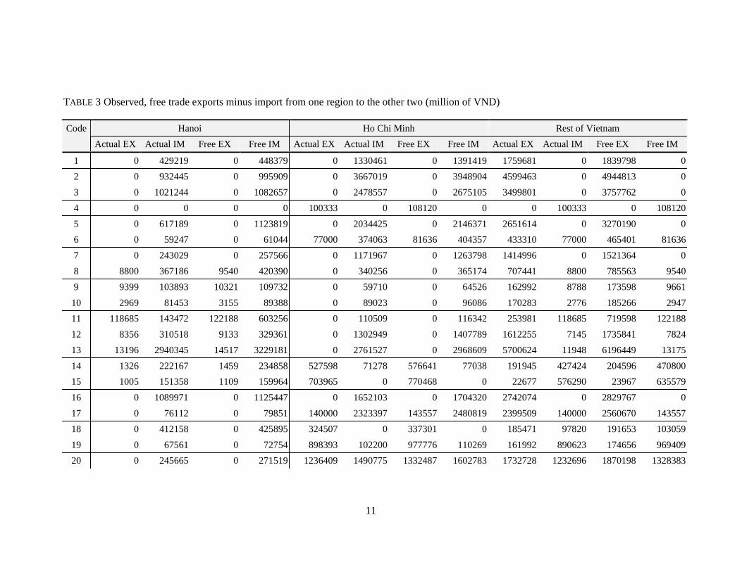
11

TABLE 3 Observed, free trade exports minus import from one region to the other two (million of VND)

Hanoi Ho Chi Minh Rest of Vietnam Code

Actual EX Actual IM Free EX Free IM Actual EX Actual IM Free EX Free IM Actual EX Actual IM Free EX Free IM

1 0 429219 0 448379 0 1330461 0 1391419 1759681 0 1839798 0

2 0 932445 0 995909 0 3667019 0 3948904 4599463 0 4944813 0

3 0 1021244 0 1082657 0 2478557 0 2675105 3499801 0 3757762 0

4 0 0 0 0 100333 0 108120 0 0 100333 0 108120

5 0 617189 0 1123819 0 2034425 0 2146371 2651614 0 3270190 0

6 0 59247 0 61044 77000 374063 81636 404357 433310 77000 465401 81636

7 0 243029 0 257566 0 1171967 0 1263798 1414996 0 1521364 0

8 8800 367186 9540 420390 0 340256 0 365174 707441 8800 785563 9540

9 9399 103893 10321 109732 0 59710 0 64526 162992 8788 173598 9661

10 2969 81453 3155 89388 0 89023 0 96086 170283 2776 185266 2947

11 118685 143472 122188 603256 0 110509 0 116342 253981 118685 719598 122188

12 8356 310518 9133 329361 0 1302949 0 1407789 1612255 7145 1735841 7824

13 13196 2940345 14517 3229181 0 2761527 0 2968609 5700624 11948 6196449 13175

14 1326 222167 1459 234858 527598 71278 576641 77038 191945 427424 204596 470800

15 1005 151358 1109 159964 703965 0 770468 0 22677 576290 23967 635579

16 0 1089971 0 1125447 0 1652103 0 1704320 2742074 0 2829767 0

17 0 76112 0 79851 140000 2323397 143557 2480819 2399509 140000 2560670 143557

18 0 412158 0 425895 324507 0 337301 0 185471 97820 191653 103059

19 0 67561 0 72754 898393 102200 977776 110269 161992 890623 174656 969409

20 0 245665 0 271519 1236409 1490775 1332487 1602783 1732728 1232696 1870198 1328383

12

21 141184 0 151150 0 0 819710 0 876527 814399 135873 870847 145470

22 188340 0 201968 0 1418244 0 1520865 0 0 1606584 0 1722833

23 0 438878 0 463617 150000 543304 158672 588389 836900 4718 898534 5200

24 376773 0 404432 0 1876434 0 2014183 0 0 2253207 0 2418615

25 844957 0 918388 0 1513 568168 1645 613537 538770 817072 581791 888288

26 66416 0 70638 0 0 521488 0 559626 521488 66416 559626 70638

27 243056 0 263036 0 4508790 703000 4879434 757024 703000 4751846 757024 5142470

28 1038833 0 1117331 0 150000 872067 161408 931896 803788 1120554 858933 1205776

29 1341275 0 1467390 0 235284 0 257407 0 0 1576559 0 1724797

30 487752 0 533439 0 78000 368024 85347 396597 352636 550364 380014 602203

31 3264438 0 3525679 0 0 1451044 0 1559506 1243080 3056474 1335998 3302171

32 132906 0 141980 0 15000 0 16024 0 0 147906 0 158004

33 0 317370 0 338373 200000 1213239 213300 1296479 1338844 8235 1430397 8845

34 0 204417 0 221738 0 2996130 0 3216769 3200547 0 3438508 0

35 0 18322 0 19603 321896 80291 342581 86427 83264 306547 89608 326159

36 1622584 0 1795680 0 0 0 0 0 0 1622584 0 1795680

37 1710620 0 1843331 0 3329545 0 3587852 0 0 5040165 0 5431183

38 365043 0 393994 0 19222 0 20746 0 0 384265 0 414741

39 1516257 0 1639910 0 0 0 0 0 0 1516257 0 1639910

40 2112864 0 2206912 0 299284 4000 312606 4297 4000 2412148 4297 2519518

41 1094494 0 1165605 0 3393823 273528 3611803 292941 153003 4367792 163862 4648329

42 1152374 0 1273645 0 5462300 44072 6037130 47654 44072 6614674 47654 7310776

43 1602920 0 1761627 0 2419926 0 2659525 0 0 4022846 0 4421152

44 904384 0 994734 0 0 1093027 0 1180984 960645 772002 1037949 851699

13

TABLE 4 Gross output gained from free trade for Hanoi, Ho Chi Minh and the rest of

Vietnam (million of VND)

Hanoi Ho Chi Minh Rest of Vietnam

Observed Free Observed Free Observed Free

c 1.0000 1.0541 1.0000 1.0810 1.0000 1.1067

Gross

output 65,317,627 72,540,703 160,641,147 171,520,938 722,382,986 768,128,922

Table 4 presents gain from free trade. Perfect competition and free trade would boost

the Hanoi, Ho Chi Minh and Rest of Vietnam economy (activity level of domestic

final demand) by 5.4%, 8.1% and 10.7% respectively. Consequently, gross output

would increase. The difference reflects the relative importance of inter-regional trade

of the three economies. Gains are obtained by elimination of the domestic waste of

resources from misallocation and less than full utilization of resources.

4. Discussion of the Model

No scenario is tested about the shift of comparative advantages of free access to the

technology (such as Hanoi and Ho Chi Minh using Rest of Vietnam technology). The

shift in this scenario might be a good explanation for the location of production. It is

particularly noteworthy that one region’s technology is superior in some sectors hence

the technologies then adopted by the other region.

Each region would have three set of activity level, corresponding to three alternative

choices of technology. Activity vector s now will be 1s , 2s and 3s . Concerning the

activity level of domestic final demand c , now we have also three set namely, 1c , 2c

and 3c .

It is note that A can be written as follows:

11 12 13

1 21 22 23

31 32 33

A A A

A A A A

A A A

=

(10)

14

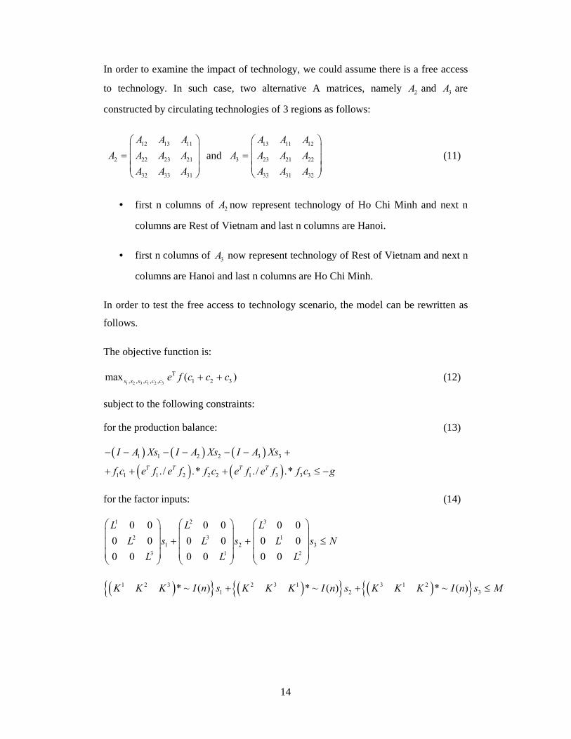
In order to examine the impact of technology, we could assume there is a free access

to technology. In such case, two alternative A matrices, namely 2A and 3A are

constructed by circulating technologies of 3 regions as follows:

12 13 11

2 22 23 21

32 33 31

A A A

A A A A

A A A

=

and 13 11 12

3 23 21 22

33 31 32

A A A

A A A A

A A A

=

(11)

• first n columns of 2A now represent technology of Ho Chi Minh and next n

columns are Rest of Vietnam and last n columns are Hanoi.

• first n columns of 3A now represent technology of Rest of Vietnam and next n

columns are Hanoi and last n columns are Ho Chi Minh.

In order to test the free access to technology scenario, the model can be rewritten as

follows.

The objective function is:

1 2 3 1 2 3, , , , , 1 2 3max ( )s s s c c c e f c c cΤ + + (12)

subject to the following constraints:

for the production balance: (13)

( ) ( ) ( )( ) ( )1 1 2 2 3 3

1 1 1 2 2 2 1 3 3 3. / .* . / .*T T T T

I A Xs I A Xs I A Xs

f c e f e f f c e f e f f c g

− − − − − − +

+ + + ≤ −

for the factor inputs: (14)

1 2 3

2 3 1

1 2 3

3 1 2

0 0 0 0 0 0

0 0 0 0 0 0

0 0 0 0 0 0

L L L

L s L s L s N

L L L

+ + ≤

( ){ } ( ){ } ( ){ }1 2 3 2 3 1 3 1 2

1 2 3* ~ ( ) * ~ ( ) * ~ ( )K K K I n s K K K I n s K K K I n s M+ + ≤

15

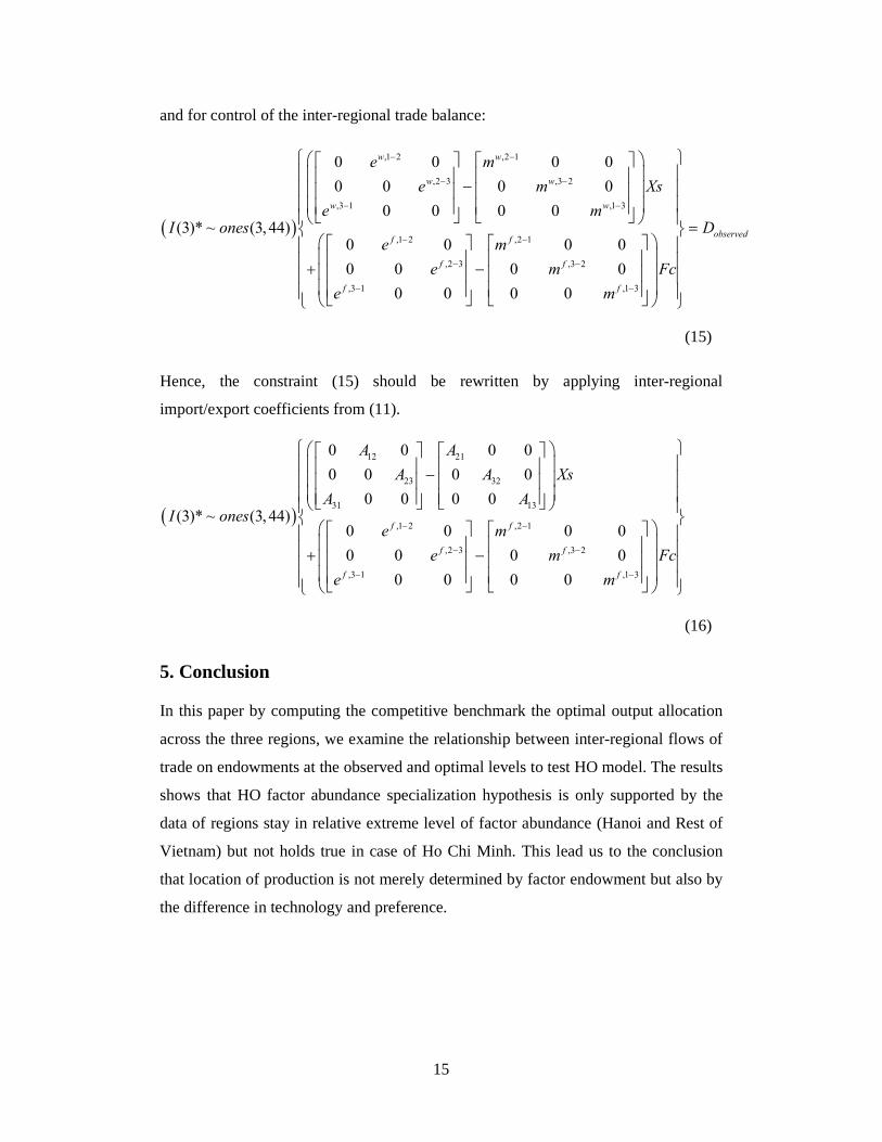
and for control of the inter-regional trade balance:

(15)

Hence, the constraint (15) should be rewritten by applying inter-regional

import/export coefficients from (11).

( )

12 21

23 32

31 13

,1 2 ,2 1

,2 3 ,3 2

,3 1 ,1 3

0 0 0 0

0 0 0 0

0 0 0 0(3)* ~ (3, 44)

0 0 0 0

0 0 0 0

0 0 0 0

f f

f f

f f

A A

A A Xs

A AI ones

e m

e m Fc

e m

− −

− −

− −

−

+ −

(16)

5. Conclusion

In this paper by computing the competitive benchmark the optimal output allocation

across the three regions, we examine the relationship between inter-regional flows of

trade on endowments at the observed and optimal levels to test HO model. The results

shows that HO factor abundance specialization hypothesis is only supported by the

data of regions stay in relative extreme level of factor abundance (Hanoi and Rest of

Vietnam) but not holds true in case of Ho Chi Minh. This lead us to the conclusion

that location of production is not merely determined by factor endowment but also by

the difference in technology and preference.

( )

,1 2 ,2 1

,2 3 ,3 2

,3 1 ,1 3

,1 2 ,2 1

,2 3 ,3 2

,3 1 ,1 3

0 0 0 0

0 0 0 0

0 0 0 0(3)* ~ (3, 44)

0 0 0 0

0 0 0 0

0 0 0 0

w w

w w

w w

f f

f f

f f

e m

e m Xs

e mI ones

e m

e m Fc

e m

− −

− −

− −

− −

− −

− −

− + −

observedD=

16

Reference

Bernstein, J. R. and Weinstein, D. E. (2002). Do endowments predict the location of

production? Evidence from national and international data, Journal of International

Economics, 56, pp. 55–76.

Bowen, H.P., Leamer, E.E., Sveikauskas, L. (1987). Multifactor, multicountry tests of the

factor abundance theory. American Economic Review, 77, pp. 791–809.

Davis, D., Weinstein, D., Bradford, S. and Shinpo, K. (1997) Using international and

Japanese regional data to determine when the factor abundance theory of trade works,

American Economic Review, 87, pp. 421-446.

Kubo Y., Robinson S., Syrquin M. (1986). The Methodology of Multisector Comparative

Analysis. pages 121-147. In Chenery et al (ed.). Industrialization and Growth A

Comparative Study. New York: Oxford University Press.

Ngoc, Q. P. (2007). On the measure of forward and backward linkage. Depocen Working

Paper Series 0704.

Sikdar, C., ten Raa, T., Mohnen, P., Chakraborty, D. (2006). Bilateral Trade between India

and Bangladesh: A General Equilibrium Approach, Economic System Research, 18

(3), pp. 257-279.

Ten Raa, T. and Mohnen, P. (2001), The Location of Comparative Advantages on the Basis

of Fundamentals Only, Economic System Research, 13 (1), pp. 93-108.

Ten Raa, T. and Mohnen, P. (2002), Neoclassical Growth Accounting and Frontier Analysis:

A Synthesis, Journal of Productivity Analysis, 18, pp.111-128.

Trefler, D. (1993). International factor price differences: Leontief was right!. Journal of

Political Economy, 101, pp. 961–987.

Trefler, D. (1995). The case of the missing trade and other mysteries. American Economic

Review, 85, pp. 1029–1046.

17

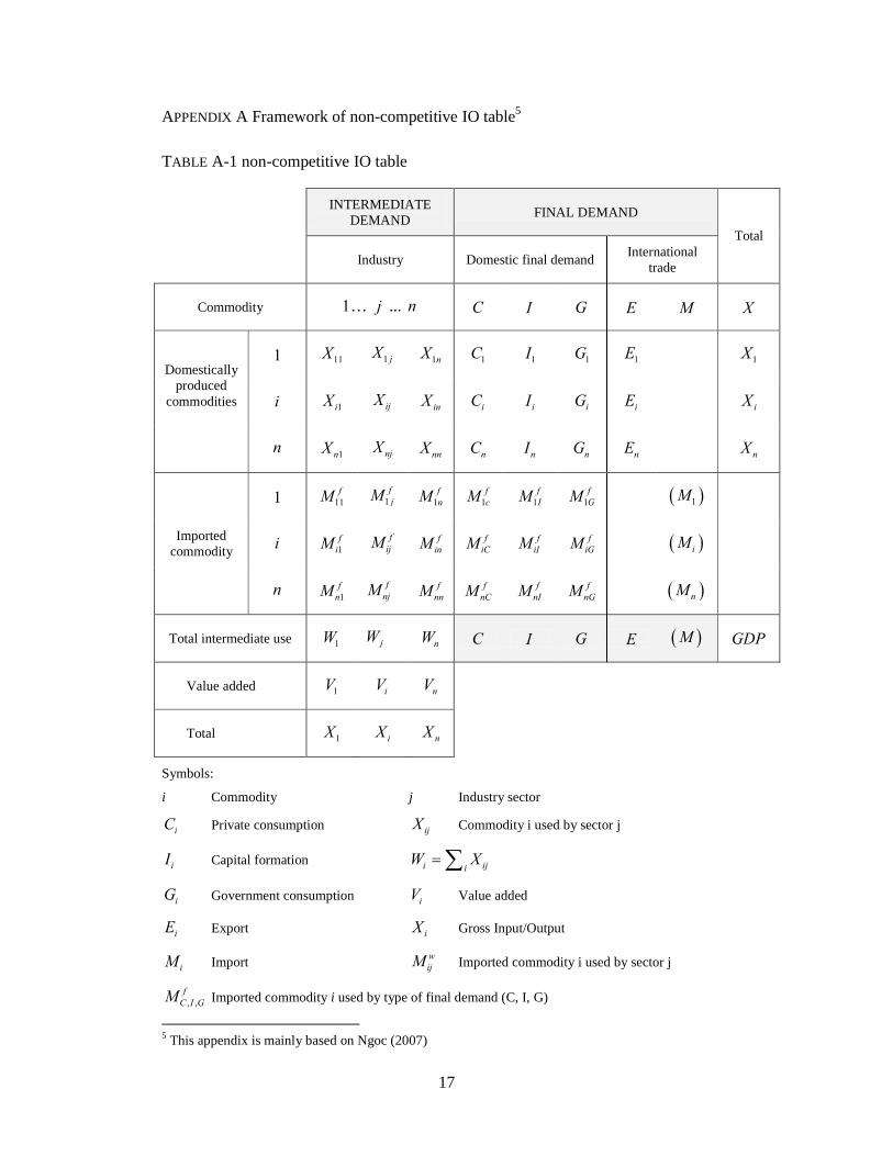
APPENDIX A Framework of non-competitive IO table5

TABLE A-1 non-competitive IO table

INTERMEDIATE

DEMAND FINAL DEMAND

Industry Domestic final demand International

trade

Total

Commodity 1… j ... n C I G E M X

1 11X 1 jX

1nX 1C 1I 1G 1E 1X

i 1iX ijX inX iC iI iG iE iX

Domestically produced

commodities

n

1nX njX nnX nC nI nG nE nX

1 11

fM 1

f

jM 1

f

nM 1

f

cM 1

f

IM 1

f

GM ( )1M

i 1

f

iM f

ijM f

inM f

iCM f

iIM f

iGM ( )iM Imported

commodity

n 1

f

nM f

njM f

nnM f

nCM f

nIM f

nGM ( )nM

Total intermediate use 1W jW nW C I G E ( )M GDP

Value added 1V iV nV

Total 1X iX nX

Symbols:

i Commodity j Industry sector

iC Private consumption ijX Commodity i used by sector j

iI Capital formation i iji

W X=∑

iG Government consumption iV Value added

iE Export iX Gross Input/Output

iM Import w

ijM Imported commodity i used by sector j

, ,

f

C I GM Imported commodity i used by type of final demand (C, I, G)

5 This appendix is mainly based on Ngoc (2007)

18

Table A-1 shows the sample of non-competitive type IO table. The disadvantages of

using competitive type IO table is that we have to assume that all intermediate

demand are satisfied by domestically produced commodities and goods are imported

only for satisfying final demand. This assumption is no-longer hold in the non-

competitive type IO. The starting point for derivation of non-competitive IO tables is

the material balance equation of the input-output account:

i i i i iX W D E M= + + − (A.1)

where:

iX = gross output of sector i

iW = intermediate domestic demand for the output of sector i 1

iD = domestic demand final of product i

iE = export demand of product i

iM = total import of commodity classified in sector i

Import of commodity i, iM , consists of wM for intermediate demand and fM for

final demand. They appear in the total import supply and as part of both intermediate

and final demand in equation (A.1). Let wiu and f

iu stand for the domestic supply

ratios (the proportion of intermediate and of final demand produced domestically).

Hence we have:

w f

i i ij j i i ijX u a X u D E= + +∑ (A.2)

w f

i i i i iM m W m D= + (A.3)

where the import coefficients are define as ( )1i i

m u= − for both intermediate and

final goods.

According to Kubo et al (1986), we assume that: first, there is no direct re-export of

imports; second, imports and domestic goods with the same sector classification are

alternative sources of supply and are perfect substitutes in all uses; third, the domestic

supply ratio for intermediate use, wiu , is assumed to be same for all sectors using

commodity i as an input.

19

Equation (2) and (3) can be conveniently restated in matrix notation as:

ˆ ˆw fX u AX u D E= + + (A.4)

ˆ ˆw fM m AX m D= + (A.5)

In this study, however, it was imperative that a national imports table be generated

that could adequately serve as the basis in regionalizing the import transaction. For

this purpose, a direct estimation methodology was developed to build the import

coefficient matrices. The approximation of diagonal matrix of import coefficients for

intermediate use ̂wm can be calculated as follows:

The import coefficient of sector i, ˆ wiim , can be estimated by the equation:

ˆ w i

ii

i

Mm

TDD= (A.6)

where iTDD is total domestic demand for sector i 6.

Equation (A.1) can be conveniently rewritten in matrix notation as:

1 1( ) ( ) ( )X I A D E M I A Y− −= − + − = − (A.7)

where:

Y D E M= + − Total domestic final demand (excluding imports)

A Direct input coefficient matrix and represents the technology of

inter-industry relations. A consists of two components: the

domestic component and the imported one.

A can be written as follows:

d mA A A= + (A.8)

where:

d wA u A=⌢

domestic direct input/output coefficient matrix

m wA m A=

⌢

import coefficient matrix for intermediate use

6 By definition

TDD

i=W

i+ D

i= X

i− E

i+ M

i (which is can be calculated with the data can be

extracted from competitive IO table).

20

Replace d wA u A=⌢

, equation (A.4) can be rewritten as follows:

ˆd fX A X u D E= + + (A.9)

Hence we have:

1 ˆ(1 ) ( )d fX A u D E−= − + (A.10)

Equation (A.10) shows the new material balance of the non-competitive type input-

output table. They show that in an economy, a part of intermediate demand and final

demand (including export) are satisfied by all domestically produced commodities.

Compared to the original material balance described by (A.1), advantage of using

non-competitive type IO is that in its material balance there is no appearance of

imported commodities. Hence material balance accounts are not been biased by

assume that all intermediate demand are satisfied by domestically produced

commodities and goods are imported only for satisfying final demand.

21

APPENDIX B Data

The study requires data complied from several sources.

In order to test theories of interregional trade we use inter-regional input-output

(IRIO) data and factor endowments of Vietnam in 2000: the inter-regional input-

output (IRIO) table of Hanoi, Ho Chi Minh and rest of Vietnam 2000 was compiled

by the author in corporation with research team from General Statistic Office of

Vietnam (GSO of Vietnam). Data required for the compilation of these IRIO table

are: national input-output table of 2000 is published by GSO of Vietnam; input-output

tables of Ho Chi Minh and Hanoi in 2000 is unpublished, compiled research team

from GSO of Vietnam; inter-regional trade data in 2000 is published by GSO of

Vietnam.

Labor and capital stock data are taken from the enterprise census 2000 which is

published by GSO of Vietnam. The data on capacity utilization are from the

Statistical Year Books published by the General Statistic Office (GSO) of Vietnam in

2000.

Table B-1 presents the description of IRIO table used in this study.

Symbols:

i Commodity j Industry sector

C Consumption CF Capital formation

EX Exports IM Imports

HCM Ho Chi Minh ROV Rest of Vietnam

ID Intermediate demand FD Final demand

VA Value added GI Gross input

Produc-Tax Tax on production Op.Surplus Operating surplus

22

TABLE B-1 IRIO table of Hanoi, Ho Chi Minh and Rest of Vietnam

INTERMEDIATE DEMAND FINAL DEMAND

Hanoi HCM ROV Hanoi HCM ROV

1 … j … n 1 … j … n 1 … j … n C CF EX C CF EX C CF EX

Foreign Import

Total Gross Output

1 0 : : i 0 : : H

anoi

n

Hanoi commodities consumed by

Hanoi industries

Hanoi commodities consumed by

HCM industries

Hanoi commodities consumed by

ROV industries

Hanoi commodities consumed by

Hanoi Final Demand

Hanoi commodities consumed by

HCM Final Demand

Hanoi commodities consumed by

ROV Final Demand 0 H

anoi

Gro

ss

Out

put

1 0 : : i 0 : : H

CM

n

HCM commodities consumed by

Hanoi industries

HCM commodities consumed by

HCM industries

HCM commodities consumed by

ROV industries

HCM commodities consumed by

Hanoi Final Demand

HCM commodities consumed by

HCM Final Demand

HCM commodities consumed by

ROV Final Demand 0 H

CM

Gro

ss

Out

put

1 0 : : i 0 : : R

OV

n

ROV commodities consumed by

Hanoi industries

ROV commodities consumed by

HCM industries

ROV commodities consumed by

ROV industries

ROV commodities consumed by

Hanoi Final Demand

ROV commodities consumed by

HCM Final Demand

ROV commodities consumed by

ROV Final Demand 0 R

OV

Gro

ss

Out

put

1 : i :

Res

t of

Wor

ld

n

Imported commodities consumed by

Hanoi industries

Imported commodities consumed by

HCM industries

Imported commodities consumed by

ROV industries

Imported commodities consumed by

Hanoi Final Demand

Imported commodities consumed by

HCM Final Demand

Imported commodities consumed by

ROV Final Demand

(FIM

)

Total Hanoi ID HCM ID ROV ID Hanoi FD HCM FD ROV FD

Wages Produc-Tax Op.Surplus

Depreciation Total VA Hanoi VA HCM VA ROV VA Total GI Hanoi GI HCM GI ROV GI

23

APPENDIX C Sectoral code

Code Description

1 Paddy 2 Other crops 3 Livestock and poultry 4 Agricultural services 5 Fishery 6 Forestry 7 Mining and quarrying 8 Processed, preserved meat, animal oils and fats 9 Milk, butter & other dairy products 10 Processed, preserved fruits and vegetable products 11 Processed seafood and by products 12 Sugar (all kinds), coffee and tea, processed 13 Rice, processed and other food manufactures 14 Alcohol, beer and liquors, non-alcohol water and soft drinks 15 Cigarettes and other tobacco products 16 Textiles 17 Garment 18 Manufacture of leather tanneries 19 Processed wood and wood products 20 Paper pulp and paper products Printing and publishing 21 Basic chemicals and by-products; petroleum products 22 Fertilizer, pesticides, veterinary 23 Health medicine 24 Processed rubber and by products, plastic and by-products 25 Non-metallic mineral products 26 Ferrous metals and products 27 Non-ferrous metals and products 28 General & special-purpose machinery; office, accounting & computing machines 29 Electrical machinery and equipment 30 Home appliances and its spare parts 31 Motor vehicles, transport means and spare parts 32 Health instruments, precise equipment & apparatus 33 Other manufactured products 34 Electricity and gas 35 Water and water supply 36 Construction 37 Trade 38 Passenger transport services 39 Goods transport services 40 Communication services 41 Financial services, insurance, real estate, business services, science & technology 42 State management, defence and compulsory social security Education and training;

health care; culture and sport 43 Hotels, restaurants 44 Other services, not elsewhere classified