Embed Size (px)
Citation preview
FACTOR AUGMENTED AUTOREGRESSIVE DISTRIBUTED LAG MODELSWITH MACROECONOMIC APPLICATIONS
Dalibor Stevanovic ∗
First version: November 2014This version: June 21, 2015
Abstract
This paper proposes a factor augmented autoregressive distributed lag (FADL) frameworkfor analyzing the dynamic effects of common and idiosyncratic shocks. We first estimate thecommon shocks from a large panel of data with a strong factor structure. Impulse responsesare then obtained from an autoregression, augmented with a distributed lag of the estimatedcommon shocks. The approach has three distinctive features. First, identification restrictions,especially those based on recursive or block recursive ordering, are very easy to impose. Second,the dynamic response to the common shocks can be constructed for variables not necessarilyin the panel. Third, the restrictions imposed by the factor model can be tested. The relationto other identification schemes used in the FAVAR literature is discussed. The methodology isused to study the effects of monetary policy and news shocks.
JEL Classification: C32, E17
Keywords: Factor Models, Structural VAR, Impulse Response
∗Departement des sciences economiques, Universite du Quebec a Montreal. 315, Ste-Catherine Est, Montreal,QC, H2X 3X2. ([email protected])I am very grateful to Serena Ng for her guidance and a large number of discussions from the very beginning of thisproject. The author acknowledges financial support from the Fonds de recherche sur la societe et la culture (Quebec).

1 Introduction
This paper proposes a new approach for analyzing the dynamic effects of q common shocks such as
due to monetary policy and technology on q or more observables. We assume that a large panel of
data XALL = (X,XOTH) is available and use the sub-panel X that is likely to have a strong factor
structure to estimate the common shocks. Identification is based on restrictions on a q dimensional
subset of X or on q block specific dynamic shocks. The impulse response coefficients are obtained
from an autoregression in each variable of interest augmented with current and lagged values of
the identified common shocks. Observed factors can coexist with latent factors. We refer to this
approach as Factor Augmented Autoregressive Distributed Lag (FADL).
An important feature of the FADL is that it estimates the impulse responses using minimal
restrictions from the factor model. The approach has several advantages. First, while X is large in
dimension, identification is based on a subset of variables whose dimension is the number of common
shocks. This reduces the impact of invalid restrictions on variables that are not of direct interest.
Second, the impulse responses are the coefficients estimated from a regression with common shocks
as predictors. Additional restrictions are easy to impose, and for many problems the impulse
responses can be estimated on an equation by equation basis. Third, the analysis only requires
a strong factor structure to hold in X and is less likely to be affected by the possibility of weak
factors in XOTH .
The proposed FADL methodology lets the data speak whenever possible and is in the spirit of
vector-autoregressions (VAR) proposed by Sims (1980). The FADL also shares some similarities
with the Factor Augmented Vector Autoregressions (FAVAR) considered in Bernanke and Boivin
(2003). Their FAVAR expands the econometrician’s information set without significantly increasing
the dimension of the system. Our FADL further simplifies the analysis by imposing restrictions only
on the variables of interest. Recursive and non-recursive restrictions can be easily implemented.
The FADL is derived from a structural dynamic factor model which has a restricted FAVAR
as its reduced form. A factor model imposes specific assumptions on the covariance structure of
the data. Even though many variables are available for analysis, a factor structure may not be
appropriate for every series. As noted in Boivin and Ng (2006), more data may not be beneficial for
factor analysis if the additional data are noisy and/or do not satisfy the restrictions of the factor
model. We treat X like a training sample. Using it to estimate the common shocks enables us to
validate the factor structure in XOTH , the series not in X.
The FADL approach stands in contrast to structural FAVARs that impose all restrictions of a
dynamic factor model in estimation, as Forni, Giannone, Lippi, and Reichlin (2009). The FADL
estimates will necessarily be less efficient if the restrictions are correct, but are more robust when
the restrictions do not hold universally. As in Stock and Watson (2005), our FADL also permits
implications of the factor model to be tested. However, we go one-step further by letting the data
determine the Wold representation instead of inverting a large FAVAR.
The paper proceeds as follows. Section 2 first sets up the problem of identifying the effects
of common shocks from the perspective of a dynamic factor model. It then presents the FADL
framework without observed factors. Estimation and identification of a FADL is discussed in Section
1
3. Relation of FADL to alternative structural dynamic factor analysis is discussed in Section 4, and
FADL is extended to allow for observed factors. Simulations are presented in Section 5. Section
6 considers the identification of monetary and news shocks and the estimation of their effects on
economic activity. Both examples highlight the main features of FADL: the ability to perform
impulse responses analysis and to test the validity of the factor structure of variables not used in
estimation or identification of the common shocks.
2 Dynamic Factor Models and the FADL Framework
Let N be the number of cross-section units and T be the number of time series observations where
N and T are both large. We observe data XALL = (X, XOTH) which are stationary or have been
transformed to be covariance stationary. It is assumed that Xt = (X1t, . . . , XNt)′ has a (strong)
factor representation and can be decomposed into a common and an idiosyncratic component:
Xt = λ(L)ft + uXt (1)
where ft = (f1t, . . . , fqt)′ is a vector of q common factors and λ(L) = λ0 + λ1L + . . . λsL
s is a
polynomial matrix of factor loadings in which the N × q matrix λj = (λj1 . . . , λjN )′ quantifies
the effect of the common factors at lag j on Xt. In particular, the i-th element of λ(L) consists
of λi(L) = (λi1(L), . . . , λiq(L)), λik(L) =∑pi,k
j=0 λi,k,jLj , where pi,k is the finite lag order of the
k−th factor loadings polynomial of variable i. The series-specific errors uXt = (uX1t, . . . , uXNt)′
are mutually uncorrelated but can be serially correlated. We assume
uXt = D(L)uX,t−1 + vXt (2)
where D(L) is a finite-order N -dimensional matrix poynomial and vXt is a vector white noise
process. The q latent dynamic factors are assumed to be a vector autoregressive process of order
h. Without loss of generality, we assume h = 1 and thus
ft = Γ1ft−1 + Γ0vft (3)
where the characteristic roots of Iq − Γ1L are strictly less than one. The q × 1 vector vft consists
of structural common shocks (such as monetary policy or technology). These structural shocks can
affect several dynamic factors simultaneously. Hence, the q × q matrix Γ0 need not be an identity.
By assumption, E(vXitvXjt) = 0 and E(vXitvfkt) = 0 for all i 6= j and for all i = 1, . . . N and
k = 1, . . . q.
Assuming that I−D(L)L is invertible, the vector-moving average representation of Xt in terms
of the structural common and idiosyncratic shocks is
Xt = Ψf (L)vft + ΨX(L)vXt.
The structural impulse response coefficients ΨXj and Ψf
j are defined from
ΨX(L) =∞∑j=0
ΨXj L
j = (I −D(L)L)−1
Ψf (L) =
∞∑j=0
ΨfjL
j = λ(L)(I − Γ1L)−1Γ0.
2

For each j ≥ 0, Ψfj is a N×q matrix summarizing the effect of a unit increase in vft after j periods.
We use Ψfj,i1:i2,k1:k2 to denote the submatrix in the i1 to i2 rows and k1 to k2 columns of Ψf
j . When
i1 = i2 = i and k1 = k2 = k, we use ψfj,i,k to denote the effect of shock k in period t on series i in
period t+ j.
The objective of the exercise is to uncover the dynamic effects (or the impulse response) of the
structural common shocks vft on variables of interest. By using X1t, . . . , XNt for factor analysis,
the econometrician’s information set is of dimension N . Forni, Giannone, Lippi, and Reichlin
(2009) argue that non-fundamentalness is generic of small scale models but cannot arise in a large
dimensional dynamic factor model. The reason is that Ψf (z) is a rectangular rather than a square
matrix and its rank is less than q for some z only if all q × q sub-matrices of Ψf (z) are singular,
which is highly unlikely. Assuming that N is large ensures that the common shocks are fundamental
for X.
However, even if N is large, nothing distinguishes one common shock from another. In a VAR
analysis with q endogenous variables and q shocks, q(q − 1)/2 restrictions will be necessary. A
popular approach is to impose contemporaneous exclusion restrictions such that a rank condition is
satisfied, see, eg. Deistler (1976), Rubio-Ramırez, Waggoner, and Zha (2010). If the identification
restrictions imply a recursive ordering, then the parameters can be identified sequentially and
estimation can proceed on an equation by equation basis.
While ΨX0 = IN in a dynamic factor model, the contemporaneous response of Xt to common
shocks vft is given by
Ψf0 = λ0Γ0 =
λ0,1,1 λ0,1,2 . . . λ0,1,q...
...
λ0,q,1 λ0,q,2 . . . λ0,q,q...
...
λ0,N,1 λ0,N,2 . . . λ0,N,q
Γ0,1,1 . . . Γ0,1,q...
Γ0,q,1 . . . Γ0,q,q
.
The (i, k) entry of λ0 is the contemporaneous effect of factor k on series i, and the (k, j) entry of Γ0
is the effect of the j-th common shock on factor k. In general, Ψf0 will not be an identity matrix.
Two additional problems make the identification problem non-standard. First, while having
more total shocks than endogenous variables should facilitate identification, the common shocks
also restrict the co-movements across series. Imposing constraints on an isolated number of series
is actually quite difficult within the factor framework. Zero restrictions on the entries of λ0 or Γ0
alone are not usually enough to ensure that a particular entry of Ψf0 takes on the desired value
(often zero). Second, the dynamic factors are themselves latent. Thus, not only do we need to
identify the effects of vf , we also need to identify vf .
Our analysis is based on the following assumptions.
Assumption 1: E(vft) = 0, E(vftv′ft) = Iq.
3

Assumption 2: D(L) is a diagonal matrix with δi(L), a finite px,i-degree lag polynomial, in the
i-th diagonal, i.e.
D(L) =
δ1(L) 0 . . . 0...
......
0 0 . . . δN (L)
,
Assumption 3: For some j, a q × q matrix of Ψfj is full rank.
Assumption 1 is a normalization restriction as we cannot separate the size of the common shocks
from their impact effects. Assumption 2 is a form of exclusion restriction. We assume univariate
autoregressive dynamics for idiosyncratic errors:
uXit = δi(L)uXit−1 + vXit.
This implies that dynamic correlations between any two series are due entirely to the common
factors, which is the defining feature of a dynamic factor model. Diagonality of D(L) in turn
allows Xit to be characterized by an autoregressive distributed lag model with serially uncorrelated
idiosyncratic errors:
Xit = δi(L)Xit−1 + λi(L)ft + vXit, (4)
where λi(L) = (1 − δi(L))λi(L). For simplicity, we assume λi(L) is of order s for all i.1 A
representation that is more useful for impulse response analysis is an autoregressive distributed lag
in the primitive shocks vft:
Xit = δi(L)Xit−1 + ψfi (L)vft + vXit (5)
where
ψfi (L) = (1− δi(L))λi(L)(I − Γ1L)−1Γ0.
We will henceforth refer to (5) as the FADL representation of Xit. Note that (1 − δi(L))−1ψfi (L)
is precisely the i-th row of Ψf (L).2
The dynamic effects of the common shocks vft on Xit are defined by the coefficients ψfi (L).
If vf were observed and N = q, equation (5) defines a dynamic simultaneous equations system in
which identification can be achieved by excluding some vf or its lags from certain equations. For
example, contemporaneous restrictions can be imposed so that the q× q matrix Ψf0 has rank q. As
1In general, λi(L) is a lag polynomial of the maximum order maxk∈1,...,q(pi,k) times pi,x.2In Dufour and Stevanovic (2013) the authors argue that factors’ dynamics obey, in general, a VARMA process.
The FADL representation still holds. Assume an identified VARMA(1,1) process for factors:
ft = Γ1ft−1 + Θ1Γ0vft−1 + Γ0vft.
Then, the FADL representation of Xit is the same as in (5) except that
ψfi (L) = (1 − δi(L))λi(L)(I − Γ1L)−1(I + Θ1)Γ0.
4
our system is tall with N ≥ q, Assumption 3 requires that a q × q submatrix of Ψfj is full rank. If
all restrictions are imposed on Ψf0 , Assumption 3 will hold if the top q × q submatrix of Ψf
0 has
rank q. However, long run and sign restrictions are also permitted.
Assumptions 1 to 3 are fairly standard. But our factors are also latent and we can only identify
the space spanned by the factors and not the factors themselves. To make the procedure operational,
we need to replace vft by estimates vft which have the same properties as Assumption 1. These
identification conditions will be further developed below.
3 Estimation and Identification
If there are q common shocks, we will need at least q series for identification. Without loss of
generality, let Yt be the first q series in Xt. Since each yt ⊂ Yt admits a dynamic factor structure,
it holds that
yt = α∗yy(L)yt−1 + α∗yf (L)vft + v∗yt, (6)
where α∗yy(L) and α∗yf (L) are the autoregressive and distributed lag coefficients of the non feasible
regression since the common shocks vft are, in general, not observable. Our impulse response
analysis is rather based on least squares estimation of the FADL
yt = αyy(L)yt−1 + αyf (L)vft + vyt (7)
where a prior restrictions are be imposed on αyf (L) for identification. We now explain how vft is
estimated and how restrictions are imposed on the FADL.
Let Λ be the N × r matrix of loadings, Ft be a r = q(s+ 1)× 1 vector of static factors, where
Λ =
Λ1
Λ2...
ΛN
, Ft =
ftft−1
...ft−s
, ΦF =
Γ1 Γ2 . . . ΓsIq 0 . 0 . 00 Iq 0 . 0. 0 . . 00 0 . Iq . 0
Λi =(λi0 λi1 . . . λis
).
Note that we have assumed a VAR(1) process for dynamic factors. Despite it implies a particular
structure for Ft and ΨF , there is no loss of generality.3 The starting point is the static factor
representation of the pre-whitened data, xit = (1− δi(L)L)Xit:
xit = ΛiFt + vXit (8)
Ft = ΦFFt−1 + εFt (9)
εFt = Gεft. (10)
3Bai and Ng (2007) show that the vector of static factors, Ft, is of dimension r = q(s+ 1) × 1 and follows a VARof order depending on h and s. For instance, if ft follows a finite-order VAR(h), then Ft = (f ′t , f
′t−1, . . . , f
′t−max(h,s))
′
follows a VAR with
ΦF =
Γ1 Γ2 . . . Γmax(h,s)+1
Iq 0 . 0 . 00 Iq 0 . 0. 0 . . 00 0 . Iq . 0
where Γh+1 = . . . = Γmax(h,s)+1 = 0.
5

The εFt are the reduced form errors of Ft and are themselves linear combinations of the structural
shocks vft and εft = Γ0vft is the vector of reduced form common shocks, see (3). The r× q matrix
G maps the structural dynamic shocks to the reduced form static shocks. Since Xt is assumed to
have a strong factor structure, Λ′Λ/N → Λ > 0 as N → ∞, and the N × N matrix 1T
∑Tt=1 xtx
′t
has r eigenvalues that diverge as N,T → ∞ while the largest eigenvalue of the N ×N covariance
matrix of vXt is bounded.
From vXit = xit − ΛiFt = xit − Λi(ΦFFt−1 + εFt), define
εXit = xit − ΛiΦFFt−1
= ΛiεFt + vXit. (11)
As noted in Stock and Watson (2005), the rank of the r × 1 vector εFt is only q, since Ft is
generated by q common shocks. In other words, εXit itself has a factor structure with common
factors εft. But εft are themselves linear combinations of vft. Let
vft = Bεft,
where in principle B = Γ−10 (if Γ−1
0 exists). The q × q matrix B maps the reduced form dynamic
shocks to the structural dynamic shocks. The objective is to identify vft and to trace out its effects
on the variables of interest. If there are q common shocks, q(q − 1)/2 restrictions are necessary to
identify vft via B.
Estimation proceeds in five steps.
Step E1: Estimate Ft from the full panel of data Xt by iterative principal components (IPC).
(i) Initialize δi(L) using estimates from a univariate AR(px,i) regression in Xit. Let D(L) be a
diagonal matrix with δi(L) on the i-th diagonal.
(ii) Iterate until convergence
minD(L),Λ,F
SSR =T∑t=1
((I −D(L)L)Xt − ΛFt
)′((I −D(L)L)Xt − ΛFt
).
(a) Let Ft be the first k principal components of xx′ using the normalization that F ′F/T =
Ik, where x is the T × N matrix of data, F = (F1, F2, . . . , FT )′ and k is the assumed
number of static factors.
(b) Estimate D(L) and Λ by regressing Xit on Ft and lags of Xit.
The method of principal components (PC) estimates k factors as the eigenvectors corresponding
to the k largest eigenvalues of XX ′/(NT ). Under the assumption of strong factors, Bai and Ng
(2006) show that the estimates are consistent for the space spanned by the true factors in the
sense that 1T
∑Tt=1
∥∥∥Ft −HFt∥∥∥2= Op(min(N,T )), where H is a k × r matrix of rank r. However,
the idiosyncratic errors may not be white noise. Stock and Watson (2005) suggest using IPC to
iteratively update δi(L), which is then used to define xit. The static factors form the common
component of xit.
6

Step E2: Estimating the space spanned by vft Estimate a VAR in Ft to obtain ΦF and
εFt and let εXit = xit − Λ′iΦF Ft−1, where Λ and Ft−1, ΦF are obtained from Step (E1). Amengual
and Watson (2007) show that the q principal components of εXt can precisely estimate the space
spanned by εft = Γ0vft. An alternative is to proceed directly from the factors’ VAR residuals εFt.
Bai and Ng (2007) show that q eigenvectors of E(εFtε′Ft) consistently estimate the space spanned
by εft, hence vft. In particular, 1T
∑Tt=1 ‖εft − JNT εft‖ = Op(C
−1NT ), where JNT is a q× q full rank
matrix and CNT = min(√N,√T ).
Step E3: Identification of vft: The columns of common shocks εft are not, in general, inter-
pretable. We seek a matrix B such that
vft = B εft, (12)
and vft is a vector of mutually uncorrelated structural common shocks. The rotation matrix B
differs from B because εft consistently estimates the space spanned by εft, but not each columns
separately. We consider two approaches. The first condition (abbreviated as RO) is lower trian-
gularity of a q × q sub-matrix so that the shocks can be identified recursively from q equations.
The second condition (abbreviated as BO) requires organizing the data into blocks using a priori
information so that the factors estimated from each block can be given meaningful interpretation.
Assumption: Recursive Ordering (RO) Method (RO) is based on an assumed causal struc-
ture in short or in the long run. Just like a VAR, this would require knowledge of which of the q
variables to order recursively in Yt. For j = 1 : q consider estimating the regression:
ytj = ayy,j(L)yt−1,j +
q∑k=1
ayf,j,k(L)εfkt + vyt,j (13)
where εft are the q principal components of the N residuals eXt or q eigenvectors of E(εFtε′Ft). Re-
mark that we specify different autoregressive and distributed lag coefficients from FADL regression
(7) since it contains εft and not vft. The short run zero restrictions can be imposed as follows:
i Let Af0 be the estimated contemporaneous response to the q reduced-form shocks εft:
Af0 =
ayf,0,1,1 ayf,0,1,2 . . . ayf,0,1,q...
......
ayf,0,q,1 ayf,0,q,2 . . . ayf,0,q,q
.
ii Define the q × q matrix B = [chol(Af0A′f0)]−1Af0. Now let
vft = Bεft
αyf,j = ayf,j(L)B−1 j = 1, . . . , q.
7

The long run zero restrictions are imposed through similar steps. For notation purposes, let
ayy(L) = diag[ayy,j(L)], for j = 1, . . . , q, be the diagonal matrix polynomial of the autoregressive
terms in FADL representation (13), and
ayf (L) =
ayf,1,1(L) ayf,1,2(L) . . . ayf,1,q(L)...
......
ayf,q,1(L) ayf,q,2(L) . . . ayf,q,q(L)
be the matrix polynomial of the distributed lag coefficients.
i. Let Af1 be the estimated long run response to the q unorthogonalized shocks εft:
Af1 = (I − ayy(1))−1ayf (1).
ii. Define the q × q matrix B = [chol(Af1A′f1)]−1Af1. Now let
vft = Bεft
αyf,j = ayf,j(L)B−1.
By construction, vft is orthonormal. The method achieves exact identification by using the
causal ordering of the q variables selected for analysis. Hence, the identified impact (long-run)
matrix on q series in yt is lower triangular.
Imposing a causal structure through the ordering of variables is the most common way to
achieve identification of FAVAR. Stock and Watson (2005) also use Assumption RO to identify the
primitive shocks. Their implementation differs from ours in that we apply Choleski decomposition
to the FADL estimates of αyf (0) and hence we do not impose all the restrictions of the factor
model. In contrast, Stock and Watson (2005) impose restrictions implied by the FAVAR in Xt and
Ft. The results are likely to be more sensitive to the choice of Xt.
Assumption Block Ordering (BO) Method (BO) is useful when the data can be organized
into blocks. Let X = (X1, X2, . . . Xq) be data organized into q blocks. To see how data blocks
facilitate identification, observe that the factor estimates ε0ft are linear combinations of εXt. Let
ε0f = εXζ
0 be the T × q matrix of factor estimates where for each t,
ε0ft =
ζ0
11 ζ012 . . . . . . ζ0
1N
ζ021 ζ0
22 . . . . . . ζ02N
......
......
...ζ0q1 ζ0
q2 . . . . . . ζ0qN
εX1t
εX2t...
εXNt
. (14)
Identification requires a priori information on the ζ.
i. For b = 1, . . . q, let εbf be the matrix of eigenvector corresponding to the largest eigenvalues
of the nb × nb matrix εb′X εbX .
ii. Let B be the Choleski decomposition of the q× q sample covariance of εft. Then vft = Bεft.
8
The identification strategy can be understood as follows. From (11), we see that εXt =(ε1′Xt ε2′
Xt . . . εq′Xt)′
have εft as common factors. Since the factors are pervasive by definition,
the factors are also common to all εbXt for arbitrary b. Thus for each b = 1, . . . q, consider a factor
model for εbXit = Λbiεbft + vbXit. If εbXit were observed, the factors for block b can be estimated by
principal components which are linear combinations of series in εbXt. We do not observe εbXt, but
we have εXt = xt− ΛΦF Ft−1 from Step (E2). For example, if X1 is a T ×N1 panel of employment
data, the first principal component of ε1′X ε
1X is a labor market factor εf1t, and if X2 is a panel of
price data, εf2t is a price factor. Collecting the factors estimating from all blocks into εft, we have
εft =
ζ1
1,1:N10 0 . . . 0 0
0 ζ21,1:N2
0 . . . 0 0... 0
......
...0 0 0 . . . 0 ζq1,1:Nq
ε1Xt
ε2Xt...εqXt
(15)
Obviously, the factors are defined by assuming a structured covariance relation in the observables.
The appeal is that we can now associate the q factors with the block of variables from which
they are estimated. However, these factors can still be correlated across blocks. To orthogonalize
them, step (ii) performs q regressions beginning with vf1 = ε1f . For m = 2, . . . q, vfb = Mbε
bf
are the residuals from projecting εbf onto the space orthogonal to vf1, . . . , vf,b−1, and Mb is the
corresponding projection matrix.
Bernanke, Boivin, and Eliasz (2005) treat the interest rate as an observed factor, organize the
macro variables into a fast and a slow block, and estimate the one factor from the slow variables.
Their identification is based on a Choleski decomposition of the residuals in the slow variables and
the observed factor. Their implementation is specific to the question under investigation while our
methodology is general. Our identification algorithm is generic, provided blocks of variables with
meaningful interpretation can be defined.4
In conventional VAR models, the structural impulse responses are obtained by rotating the
reduced form impulse response matrix by a matrix, say, B. The primitive shocks are then obtained
by rotating the reduced form errors with the inverse of the same matrix. In our setup, identification
of structural common shocks precedes estimation of the impulse responses. This allows us to impose
additional economic restrictions on the impulse response functions without simultaneously affecting
the structural shocks. We only presented Wold causal identification structures. However, medium
run (a la Barsky and Sims (2011)) and sign restrictions can be imposed.
Step E4: Constructing Impulse Response Functions: Given identified vft from the previous
step, estimate a univariate FADL by OLS:
yt = αyy(L)yt−1 + αyf (L)vft + vyt (16)
where αyy(L) is a polynomial of order py, and αyf is of order pf . These polynomial orders can be
jointly estimated by Akaike or Bayesian information criteria. The estimated responses of yt to a
4Moench and Ng (2011) construct regional factors from data organized geographically. Ludvigson and Ng (2009)study the relative importance of the factor loadings and find that factor one loads heavily on real activity series,factor two on money and credit variables, while factor three loads on price variables.
9

unit increase in the common shocks vft and idiosyncratic shocks vyt are defined by
ψfy (L) =αyf (L)
1− αyy(L)Lψyy(L) =
1
1− αyy(L)L.
Since αyy(L) is a scalar rational polynomial, the impulse responses are easy to compute using
the filter command in matlab. The least squares estimates [αyy(L), αyf (L)] converge to the
least squares estimates from the infeasible regression (6), [α∗yy(L), α∗yf (L)]. As shown in Step E2,
εft consistently estimates the space spanned by εft, thus regression augmented with εft can be
treated as though εft is observed, see Bai and Ng (2006). However, that regression would produce
unorthogonalized impulse responses and a priori restrictions in form of B = Γ−10 J−1
NT are needed to
obtain ψfy (L). The formal proof is in the Appendix.
Note that by Assumption 1, the standard deviation of all common shocks are normalized to
unity. The response to a unit shock is thus the same as the response to a standard deviation shock.
Note that given interpretation of vft identified from Step E3, additional economic restrictions on
the impulse responses can be directly imposed on αyf for any variable yt being in Yt, Xt or XOTHt .
For example, suppose we have a strong (a priori) reason that a particular (sectoral) total factor
productivity (TFP) series does not react to a technology news shock even at one period lag. This
implies restricting αyf,0,k = αyf,1,k = 0 where k reflects the news shock in vft. Hence, it restricts
the response of that particular variable without affecting the identification of common shocks nor
the estimation of the impulse responses of other series in the system. Moreover, one could produce
impulse responses directly by adapting (16) to local projections as in Jorda (2005).
Step E5: Model Validation Our maintained assumptions are that Ft are pervasive amongst
Xt rather than (Xt, XOTHt ) and by assumption, Xt have a strong factor structure. We refer to X
as a ’training sample’. This is useful because once the estimated common shocks vft are available,
they can be treated as regressors in a FADL model for zt (scalar) not necessarily in Xt. This is
because if (Xt, XOTHt ) have a factor structure, the shocks vft common to Xt are also common to
variables in XOTHt . If the common factors are important for zt ⊂ XOTH
t , then FADL coefficients
on vft and its lags should be statistically significant.
4 Relation to the Other Methods and Allowing for Observed Factors
An important difference between our approach and existing structural FAVAR analysis is that we
estimate the impulse responses directly rather than inverting a VAR. Chang and Sakata (2007)
estimates the shocks as residuals from long vector autoregressions in observed variables. The
authors show that their estimated impulse responses are asymptotically equivalent to the local
projections method used in Jorda (2005). Dufour and Renault (1998) have proposed the local
projections to study the Granger-causality at different horizons. Feve and Guay (2009) develops
similar SVAR framework to study the effects of news shocks on worked hours. Our analysis has the
additional complication that the factors are latent. Thus, we first estimate the space spanned by
common factors, then estimate the space spanned by the common shocks, before finally estimating
the impulse response functions.
10

It is useful to relate our estimate of Ψf (L) with the conventional FAVAR approach which starts
with the representation(FtXt
)=
(Φ 0
ΛΦ D(L)
)(Ft−1
Xt−1
)+
(εFt
ΛεFt + vXt
)from which it follows that
xt = ΛΦL(I − ΦL)−1εFt + ΛεFt + vXt
=
(ΛΦL(I − ΦL)−1 + Λ
)εFt + vXt.
The dynamic effects of shocks εFt to the static factors on (prewhitened) data are determined by
Λ
(ΦL(I − ΦL)−1 + I
)= Λ
∞∑j=0
Φi+1Li+1. (17)
At lag j, the N ×N response matrix
ΛΦj =(
Λ′i Λ′2... Λ′N
)′Φj .
Intuitively, the total effect of εFt depends on Xt through Ft and hence depends on the dynamics
of Ft and the importance of the factor loadings on Xt. Assuming that the reduced form shocks are
related to the structural shocks via εFt = A0vft, the response to the structural shocks estimated
by a FAVAR is
Ψfj = ΛΦjA−1
0
which is a product of three terms: two that are the same for all i, and one (Λ) that is specific to
unit i’s. Since Λi is only available for any xit ∈ Xt, Ψfj can be constructed only for N series. This
is a consequence of the fact that the FAVAR estimates the impulses without directly estimating
vft. Since we estimate vft, we can construct impulse responses for series not in X.
In contrast, our estimator of Ψfj is Λ′iΦ
jA0, which may not equal Λ′iΦjA0, because we do not
fully impose restrictions of the dynamic factor model on the static factor representation. Instead of
a large FAVAR system, we estimate the FADL one variable at a time. Cross parameter restrictions
between αyf (L) and αyy(L) are also not imposed. As is usually the case, system estimation is more
efficient if the restrictions are true. However, misspecification in one equation can adversely affect
the estimates of all equations. This possibility increases with N . The single equation FADL esti-
mates are more robust to misspecification than those that rely on a large number of overidentifying
restrictions which are often imposed on variables that are not of primary interest, or whose factor
structure may not be strong.
Finally, restrictions on Γ0 and Λ0 alone may not be enough for identification. Consequently, it
is not always easy to directly define A0. FAVARs typically require several auxiliary regressions to
determine A0. In addition to incurring sampling variations at each step, the identification procedure
requires tricks that are problem specific. In a FADL setting, the restrictions are directly imposed
when the FADL is estimated. It is more straightforward, as will be illustrated in Section 6.
11

4.1 Extension to m Observed Factors
Some economic analysis involves identification of shocks to observed variables in the presence of
latent shocks. For example, Bernanke, Boivin, and Eliasz (2005), Stock and Watson (2005) and
Forni and Gambetti (2010) consider identification of monetary policy shocks in the presence of other
shocks, using the information that some variables have instantaneous, while others have delayed
response to shocks to the observed factor, being the Fed Funds Rate. These studies, summarized in
Appendix B, impose restrictions of the factor models on all series. Our proposed FADL approach
imposes significantly fewer restrictions on the factor model.
To extend the dynamic factor model to allow for m observed common factors wt, let
Xt = λf (L)ft + λw(L)wt + uXt
uXt = D(L)uXt−1 + vXt(ftwt
)=
(Γ1,ff Γ1,fw
Γ1,wf Γ1,ww
)(ft−1
wt−1
)+
(Γ0,ff Γ0,fw
Γ0,wf Γ0,ww
)(vftvwt
)with Γ1,fw 6= 0 and Γ0,wf 6= 0. Without these assumptions, wt is weakly exogenous and can be
excluded from the analysis. The FADL representation of Xt is
Xt =(λf (L) λw(L)
)(I − Γ1)−1Γ0
(vftvwt
)+ (I −D(L)L)−1)vXt
= Ψf (L)vft + Ψw(L)vwt + ΨX(L)vXt.
Let Wt be a vector consisting of wt and its lags. Assume that its joint dynamics with Ft can be
represented by a VAR(1): (FtWt
)=
(ΦFF ΦFW
ΦWF ΦWW
)(Ft−1
Wt−1
)+
(εFtεWt
). (18)
The static factors are estimated from prewhitened data that also nets out the effects of the observed
factors, and the construction of the structural shocks vft must take into account that the reduced
form innovations to the static factors can be correlated with the innovations to the reduced form
representation of the observed factors. Let xit = Xit − δi(L)Xit−1 and define
xit = ΛFi Ft + ΛWi Wt + vXit.
The steps can be summarized as follows.
Step W1: Estimate Ft conditional on Wt by iterating until convergence
minD(L),Λ,F
=
T∑t=1
((I −D(L)L)Xt − ΛFFt − ΛWWt
)′((I −D(L)L)Xt − ΛFFt − ΛWWt
).
(i) Initialize δi(L) and ΛWi using estimates from a univariate AR(px,i) regression inXit augmented
by Wt.
(ii) Let Ft be the k principal components of xx′ using the normalization that F ′F/T = Ik.
(iii) Estimate ΛF , ΛW and D(L) by regressing Xit on Ft, Wt and lags of Xit.
12
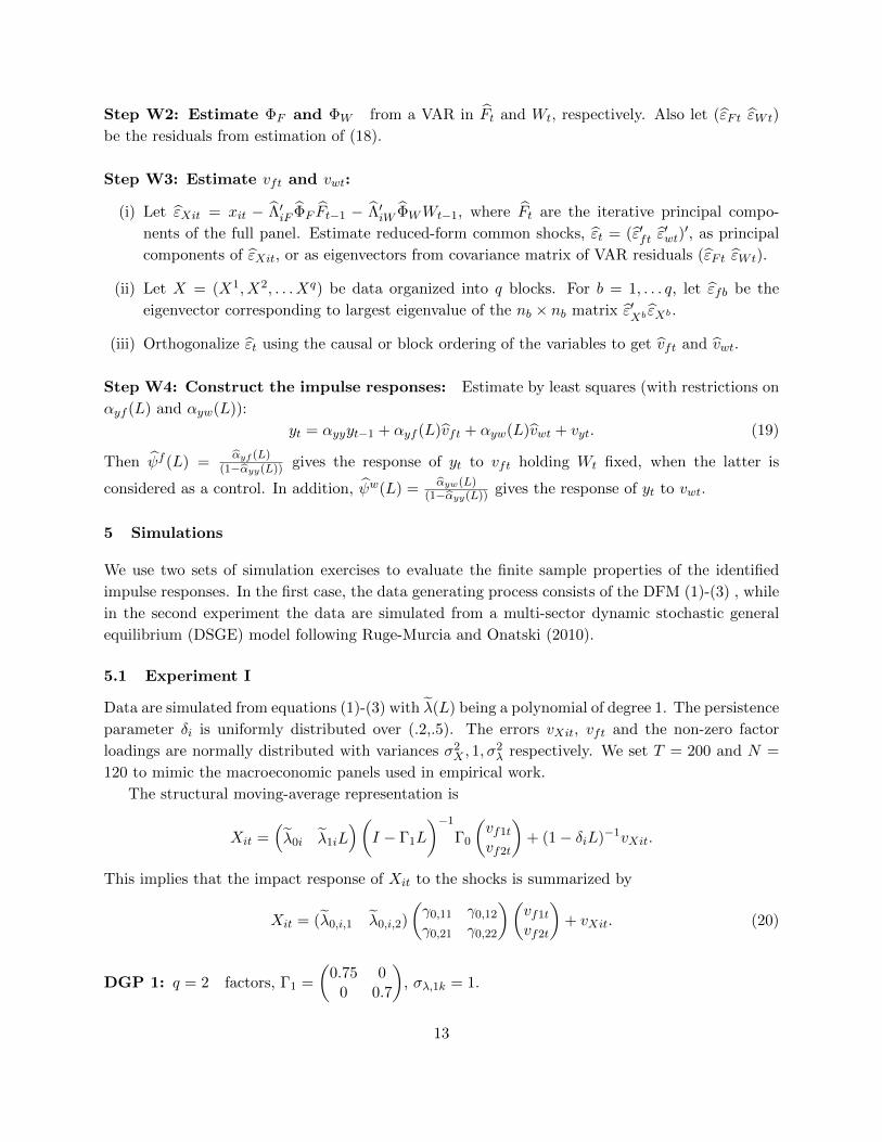
Step W2: Estimate ΦF and ΦW from a VAR in Ft and Wt, respectively. Also let (εFt εWt)
be the residuals from estimation of (18).
Step W3: Estimate vft and vwt:
(i) Let εXit = xit − Λ′iF ΦF Ft−1 − Λ′iW ΦWWt−1, where Ft are the iterative principal compo-
nents of the full panel. Estimate reduced-form common shocks, εt = (ε′ft ε′wt)′, as principal
components of εXit, or as eigenvectors from covariance matrix of VAR residuals (εFt εWt).
(ii) Let X = (X1, X2, . . . Xq) be data organized into q blocks. For b = 1, . . . q, let εfb be the
eigenvector corresponding to largest eigenvalue of the nb × nb matrix ε′Xb εXb .
(iii) Orthogonalize εt using the causal or block ordering of the variables to get vft and vwt.
Step W4: Construct the impulse responses: Estimate by least squares (with restrictions on
αyf (L) and αyw(L)):
yt = αyyyt−1 + αyf (L)vft + αyw(L)vwt + vyt. (19)
Then ψf (L) =αyf (L)
(1−αyy(L)) gives the response of yt to vft holding Wt fixed, when the latter is
considered as a control. In addition, ψw(L) =αyw(L)
(1−αyy(L)) gives the response of yt to vwt.
5 Simulations
We use two sets of simulation exercises to evaluate the finite sample properties of the identified
impulse responses. In the first case, the data generating process consists of the DFM (1)-(3) , while
in the second experiment the data are simulated from a multi-sector dynamic stochastic general
equilibrium (DSGE) model following Ruge-Murcia and Onatski (2010).
5.1 Experiment I
Data are simulated from equations (1)-(3) with λ(L) being a polynomial of degree 1. The persistence
parameter δi is uniformly distributed over (.2,.5). The errors vXit, vft and the non-zero factor
loadings are normally distributed with variances σ2X , 1, σ
2λ respectively. We set T = 200 and N =
120 to mimic the macroeconomic panels used in empirical work.
The structural moving-average representation is
Xit =(λ0i λ1iL
)(I − Γ1L
)−1
Γ0
(vf1t
vf2t
)+ (1− δiL)−1vXit.
This implies that the impact response of Xit to the shocks is summarized by
Xit = (λ0,i,1 λ0,i,2)
(γ0,11 γ0,12
γ0,21 γ0,22
)(vf1t
vf2t
)+ vXit. (20)
DGP 1: q = 2 factors, Γ1 =
(0.75 0
0 0.7
), σλ,1k = 1.
13

case a: Γ0 = I, case b: Γ0 =
(1 0
0.5 1
), σλ,2k = 0.8.
The N variables are ordered such that the first N/2 variables respond contemporaneously to
both shocks and are labeled ‘fast’. The last N/2 do not respond contemporaneously to shock 2 and
are labeled slow’. By design, X1t is a fast variable and XNt is a slow variable. This structure is
achieved by specifying
(λ0,i,1 λ0,i,2), i = 1, . . . , N/2 and (λ0,i,1 0) i = N/2 + 1, . . . , N.
Let Yt = (X1t, XN,t) be the two variables whose impulse responses are of interest. Since there are
no observed factors, estimation begins with E1 and E2. We consider both identification strategies
and estimate two FADL regressions, one for each variable in Yt. As a benchmark, we also estimate
the (infeasible) FADL regressions using the true common shocks, vft.
The results are summarized in Table 1. The top panel shows that for DGP 1a, the correlation
between vfjt and vfjt are well above 0.90 for both identification strategies. For DGP 1b, Method
(a) is more precise than (b) but the latter is still quite precise. The correlation between vfjt and
vfkt, i 6= k, are numerically small. The middle panel of Table 1 reports the RMSE of the estimated
impulse responses when the shocks are observed. Given that there are two shocks, there are two
impulse responses to consider for each of the two variables. We use vfj → Xk to denote the response
of Xk to shock j, where k = 1 is the fast variable, and k = N is the slow variable. The third panel
reports results when the common shocks have to be estimated. The ψ are practically identical to
the analytical ones given by (20). Furthermore, the impact response of slow variable to second
shock is not statistically different from zero (not reported).
DGP 2: q = 2 latent and m = 1 observed factors Let σλ,jk = 1, σλ,1k = 1, σλ,2k = 0.8, and
σλ,3k = 0.7 and Γ1 =
0.75 0 00 0.7 00 0 0.65
.
case a: Γ0 = I, case b: Γ0 =
1 0 00.4 1 00.3 0.2 1
.
The ordering of structural shocks is vft = (vslowft , vmpft , vfastft ). The goal is (partial) iden-
tification of the effects of vmpft . Again, the N variables are divided between fast and slow: slow
variables do not respond on impact to second and third shocks, and at least one variable does not
respond immediately only to the third shock, such that the causal ordering holds.
After the common shocks are estimated and identified according to Methods RO and BO, two
FADL regressions are estimated for the two components in Yt: one fast and one slow variable. The
results are summarized in Table 2. As we are interested in partial identification of the second shock,
we only report results on the approximation of vmpft , and impulse responses of two variables to this
shock. As in the previous exercise, FADL regressions with true shocks produce impulse response
coefficients practically identical to the analytical ones. The estimated second shock is very close to
the true one and ψ(L) very close to true impulse response coefficients.
14

5.2 Experiment II
The previous simulation exercise served to evaluate if the estimation of FADL representation is able
to recover the true shocks and generate accurate impulse responses when the DGP is a DFM. Now,
we replicate exactly the same simulation design from Ruge-Murcia and Onatski (2010): a large
multi-sector DSGE able to produce hundreds of aggregate and disaggregate series. The objective
is to use this laboratory to evaluate if the FADL methodology can recover the impulse responses
to an exogenous monetary policy shock and compare its performance to standard FAVAR analysis.
We proceed in following steps:
1. Simulate 156 series that consist of: 6 aggregate and 150 sectoral variables (output, hours
worked, wages, consumption and inflation). All the details are in Ruge-Murcia and Onatski
(2010) and Matlab codes are publicly available.
2. Estimate FADL and FAVAR models on simulated data and produce impulse responses to
exogenous money growth shock. Compare their performance in terms of mean (and median)
squared (and absolute) errors.
The previous steps are repeated 1000 times. The results for aggregate series are summarized
in Table 3. For the sake of space, additional results and estimation details are presented in the
not-for-publication online Appendix. Overall, FADL models provide better approximations of true
impulse responses of aggregate series, especially when the performance is measured by median
RMSE and by mean absolute error. Also, we remark that estimating common shocks from a subset
of 118 series, out of 156, often shrinks the estimation error.5 Moreover, the uncertainty around
median impulse response estimates is much smaller in case of FADL model. Similar results for
sectoral series are summarized in the online Appendix.
6 Two Examples
In this section, we use FADL to analyze two problems: measuring the dynamic effects of monetary
policy shocks and news (technology) shocks.
6.1 Example 1: Effects of a Monetary Policy Shock
As in Bernanke, Boivin, and Eliasz (2005), the monetary authority observes Nslow variables (such
as measures of real activity and prices) collected into Xslowt when setting the interest rate Rt but
does not observe Nfast variables (such as financial data) collected into Xfastt . In this exercise, Rt
is an observed factor. Let vft = (vslowft , vmpft , vfastft ) be the vector of q common shocks, where
vmpft is the monetary policy shock, vfastft is a vector q1 shocks, specific to Xfast, and vslowft is a vector
of q2 shocks, specific to Xslowt respectively, with q = q1 + q2 + 1. The issue of interest is (partial)
identification of the effects of monetary policy shock, meaning that the effects due to vslowft and
vfastft are not of interest.
5A set of sectoral series, that do not respond significantly enough to money growth shock, have been removedfrom Xt and form the dataset XOTH . See tables in the online Appendix.
15

Bernanke, Boivin, and Eliasz (2005) identify the monetary policy shock by assuming that Ψf0 is
a block lower triangular structure. This involves restrictions on Nslow > q2 variables. In a data rich
environment, some of these restrictions could well be invalid. Instead, we consider an alternative
identification strategy using fewer restrictions. It is based on Assumption RO which can be achieved
by choosing the first q variables to compose of q1 (slow) indicators of real activity and prices, followed
by the monetary policy instrument.6 The Assumption BO, which identifies the shocks at the block
level, is also easy to apply. The data are ordered as Yt = (Xslow′t , Rt, Xfast′
t )′. After estimating
vslowft from Xslowt and and vfastft from Xfast
t , the monetary policy shocks are the residuals from a
regression of Rt on current and lag values of vslowft . By construction, the estimated structural shocks
are mutually uncorrelated under both RO and BO assumptions. A FADL in all the shocks is then
estimated for each variable of interest.
In terms of matrix Ψf0 , Bernanke, Boivin, and Eliasz (2005) assumes:
Ψf0 =
ψ0,1,1
Nslow×q1
0Nslow×1
0Nslow×q2
ψ0,2,1
1×q1
ψ0,2,2
1×1
01×q2
ψ0,3,1
Nfast×q1
ψ0,3,2
Nfast×1
ψ0,3,3
Nfast×q2
.
Assumptions RO and BO both assume that the top q × q block of Ψf
0 is lower triangular:
Ψf0,1:q,1:q =
ψ0,1:q,1
q1×q1
0q1×1
0q1×q2
ψ0,2:q,1
1×q1
ψ0,2:q,2
1×1
01×q2
ψ0,3:q,1
q2×q1
ψ0,3:q,2
q2×1
ψ0,3:q,3
q2×q2
.
However, the Ψf
0 matrix and vft identified by RO will be different from those identified by BO.
Under Assumption RO, all N series are used to estimate the q vector εft. Thus any q series in the
training sample can be used to identify primitive shocks v. Under Assumption BO, εjft is estimated
from block j of Xt. Thus, the j shock in vft is identified from one of the Nj series in block j
of Xt. Assumption BO also allows a priori economic restrictions to be imposed on some or all
variables within the blocks. For example, we can restrict all Nslow series not to react on impact to
a monetary policy shock, while the response of fast moving variables is unrestricted. Since these
restrictions are imposed on equation by equation basis, they do not affect the estimation nor the
identification of structural shocks.7
6One may also add q2 financial indicators at the end of the recursion, but Bernanke, Boivin, and Eliasz (2005)found that there is little informational content in the fast moving factors that is not already accounted for by thefederal funds rate.
7The restrictions can vary across series in the block. For example, one series could be restricted to respond only 2periods after the shock, the sign of another variables could be fixed, the shape of the impulse response function couldbe constrained for a third variables, and so on.
16
6.1.1 Data and Results
The training sample used to estimate the factors consists of 107 quarterly aggregate macroeconomic
and financial indicators over the extended sample 1959Q1- 2009 Q1. This data set consists of fast
and slow moving variables. The Federal funds rate (FFR) is treated as an observed factor. All data
are assumed stationary or transformed to be covariance stationary. The complete list of variables
is given in the online Appendix.
Our estimation differs from Bernanke, Boivin, and Eliasz (2005) in two ways. First, we use
quarterly data. Second, we estimate the factors by IPC to take care of autocorrelation in residuals.
According to information criteria in Amengual and Watson (2007) and Bai and Ng (2007), there
are q = 3 latent dynamic factors in the training sample. Identification is achieved by imposing a
causal ordering. We order commodity price inflation first, followed by GDP deflator inflation, un-
employment rate, and then FFR. Hence monetary policy is the last variable in this causal ordering,
which implies zero contemporaneous response to monetary policy by the slow moving variables.
We only impose restrictions on q series (one from each block) while Bernanke, Boivin, and Eliasz
(2005) impose restrictions on all series belonging to the slow moving block.
Compared to Stock and Watson (2005), we impose the same minimal number of restrictions to
identify the structural shocks, but our approach differs in estimating the impulse response functions.
Instead of constructing impulse response coefficients of Xt as (I−D(L))Λ(I−Γ1(L))−1Γ0, we rather
estimate the product, ψfi (L), equation by equation for any element of Xt and XOTHt .
The 12 period impulse responses are presented in Figure 1. As in Bernanke, Boivin, and Eliasz
(2005), controlling for the presence of common shocks resolves anomalies found in the literature.
After a monetary policy shock, the fast moving variables such as Treasury bills increase immediately,
while stock prices, housing starts, and consumer expectations fall. Furthermore, many measures of
the slow variables including real activity and prices decline as a result of the shock without evidence
of a price puzzle. The exchange rate appreciates fully on impact, with no evidence of overshooting.
The results for the variables of interest are in line with Christiano, Eichenbaum, and Evans (2000)
who use recursive and non-recursive identification schemes to study the effects of monetary policy,
using small VARs. However, once the common shocks are estimated, the effects of monetary policy
can be studied for many variables, not just the q variables used in identification. The scope of the
analysis is much larger than a small VAR.
To check the validity of the factor structure in series not in the training sample, we consider
XOTHt consisting of hundreds of disaggregated series. Amongst these are (i) sectoral CPI, PCE,
and PPI measures of inflation, (ii) disaggregated employment series, (iii) investment measures (iv)
18 consumption series, and (v) industrial production sectoral data. For each of these additional
variables, the Wald test is used to test the null hypothesis that all coefficients in αyf (L) are jointly
zero. The null hypothesis cannot be rejected at the five percent level for many series including one
sectoral CPI, 15 PCE, one employment, one investment and two consumption series. For these
series, the data does not support the presence of a factor structure.
We then proceed to analyze the effects of monetary policy on variables in XOTHt . Interestingly,
the impulse responses of variables not affected by vft display price-puzzle like features. As seen in
the top panel of Figure 2 for some of these variables, an increase in the Fed Funds rate increases
17

rather than lowers prices. The bottom panel displays results for four series with significant αyf (L).
For these latter set of variables, the impulse responses are similar to those reported for the variables
in the training sample, namely, that an increase in the Fed funds rate lowers prices.8
6.1.2 Asymmetric Effects of a Monetary Policy Shock
In order to show the flexibility of the FADL approach, we now verify the asymmetry of mone-
tary policy effects. In the standard VAR (and FAVAR) approach, one must specify and estimate
a nonlinear model to allow for asymmetric impulse responses.9. In FADL framework this is eas-
ily handled by adding positive and negative values of the identified monetary policy shock time
series separately to each univariate regression in equation (16). Let vMP+ft be a time series of
positive monetary policy shocks and zero elsewhere, and vMP−ft be a vector containing negative
shocks. We remove vMPft from FADL regression 16 and add [vMP+
ft vMP−ft ]. Then, impulse re-
sponses to both contractionary and expansionary monetary policy shocks are easily computed by
inverting the autoregressive part. Another approach is adopted by Angrist, Jorda, and Kuersteiner
(2013) and Barnichon and Matthes (2014) who approximate the impulse responses directly from
the MA representation using Gaussian basis functions and with a semi-parametric estimator based
on propensity score weighting respectively. Our framework is computationally much easier, is not
subject to non-fundamentalness problem and allows to study the asymmetry of monetary policy
effects on hundreds of economic and financial indicators.
The results are presented in Figures 3 to 6. We find that contractionary monetary policy
causes more significant effects on several measures of economic activity. First, Figure 3 shows
the impulse responses of GDP, Industrial production (IP), Employment and Consumption after
contractionary and expansionary monetary policy shocks. It reveals that the response of these real
activity variables are much less significant after the expansionary shock compared to their responses
to a contractionary policy, suggesting that only (unexpected) tightening in monetary policy have
important (statistical and economical) impacts. The IRFs of all 24 series are presented in online
Appendix. Second, the comparison of point estimates in Figure 4 shows that, in general, the
asymmetric contractionary shock produces more pronounced effects on real activity, consumption,
credit and housing starts than in the case of the average impulse. Third, expansionary shock
generates lot of movements in these series compared to the symmetric responses, see Figure 5,
except for the consumer expectations that reacts much more. Fourth, we find quite symmetric
effects of the monetary policy on financial markets, as measured by the IRFs of Treasury Bills
and SP500 returns. Finally, Figure 6 shows the variance decomposition after the asymmetric
contractionary and expansionary monetary policy shocks. Interestingly, the expansionary shock is
much more important for interest rate, M2 and consumer expectations, while the contractionary
shock dominates for real activity series.
8The impulse responses of all sectoral variables from XOTHt are presented in the online Appendix. The responses
of many disaggregated series are in line with theory: a decline of real activity and price indicators across severalsectors after an adverse monetary policy shock. In case of employment variables, only mining and government sectorseries diverge from others during the first year after the shock, while the price indicators of some nondurable goodssectors present the price puzzle behavior.
9See Cover (1992) and Weise (1999) among others.
18

6.2 Example 2: Effects of a News Shock
Beaudry and Portier (2006) consider technology and news shocks, vft = (vTFPt vNSt )′, interpreted
as an announcement of future change in productivity. They are interested in the effects of these
two shocks on productivity X1t. Consider identification by the short run restrictions. Suppose that
the first N1 variables X1t ⊂ Xt do not respond immediately to vNSt , but its response to vTFPt is
unrestricted. Then Ψf0 is lower block triangular, viz:
Ψf0 =
ψf0,1,1 0...
...
ψf0,N1+1,1 ψf0,N1+1,2...
...
ψf0,N,1 ψf0,N,2
≡
Ψf0,1:N1,1
01:N1,1
. . . . . .
Ψf0,N1+1:N,1 Ψf
0,N1+1:N,2
.
This structure can be achieved if Λ0 and Γ0 are both lower block triangular, ie.
Λ0
N×2
=
λ0,1,1 0
......
λ0,N1+1,1 λ0,N1+1,2...
...λ0,N,1 λ0,N,2
=
Λ0,1:N1,1... 0N1×1
Λ0,N1+1:N,1... Λ0,N1+1:N,2
and Γ0
2×2
=
(Γ0,11 0Γ0,21 Γ0,22.
)
The zero restriction should hold for all series in the first block. But since there are only two
shocks, any two series permit exact identification provided one is from X1t , one from X2
t , and one
restriction is imposed on Ψf0 . Beaudry and Portier (2006) only uses two variables (X1t, XNt) for
analysis where X1t is a measure of TFP and XNt is stock price. We allow for N > 2 variables. But
unlike standard VARs which require restrictions of order N2 to identify N shocks, we use q series
to exactly identify q = 2 shocks. As discussed earlier, instead of putting restrictions on Γ0 or Λ0
separately, our restrictions are imposed on the relevant row(s) of Ψf0 = Γ0Λ0. The bivariate system
has the property that(X1t
XNt
)=
(ψf0,11 0
ψf0,21 ψf0,22
)(vTFPt
vNSt
)+∞∑j=1
(ψfj,11 ψfj,12
ψfj,21 ψfj,22
)(vTFPt−jvNSt−j
).
The number of identifying restrictions used in the FADL is of order q2 irrespective of N . This also
contrasts with standard FAVARs which impose many overidentifying restrictions. In our setup, a
large N is desirable for FADL because it improves estimation of vft. Long run restrictions can
similarly be imposed so that Ψf (1) is block lower triangular. A FADL leads to exact identification
using the salient features of the factor model.
6.2.1 Data and Results
Our data consists of Xt = (XTFPt , XSP
t , XOTHt ), where XTFP
t contains six TFP measures from
FRB San Francisco, XSPt is a vector of eight S&P and Dow Jones aggregate stock price indicators,
19
and XOTHt is a vector of 104 macroeconomic time series used in the previous example but with the
stock prices removed.10 Beaudry and Portier (2006) only use one series of the six series in XTFPt
and one series in XSPt at the time. Forni, Gambetti, and Sala (2011) use the same TFP series and
some of our stock price measures.
Two identification strategies are considered:
i (Recursive Ordering) estimate two common shocks from Xt = (XTFPt , XSP
t ). Two series, one
from XTFPt and one from XSP
t are selected. By ordering the TFP series first, the rotation
matrix B that identifies the technology and the news shock is easily computed.
ii (Block Ordering) εTFPt is estimated exclusively from XTFPt and εSPt is estimated from XSP
t .
The identification is based on the structure(εTFPt
εSPt
)=
(a11 0a21 a22
)(vTFPt
vNSt
).
Effectively, vTFPt = εTFPt and vNSt are the residuals from a projection of εSPt onto vTFPt . Note
that under both identification strategies the estimated shocks are mutually uncorrelated.
Once vTFPt and vNSt are available, variable by variable FADL equations are estimated for all
series in Xt. The zero impact restrictions are imposed for all TFP measures, while all other FADL
regressions are left unrestricted. The results for the two identification strategies and for news shocks
vNSt are given in Figures 7 and 8. We report results for stationary (transformed) data.11 The Table
5 contains p-values for Wald test for the null hypothesis of no factor structure in XTFPt , XSP
t and
XOTHt variables. The abbreviations ‘RO’, ‘BO’ stand for Assumption RO and BO respectively.
The null hypothesis is strongly rejected for many series.
Of special interest here are the responses to a positive news shock. The forward looking variables
such as stock prices, housing starts, new orders and consumer expectations increase on impact.
Consumption reacts positively. The wealth effect does not seem important enough such that the
worked hours also increase on impact.
Our results are in line with Beaudry and Portier (2006) for the pro-cyclical response of worked
hours. However, Barsky and Sims (2011) also estimate positive response of consumption and find
an immediate decrease of hours. Forni, Gambetti, and Sala (2011) find that both consumption and
hours respond negatively on impact. These differences can be due to the choice of variables used
to identify the shocks and to the variables selected for analysis. In particular, these studies used a
small set of worked hours measures. We check the sensitivity of our results to a much broader set
of available indicators.
To this end, we assess the sensitivity of our results (under the assumption of a block structure)
to additional variables as follows:
10The complete list of additional variables used in news shock application is available in online Appendix.11For the sake of space, the impulse responses to a positive technology shock vTFP
t are reported in the onlineAppendix. The estimated dynamic effects of technology shocks are in line with Christiano, Eichenbaum, and Vigfusson(2003) who suggest that technology improvements are pro-cyclical for real activity and hours measure, but contraryto Basu, Fernald, and Kimball (2006) and Gali (1999).
20

a Estimate εOTHt from the macro data XOTHt . Identification is now based onεTFPt
εSPtεOTHt
=
a11 0 0a21 a22 0a31 a32 a33
vTFPt
vNStvOTHt
.
b change the ordering to εTFPt , εOTHt with εSPt ordered last in view of the forward looking
nature of stock prices.
These results are denoted Block 2 and Block 3 respectively and correspond to BO2 and BO3 in
Tables and Figures. In a VAR setup, there would be 104 VARs to consider when there are 104
macro variables that might not be econometrically exogenous to TFP and stock prices. In the
factor setup, we only need to estimate one set of macro shocks from 104 macro series. As shown in
Figure 8, the effects of news shocks are smaller when the macro shocks are present. In other words,
omitted variables from the VAR could have biased the estimated effects of news shocks. However,
for an assumed q, the identified impulse responses are robust to the ordering of the variables.
As is well known, VARs involving hours worked are sensitive to whether the hours series is
in level or in difference, see for example, Feve and Guay (2009). We use the most conservative
specification Block 3 to further understand the dynamic response the level and growth of average
weekly hours (AWH) to a positive news shock. The results are presented in Figure 9. The dy-
namic responses of AWH and total hours indices are plotted in Figure 10. Regardless of the data
transformation, the hours series are pro-cyclical after the news shock. This exercise illustrates the
FADL can be used to check the robustness of the results to many other measures without affecting
the identification of structural shocks.
7 Conclusion
In this paper, we have proposed a new approach to analyze the dynamic effect of common shocks
in a data-rich environment. After estimating the common shocks from a large panel of data and
imposing a minimal set of identification restrictions, the impulse responses are obtained from an
autoregression in each variable of interest, augmented with a distributed lag of structural shocks.
The FADL framework presents several advantages. The method is more robust to a fully
structural factor model when the identifying factor restrictions do not hold universally. Since the
impulse responses are obtained from a set of regressions, the restrictions are easy to impose, and
implications of the factor model can be tested. The estimation of common shocks is less likely to be
affected by the presence of weak factors. The FADL methodology is used to measure the effects of
monetary policy shocks, and to news and technology shocks. The approach allows us to go beyond
existing structural FAVAR, and to validate restrictions of the factor model.
21

Appendix A: Consistency of Dynamic Multipliers Least Squares Estimates
Start from the infeasible regression (6) and use vft = Γ−10 εft, εft = J−1
NT εft to get
yt = α∗yy(L)yt−1 + α∗yf (L)Γ−10 εft + α∗yf (L)Γ−1
0 J−1NT εft − α
∗yf (L)Γ−1
0 J−1NT εft + v∗yt
= α∗yy(L)yt−1 + αyf (L)εft + vyt,
where αyf (L) = α∗yf (L)Γ−10 J−1
NT and vyt = v∗yt − αyf (L)(εft − JNT εft). Without loss of generality,
assume py = 1 and pf = 0 and write the model in matrix form
y = zδ + e, (21)
where z = (zyt, εft) = (yt−1, εft), and δ = [α∗yy(1), αyf (0)]′. Let z = (yt−1, JNT εft) so that
δ∗ = [α∗yy(1), α∗yf (0)Γ−10 J−1
NT ]′ are the parameters from infeasible FADL regression when εft are
observed. Let Szz = T−1∑T
t=1 ztz′t. Least squares estimation of (21) yields
√T (δ − δ) = S−1
zz T−1/2z′e
= S−1zz T
−1/2z′e+ S−1zz T
−1/2z′(εfJ′NT − εf )αyf (0)′.
Following Bai and Ng (2006), 1T
∑Tt=1(εft − JNT εft)z′t = Op(C
−2NT ), and thus
T−1/2z′(εf − εfJ ′NT ) = Op(T1/2C−2
NT )→ 0 if√T/N → 0.
In addition,
T−1/2z′e = T−1/2(z′ye JNT ε′fe) + op(1)
= T−1/2MNT z′e+ op(1),
where MNT = diag(I, JNT ) and z′ = (z′y ε′f ). Under standard assumptions, T−1/2z′e→ N(0,Σze),
where Σze = plimSze = T−1∑T
t=1 ztz′te
2t . Thus,
√T (δ − δ) = S−1
zz MNTT−1/2z′e+ op(1)→ N(0,Σ
δ),
where Σδ
= plimS−1zz MNTΣzeM
′NTS
−1′zz . In addition,
Szz = MNTSzzM′NT + op(1)→MΣzzM
′.
Thus, the asymptotic covariance matrix of δ reduces to
Σδ
= M−1′Σ−1zz ΣzeΣ
−1zzM
−1
which can be estimated by Σδ
= S−1zz ΣzeS
−1zz . If
√T/N → c > 0, then T−1/2z′(εf − εfJ ′NT ) does
not vanish and δ will have an asymptotic bias, see Ludvigson and Ng (2009) for details.
We have shown that the least squares estimates of αyf (L) will consistently estimate α∗yf (L)Γ−10 J−1
NT .
Hence, to get consistent estimates of the orthogonalized impulse responses we need to impose a
priori restrictions in terms of B = Γ−10 J−1
NT .
22
Appendix B: Relation to Other Methods with Observable Factors
The estimated common shocks are treated as regressors of a FADL. As such, a priori restrictions on
the impulse response functions can be directly imposed in estimation of the FADL by least squares.
The approach is simpler and more transparent than existing implementations of structural FAVARs.
Consider the identification of monetary policy shocks in the presence of other shocks as in
Bernanke, Boivin, and Eliasz (2005). Their point of departure is a static factor model with latent
and observed factors:
Xt = ΛFFt + ΛRRt + ut (22)[FtRt
]= Φ
[Ft−1
Rt−1
]+ ηt (23)
where Ft is vector of r latent factors and Rt is the observed factor (usually Federal Funds Rate or
3-month Treasury Bill). The authors organize the N = 120 data vector Xt into a block of slow-
moving’ variables that are largely predetermined, and another consisting of ‘fast moving’ variables
that are sensitive to contemporaneous news. The idiosyncratic errors are assumed to be serially
uncorrelated.
BBE Identification
1 Estimate Ft.
i Let C(Ft, Rt) be the K principal components of Xt.
ii Let XSt be NS ‘slow’ moving variables that do not respond immediately to a monetary
policy shock. Let the K principal components of XSt be C?(Ft).
iii Define Ft = C(Ft, Rt) − bRRt where bR is obtained by least squares estimation of the
regression
C(Ft, Rt) = bCC?(Ft) + bRRt + et.
2 Estimate the loadings by regressing Xt on Ft and Rt: ΛF and ΛR.
3 Estimate the FAVAR given by (23) and let ηt be the residuals. From the triangular decom-
position of the covariance of ηt, let A0 be a lower triangular matrix with ones on the main
diagonal Then ηt = A0εt are the monetary policy shocks.
4 Obtain IRFs for Ft and Rt by inverting (23) and using A0
5 Multiplying the IRFs from the previous step by ΛF and ΛR to obtain the IRFs for Xt.
The novelty of the BBE analysis is that Step (1) accommodates the observed factor Rt when
Ft is being estimated. By construction, C(Ft, Rt) spans the space spanned by Ft and Rt while
C∗(Ft) spans the space of common variations in variables that do not respond contemporaneously
to monetary policy. Since Rt is observed, the regression then constructs the component of Ct that
is orthogonal to Rt. Once Ft is available, Step (2) is straightforward. Under the BBE scheme, the
23

common shocks are identified in Step (3) when a FAVAR in (Ft, Rt) is estimated. Because Ft may
be correlated contemporaneously with Rt, the monetary policy shocks are identified by ordering Rtafter Ft in (23).12
The lower triangular of A0 is not enough to identify the structural shocks as the response
depends on the product(ΛF ΛR
)A0.13 Thus, BBE impose additional restrictions. In particular,
the K slow moving variables are ordered first in Xt. Furthermore, the K × K block of ΛF is
identity, and the first element in ΛR is zero. As a result, the first K+ 1×K+ 1 part of the product(ΛF ΛR
)A0 is lower triangular. For K = 2, 1 0 0
0 1 0λ31 λ32 λ33
1 0 0a21 1 0a31 a32 1
The structural model is just-identified.
Stock and Watson (2005) The SW approach treats monetary policy as a dynamic factor.
The identification assumptions are that (i) the monetary policy shock does not affect the slow-
moving variables contemporaneously; and (ii) the slow-moving shock and monetary policy affects
the Fed Funds rate contemporaneously. Thus, as in Bernanke, Boivin, and Eliasz (2005), the
slow-moving variables are ordered first, followed by the Fed funds rate, and then the fast-moving
variables. The point of departure is that εXt = Λεft + vXt is assumed to have a factor structure
and εft = Gηt = GBvft. Letting C = GB, the errors are related by
εXt = ΛCvft + vXt
where vft is of dimension q. The steps are as follows:
1 Let εXt into (εslowX,t , εfedX,t and εfastX,t ) corresponding to the three types of variables.
2 Let uFt, the residuals from a VAR in the static factors constructed from the full panel, X.
3 Let the factor component of εfedX,t be the fit from a reduced rank regression of εslowX,t and uFt.
4 Take the monetary shocks to be the residuals from a projection of of εfedX,t onto vslowX,t .
If there are qslow and qfast factors in εslowXt and εfastXt respectively, then q = qslow + qfast + 1. The
identification scheme makes use of the fact that vslowX,t spans the space of εslowX,t and can thus be
12Boivin, Giannoni, and Stevanovic (2010) use an alternative way to estimate Ft that does not rely on organizingthe variables into fast and slow.
1 Initialize Ft to be the K first principal components of Xt.
2 (i) Regress Xt on Ft and Rt, to obtain ΛF,jt and ΛR,j
t . (ii) Compute Xjt = Xt − ΛR,0
t Rt (iii) Update Ft as the
first K principal components of Xt
By construction, Ft is contemporaneously uncorrelated with Rt This is possible because the step that estimates thelatent factors controlling for the presence of the observed factors is separated from identification of structural shock.In BBE, ηt depends on the choice of variables used in the first stage to estimate Ft.
13In BBE application, Step 2 estimates of the loadings of slow moving variables to Rt are close to zero.
24

identified from a projection of εslowX,t on uFt. An additional step is needed to estimate the common
variations between uFt and εslowX,t . This procedure sequentially estimates the rotation matrix B14.
Note that the identification restrictions are imposed directly on the impact coefficients matrix of
the structural moving average representation of Xt, and the structural model is overidentified. The
method is not easily generalizable to other models in which the shocks do not have a block recursive
structure implicit in the model.
FGLR: Forni, Giannone, Lippi, and Reichlin (2009) provides a framework for structural FAVAR
analysis. The method is applied to identify monetary policy shocks in Forni and Gambetti (2010).
1 let Λ be a N × r matrix of estimated loadings and Ft be the static principal components.
Estimate a VAR in Ft to get Γ(L) and the residuals uFt.
2 Perform a spectral decomposition of the covariance matrix of uFt. Let M be a diagonal matrix
consisting of the largest eigenvalue of uF u′F and let K be the r × q matrix of eigenvectors.
3 Let S = KM . The non-orthogonalized impulse responses are given by
Ψη(L) = Λ(I − Γ(L))−1S.
Step (2) is a consequence of the fact that the VAR in Ft is singular. Step (3) rotates Ψη by a
q × q matrix of restrictions. Unlike the partial identification analysis of Stock and Watson (2005),
this method estimates the impulse responses for the system as a whole. Mis-specification in a
sub-system can affect the entire analysis, but the estimates are more efficient if every aspect of the
factor model is correctly specified.
14Boivin, Giannoni, and Stevanovic (2013) find that the rotation of principal components by B gives interpretablefactors.
25

Table 1: Simulation Experiment I, DGP 1
corr(vft, vft)
a. Recursive Ordering b. Block Ordering
DGP 1a
(0.9844 0.03080.0636 0.9790
) (0.9825 0.05620.0953 0.9030
)DGP 1b
(0.9843 0.03130.0638 0.9777
) (0.9805 0.08740.1188 0.8706
)RMSE of Impulse Responses: vft observed
vf1 → X1 vf2 → X1 vf1 → XN vf2 → XN
DGP 1a 0.0415 0.0412 0.0426 0.0414DGP 1b 0.0409 0.0394 0.0422 0.0425
RMSE of Impulse Responses Using vfta. Recursive Ordering b. Block Ordering
vf1 → X1 vf2 → X1 vf1 → XN vf2 → XN vf1 → X1 vf2 → X1 vf1 → XN vf2 → XN
DGP 1a 0.2452 0.2228 0.2299 0.1963 0.2558 0.2642 0.2366 0.2032DGP 1b 0.2994 0.2453 0.2702 0.1953 0.2954 0.3556 0.2556 0.2578
This Table presents a summary of results from the simulation experiment I, DGP 1. It shows the correlation between
the true and the estimated common shocks, the Root Mean Squared Error (RMSE) of impulse responses from the
infeasible FADL regression when vft is observed, and the RMSE from the feasible FADL regression when vft is used
instead. X1 is the ‘fast’ moving series that responds on impact to both shocks, while XN the ‘slow’ variable that does
not respond on impact to vf2.
Table 2: Simulation Experiment I, DGP 2
corr(vmpft , vmpft )
a. Recursive Ordering b. Block OrderingDGP 2a 0.9747 0.9629DGP 2b 0.9774 0.9620
RMSE of Impulse Responses: vf Observed
vf2 → X1 vf2 → XN
DGP 2a 0.0406 0.0417DGP 2b 0.0399 0.0419
RMSE of Impulse Responses: vf Estimated
a. Recursive Ordering b. Block Orderingvf2 → X1 vf2 → XN vf2 → X1 vf2 → XN
DGP 2a 0.2743 0.2285 0.2760 0.1996DGP 2b 0.3155 0.2781 0.3391 0.2466
This Table presents a summary of results from the simulation experiment I, DGP 2. It shows the results only with
respect to the shock of interest: vmpft .
26
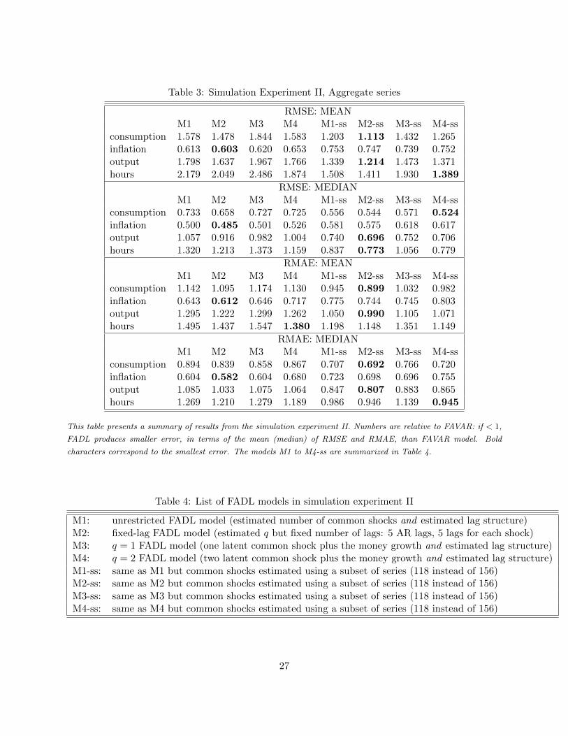
Table 3: Simulation Experiment II, Aggregate series
RMSE: MEANM1 M2 M3 M4 M1-ss M2-ss M3-ss M4-ss
consumption 1.578 1.478 1.844 1.583 1.203 1.113 1.432 1.265inflation 0.613 0.603 0.620 0.653 0.753 0.747 0.739 0.752output 1.798 1.637 1.967 1.766 1.339 1.214 1.473 1.371hours 2.179 2.049 2.486 1.874 1.508 1.411 1.930 1.389
RMSE: MEDIANM1 M2 M3 M4 M1-ss M2-ss M3-ss M4-ss
consumption 0.733 0.658 0.727 0.725 0.556 0.544 0.571 0.524inflation 0.500 0.485 0.501 0.526 0.581 0.575 0.618 0.617output 1.057 0.916 0.982 1.004 0.740 0.696 0.752 0.706hours 1.320 1.213 1.373 1.159 0.837 0.773 1.056 0.779
RMAE: MEANM1 M2 M3 M4 M1-ss M2-ss M3-ss M4-ss
consumption 1.142 1.095 1.174 1.130 0.945 0.899 1.032 0.982inflation 0.643 0.612 0.646 0.717 0.775 0.744 0.745 0.803output 1.295 1.222 1.299 1.262 1.050 0.990 1.105 1.071hours 1.495 1.437 1.547 1.380 1.198 1.148 1.351 1.149
RMAE: MEDIANM1 M2 M3 M4 M1-ss M2-ss M3-ss M4-ss
consumption 0.894 0.839 0.858 0.867 0.707 0.692 0.766 0.720inflation 0.604 0.582 0.604 0.680 0.723 0.698 0.696 0.755output 1.085 1.033 1.075 1.064 0.847 0.807 0.883 0.865hours 1.269 1.210 1.279 1.189 0.986 0.946 1.139 0.945
This table presents a summary of results from the simulation experiment II. Numbers are relative to FAVAR: if < 1,
FADL produces smaller error, in terms of the mean (median) of RMSE and RMAE, than FAVAR model. Bold
characters correspond to the smallest error. The models M1 to M4-ss are summarized in Table 4.
Table 4: List of FADL models in simulation experiment II
M1: unrestricted FADL model (estimated number of common shocks and estimated lag structure)M2: fixed-lag FADL model (estimated q but fixed number of lags: 5 AR lags, 5 lags for each shock)M3: q = 1 FADL model (one latent common shock plus the money growth and estimated lag structure)M4: q = 2 FADL model (two latent common shock plus the money growth and estimated lag structure)M1-ss: same as M1 but common shocks estimated using a subset of series (118 instead of 156)M2-ss: same as M2 but common shocks estimated using a subset of series (118 instead of 156)M3-ss: same as M3 but common shocks estimated using a subset of series (118 instead of 156)M4-ss: same as M4 but common shocks estimated using a subset of series (118 instead of 156)
27

Table 5: News Shock, p-values from Wald test for H0 : αyf (L) = 0
Variables in (XTFPt , XSP
t ) RO BO BO2 BO3
TFP 0 0 0 0TFP-util 0 0 0 0TFP-I 0 0 0 0TFP-C 0 0 0 0TFP-I-util 0 0 0 0TFP-C-util 0 0 0 0S&P: composite 0 0 0 0S&P: industrial 0 0 0 0S&P: dividend 0 0 0 0S&P: price/earning 0 0 0 0DJ: industrial 0 0 0 0DJ: composite 0 0 0 0DJ: transportation 0 0 0 0DJ: utilities 0 0 0 0
Variables in XOTHt
GDP 0 0 0 0IP 0 0 0 0CONSUMPTION 0 0 0 0INVESTMENT 0 0 0 0HOURS 0 0 0 0HOURS: Overtime 0 0 0 0EMPLOYEES: NONFARM 0,0262 0,0399 0 0CLF: EMPLOYED 0 0 0 0HELP-WANTED ADV 0 0 0 0AVG HOURLY EARNINGS 0 0 0 0CAPACITY UTILIZATION 0 0 0 0CONSUMER EXPECTATIONS 0 0 0 0UR 0 0 0 0EMPLOYEES ROMPENSATION 0 0 0 0CONSUMPTION: NONDUR 0 0 0 0CONSUMPTION: DURAB 0 0 0 0CONSUMER CREDIT 0,2422 0,2772 0 0HOUSING STARTS 0,0062 0,0027 0 0NEW ORDERS 0 0 0 0INVENTORIES 0,0718 0,1742 0 0FFR 0,3513 0,2612 0 0COMMODITY PRICES 0,0299 0,1384 0 0CPI 0,3527 0,5556 0 0GDP DEFLATOR 0,0438 0,0729 0 0
RO and BO refer to identification by causal and block ordering, respectively. The two blocks of data are XTFPt and
XSPt . Data from the macro block XM
t are also used in BO2 and BO3. BO2 uses the ordering TFP, SP, Macro. BO3
orders the macro variables before the stock prices.
28
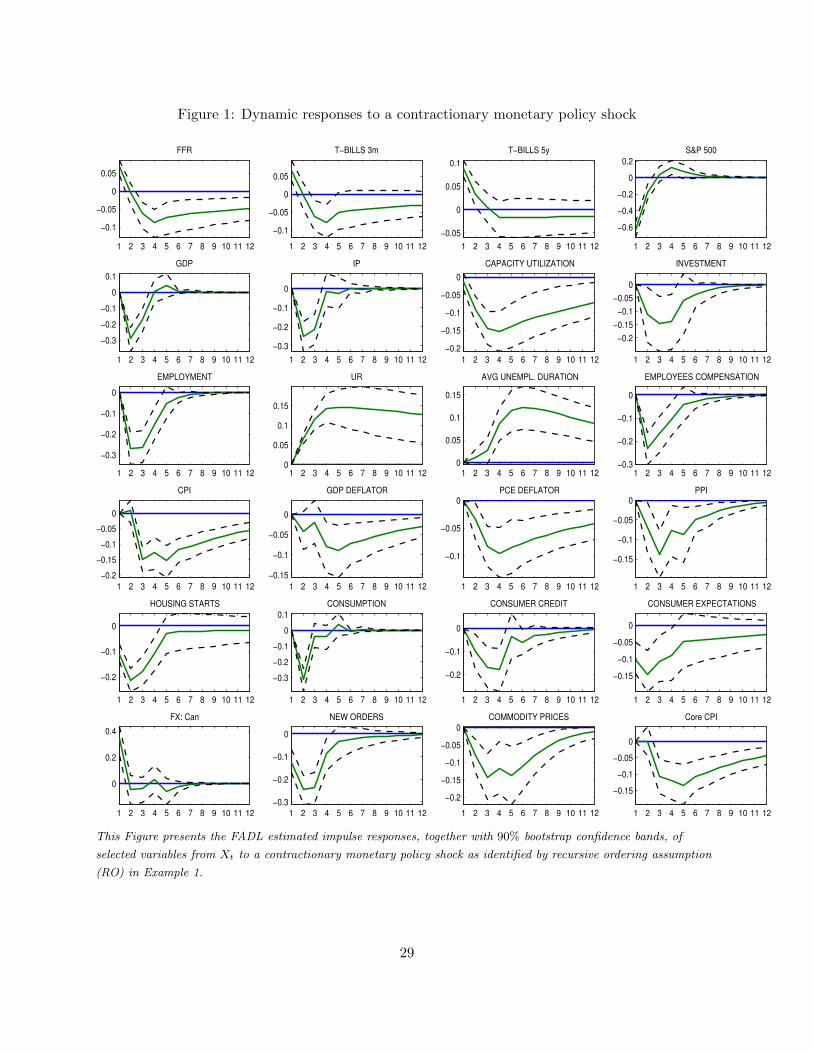
Figure 1: Dynamic responses to a contractionary monetary policy shock
1 2 3 4 5 6 7 8 9 10 11 12
−0.1
−0.05
0
0.05
FFR
1 2 3 4 5 6 7 8 9 10 11 12
−0.1
−0.05
0
0.05
T−BILLS 3m
1 2 3 4 5 6 7 8 9 10 11 12
−0.05
0
0.05
0.1
T−BILLS 5y
1 2 3 4 5 6 7 8 9 10 11 12
−0.6
−0.4
−0.2
0
0.2
S&P 500
1 2 3 4 5 6 7 8 9 10 11 12
−0.3
−0.2
−0.1
0
0.1
GDP
1 2 3 4 5 6 7 8 9 10 11 12
−0.3
−0.2
−0.1
0
IP
1 2 3 4 5 6 7 8 9 10 11 12
−0.2
−0.15
−0.1
−0.05
0
CAPACITY UTILIZATION
1 2 3 4 5 6 7 8 9 10 11 12
−0.2
−0.15
−0.1
−0.05
0
INVESTMENT
1 2 3 4 5 6 7 8 9 10 11 12
−0.3
−0.2
−0.1
0
EMPLOYMENT
1 2 3 4 5 6 7 8 9 10 11 120
0.05
0.1
0.15
UR
1 2 3 4 5 6 7 8 9 10 11 120
0.05
0.1
0.15
AVG UNEMPL. DURATION
1 2 3 4 5 6 7 8 9 10 11 12−0.3
−0.2
−0.1
0
EMPLOYEES COMPENSATION
1 2 3 4 5 6 7 8 9 10 11 12
−0.2
−0.15
−0.1
−0.05
0
CPI
1 2 3 4 5 6 7 8 9 10 11 12
−0.15
−0.1
−0.05
0
GDP DEFLATOR
1 2 3 4 5 6 7 8 9 10 11 12
−0.1
−0.05
0PCE DEFLATOR
1 2 3 4 5 6 7 8 9 10 11 12
−0.15
−0.1
−0.05
0PPI
1 2 3 4 5 6 7 8 9 10 11 12
−0.2
−0.1
0
HOUSING STARTS
1 2 3 4 5 6 7 8 9 10 11 12
−0.3
−0.2
−0.1
0
0.1
CONSUMPTION
1 2 3 4 5 6 7 8 9 10 11 12
−0.2
−0.1
0
CONSUMER CREDIT
1 2 3 4 5 6 7 8 9 10 11 12
−0.15
−0.1
−0.05
0
CONSUMER EXPECTATIONS
1 2 3 4 5 6 7 8 9 10 11 12
0
0.2
0.4
FX: Can
1 2 3 4 5 6 7 8 9 10 11 12
−0.3
−0.2
−0.1
0
NEW ORDERS
1 2 3 4 5 6 7 8 9 10 11 12
−0.2
−0.15
−0.1
−0.05
0COMMODITY PRICES
1 2 3 4 5 6 7 8 9 10 11 12
−0.15
−0.1
−0.05
0
Core CPI
This Figure presents the FADL estimated impulse responses, together with 90% bootstrap confidence bands, of
selected variables from Xt to a contractionary monetary policy shock as identified by recursive ordering assumption
(RO) in Example 1.
29
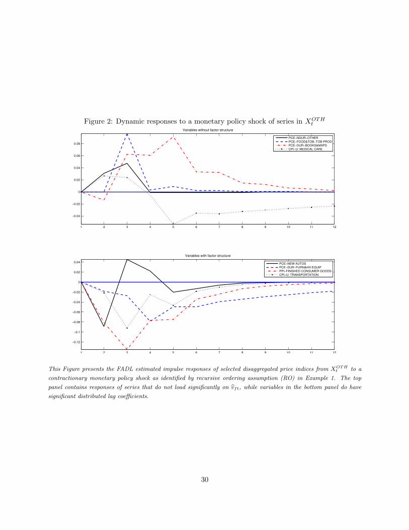
Figure 2: Dynamic responses to a monetary policy shock of series in XOTHt
1 2 3 4 5 6 7 8 9 10 11 12
−0.04
−0.02
0
0.02
0.04
0.06
0.08
Variables without factor structure
PCE−NDUR−OTHER
PCE−FOOD&TOB−TOB PROD
PCE−DUR−BOOKS&MAPS
CPI−U: MEDICAL CARE
1 2 3 4 5 6 7 8 9 10 11 12
−0.12
−0.1
−0.08
−0.06
−0.04
−0.02
0
0.02
0.04
Variables with factor structure
PCE−NEW AUTOS
PCE−DUR−FURN&HH EQUIP
PPI−FINISHED CONSUMER GOODS
CPI−U: TRANSPORTATION
This Figure presents the FADL estimated impulse responses of selected disaggregated price indices from XOTHt to a
contractionary monetary policy shock as identified by recursive ordering assumption (RO) in Example 1. The top
panel contains responses of series that do not load significantly on vft, while variables in the bottom panel do have
significant distributed lag coefficients.
30

Figure 3: Asymmetric IRFs to contractionary and expansionary monetary policy shocks
1 2 3 4 5 6 7 8 9 10 11 12
−0.4
−0.3
−0.2
−0.1
0
0.1
0.2
GDP
Con
tract
iona
ry s
hock
1 2 3 4 5 6 7 8 9 10 11 12
−0.4
−0.3
−0.2
−0.1
0
0.1
0.2
IP
1 2 3 4 5 6 7 8 9 10 11 12
−0.5
−0.4
−0.3
−0.2
−0.1
0
EMPLOYMENT
1 2 3 4 5 6 7 8 9 10 11 12
−0.5
−0.4
−0.3
−0.2
−0.1
0
0.1
0.2
CONSUMPTION
1 2 3 4 5 6 7 8 9 10 11 12
−0.2
−0.1
0
0.1
0.2
0.3
GDP
Expa
nsio
nary
sho
ck
1 2 3 4 5 6 7 8 9 10 11 12
−0.1
−0.05
0
0.05
0.1
0.15
0.2
0.25
0.3
IP
1 2 3 4 5 6 7 8 9 10 11 12−0.15
−0.1
−0.05
0
0.05
0.1
0.15
0.2
0.25
0.3
EMPLOYMENT
1 2 3 4 5 6 7 8 9 10 11 12
−0.15
−0.1
−0.05
0
0.05
0.1
0.15
0.2
0.25
CONSUMPTION
This Figure presents the FADL estimated asymmetric impulse responses, together with 90% bootstrap confidence bands,
of selected variables from Xt to contractionary and expansionary monetary policy shocks as identified by recursive
ordering assumption (RO) in Example 1. The top 4 graphs show IRFs to a contractionary shock while the bottom
graphs present IRFs to an expansionary monetary policy shock.
31

Figure 4: Comparison of symmetric and asymmetric IRFs to a contractionary monetary policyshock
1 2 3 4 5 6 7 8 9 10 11 12
−0.05
0
0.05
FFR
Sym
Asym
1 2 3 4 5 6 7 8 9 10 11 12
−0.05
0
0.05
T−BILLS 3m
1 2 3 4 5 6 7 8 9 10 11 12
−0.02
0
0.02
0.04
0.06
0.08
T−BILLS 5y
1 2 3 4 5 6 7 8 9 10 11 12
−0.6
−0.4
−0.2
0
0.2
S&P 500
1 2 3 4 5 6 7 8 9 10 11 12
−0.3
−0.2
−0.1
0
0.1
GDP
1 2 3 4 5 6 7 8 9 10 11 12
−0.3
−0.2
−0.1
0
IP
1 2 3 4 5 6 7 8 9 10 11 12−0.2
−0.15
−0.1
−0.05
0CAPACITY UTILIZATION
1 2 3 4 5 6 7 8 9 10 11 12
−0.5
−0.4
−0.3
−0.2
−0.1
INVESTMENT
1 2 3 4 5 6 7 8 9 10 11 12
−0.4
−0.3
−0.2
−0.1
0EMPLOYMENT
1 2 3 4 5 6 7 8 9 10 11 120
0.05
0.1
UR
1 2 3 4 5 6 7 8 9 10 11 120
0.05
0.1
0.15
0.2
AVG UNEMPL. DURATION
1 2 3 4 5 6 7 8 9 10 11 12−0.4
−0.3
−0.2
−0.1
0
EMPLOYEES COMPENSATION
1 2 3 4 5 6 7 8 9 10 11 12
−0.15
−0.1
−0.05
0
CPI
1 2 3 4 5 6 7 8 9 10 11 12
−0.08
−0.06
−0.04
−0.02
0GDP DEFLATOR
1 2 3 4 5 6 7 8 9 10 11 12
−0.15
−0.1
−0.05
0PCE DEFLATOR
1 2 3 4 5 6 7 8 9 10 11 12
−0.2
−0.15
−0.1
−0.05
0PPI
1 2 3 4 5 6 7 8 9 10 11 12
−0.25
−0.2
−0.15
−0.1
−0.05
HOUSING STARTS
1 2 3 4 5 6 7 8 9 10 11 12
−0.4
−0.2
0
CONSUMPTION
1 2 3 4 5 6 7 8 9 10 11 12
−0.25
−0.2
−0.15
−0.1
−0.05
CONSUMER CREDIT
1 2 3 4 5 6 7 8 9 10 11 12
−0.15
−0.1
−0.05
0
0.05
CONSUMER EXPECTATIONS
1 2 3 4 5 6 7 8 9 10 11 12
0
0.2
0.4
FX: Can
1 2 3 4 5 6 7 8 9 10 11 12
−0.2
−0.1
0
NEW ORDERS
1 2 3 4 5 6 7 8 9 10 11 12
−0.15
−0.1
−0.05
0COMMODITY PRICES
1 2 3 4 5 6 7 8 9 10 11 12
−0.1
−0.05
0Core CPI
This Figure compares the FADL estimated symmetric (full line) and asymmetric (dotted line) impulse responses of
selected variables from Xt to a contractionary monetary policy shock as identified by recursive ordering assumption
(RO) in Example 1.
32

Figure 5: Comparison of symmetric and asymmetric IRFs to an expansionary monetary policyshock
1 2 3 4 5 6 7 8 9 10 11 12
−0.05
0
0.05
0.1
FFR
Sym
Asym
1 2 3 4 5 6 7 8 9 10 11 12
−0.05
0
0.05
0.1
T−BILLS 3m
1 2 3 4 5 6 7 8 9 10 11 12
−0.1
−0.05
0
T−BILLS 5y
1 2 3 4 5 6 7 8 9 10 11 12
0
0.2
0.4
0.6
S&P 500
1 2 3 4 5 6 7 8 9 10 11 12
−0.1
0
0.1
0.2
GDP
1 2 3 4 5 6 7 8 9 10 11 120
0.1
0.2
IP
1 2 3 4 5 6 7 8 9 10 11 120
0.05
0.1
0.15
CAPACITY UTILIZATION
1 2 3 4 5 6 7 8 9 10 11 12−0.2
−0.1
0
0.1
INVESTMENT
1 2 3 4 5 6 7 8 9 10 11 120
0.1
0.2
EMPLOYMENT
1 2 3 4 5 6 7 8 9 10 11 12
−0.2
−0.15
−0.1
−0.05
0UR
1 2 3 4 5 6 7 8 9 10 11 12
−0.1
−0.05
0
AVG UNEMPL. DURATION
1 2 3 4 5 6 7 8 9 10 11 12
0
0.1
0.2
EMPLOYEES COMPENSATION
1 2 3 4 5 6 7 8 9 10 11 12
0
0.05
0.1
0.15
0.2
CPI
1 2 3 4 5 6 7 8 9 10 11 12
0
0.05
0.1
0.15
GDP DEFLATOR
1 2 3 4 5 6 7 8 9 10 11 120
0.02
0.04
0.06
0.08
PCE DEFLATOR
1 2 3 4 5 6 7 8 9 10 11 120
0.05
0.1
PPI
1 2 3 4 5 6 7 8 9 10 11 12
0
0.05
0.1
0.15
0.2
HOUSING STARTS
1 2 3 4 5 6 7 8 9 10 11 12
0
0.1
0.2
0.3
CONSUMPTION
1 2 3 4 5 6 7 8 9 10 11 12
−0.05
0
0.05
0.1
0.15
CONSUMER CREDIT
1 2 3 4 5 6 7 8 9 10 11 120
0.05
0.1
0.15
0.2
CONSUMER EXPECTATIONS
1 2 3 4 5 6 7 8 9 10 11 12
−0.3
−0.2
−0.1
0
FX: Can
1 2 3 4 5 6 7 8 9 10 11 120
0.05
0.1
0.15
0.2
NEW ORDERS
1 2 3 4 5 6 7 8 9 10 11 120
0.05
0.1
0.15
COMMODITY PRICES
1 2 3 4 5 6 7 8 9 10 11 12
0
0.05
0.1
0.15
0.2
Core CPI
This Figure compares the FADL estimated symmetric (full line) and asymmetric (dotted line) impulse responses of
selected variables from Xt to an expansionary monetary policy shock as identified by recursive ordering assumption
(RO) in Example 1.
33

Figure 6: Variance decomposition after asymmetric expansionary and contractionary monetarypolicy shocks
0
0.05
0.1
0.15
0.2
0.25
0.3
0.35
% o
f va
ria
nce
exp
lain
ed
IPCPI
T−BILLS
3m M
2
CONSUMER C
REDIT
FX: C
an
CAPACIT
Y U
TILIZA
TION
CONSUMPTI
ON
EMPLO
YMENT
AVG H
OURLY
EARNIN
GS
HOUSIN
G S
TARTS
S&P 500
CONSUMER E
XPECTA
TIONS
GDP
Cor
e CPI
INVESTM
ENT
ASYM EXPANSIONARY.
ASYM CONTRACTIONARY
This Figure plots the FADL estimate of the variance decomposition of selected variables from Xt after expansionary
(blue line) and contractionary (black line) asymmetric monetary policy shocks as identified by recursive ordering
assumption (RO) in Example 1.
34

Figure 7: Dynamic responses of XTFPt and XSP
t to a positive news shock
1 2 3 4 5 6 7 8 9 10 11 120
0.05
0.1
0.15
0.2tfp
1 2 3 4 5 6 7 8 9 10 11 12−0.1
−0.08
−0.06
−0.04
−0.02
0
0.02tfp−util
1 2 3 4 5 6 7 8 9 10 11 120
0.05
0.1
0.15
0.2tfp−I
1 2 3 4 5 6 7 8 9 10 11 120
0.05
0.1
0.15
0.2tfp−C
1 2 3 4 5 6 7 8 9 10 11 12−0.2
−0.15
−0.1
−0.05
0tfp−I−util
1 2 3 4 5 6 7 8 9 10 11 12−0.1
−0.05
0
0.05
0.1tfp−C−util
1 2 3 4 5 6 7 8 9 10 11 120
0.2
0.4
0.6
0.8
1S&P: composite
1 2 3 4 5 6 7 8 9 10 11 120
0.2
0.4
0.6
0.8
1S&P: industrial
1 2 3 4 5 6 7 8 9 10 11 12−0.25
−0.2
−0.15
−0.1
−0.05
0S&P: dividend
1 2 3 4 5 6 7 8 9 10 11 120
0.05
0.1
0.15
0.2
0.25S&P: price/earning
1 2 3 4 5 6 7 8 9 10 11 12−0.5
0
0.5
1DJ: industrial
1 2 3 4 5 6 7 8 9 10 11 12−0.5
0
0.5
1DJ: composite
1 2 3 4 5 6 7 8 9 10 11 12−0.5
0
0.5
1DJ: transportation
1 2 3 4 5 6 7 8 9 10 11 12−0.2
0
0.2
0.4
0.6
0.8DJ: utilities
RO BO BO2 BO3
This Figure presents the FADL estimated impulse responses of all variables in XTFPt and XSP
t to a positive news shock
as identified by recursive ordering assumption (RO) and block ordering assumptions (BO, BO2, BO3) in Example 2.
35

Figure 8: Dynamic responses of selected series in XOTHt to a positive news shock
1 2 3 4 5 6 7 8 9 1011120
0.1
0.2
0.3
0.4
GDP
1 2 3 4 5 6 7 8 9 101112−0.2
0
0.2
0.4
0.6
IP
1 2 3 4 5 6 7 8 9 1011120
0.1
0.2
0.3
0.4
CONSUMPTION
1 2 3 4 5 6 7 8 9 101112−0.1
0
0.1
0.2
0.3
0.4
INVESTMENT
1 2 3 4 5 6 7 8 9 1011120
0.1
0.2
0.3
0.4
HOURS
1 2 3 4 5 6 7 8 9 1011120
0.1
0.2
0.3
0.4
HOURS: Overtime
1 2 3 4 5 6 7 8 9 101112−0.1
0
0.1
0.2
0.3
EMPLOYEES: NONFARM
1 2 3 4 5 6 7 8 9 1011120
0.1
0.2
0.3
0.4
CLF: EMPLOYED
1 2 3 4 5 6 7 8 9 1011120
0.1
0.2
0.3
0.4
HELP−WANTED ADV
1 2 3 4 5 6 7 8 9 101112−0.2
−0.1
0
0.1
0.2
AVG HOURLY EARNINGS
1 2 3 4 5 6 7 8 9 101112−0.1
0
0.1
0.2
0.3
CAPACITY UTILIZATION
1 2 3 4 5 6 7 8 9 1011120
0.05
0.1
0.15
0.2
0.25
CONSUMER EXPECTATIONS
1 2 3 4 5 6 7 8 9 101112−0.3
−0.2
−0.1
0
0.1
UR
1 2 3 4 5 6 7 8 9 1011120
0.1
0.2
0.3
0.4
EMPLOYEES COMPENSATION
1 2 3 4 5 6 7 8 9 101112−0.1
0
0.1
0.2
0.3
CONSUMPTION: NONDUR
1 2 3 4 5 6 7 8 9 101112−0.1
0
0.1
0.2
0.3
CONSUMPTION: DURAB
1 2 3 4 5 6 7 8 9 101112−0.1
−0.05
0
0.05
0.1
CONSUMER CREDIT
1 2 3 4 5 6 7 8 9 1011120
0.05
0.1
0.15
0.2
0.25
HOUSING STARTS
1 2 3 4 5 6 7 8 9 1011120
0.1
0.2
0.3
0.4
0.5
NEW ORDERS
1 2 3 4 5 6 7 8 9 101112−0.1
0
0.1
0.2
0.3
INVENTORIES
1 2 3 4 5 6 7 8 9 101112−0.04
−0.02
0
0.02
0.04
0.06
FFR
1 2 3 4 5 6 7 8 9 101112−0.05
0
0.05
0.1
0.15
0.2
COMMODITY PRICES
1 2 3 4 5 6 7 8 9 101112−0.06
−0.04
−0.02
0
0.02
0.04
CPI
1 2 3 4 5 6 7 8 9 101112−0.1
−0.05
0
0.05
0.1
GDP DEFLATOR
RO BO BO2 BO3
This Figure presents the FADL estimated impulse responses of selected variables in XOTHt to a positive news shock
as identified by recursive ordering assumption (RO) and block ordering assumptions (BO, BO2, BO3) in Example 2.
36

Figure 9: Dynamic responses of average weekly hours measures to a positive news shock
1 2 3 4 5 6 7 8 9 10 11 12−0.06
−0.04
−0.02
0
0.02
0.04
0.06
0.08
0.1
0.12
0.14AWH: level
Tech
nolo
gy s
hock
MFG Constr DurGood GoodProd NonDurGood
1 2 3 4 5 6 7 8 9 10 11 12−1.5
−1
−0.5
0
0.5
1
1.5
2x 10
−3 AWH: growth
1 2 3 4 5 6 7 8 9 10 11 120
0.02
0.04
0.06
0.08
0.1
0.12AWH: level
News
sho
ck
MFG Constr DurGood GoodProd NonDurGood
1 2 3 4 5 6 7 8 9 10 11 12−2
0
2
4
6
8
10
12x 10
−4 AWH: growth
This Figure presents the FADL estimated impulse responses of average weekly hours (AWH), in level and in growth,
to a positive news shock as identified by block ordering assumptions (BO3) in Example 2.
37

Figure 10: Dynamic responses of hours, measured as indices, to a positive news shock
1 2 3 4 5 6 7 8 9 10 11 12−0.3
−0.2
−0.1
0
0.1
0.2
0.3
0.4
0.5
0.6
0.7AWH indices: growth
Tech
nolo
gy s
hock
MFG
Constr
DurGood
GoodProd
NonDurGood
1 2 3 4 5 6 7 8 9 10 11 12−0.02
0
0.02
0.04
0.06
0.08
0.1
0.12
0.14
0.16HOURS indices: growth
Business
NonfarmB
NonfinancialCorp
1 2 3 4 5 6 7 8 9 10 11 12−0.05
0
0.05
0.1
0.15
0.2
0.25
0.3
0.35AWH indices: growth
New
s sh
ock
1 2 3 4 5 6 7 8 9 10 11 120
0.02
0.04
0.06
0.08
0.1
0.12HOURS indices: growth
This Figure presents the FADL estimated impulse responses of selected sectoral average weekly hours indices (AWH
indices) and total hours indices (HOURS indices), in growth, to a positive news shock as identified by block ordering
assumptions (BO3) in Example 2.
38

References
Angrist, J., O. Jorda, and G. Kuersteiner (2007): “Semiparametric Estimates of Monetary
Policy Effects: String Theory Revisited,” NBER Working Paper 19355.
Amengual, D., and M. Watson (2007): “Consistent Estimation of the Number of Dynamic
Factors in Large N and T Panel,” Journal of Business and Economic Statistics, 25:1, 91–96.
Bai, J., and S. Ng (2006): “Confidence Intervals for Diffusion Index Forecasts and Inference with
Factor-Augmented Regressions,” Econometrica, 74:4, 1133–1150.
(2007): “Determining the Number of Primitive Shocks,” Journal of Business and Economic
Statistics, 25:1, 52–60.
Barnichon, R., and C. Matthes (2014): “Measuring the Non-Linear Effects of Monetary Policy.’
Barsky, R., and E. Sims (2011): “News Shocks and Business Cycles,” Journal of Monetary
Economics, 58(3), 273–289.
Basu, S., J. Fernald, and M. Kimball (2006): “Are Technology Improvements Contrac-
tionary,” American Economic Review, 96(5), 1418–1448.
Beaudry, P., and F. Portier (2006): “Stock Prices, News, and Economic Fluctuations,” Amer-
ican Economic Review, 96:4, 1293–1307.
Bernanke, B., and J. Boivin (2003): “Monetary Policy in a Data Rich Environment,” Journal
of Monetary Economics, 50:3, 525–546.
Bernanke, B., J. Boivin, and P. Eliasz (2005): “Factor Augmented Vector Autoregressions
(FVARs) and the Analysis of Monetary Policy,” Quarterly Journal of Economics, 120:1, 387–422.
Boivin, J., M. Giannoni, and D. Stevanovic (2013): “Dynamic Effects of Credit Shocks in a
Data-Rich Environment,” Federal Reserve Bank of New York Staff Reports 615.
Boivin, J., M. Giannoni, and D. Stevanovic (2010): “Monetary Policy Transmission in a
Small Open Economy: More Data, Fewer Puzzles,” .
Boivin, J., and S. Ng (2006): “Are More Data Always Better for Factor Analysis,” Journal of
Econometrics, 132, 169–194.
Chang, P., and S. Sakata (2007): “Estimation of Impulse Response Functions Using Long
Autoregressions,” Econometric Reviews, 10, 453–469.
Christiano, L., M. Eichenbaum, and C. Evans (2000): “Monetary Policy Shocks: What
Have we Learned and to What End?,” in Handbook of Macroeconomics, ed. by J. Taylor, and
M. Woodford, Amsterdam. North Holland.
39
Christiano, L., M. Eichenbaum, and R. Vigfusson (2003): “What Happens After a Technol-
ogy,” NBER Working Paper 9819.
Cover, J. (2007): “Asymmetric Effects of Positive and Negative Money-Supply Shocks,” Quarterly
Journal of Economics, 107(4), 1261–1282.
Deistler, M. (1976): “The Identifiability of Linear Econometric Models with Autocorrelated
Errors,” International Economic Review, 17, 26–46.
Dufour, J.-M., and D. Stevanovic (2013): “Factor-Augmented VARMA Models With Macroe-
conomic Applications,” Journal of Business and Economic Statistics, 31:4, 491–506.
Dufour, J.-M., and E. Renault (1998): “Short-run and long-run causality...,” Econometrica.
Feve, P., and A. Guay (2009): “The Response of Hours to a Technology Shock: a Two-Step
Structural VAR Approach,” Journal of Monetary Credit and Banking, 41, 987–1013.
Forni, M., and L. Gambetti (2010): “The Dynamic Effects of Monetary Policy: A Structural
Factor Model Approach,” Journal of Monetary Policy, 57:2, 203–216.
Forni, M., L. Gambetti, and L. Sala (2011): “No News in Business Cycles,” Universitat
Autonoma de Barcelona.
Forni, M., D. Giannone, M. Lippi, and L. Reichlin (2009): “Opening the Black Box: Iden-
tifying Shocks and Propogation Mechanisms in VAR and Factor Models,” Econometric Theory,
25, 1319–1347.
Gali, J. (1999): “Technology, Employment, and the Business Cycle: Do Technology Shocks Ex-
plain Aggregate Fluctuations,” American Economic Review, 89:1, 249–271.
Jorda, O. (2005): “Estimation and Inference of Impulse Responses by Local Projections,” Amer-
ican Economic Review, 95, 161–182.
Ludvigson, S., and S. Ng (2009): “Bond Risk Premia and Macro Factors,” Review of Fiancial
Studies.
Moench, E., and S. Ng (2011): “A Factor Analysis of Housing Market Dynamics in the US and
the Regions,” Econometrics Journal, 14, C1–C24.
Rubio-Ramırez, J. F., D. F. Waggoner, and T. Zha (2010): “Structural Vector Autoregres-
sions: Theory of Identification and Algorithms for Inference,” Review of Economics and Studies,
77:2, 665–696.
Ruge-Murcia, F., and A. Onatski (2013): “Factor Analysis of a Large DSGE Model,” Journal
of Applied Econometrics, 28, 903928.
Sims, C. (1980): “Macroeconomics and Reality,” Econometrica, 48, 1–48.
40

Stock, J. H., and M. W. Watson (2005): “Implications of Dynamic Factor Models for VAR
analysis,” NBER WP 11467.
Weise, C. (1999): “The Asymmetric Effects of Monetary Policy: A Nonlinear Vector Autoregres-
sion Approach,” Journal of Money, Credit and Banking, 31(1), 85–108.
41


![Time-Varying Autoregressive Conditional Duration Model2.4 Autoregressive conditional duration model Engle and Russell [9] considered the autoregressive conditional duration (ACD) models](https://img.dokumen.tips/doc/110x75/61080978d0d2785210086daa/time-varying-autoregressive-conditional-duration-model-24-autoregressive-conditional.jpg)