Embed Size (px)
Citation preview

Fachbereich II – Mathematik - Physik - Chemie
01/2016 Ulrike Grömping
R Package DoE.base for Factorial Experiments
R-Paket DoE.base für Faktorielle Versuche (englischsprachig)
Reports in Mathematics, Physics and Chemistry
Berichte aus der Mathematik, Physik und Chemie
ISSN (print): 2190-3913
ISSN (online): tbd

Reports in Mathematics, Physics and Chemistry
Berichte aus der Mathematik, Physik und Chemie The reports are freely available via the Internet: http://www1.beuth-hochschule.de/FB_II/reports/welcome.htm 01/2016, February 2016 © 2016 Ulrike Grömping
R Package DoE.base for Factorial Experiments
R-Paket DoE.base für Faktorielle Versuche (englischsprachig)
Editorial notice / Impressum Published by / Herausgeber: Fachbereich II Beuth Hochschule für Technik Berlin Luxemburger Str. 10 D-13353 Berlin Internet: http://public.beuth-hochschule.de/FB_II/E-Mail: [email protected] Responsibility for the content rests with the author(s) of the reports. Die inhaltliche Verantwortung liegt bei den Autor/inn/en der Berichte. ISSN (print): 2190-3913 ISSN (online): tbd
R Package DoE.base for Factorial Experiments
Ulrike GrompingBeuth University of Applied Sciences Berlin
Abstract
The R package DoE.base can be used for creating full factorial designs and generalfactorial experiments based on orthogonal arrays. Besides design creation, some analysisfunctionality is also available, particularly (augmented) half-normal effects plots. In addi-tion to this specific functionality, the package provides convenience features for analysingexperimental designs and the infrastructure for a suite of further packages on designingand analyzing experiments. This infrastructure is available for use also by further designof experiments packages.
Keywords: Design of Experiments, DoE, factorial designs, DoE.base.
1. Introduction
Factorial experiments are very common in industrial experimentation. The most widelyspread such experiments use 2-level factors only, but experiments with mixed level factorsare also quite common, for example with the 18 run experimental plan proposed by Taguchi(NIST/SEMATECH 2012). The design and execution of such experiments is often done dur-ing everyday work without support from a statistical expert – thus it is important to havea software available that can be safely used by non-experts. At the same time, statisticiansare often involved in the more important industrial experiments, and there are many facetsto construction of such experiments for which a statistician very much appreciates supportfrom a powerful software. The R package DoE.base (Gromping 2015b) targets both non-experts and statisticians. It is part of a larger package suite containing also the packagesFrF2, DoE.wrapper and RcmdrPlugin.DoE, and a fifth supporting package FrF2.catlg128(Gromping 2014b,c, 2013b,d, 2011b, 2013c). All these packages and all packages on whichDoE.base depends (Chasalow 2012; Venables 2013; Venables and Ripley 2002; Meyer, Zeileis,and Hornik 2013) are available from the Comprehensive R Archive Network CRAN, whichalso holds the software R itself (R Development Core Team 2015). The GUI package Rcmdr-Plugin.DoE, which will not be described in this article, provides access to some functionalityfrom the package suite. Gromping (2011b) gives a detailed example-based tutorial for usingit. Package DoE.base provides the infrastructure for the entire package suite, in particularthe class design, functions for importing and exporting experimental designs, and simpleanalysis functions for printing, summarizing, plotting, and modeling design data.
Besides providing infrastructure, the main contribution of package DoE.base is to offer featuresfor creating factorial designs: potentially blocked full factorials (function fac.design) andcatalog-based general factorials (function oa.design) are available. Functions fac.design
and oa.design have taken inspiration from the “white book” (Chambers and Hastie 1984),
4 R Package DoE.base
where these S functions are described that never made it into base R. The most advancedcontributions of the package are the features around orthogonal arrays (function oa.design),which are subject to ongoing research. These rely heavily on a catalog of orthogonal arrays,most of which have been taken from Kuhfeld (2010). To the author’s knowledge, the packageis the only place in R where non-regular orthogonal arrays other than Plackett-Burman de-signs are provided for experimentation. Non-regularity of an array has been discussed to bebeneficial for screening experiments because of their good projectivity properties (see, e.g.,Box and Tyssedal 1996; Deng and Tang 1999; Tang and Deng 1999). This discussion has sofar focused on 2-level designs, but should analogously apply to more general factorial designs.
There is another R package closely related to the design creation functionality of packageDoE.base: the R package planor (Kobilinsky, Bouvier, and Monod 2015a) can create regularfractional factorial designs in a general sense (see also Kobilinsky, Monod, and Bailey 2015b).Package DoE.base is more general than package planor in that it also creates non-regulardesigns, can calculate various types of quality criteria, and does not require specification of amodel but can optimize a design with respect to model robustness criteria. It is less generalthan planor in that it does not allow to specify a model and estimable effects, i.e., it treats alleffects of the same order on an equal footing. Sections 4 and Section 5.3 will illustrate functionregular.design of package planor as an alternative to functions from packages DoE.base andFrF2.
The remainder of this article is organized as follows: Section 2 briefly explains and exemplifiesfull factorial designs and orthogonal arrays and explains the basic principles of experimentaldesign. Sections 3 presents the mathematical background and terminology for general or-thogonal arrays and quality criteria from them. Section 4 discusses creation of full factorialdesigns, in particular also with the possibility of blocking them. Section 5 provides insightsinto usage and inspection of the orthogonal arrays implemented in package DoE.base. Sec-tion 6 discusses design creation and analysis tools, using the example of an experimentaldesign in biotechnology (Vasilev, Schmitz, Gromping, Fischer, and Schillberg 2014). Sec-tion 7 describes in more detail the half-normal plotting functionality provided by packageDoE.base. Finally, a brief overview of further developments is provided.
2. Basics
2.1. Full factorial designs and designs based on orthogonal arrays
A factorial design is an experimental plan in which k “factors” are systematically varied.The jth factor has lj “levels”, j = 1...k. If all factors have the same number of levels, i.e.,l1 = ... = lk, the design is called a “fixed level” or “symmetric” design, otherwise it is called“mixed level” or “asymmetric”. A “full factorial” design contains (a multiple of) all factor levelcombinations, i.e., a multiple of l1 ∗ ... ∗ lk experimental runs. In a full factorial design, allcoefficients for an adequately coded linear model with all main effects, 2-factor interactions,..., up to k-factor interactions are estimable. The number of estimable effects remains thesame, regardless of the choice of adequate coding. Section 7 will discuss how the coding affectscorrelation between coefficient estimates.
Full factorial designs are often not feasible in the real world, if the number of factors or thenumbers of factor levels are not very small. For example, a full factorial experiment with
Ulrike Gromping 5
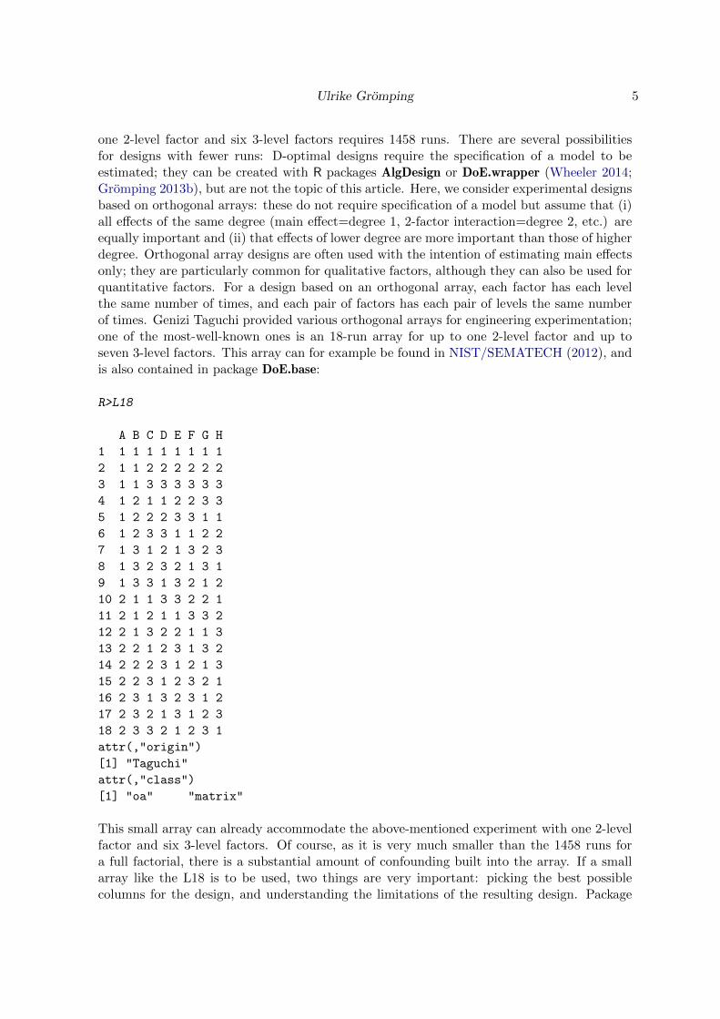
one 2-level factor and six 3-level factors requires 1458 runs. There are several possibilitiesfor designs with fewer runs: D-optimal designs require the specification of a model to beestimated; they can be created with R packages AlgDesign or DoE.wrapper (Wheeler 2014;Gromping 2013b), but are not the topic of this article. Here, we consider experimental designsbased on orthogonal arrays: these do not require specification of a model but assume that (i)all effects of the same degree (main effect=degree 1, 2-factor interaction=degree 2, etc.) areequally important and (ii) that effects of lower degree are more important than those of higherdegree. Orthogonal array designs are often used with the intention of estimating main effectsonly; they are particularly common for qualitative factors, although they can also be used forquantitative factors. For a design based on an orthogonal array, each factor has each levelthe same number of times, and each pair of factors has each pair of levels the same numberof times. Genizi Taguchi provided various orthogonal arrays for engineering experimentation;one of the most-well-known ones is an 18-run array for up to one 2-level factor and up toseven 3-level factors. This array can for example be found in NIST/SEMATECH (2012), andis also contained in package DoE.base:
R>L18
A B C D E F G H
1 1 1 1 1 1 1 1 1
2 1 1 2 2 2 2 2 2
3 1 1 3 3 3 3 3 3
4 1 2 1 1 2 2 3 3
5 1 2 2 2 3 3 1 1
6 1 2 3 3 1 1 2 2
7 1 3 1 2 1 3 2 3
8 1 3 2 3 2 1 3 1
9 1 3 3 1 3 2 1 2
10 2 1 1 3 3 2 2 1
11 2 1 2 1 1 3 3 2
12 2 1 3 2 2 1 1 3
13 2 2 1 2 3 1 3 2
14 2 2 2 3 1 2 1 3
15 2 2 3 1 2 3 2 1
16 2 3 1 3 2 3 1 2
17 2 3 2 1 3 1 2 3
18 2 3 3 2 1 2 3 1
attr(,"origin")
[1] "Taguchi"
attr(,"class")
[1] "oa" "matrix"
This small array can already accommodate the above-mentioned experiment with one 2-levelfactor and six 3-level factors. Of course, as it is very much smaller than the 1458 runs fora full factorial, there is a substantial amount of confounding built into the array. If a smallarray like the L18 is to be used, two things are very important: picking the best possiblecolumns for the design, and understanding the limitations of the resulting design. Package
6 R Package DoE.base
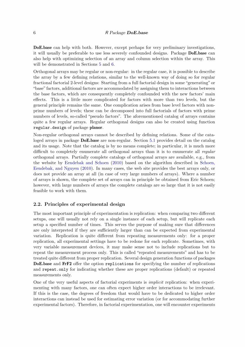
DoE.base can help with both. However, except perhaps for very preliminary investigations,it will usually be preferable to use less severely confounded designs. Package DoE.base canalso help with optimizing selection of an array and column selection within the array. Thiswill be demonstrated in Sections 5 and 6.
Orthogonal arrays may be regular or non-regular: in the regular case, it is possible to describethe array by a few defining relations, similar to the well-known way of doing so for regularfractional factorial 2-level designs: Starting from a full factorial design in some“generating”or“base” factors, additional factors are accommodated by assigning them to interactions betweenthe base factors, which are consequently completely confounded with the new factors’ maineffects. This is a little more complicated for factors with more than two levels, but thegeneral principle remains the same. One complication arises from base level factors with non-prime numbers of levels; these can be decomposed into full factorials of factors with primenumbers of levels, so-called “pseudo factors”. The aforementioned catalog of arrays containsquite a few regular arrays. Regular orthogonal designs can also be created using functionregular.design of package planor.
Non-regular orthogonal arrays cannot be described by defining relations. Some of the cata-loged arrays in package DoE.base are non-regular. Section 5.1 provides detail on the catalogand its usage. Note that the catalog is by no means complete; in particular, it is much moredifficult to completely enumerate all orthogonal arrays than it is to enumerate all regularorthogonal arrays. Partially complete catalogs of orthogonal arrays are available, e.g., fromthe website by Eendebak and Schoen (2010) based on the algorithm described in Schoen,Eendebak, and Nguyen (2010). In many cases, the web site provides the best arrays only, ordoes not provide an array at all (in case of very large numbers of arrays). Where a numberof arrays is shown, the complete set of arrays can in principle be obtained from Eric Schoen;however, with large numbers of arrays the complete catalogs are so large that it is not easilyfeasible to work with them.
2.2. Principles of experimental design
The most important principle of experimentation is replication: when comparing two differentsetups, one will usually not rely on a single instance of each setup, but will replicate eachsetup a specified number of times. This serves the purpose of making sure that differencesare only interpreted if they are sufficiently larger than can be expected from experimentalvariation. Replication is quite different from repeating measurements only: for a properreplication, all experimental settings have to be redone for each replicate. Sometimes, withvery variable measurement devices, it may make sense not to include replications but torepeat the measurement process only. This is called “repeated measurements” and has to betreated quite different from proper replication. Several design generation functions of packagesDoE.base and FrF2 offer the option replications for specifying the number of replicationsand repeat.only for indicating whether these are proper replications (default) or repeatedmeasurements only.
One of the very useful aspects of factorial experiments is implicit replication: when experi-menting with many factors, one can often expect higher order interactions to be irrelevant.If this is the case, the degrees of freedom that would have to be dedicated to higher orderinteractions can instead be used for estimating error variation (or for accommodating furtherexperimental factors). Therefore, in factorial experimentation, one will encounter experiments
Ulrike Gromping 7
without replicated runs.
A further important principle is blocking, which can be used to control for known influentialfactors that are not of interest in themselves, like batch-to-batch variation. For an orthogonalarray design, one can simply include the block factor as an additional factor and thus has tofind an array of the desired structure. A full factorial design can be blocked without increasingthe number of runs, by allocating the degrees of freedom for the block factor to portions frominteraction effects. This functionality is implemented in function fac.design (see Section 4).
Randomization means that the experimental runs are conducted in random order; it is asafeguard against bias from unknown influences. If the run order is completely randomized,all experimental runs can be treated as independent observations, and there is little risk ofsystematic bias from experimental order or unknown factors related to experimental orderor time. In real life, there are sometimes so-called randomization restrictions; for example,experimental runs may be randomized within each block only. Function fac.design allowsrandomization within blocks, while designs created with function oa.design have to be re-randomized with function rerandomize.design for using one of the factors as a block factor.
Whenever proper replication is used, package DoE.base separately randomizes each replicationas though it were a block; however, it does not include a block factor for the replications. Userswho want to include a block factor for replications in the analysis can obtain such a factorusing the function getblock. Users who want to change the randomization, i.e., randomize allreplications together instead of in separate blocks, can use the function rerandomize.design.Using the “[” method for the class design, users can also reorder a design according toa randomization scheme that has been worked out outside of R. Of course, whenever therandomization involves non-trivial restrictions like randomizing in meaningful blocks, theanalysis has to be conducted accordingly.
3. General orthogonal arrays
This section provides the mathematical background for general orthogonal arrays, as far asit can be helpful for using the orthogonal arrays available in R package DoE.base.
3.1. Terminology for orthogonal arrays
An array in the sense of this article is a rectangular table of numbers with n rows andk columns, like the L18 shown on p. 5. The rows correspond to experimental runs, thecolumns to experimental factors. In the cataloged arrays in DoE.base, the levels of an l-level factor are denoted by the numbers 1...l. An array becomes an experimental design byallocating numbers to factor levels. The array is orthogonal, i.e., an OA, if for each pair ofcolumns each combination of levels occurs equally often. If this is the case, main effects of allfactors can be estimated separately from each other (provided, no higher order effects are inthe model).
An OA is said to be of strength s, if each combination of levels occurs equally often foreach subset of s columns. Thus, each OA is at least of strength 2. Strength of an OA isdirectly related to resolution of an array: resolution, denoted by roman numerals, is alwaysone higher than the strength, i.e., strength 2 arrays are of resolution III and so forth. Foran array of resolution III, main effects are not aliased with main effects, but can be aliasedwith 2-factor interactions (three factors involved); for an array of resolution IV, main effects
8 R Package DoE.base
are not aliased with 2-factor interactions, but can be aliased with 3-factor interactions, while2-factor interactions can be aliased with other 2-factor interactions (four factors involved).This notion is well-known for regular fractional factorial 2-level designs, and is completelyanalogous for non-regular designs and for designs with factors at more than 2 levels or inmixed level situations. Note that a full factorial in k factors has strength k.
3.2. Generalized word length pattern and refinements
Xu and Wu (2001) introduced the generalized word length pattern (GWLP) for general or-thogonal arrays. It is an extension of the well-known word length pattern (WLP) for regularfractional factorial 2-level designs: in the latter, one starts out with a set of base factors andallocates additional factors to interactions among these (the generating contrasts). Codingall main effects model matrix columns with “-1” (one level) and “+1” (the other level), thisway of design generation causes products of model matrix columns to be either half “-1” andhalf “+1”, or constant columns. Factors, whose product of model matrix columns yields aconstant column, form a “word” together. The word length pattern is a frequency table ofword lengths. For regular fractional factorial 2-level designs, each group of c factors eitherdoes or does not form a word, i.e., contributes one or zero to the count for words of length c.This results in a word length pattern with only integer entries.
In general, partial aliasing is possible. Even if there are only 2-level factors, e.g., in a Plackett-Burman design (Plackett and Burman 1946), a set of factors can contribute a fraction of aword to the GWLP count for the respective word length. Consequently, GWLP entries neednot be integers. For example, the GWLP of the L18 is
R>GWLP(L18)
0 1 2 3 4 5 6 7 8
1.0 0.0 0.0 28.0 52.5 52.5 70.0 33.0 6.0
The GWLP is denoted as A0, A1, A2, A3, ..., with Ac the number of generalized words oflength c. The entry “1” for A0 is generic and does not indicate confounding. The GWLPfor orthogonal arrays and designs based on them is usually presented starting with A3, sinceorthogonality implies absence of words of lengths one or two. The GWLP coincides with theWLP for regular fractional factorial 2-level designs; for details, consult Xu and Wu (2001)themselves or Gromping (2011a) for a more accessible account. The concepts of strength andresolution directly relate to the (G)WLP: the shortest word length with a non-zero countis the resolution of the design, the longest word length with a zero count is the strength.Hence, the L18 has resolution III and strength 2. Note that it is not adequate to use the term“generalized resolution” here, because that term is already in use for a different concept thatis also implemented in package DoE.base (see below).
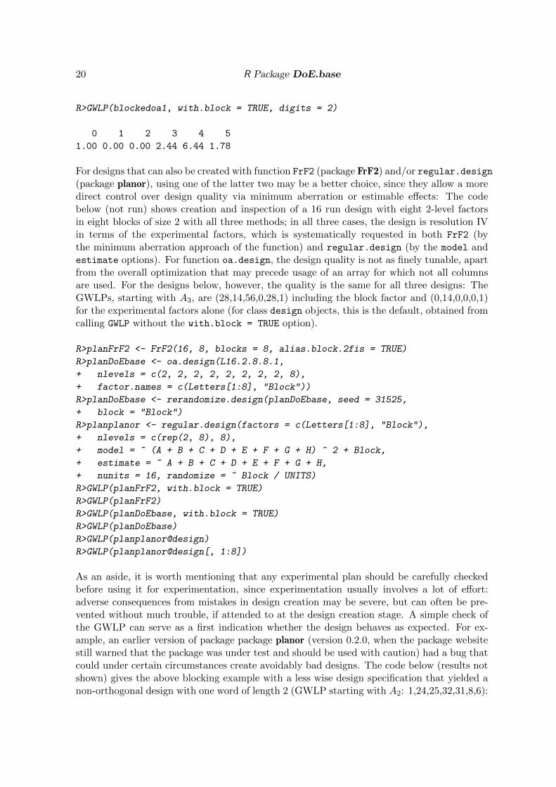
The number of generalized words of length c is the sum over contributions from all sets ofc factors. For a set of R factors with l1...lR levels in a resolution R design (equivalent tos + 1 factors in a strength s design), Gromping and Xu (2014) have shown an upper boundfor the contribution to the count AR to be min((l1 − 1), ..., (lR − 1)), i.e., the upper boundfor the number of generalized words in a set of R factors depends on the pattern of levels inthe set and is given by the main effect degrees of freedom for the factor with the fewest levels
Ulrike Gromping 9
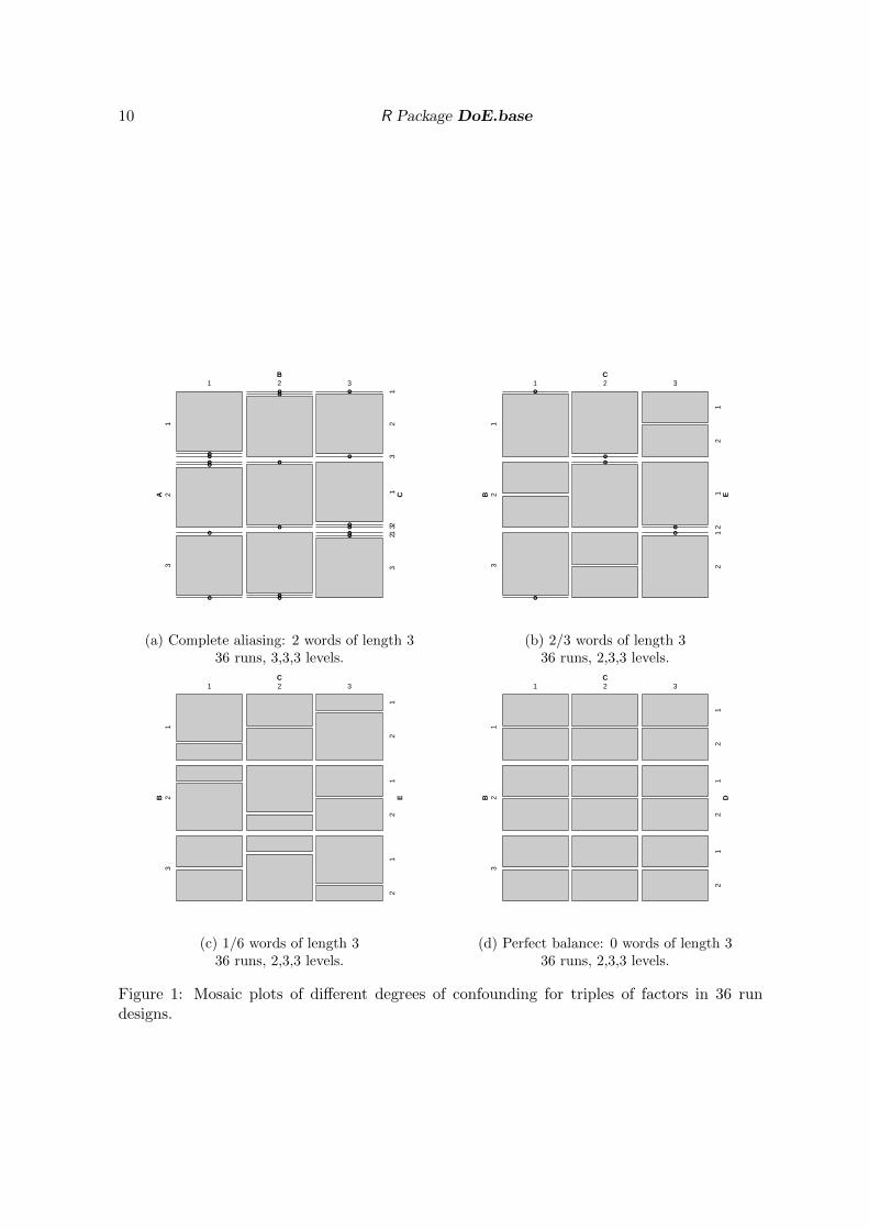
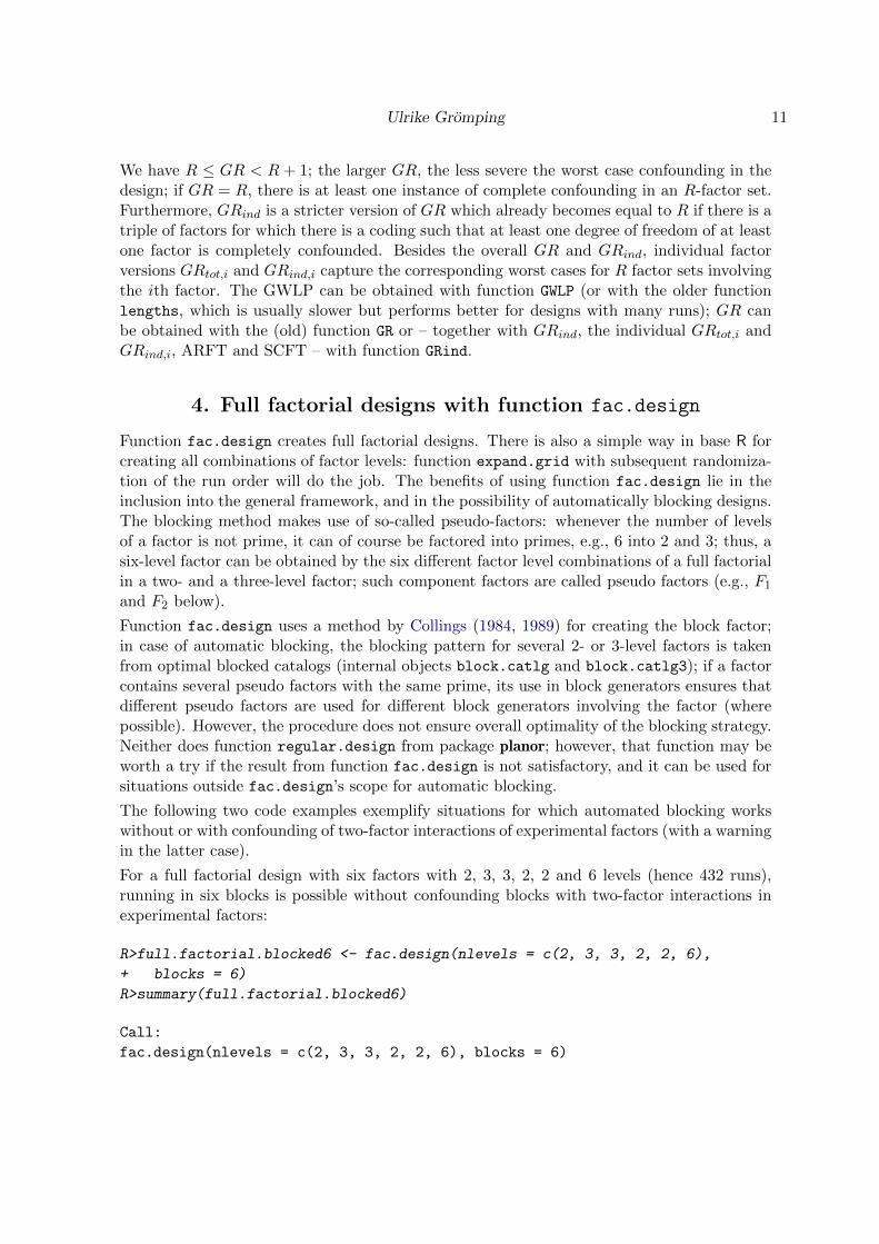
(the analogous result for symmetric designs was shown earlier by Xu, Cheng, and Wu 2004).Furthermore, Gromping and Xu (2014) provided a statistical rationale for the contributionsof sets of R factors to AR in resolution R designs, i.e., the building blocks for the number ofshortest words: each R-set contribution can be seen as the sum of R2-values from linear modelsexplaining orthogonal contrast columns for any one of the R factors by a full model in theother R−1 factors (provided the factor to be explained has orthogonally coded model matrixcolumns; otherwise, R2 values have to be replaced by squared canonical correlations). Thus,the number of shortest words measures the extent of worst-case confounding in a plausibleway. It is therefore particularly instructive to study R factor sets in resolution R designs.Based on these, Figure 1 illustrates the meaning of words in an informal sense, using mosaicplots as proposed in Gromping (2014a). The most severe imbalance is shown in plot (a)of the figure: the factor level combination of any pair of factors completely determines thelevel of the third factor. This is a resolution III regular array, for which each main effect isconfounded by the two-factor interaction of the other two factors. This is reflected in thenumber of words, which coincides with the aforementioned upper bound. The plot shows atriple from the array L36.2.16.3.4 from package DoE.base; an identical plot can be producedfrom columns 2, 4 and 5 of the well-known Taguchi L18 shown on p. 5.
The factor set of Figure 1 (a) attains its upper bound for the number of generalized words.For the other factor sets shown in Figure 1, the upper bound is one because of one degree offreedom only for the 2-level factor in the set. However, with a 2-level and two 3-level factorsin an orthogonal array, this upper bound cannot be attained. The upper bound can only beattained if the smallest number of levels is a divisor of all the other numbers of levels, whichis for example the case in symmetric designs. In summary, the figure illustrates that morewords are related to less balance.
The GWLP can be used for selecting a best design by comparing designs with respect totheir so-called aberration: a design is better than another one, if it has higher resolution; incase of equal resolution, a design has smaller aberration, if its number of shortest words issmaller, in case of ties, successively considering longer words until a difference is encountered.If this principle is applied to a complete set of possible designs, the best design is said to have“generalized minimum aberration” (GMA).
Over and above the GWLP, package DoE.base allows to look at individual R-factor set con-founding through mosaic plots (Gromping 2014a), like the ones shown in Figure 1, and pro-vides an overview of the confounding in R-factor projections through projection frequencytables (functions P3.3 or P4.4), average R2 frequency tables (ARFT) and squared canonicalcorrelation frequency tables (SCFT); the latter are based on the results by Gromping andXu (2014) and detailed in Gromping (2013a). Sometimes, several designs that have GMAcan be distinguished further by the more detailed criteria. Gromping and Xu (2014) alsointroduced a generalization of the generalized resolution GR as proposed by Deng and Tang(1999): GR refines the resolution R by indicating the distance from complete confounding.
10 R Package DoE.base
●●
●●
●
●
●●
●
●●●
●
●●●
●●
B
A C
3 321
2
321
1
1 2 33
21
(a) Complete aliasing: 2 words of length 336 runs, 3,3,3 levels.
●
●
●
●
●
●
C
B E
3 21
2
21
1
1 2 3
21
(b) 2/3 words of length 336 runs, 2,3,3 levels.
C
B E
3
21
2
21
1
1 2 3
21
(c) 1/6 words of length 336 runs, 2,3,3 levels.
C
B D
3
21
2
21
1
1 2 3
21
(d) Perfect balance: 0 words of length 336 runs, 2,3,3 levels.
Figure 1: Mosaic plots of different degrees of confounding for triples of factors in 36 rundesigns.
Ulrike Gromping 11
We have R ≤ GR < R + 1; the larger GR, the less severe the worst case confounding in thedesign; if GR = R, there is at least one instance of complete confounding in an R-factor set.Furthermore, GRind is a stricter version of GR which already becomes equal to R if there is atriple of factors for which there is a coding such that at least one degree of freedom of at leastone factor is completely confounded. Besides the overall GR and GRind, individual factorversions GRtot,i and GRind,i capture the corresponding worst cases for R factor sets involvingthe ith factor. The GWLP can be obtained with function GWLP (or with the older functionlengths, which is usually slower but performs better for designs with many runs); GR canbe obtained with the (old) function GR or – together with GRind, the individual GRtot,i andGRind,i, ARFT and SCFT – with function GRind.
4. Full factorial designs with function fac.design
Function fac.design creates full factorial designs. There is also a simple way in base R forcreating all combinations of factor levels: function expand.grid with subsequent randomiza-tion of the run order will do the job. The benefits of using function fac.design lie in theinclusion into the general framework, and in the possibility of automatically blocking designs.The blocking method makes use of so-called pseudo-factors: whenever the number of levelsof a factor is not prime, it can of course be factored into primes, e.g., 6 into 2 and 3; thus, asix-level factor can be obtained by the six different factor level combinations of a full factorialin a two- and a three-level factor; such component factors are called pseudo factors (e.g., F1
and F2 below).
Function fac.design uses a method by Collings (1984, 1989) for creating the block factor;in case of automatic blocking, the blocking pattern for several 2- or 3-level factors is takenfrom optimal blocked catalogs (internal objects block.catlg and block.catlg3); if a factorcontains several pseudo factors with the same prime, its use in block generators ensures thatdifferent pseudo factors are used for different block generators involving the factor (wherepossible). However, the procedure does not ensure overall optimality of the blocking strategy.Neither does function regular.design from package planor; however, that function may beworth a try if the result from function fac.design is not satisfactory, and it can be used forsituations outside fac.design’s scope for automatic blocking.
The following two code examples exemplify situations for which automated blocking workswithout or with confounding of two-factor interactions of experimental factors (with a warningin the latter case).
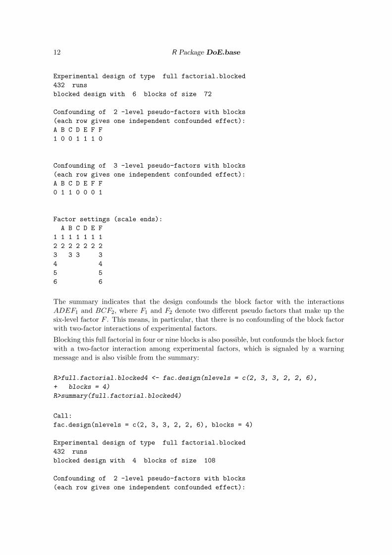
For a full factorial design with six factors with 2, 3, 3, 2, 2 and 6 levels (hence 432 runs),running in six blocks is possible without confounding blocks with two-factor interactions inexperimental factors:
R>full.factorial.blocked6 <- fac.design(nlevels = c(2, 3, 3, 2, 2, 6),
+ blocks = 6)
R>summary(full.factorial.blocked6)
Call:
fac.design(nlevels = c(2, 3, 3, 2, 2, 6), blocks = 6)
12 R Package DoE.base
Experimental design of type full factorial.blocked
432 runs
blocked design with 6 blocks of size 72
Confounding of 2 -level pseudo-factors with blocks
(each row gives one independent confounded effect):
A B C D E F F
1 0 0 1 1 1 0
Confounding of 3 -level pseudo-factors with blocks
(each row gives one independent confounded effect):
A B C D E F F
0 1 1 0 0 0 1
Factor settings (scale ends):
A B C D E F
1 1 1 1 1 1 1
2 2 2 2 2 2 2
3 3 3 3
4 4
5 5
6 6
The summary indicates that the design confounds the block factor with the interactionsADEF1 and BCF2, where F1 and F2 denote two different pseudo factors that make up thesix-level factor F . This means, in particular, that there is no confounding of the block factorwith two-factor interactions of experimental factors.
Blocking this full factorial in four or nine blocks is also possible, but confounds the block factorwith a two-factor interaction among experimental factors, which is signaled by a warningmessage and is also visible from the summary:
R>full.factorial.blocked4 <- fac.design(nlevels = c(2, 3, 3, 2, 2, 6),
+ blocks = 4)
R>summary(full.factorial.blocked4)
Call:
fac.design(nlevels = c(2, 3, 3, 2, 2, 6), blocks = 4)
Experimental design of type full factorial.blocked
432 runs
blocked design with 4 blocks of size 108
Confounding of 2 -level pseudo-factors with blocks
(each row gives one independent confounded effect):
Ulrike Gromping 13
A B C D E F F
[1,] 1 0 0 0 1 1 0
[2,] 0 0 0 1 1 1 0
[3,] 1 0 0 1 0 0 0
Factor settings (scale ends):
A B C D E F
1 1 1 1 1 1 1
2 2 2 2 2 2 2
3 3 3 3
4 4
5 5
6 6
The function allows automatic blocking for the most frequent situations, where most primefactors are two and three, and only single prime (pseudo) factors are larger than three; thereis also a limit on the number of 2- and 3-level factors (see the package manual).
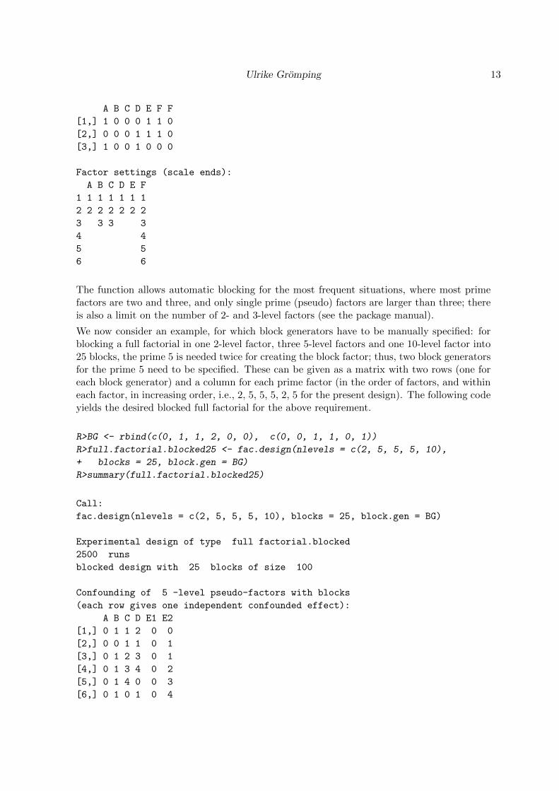
We now consider an example, for which block generators have to be manually specified: forblocking a full factorial in one 2-level factor, three 5-level factors and one 10-level factor into25 blocks, the prime 5 is needed twice for creating the block factor; thus, two block generatorsfor the prime 5 need to be specified. These can be given as a matrix with two rows (one foreach block generator) and a column for each prime factor (in the order of factors, and withineach factor, in increasing order, i.e., 2, 5, 5, 5, 2, 5 for the present design). The following codeyields the desired blocked full factorial for the above requirement.
R>BG <- rbind(c(0, 1, 1, 2, 0, 0), c(0, 0, 1, 1, 0, 1))
R>full.factorial.blocked25 <- fac.design(nlevels = c(2, 5, 5, 5, 10),
+ blocks = 25, block.gen = BG)
R>summary(full.factorial.blocked25)
Call:
fac.design(nlevels = c(2, 5, 5, 5, 10), blocks = 25, block.gen = BG)
Experimental design of type full factorial.blocked
2500 runs
blocked design with 25 blocks of size 100
Confounding of 5 -level pseudo-factors with blocks
(each row gives one independent confounded effect):
A B C D E1 E2
[1,] 0 1 1 2 0 0
[2,] 0 0 1 1 0 1
[3,] 0 1 2 3 0 1
[4,] 0 1 3 4 0 2
[5,] 0 1 4 0 0 3
[6,] 0 1 0 1 0 4
14 R Package DoE.base
Factor settings (scale ends):
A B C D E
1 1 1 1 1 1
2 2 2 2 2 2
3 3 3 3 3
4 4 4 4 4
5 5 5 5 5
6 6
7 7
8 8
9 9
10 10
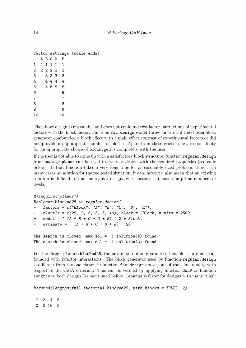
The above design is reasonable and does not confound two-factor interactions of experimentalfactors with the block factor. Function fac.design would throw an error, if the chosen blockgenerator confounded a block effect with a main effect contrast of experimental factors or didnot provide an appropriate number of blocks. Apart from these gross issues, responsibilityfor an appropriate choice of block.gen is completely with the user.
If the user is not able to come up with a satisfactory block structure, function regular.design
from package planor can be used to create a design with the required properties (see codebelow). If that function takes a very long time for a reasonably-sized problem, there is inmany cases no solution for the requested situation; it can, however, also mean that an existingsolution is difficult to find for regular designs with factors that have non-prime numbers oflevels.
R>require("planor")
R>planor.blocked25 <- regular.design(
+ factors = c("Block", "A", "B", "C", "D", "E"),
+ nlevels = c(25, 2, 5, 5, 5, 10), block = ~Block, nunits = 2500,
+ model = ~ (A + B + C + D + E) ^ 2 + Block,
+ estimate = ~ (A + B + C + D + E) ^ 2)
The search is closed: max.sol = 1 solution(s) found
The search is closed: max.sol = 1 solution(s) found
For the design planor.blocked25, the estimate option guarantees that blocks are not con-founded with 2-factor interactions. The block generator used by function regular.design
is different from the one chosen in function fac.design above, but of the same quality withrespect to the GMA criterion. This can be verified by applying function GWLP or functionlengths to both designs (as mentioned before, lengths is faster for designs with many runs):
R>round(lengths(full.factorial.blocked25, with.blocks = TRUE), 2)
2 3 4 5
0 0 16 8
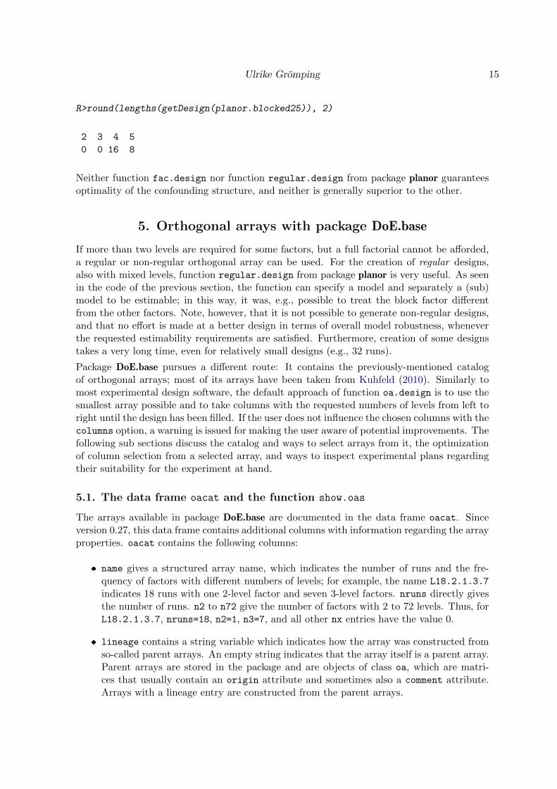
Ulrike Gromping 15
R>round(lengths(getDesign(planor.blocked25)), 2)
2 3 4 5
0 0 16 8
Neither function fac.design nor function regular.design from package planor guaranteesoptimality of the confounding structure, and neither is generally superior to the other.
5. Orthogonal arrays with package DoE.base
If more than two levels are required for some factors, but a full factorial cannot be afforded,a regular or non-regular orthogonal array can be used. For the creation of regular designs,also with mixed levels, function regular.design from package planor is very useful. As seenin the code of the previous section, the function can specify a model and separately a (sub)model to be estimable; in this way, it was, e.g., possible to treat the block factor differentfrom the other factors. Note, however, that it is not possible to generate non-regular designs,and that no effort is made at a better design in terms of overall model robustness, wheneverthe requested estimability requirements are satisfied. Furthermore, creation of some designstakes a very long time, even for relatively small designs (e.g., 32 runs).
Package DoE.base pursues a different route: It contains the previously-mentioned catalogof orthogonal arrays; most of its arrays have been taken from Kuhfeld (2010). Similarly tomost experimental design software, the default approach of function oa.design is to use thesmallest array possible and to take columns with the requested numbers of levels from left toright until the design has been filled. If the user does not influence the chosen columns with thecolumns option, a warning is issued for making the user aware of potential improvements. Thefollowing sub sections discuss the catalog and ways to select arrays from it, the optimizationof column selection from a selected array, and ways to inspect experimental plans regardingtheir suitability for the experiment at hand.
5.1. The data frame oacat and the function show.oas
The arrays available in package DoE.base are documented in the data frame oacat. Sinceversion 0.27, this data frame contains additional columns with information regarding the arrayproperties. oacat contains the following columns:
� name gives a structured array name, which indicates the number of runs and the fre-quency of factors with different numbers of levels; for example, the name L18.2.1.3.7
indicates 18 runs with one 2-level factor and seven 3-level factors. nruns directly givesthe number of runs. n2 to n72 give the number of factors with 2 to 72 levels. Thus, forL18.2.1.3.7, nruns=18, n2=1, n3=7, and all other nx entries have the value 0.
� lineage contains a string variable which indicates how the array was constructed fromso-called parent arrays. An empty string indicates that the array itself is a parent array.Parent arrays are stored in the package and are objects of class oa, which are matri-ces that usually contain an origin attribute and sometimes also a comment attribute.Arrays with a lineage entry are constructed from the parent arrays.

16 R Package DoE.base
� Logical columns indicate a full factorial array (ff), an array with only squared canonicalcorrelations 0 and 1 (regular), and an array with only average R2 values 0 and 1(regular.strict; these can only be fixed level arrays). Note that the squared canonicalcorrelations and average R2 values currently refer to R factor projections, where R isthe resolution of the entire array; an array that exhibits regular behavior for all suchprojections might still be non-regular when considering projections onto larger numbersof factors. Thus, the regularity indicator columns might change with future packageversions.
� Column SCones contains the number of squared canonical correlations that are one.
� Columns GR and GRind contain the GR and GRind values, respectively.
� Columns maxAR and maxSC contain the maximum average R2 or squared canonical cor-relation, respectively.
� Column dfe provides the number of error degrees of freedom, if the all columns of thearray are used.
� Columns A3 to A8 provide the numbers of generalized words of lengths 3 to 8. (Thereare no words of shorter lengths, of course.)
It is possible to use the data frame oacat directly for inspecting which arrays of a certainnature are available, for example for finding 32 run arrays which are regular but not strictlyregular:
R>oacat$name[oacat$nruns==32 & oacat$regular & !oacat$regular.strict]
[1] "L32.2.28.4.1" "L32.2.25.4.2" "L32.2.24.8.1"
[4] "L32.2.22.4.3" "L32.2.21.4.1.8.1" "L32.2.19.4.4"
[7] "L32.2.18.4.2.8.1" "L32.2.16.4.5" "L32.2.16.16.1"
[10] "L32.2.15.4.3.8.1" "L32.2.13.4.6" "L32.2.12.4.4.8.1"
[13] "L32.2.10.4.7" "L32.2.9.4.5.8.1" "L32.2.7.4.8"
[16] "L32.2.6.4.6.8.1" "L32.2.4.4.9" "L32.2.3.4.7.8.1"
[19] "L32.4.8.8.1"
The author prefers non-regular arrays for many situations, at least for the creation of screeningdesigns. Looking at regular arrays in package DoE.base may nevertheless be of interest, iffunction regular.design of package planor runs for a long time without indicating failure fora run size that is in the scope of package DoE.base: if there is a regular array of the desired sizein DoE.base, this array can be inspected and perhaps used after column optimization (seenext section). Also, in principle, function regular.design can be expected to eventuallysucceed, unless estimability requirements make the existing array unsuitable. However, noteagain that the value TRUE in column regular or even regular.strict of oacat refers toprojections onto R factors with R the array’s resolution and does not guarantee regularityof the entire array. For example, the array L24.2.12.12.1 has only regular three-factorprojections (full factorial for triples of 2-level factors, confounded for triples with the 12-levelfactor), but non-regular four-factor projections (for quadruples of 2-level factors).
Ulrike Gromping 17
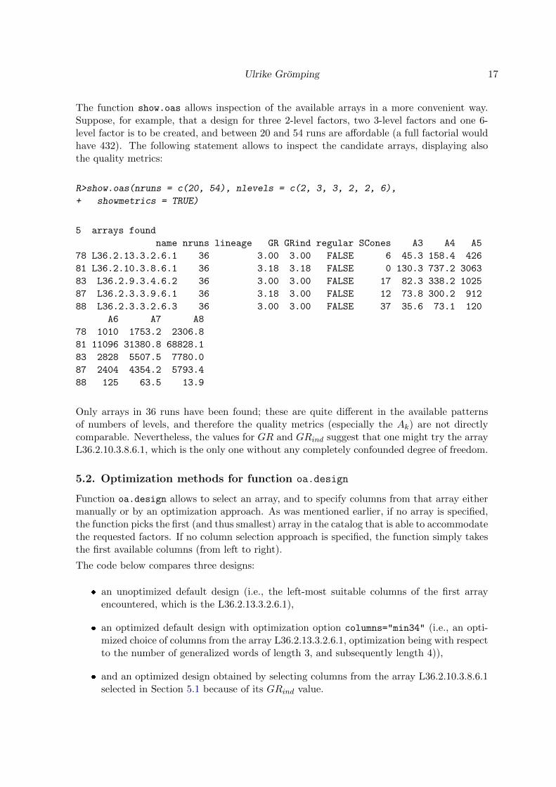
The function show.oas allows inspection of the available arrays in a more convenient way.Suppose, for example, that a design for three 2-level factors, two 3-level factors and one 6-level factor is to be created, and between 20 and 54 runs are affordable (a full factorial wouldhave 432). The following statement allows to inspect the candidate arrays, displaying alsothe quality metrics:
R>show.oas(nruns = c(20, 54), nlevels = c(2, 3, 3, 2, 2, 6),
+ showmetrics = TRUE)
5 arrays found
name nruns lineage GR GRind regular SCones A3 A4 A5
78 L36.2.13.3.2.6.1 36 3.00 3.00 FALSE 6 45.3 158.4 426
81 L36.2.10.3.8.6.1 36 3.18 3.18 FALSE 0 130.3 737.2 3063
83 L36.2.9.3.4.6.2 36 3.00 3.00 FALSE 17 82.3 338.2 1025
87 L36.2.3.3.9.6.1 36 3.18 3.00 FALSE 12 73.8 300.2 912
88 L36.2.3.3.2.6.3 36 3.00 3.00 FALSE 37 35.6 73.1 120
A6 A7 A8
78 1010 1753.2 2306.8
81 11096 31380.8 68828.1
83 2828 5507.5 7780.0
87 2404 4354.2 5793.4
88 125 63.5 13.9
Only arrays in 36 runs have been found; these are quite different in the available patternsof numbers of levels, and therefore the quality metrics (especially the Ak) are not directlycomparable. Nevertheless, the values for GR and GRind suggest that one might try the arrayL36.2.10.3.8.6.1, which is the only one without any completely confounded degree of freedom.
5.2. Optimization methods for function oa.design
Function oa.design allows to select an array, and to specify columns from that array eithermanually or by an optimization approach. As was mentioned earlier, if no array is specified,the function picks the first (and thus smallest) array in the catalog that is able to accommodatethe requested factors. If no column selection approach is specified, the function simply takesthe first available columns (from left to right).
The code below compares three designs:
� an unoptimized default design (i.e., the left-most suitable columns of the first arrayencountered, which is the L36.2.13.3.2.6.1),
� an optimized default design with optimization option columns="min34" (i.e., an opti-mized choice of columns from the array L36.2.13.3.2.6.1, optimization being with respectto the number of generalized words of length 3, and subsequently length 4)),
� and an optimized design obtained by selecting columns from the array L36.2.10.3.8.6.1selected in Section 5.1 because of its GRind value.
18 R Package DoE.base
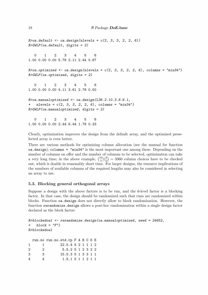
R>oa.default <- oa.design(nlevels = c(2, 3, 3, 2, 2, 6))
R>GWLP(oa.default, digits = 2)
0 1 2 3 4 5 6
1.00 0.00 0.00 5.78 2.11 2.44 0.67
R>oa.optimized <- oa.design(nlevels = c(2, 3, 3, 2, 2, 6), columns = "min34")
R>GWLP(oa.optimized, digits = 2)
0 1 2 3 4 5 6
1.00 0.00 0.00 4.11 3.61 2.78 0.50
R>oa.manualoptimized <- oa.design(L36.2.10.3.8.6.1,
+ nlevels = c(2, 3, 3, 2, 2, 6), columns = "min34")
R>GWLP(oa.manualoptimized, digits = 2)
0 1 2 3 4 5 6
1.00 0.00 0.00 2.44 6.44 1.78 0.33
Clearly, optimization improves the design from the default array, and the optimized prese-lected array is even better.
There are various methods for optimizing column allocation (see the manual for functionoa.design); columns = "min34" is the most important one among these. Depending on thenumber of columns on offer and the number of columns to be selected, optimization can takea very long time; in the above example,
(103
)(82
)= 3360 column choices have to be checked
out, which is doable in reasonably short time. For larger designs, the resource implications ofthe numbers of available columns of the required lengths may also be considered in selectingan array to use.
5.3. Blocking general orthogonal arrays
Suppose a design with the above factors is to be run, and the 6-level factor is a blockingfactor. In that case, the design should be randomized such that runs are randomized withinblocks. Function oa.design does not directly allow to block randomization. However, thefunction rerandomize.design allows a post-hoc randomization within a single design factordeclared as the block factor:
R>blockedoa1 <- rerandomize.design(oa.manualoptimized, seed = 24652,
+ block = "F")
R>blockedoa1
run.no run.no.std.rp F A B C D E
1 1 22.5.4 5 2 1 1 1 2
2 2 5.5.2 5 1 2 3 2 2
3 3 15.5.3 5 1 3 3 1 1
4 4 1.5.1 5 1 1 2 1 1
Ulrike Gromping 19
5 5 35.5.6 5 2 2 1 2 1
6 6 33.5.5 5 2 3 2 2 2
run.no run.no.std.rp F A B C D E
7 7 32.3.5 3 2 2 1 2 2
8 8 14.3.3 3 1 2 2 1 1
9 9 34.3.6 3 2 1 3 2 1
10 10 4.3.2 3 1 1 2 2 2
11 11 3.3.1 3 1 3 1 1 1
12 12 24.3.4 3 2 3 3 1 2
run.no run.no.std.rp F A B C D E
13 13 18.4.3 4 1 3 3 2 2
14 14 26.4.5 4 2 2 2 2 1
15 15 30.4.6 4 2 3 1 1 1
16 16 11.4.2 4 1 2 1 1 2
17 17 7.4.1 4 1 1 3 2 1
18 18 19.4.4 4 2 1 2 1 2
run.no run.no.std.rp F A B C D E
19 19 10.2.2 2 1 1 3 1 2
20 20 21.2.4 2 2 3 1 1 2
21 21 29.2.6 2 2 2 3 1 1
22 22 17.2.3 2 1 2 2 2 2
23 23 9.2.1 2 1 3 2 2 1
24 24 25.2.5 2 2 1 1 2 1
run.no run.no.std.rp F A B C D E
25 25 20.6.4 6 2 2 3 1 2
26 26 16.6.3 6 1 1 1 2 2
27 27 8.6.1 6 1 2 1 2 1
28 28 12.6.2 6 1 3 2 1 2
29 29 28.6.6 6 2 1 2 1 1
30 30 27.6.5 6 2 3 3 2 1
run.no run.no.std.rp F A B C D E
31 31 31.1.5 1 2 1 3 2 2
32 32 36.1.6 1 2 3 2 2 1
33 33 13.1.3 1 1 1 1 1 1
34 34 2.1.1 1 1 2 3 1 1
35 35 23.1.4 1 2 2 2 1 2
36 36 6.1.2 1 1 3 1 2 2
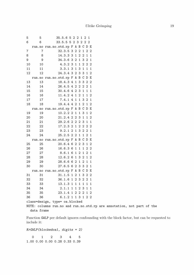
class=design, type= oa.blocked
NOTE: columns run.no and run.no.std.rp are annotation, not part of the
data frame
Function GWLP per default ignores confounding with the block factor, but can be requested toinclude it:
R>GWLP(blockedoa1, digits = 2)
0 1 2 3 4 5
1.00 0.00 0.00 0.28 0.33 0.39
20 R Package DoE.base
R>GWLP(blockedoa1, with.block = TRUE, digits = 2)
0 1 2 3 4 5
1.00 0.00 0.00 2.44 6.44 1.78
For designs that can also be created with function FrF2 (package FrF2) and/or regular.design(package planor), using one of the latter two may be a better choice, since they allow a moredirect control over design quality via minimum aberration or estimable effects: The codebelow (not run) shows creation and inspection of a 16 run design with eight 2-level factorsin eight blocks of size 2 with all three methods; in all three cases, the design is resolution IVin terms of the experimental factors, which is systematically requested in both FrF2 (bythe minimum aberration approach of the function) and regular.design (by the model andestimate options). For function oa.design, the design quality is not as finely tunable, apartfrom the overall optimization that may precede usage of an array for which not all columnsare used. For the designs below, however, the quality is the same for all three designs: TheGWLPs, starting with A3, are (28,14,56,0,28,1) including the block factor and (0,14,0,0,0,1)for the experimental factors alone (for class design objects, this is the default, obtained fromcalling GWLP without the with.block = TRUE option).
R>planFrF2 <- FrF2(16, 8, blocks = 8, alias.block.2fis = TRUE)
R>planDoEbase <- oa.design(L16.2.8.8.1,
+ nlevels = c(2, 2, 2, 2, 2, 2, 2, 2, 8),
+ factor.names = c(Letters[1:8], "Block"))
R>planDoEbase <- rerandomize.design(planDoEbase, seed = 31525,
+ block = "Block")
R>planplanor <- regular.design(factors = c(Letters[1:8], "Block"),
+ nlevels = c(rep(2, 8), 8),
+ model = ~ (A + B + C + D + E + F + G + H) ^ 2 + Block,
+ estimate = ~ A + B + C + D + E + F + G + H,
+ nunits = 16, randomize = ~ Block / UNITS)
R>GWLP(planFrF2, with.block = TRUE)
R>GWLP(planFrF2)
R>GWLP(planDoEbase, with.block = TRUE)
R>GWLP(planDoEbase)
R>GWLP(planplanor@design)
R>GWLP(planplanor@design[, 1:8])
As an aside, it is worth mentioning that any experimental plan should be carefully checkedbefore using it for experimentation, since experimentation usually involves a lot of effort:adverse consequences from mistakes in design creation may be severe, but can often be pre-vented without much trouble, if attended to at the design creation stage. A simple check ofthe GWLP can serve as a first indication whether the design behaves as expected. For ex-ample, an earlier version of package package planor (version 0.2.0, when the package websitestill warned that the package was under test and should be used with caution) had a bug thatcould under certain circumstances create avoidably bad designs. The code below (results notshown) gives the above blocking example with a less wise design specification that yielded anon-orthogonal design with one word of length 2 (GWLP starting with A2: 1,24,25,32,31,8,6):
Ulrike Gromping 21
R>planoldplanor.bug <- regular.design(factors = c(Letters[1:8], "Block"),
+ nlevels = c(rep(2, 8), 8),
+ model = ~ A + B + C + D + E + F + G + H + Block,
+ estimate = ~ A + B + C+ D + E + F + G + H,
+ nunits = 16, randomize = ~ Block / UNITS)
R>GWLP(planoldplanor.bug@design)
R>plot(planor2design(planoldplanor.bug), select = "all2")
The plot command in the code above revealed that factor C was aliased with the Block factorfor the latter design, which explains the word of length 2. Such a design should of course notbe used. Let me emphasize that this example is not meant to imply that package planor isless trustworthy than other design creation packages but rather that a design should alwaysbe checked before using it for experimentation!
5.4. Inspection methods for factorial designs
This is a good place to exemplify further possibilities for design inspection. The functionnames for obtaining quality criteria were already mentioned in Section 3.2.
The function GRind calculates the metrics introduced by Gromping and Xu (2014) with theadditional detail proposed in Gromping (2013a). For example, the code below shows that theoptimized design based on the manually selected array has a clearly better overall behaviorregarding factor-specific worst case confounding (GRtot, i and GRind,i, see Section 3.2) thanthe optimized design based on the automatically selected first array:
R>GRind1 <- GRind(oa.optimized)
R>GRind2 <- GRind(oa.manualoptimized)
R>print(cbind(rep(c("oa.opimized", "oa.optimized2"), each = 2),
+ rbind(GRind1$GR.i, GRind2$GR.i)), quote = FALSE)
A B C D E F
GRtot.i oa.opimized 3.667 3 3 3.423 3.423 3.368
GRind.i oa.opimized 3.667 3 3 3.423 3.423 3
GRtot.i oa.optimized2 3.184 3.5 3.423 3.423 3.667 3.635
GRind.i oa.optimized2 3.184 3.5 3.423 3.423 3.667 3.423
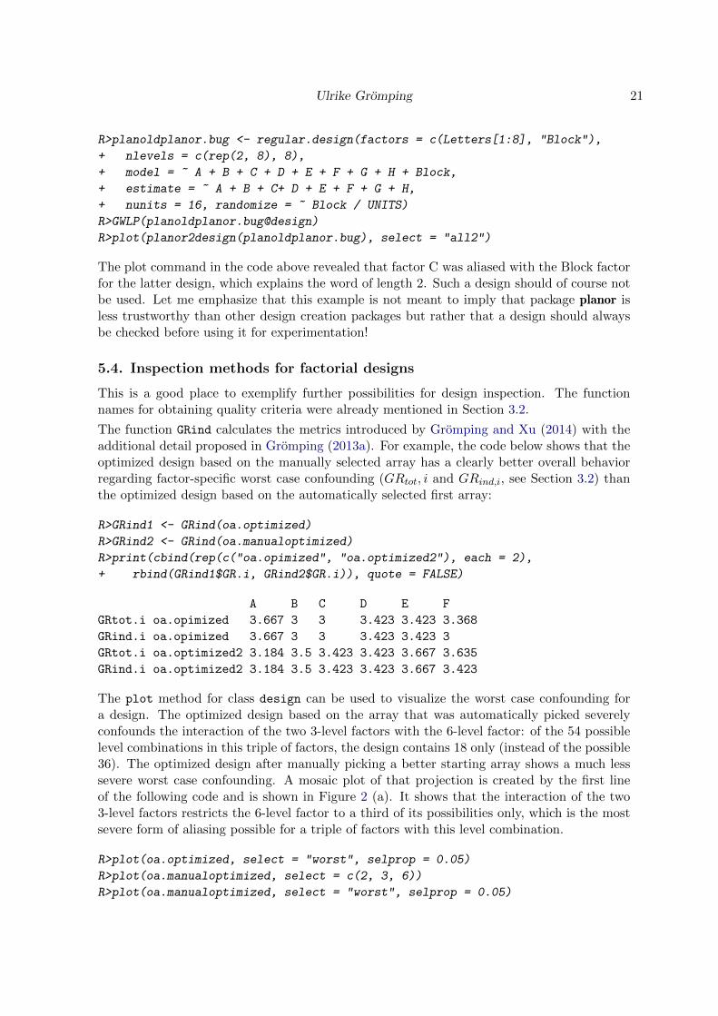
The plot method for class design can be used to visualize the worst case confounding fora design. The optimized design based on the array that was automatically picked severelyconfounds the interaction of the two 3-level factors with the 6-level factor: of the 54 possiblelevel combinations in this triple of factors, the design contains 18 only (instead of the possible36). The optimized design after manually picking a better starting array shows a much lesssevere worst case confounding. A mosaic plot of that projection is created by the first lineof the following code and is shown in Figure 2 (a). It shows that the interaction of the two3-level factors restricts the 6-level factor to a third of its possibilities only, which is the mostsevere form of aliasing possible for a triple of factors with this level combination.
R>plot(oa.optimized, select = "worst", selprop = 0.05)
R>plot(oa.manualoptimized, select = c(2, 3, 6))
R>plot(oa.manualoptimized, select = "worst", selprop = 0.05)
22 R Package DoE.base
In comparison, a mosaic plot of the same projection for the optimized manually selecteddesign shows a much better picture: now, the design has 36 distinct level combinations, themaximum possible (see Figure 2 (b)). The worst case confounding for that design is shownin the Figure 2 (c). It is distinctly less severe than that of Figure 2 (a); however, apart fromthe one worst case shown in Figure 2 (a), the optimized automatically-selected design is alsoquite reasonable.
6. An example from plant biotechnology
Vasilev et al. (2014) investigated cultivation factors for geraniol production by plant cells.There were four quantitative 2-level factors, two 3-level factors (one quantitative and onequalitative) and one qualitative 4-level factor. The data, including response values, have beenpublished with the paper and are also included in package DoE.base as VSGFS.
6.1. Creating and inspecting the design
For this experiment, a full factorial design would have had 576 runs. It would certainly havebeen necessary to conduct it in blocks, say in eight blocks of size 72 each. Such a designcould have been created by function fac.design or by function regular.design of packageplanor, as shown in Section 4.
A full factorial appeared neither feasible nor appropriate for the screening situation of the ex-periment. Instead, the design was conducted using a 72 run orthogonal array, which was gen-erated with function oa.design, using automatic optimization (option columns = "min34")of the manually preselected array L72.2.43.3.8.4.1.6.1. The optimization takes quite along time and results in the selection of columns 4,22,37,41 for the 2-level factors, 46 and 48for the 3-level factors, and 52 for the 4-level factor. The design is available as VSGFS, and thecode for reproducing it can be found in the manual.
When constructing the experimental plan for VSGFS, the array was preselected by intuitionand trial and error, using the version of function show.oas available at the time, which onlyallowed to show all 72 run designs that can accommodate the requested factors. Using therecently added showmetrics option together with the GRgt3="ind" option (i.e., requestingthat GRind > 3 which means absence of any instance of complete confounding), one can pickarrays that are particularly promising for screening purposes. The following command showsthe available arrays without any complete confounding for the example situation:
R>show.oas(nlevels = c(2, 2, 2, 3, 2, 3, 4), GRgt3 = "ind",
+ showmetrics = TRUE)
Ulrike Gromping 23
●●●●
●●●●
●●
●●
●●●●
●●
●●
●●●●
●●
●●
●●●●
●●●●
C
B F
3
65
4321
2
6543
21
1
1 2 3
654
321
(a) Autoselected array, worstcase.
●●
●●
●●
●●
●●
●●
●●
●●
●●
C
B F
3
65
43
21
2
65
432
1
1
1 2 3
654
32
1
(b) Manually selected array,same case.
●
●
●
●
●
●
●
●
●●
●●
C
A F
2
654
32
1
1
1 2 3
65
43
21
(c) Manually selected array,worst case.
Figure 2: Mosaic plots of triples of factors.
4 arrays found
name nruns lineage GR GRind
366 L72.2.53.3.2.4.1 72 3.18 3.18
380 L72.2.44.3.12.4.1 72 3.18 3.18
382 L72.2.43.3.8.4.1.6.1 72 3.18 3.18
431 L72.2.13.3.25.4.1 72 3~24;24~1;:(24~1!2~13;3~1;4~1;) 3.18 3.13
regular SCones A3 A4 A5 A6 A7 A8
366 FALSE 0 493 6952 73484 664600 5061660 3.29e+07
380 FALSE 0 823 13567 169200 1807970 16229326 1.24e+08
382 FALSE 0 687 10478 121425 1201691 9944686 6.99e+07
431 FALSE 0 653 9622 107523 1022817 8069007 5.36e+07
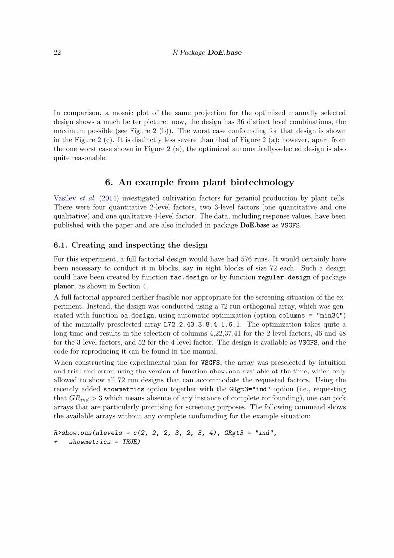
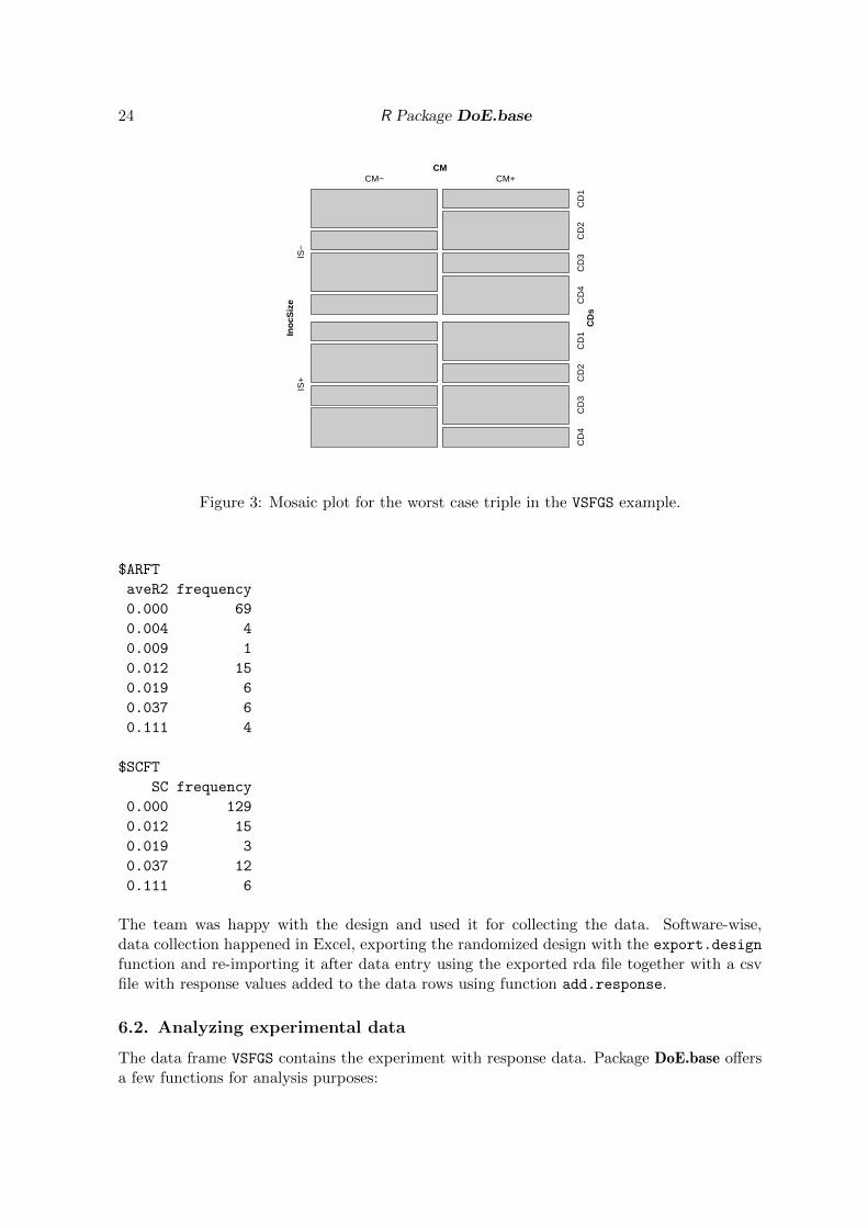
The array used in actual experimentation is the third array in this list; thus, the intuitiveapproach was successful in this case. It can be expected that all four arrays listed aboveare reasonably suited for screening the experimental factors. As the designs are far fromsaturated, optimal column allocation can substantially improve the worst case confounding:for the eventual design, the output below shows GR = GRind = 3.6, implying that the largestsquared correlation and the largest average R2 are 1/9 only; these are attained in the triples1,2,7 and 3,5,7. For illustrating the worst case degree of confounding, Figure 3 shows thetriple 3,5,7 in quite reasonable balance.
R>GRind(VSGFS)
$GRs
GR GRind
3.667 3.667
$GR.i
Light ShakFreq InocSize FilledVol CM Sugar CDs
GRtot.i 3.667 3.667 3.667 3.864 3.667 3.864 3.808
GRind.i 3.667 3.667 3.667 3.808 3.667 3.808 3.667
24 R Package DoE.base
CM
Inoc
Siz
e
CD
s
IS+
CD
4C
D3
CD
2C
D1
IS−
CM− CM+
CD
4C
D3
CD
2C
D1
Figure 3: Mosaic plot for the worst case triple in the VSFGS example.
$ARFT
aveR2 frequency
0.000 69
0.004 4
0.009 1
0.012 15
0.019 6
0.037 6
0.111 4
$SCFT
SC frequency
0.000 129
0.012 15
0.019 3
0.037 12
0.111 6
The team was happy with the design and used it for collecting the data. Software-wise,data collection happened in Excel, exporting the randomized design with the export.design
function and re-importing it after data entry using the exported rda file together with a csvfile with response values added to the data rows using function add.response.
6.2. Analyzing experimental data
The data frame VSFGS contains the experiment with response data. Package DoE.base offersa few functions for analysis purposes:
Ulrike Gromping 25
� the plot method for class design, in case of data with responses, creates simple maineffects plots, by invoking the plot method from package graphics
� the lm method for class design runs a linear model with a modifiable default degree.For orthogonal arrays created with function oa.design, the default degree is one, i.e.,a model with main effects only. Linear models can of course also be run by the lm
function from the core package stats, and analysis of variance functionality can also beused (see below).
� the halfnormal method for classes lm or design creates a half-normal effects plot (seeSection 7)
Of course, other R functionality can also be used, for example interaction plots or functionalityfor mixed model analysis. The functionality for handling repeated measurement data orreplicated data has been described for package FrF2 in Gromping (2014c, Sections 5.3 and5.9 of ) and is analogous here.
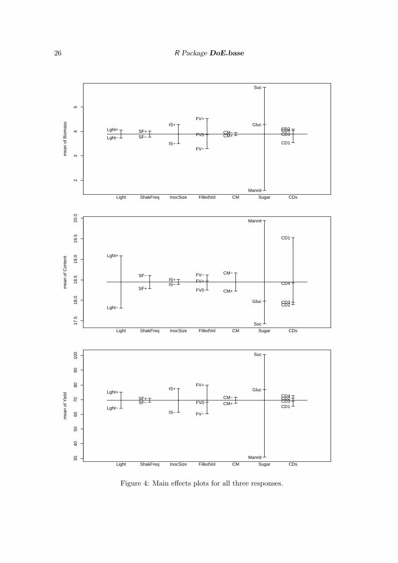
Main effects plots can be obtained by the simple command plot(VSGFS), which creates theseplots for all three response variables. Figure 4 shows the plots with default labeling, arrangedwith three plots on one page and reduced margin sizes. Of course, one would usually adaptthe annotation for final reports or publications. The plot shows that the sugar sucrose is verybeneficial for the biomass, not very good for the content, but nevertheless, because of thestrong effect on biomass, beneficial for the yield. The content apparently can be increased bychoosing the sugar mannitol, level one of factor CD and the +-level of Light. Apart from the+-level of Light, the other settings for high content are not helpful for overall yield.
An assessment of significance can be obtained from a linear model analysis. This can beobtained separately for each response, for example for the content. Here, the analysis confirmsthe findings from the main effects plot:
R>summary(lm(VSGFS, response = "Content"))
Number of observations used: 72
Formula:
Content ~ Light + ShakFreq + InocSize + FilledVol + CM + Sugar +
CDs
Call:
lm.default(formula = fo, data = model.frame(fo, data = formula))
Residuals:
Min 1Q Median 3Q Max
-2.5472 -1.1746 -0.1052 0.7008 4.6994
Coefficients:
Estimate Std. Error t value Pr(>|t|)
(Intercept) 18.67611 0.55106 33.891 < 2e-16 ***
Light1 0.63264 0.19483 3.247 0.00191 **
ShakFreq1 -0.15792 0.19483 -0.811 0.42083
26 R Package DoE.base
23
45
Factors
mea
n of
Bio
mas
s
Lght−
Lght+
SF−SF+
IS−
IS+
FV−
FV0
FV+
CM−CM+
Suc
Gluc
Mannit
CD1
CD2CD3CD4
Light ShakFreq InocSize FilledVol CM Sugar CDs
17.5
18.0
18.5
19.0
19.5
20.0
Factors
mea
n of
Con
tent
Lght−
Lght+
SF−
SF+IS−IS+
FV−
FV0
FV+
CM−
CM+
Suc
Gluc
Mannit
CD1
CD2CD3
CD4
Light ShakFreq InocSize FilledVol CM Sugar CDs
3040
5060
7080
9010
0
mea
n of
Yie
ld
Lght−
Lght+
SF−SF+
IS−
IS+
FV−
FV0
FV+
CM−CM+
Suc
Gluc
Mannit
CD1
CD2CD3CD4
Light ShakFreq InocSize FilledVol CM Sugar CDs
Figure 4: Main effects plots for all three responses.

Ulrike Gromping 27
InocSize1 0.05903 0.19483 0.303 0.76296
FilledVolFV0 -0.36958 0.47723 -0.774 0.44172
FilledVolFV+ -0.14958 0.47723 -0.313 0.75503
CM1 -0.22069 0.19483 -1.133 0.26182
SugarGluc 0.54917 0.47723 1.151 0.25441
SugarMannit 2.51167 0.47723 5.263 2e-06 ***
CDsCD2 -1.63222 0.55106 -2.962 0.00438 **
CDsCD3 -1.57111 0.55106 -2.851 0.00597 **
CDsCD4 -1.10722 0.55106 -2.009 0.04901 *
---
Signif. codes: 0 '***' 0.001 '**' 0.01 '*' 0.05 '.' 0.1 ' ' 1
Residual standard error: 1.653 on 60 degrees of freedom
Multiple R-squared: 0.4787, Adjusted R-squared: 0.3831
F-statistic: 5.008 on 11 and 60 DF, p-value: 1.75e-05
The model explains less than 50% of the response variability, which is far from perfect. Thestrong heredity principle – interactions are only active if both their component factors areactive – suggests to look at a model with the three active main effect factors and theirinteractions, which leaves a somewhat confusing picture (not shown).
For the data at hand, there are enough degrees of freedom to run an Anova analysis withthe full degree 2 model. Of course, while main effects are orthogonal to each other, 2-factorinteractions can be slightly confounded with main effects and severely confounded with other2-factor interactions. However, at least, the theory tells us that the estimable effects canbe estimated without bias (unless effects of order higher than two bias them). As Anovaanalyses sums of squares, the analysis is invariant with respect to factor coding. In orderto obtain an order-invariant assessment of significance, the function Anova from package car(Fox and Weisberg 2011) can be used; contrary to function anova from package stats, Anovaavoids order-dependence by using type II sums of squares, which condition on all other effectsexcept for ones that contain the effect under investigation. The results point to the maineffects that were also identified before, and a liberal look at p values additionally indicatessome marginal 2-factor interactions (Sugar with each of InocSize, FilledVol, CDs, Light,and ShakFreq:CM, which is completely unrelated to the active main effects).
R>require("car")
R>Anova(lm(VSGFS, response = "Content", degree = 2))
Anova Table (Type II tests)
Response: Content
Sum Sq Df F value Pr(>F)
Light 16.345 1 8.2606 0.0165515 *
ShakFreq 0.483 1 0.2441 0.6319195
InocSize 1.604 1 0.8105 0.3891387
FilledVol 0.889 2 0.2247 0.8026463
CM 0.805 1 0.4069 0.5378565
28 R Package DoE.base
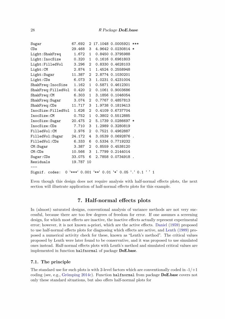
Sugar 67.692 2 17.1048 0.0005921 ***
CDs 29.468 3 4.9642 0.0230814 *
Light:ShakFreq 1.672 1 0.8450 0.3795988
Light:InocSize 0.320 1 0.1616 0.6961803
Light:FilledVol 3.296 2 0.8330 0.4628103
Light:CM 2.874 1 1.4524 0.2558948
Light:Sugar 11.387 2 2.8774 0.1030201
Light:CDs 6.073 3 1.0231 0.4231004
ShakFreq:InocSize 1.162 1 0.5871 0.4612301
ShakFreq:FilledVol 0.420 2 0.1061 0.9003686
ShakFreq:CM 6.303 1 3.1856 0.1046054
ShakFreq:Sugar 3.074 2 0.7767 0.4857813
ShakFreq:CDs 11.717 3 1.9738 0.1819413
InocSize:FilledVol 1.626 2 0.4109 0.6737704
InocSize:CM 0.752 1 0.3802 0.5512885
InocSize:Sugar 20.475 2 5.1739 0.0286697 *
InocSize:CDs 7.710 3 1.2989 0.3280819
FilledVol:CM 2.976 2 0.7521 0.4962887
FilledVol:Sugar 24.172 4 3.0539 0.0692876 .
FilledVol:CDs 6.333 6 0.5334 0.7719232
CM:Sugar 3.387 2 0.8559 0.4538120
CM:CDs 10.566 3 1.7799 0.2144014
Sugar:CDs 33.075 6 2.7858 0.0734918 .
Residuals 19.787 10
---
Signif. codes: 0 '***' 0.001 '**' 0.01 '*' 0.05 '.' 0.1 ' ' 1
Even though this design does not require analysis with half-normal effects plots, the nextsection will illustrate application of half-normal effects plots for this example.
7. Half-normal effects plots
In (almost) saturated designs, conventional analysis of variance methods are not very suc-cessful, because there are too few degrees of freedom for error. If one assumes a screeningdesign, for which most effects are inactive, the inactive effects actually represent experimentalerror; however, it is not known a-priori, which are the active effects. Daniel (1959) proposedto use half-normal effects plots for diagnosing which effects are active, and Lenth (1989) pro-posed a numerical activity check for these, known as “Lenth’s method”. The critical valuesproposed by Lenth were later found to be conservative, and it was proposed to use simulatedones instead. Half-normal effects plots with Lenth’s method and simulated critical values areimplemented in function halfnormal of package DoE.base.
7.1. The principle
The standard use for such plots is with 2-level factors which are conventionally coded in -1/+1coding (see, e.g., Gromping 2014c). Function halfnormal from package DoE.base covers notonly these standard situations, but also offers half-normal plots for
Ulrike Gromping 29
� 2-level designs with a few error degrees of freedom. For these, it automatically augmentsthe estimated effects with error effects, distinguishing these into lack-of-fit and pureerror. Significance assessment can be done with Lenth’s method on the augmented setof estimates, or with other methods proposed in the literature (Larntz and Whitcomb1998; Edwards and Mee 2008). Note that error effects are not necessarily uniquelydetermined.
� 2-level designs with partially confounded effects. For these, it projects out all precedingeffects from the remaining ones (thus, the plotting points depend on the model orderfor such situations).
� mixed level designs, for which there is no unique coding and the plotting points arecoding dependent. Mixed level designs can also have error degrees of freedom or partiallyconfounded effects.
The strategy chosen in function halfnormal seems to be similar to that applied in the JMPsoftware screening platform (see Chapter 8 of SAS Institute, Inc. 2012), both regarding thetreatment of error points and the single degree of freedom representations for factors withmore than two levels. On the contrary, Design-Expert (Stat-Ease Inc. 2012) does not plotindividual degrees of freedom, but scaled Chi-squared values for effects with more than onedegree of freedom. This avoids the coding dependence, but has the adverse effect that thenumber of plotting points is small so that effect sparsity is not easily achieved.
The steps for augmenting the estimated effects with error degrees of freedom are described,e.g., in Gromping (2015a) and are very similar also to the suggestions by Langsrud (2001) ina different context. A coarse overview works as follows:
� Make sure the model matrix X has orthogonal columns all of which have the sameEuclidean length; if this is not the case, X has to be pre-treated (see below).
� For N observations, a trivial saturated model matrix is the N -dimensional identitymatrix IN . If a distinction between lack-of-fit and pure error is sought, one can replacethis matrix by a matrix S of dummy variables for distinct runs, and additionally includeappropriately scaled orthogonal contrast matrices for replicated runs. In the following,for simplicity, IN is used.
� Residualize the matrix IN by projecting out the model matrix X, i.e., calculate theresidual matrix R = IN −X(X>X)−1X>.
� Create the half-normal effects plot for the augmented model matrix (X|R), which hasbeen created such that it has orthogonal columns of all the same length.
The pre-treatment mentioned in the first bullet is as follows: If X has orthogonal columnsof varying Euclidean lengths, one simply has to normalize all columns to a common length.The case of non-orthogonal columns is more demanding and will be discussed using the modelmatrix X for a full model in an unreplicated full factorial for one 2-level and one 3-level factor,
30 R Package DoE.base
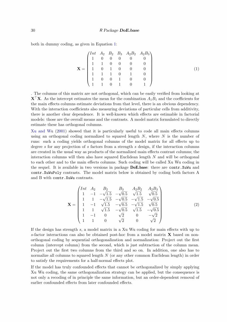
both in dummy coding, as given in Equation 1:
X =
Int A2 B2 B3 A2B2 A2B3
1 0 0 0 0 01 1 0 0 0 01 0 1 0 0 01 1 1 0 1 01 0 0 1 0 01 1 0 1 0 1
(1)
. The columns of this matrix are not orthogonal, which can be easily verified from looking atX>X. As the intercept estimates the mean for the combination A1B1 and the coefficients forthe main effects columns estimate deviations from that level, there is an obvious dependency.With the interaction coefficients also measuring deviations of particular cells from additivity,there is another clear dependence. It is well-known which effects are estimable in factorialmodels: those are the overall means and the contrasts. A model matrix formulated to directlyestimate these has orthogonal columns.
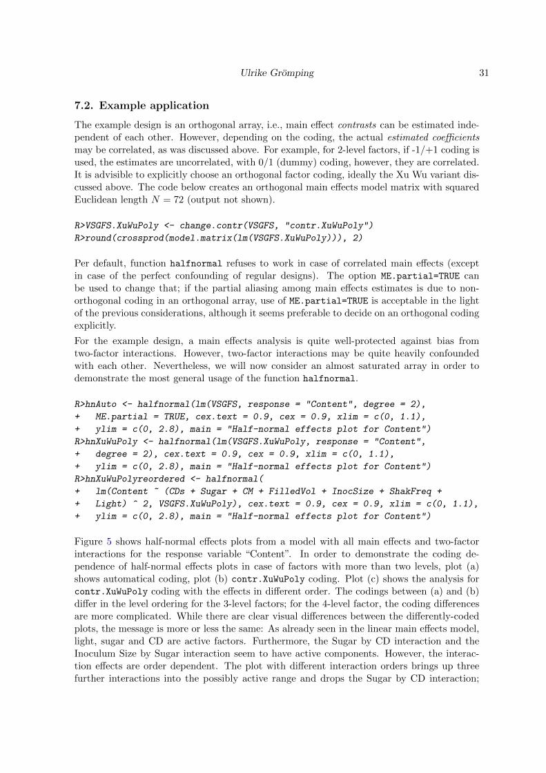
Xu and Wu (2001) showed that it is particularly useful to code all main effects columnsusing an orthogonal coding normalized to squared length N , where N is the number ofruns: such a coding yields orthogonal columns of the model matrix for all effects up todegree s for any projection of s factors from a strength s design, if the interaction columnsare created in the usual way as products of the normalized main effects contrast columns; theinteraction columns will then also have squared Euclidean length N and will be orthogonalto each other and to the main effects columns. Such coding will be called Xu Wu coding inthe sequel. It is available in two versions in package DoE.base: there are contr.XuWu andcontr.XuWuPoly contrasts. The model matrix below is obtained by coding both factors Aand B with contr.XuWu contrasts.
X =
Int A2 B2 B3 A2B2 A2B3
1 −1 −√
1.5 −√
0.5√
1.5√
0.5
1 1 −√
1.5 −√
0.5 −√
1.5 −√
0.5
1 −1√
1.5 −√
0.5 −√
1.5√
0.5
1 1√
1.5 −√
0.5√
1.5 −√
0.5
1 −1 0√
2 0 −√
2
1 1 0√
2 0√
2
(2)
If the design has strength s, a model matrix in a Xu Wu coding for main effects with up tos-factor interactions can also be obtained post-hoc from a model matrix X based on non-orthogonal coding by sequential orthogonalization and normalization: Project out the firstcolumn (intercept column) from the second, which is just subtraction of the column mean.Project out the first two columns from the third and so on. In addition, one also has tonormalize all columns to squared length N (or any other common Euclidean length) in orderto satisfy the requirements for a half-normal effects plot.
If the model has truly confounded effects that cannot be orthogonalized by simply applyingXu Wu coding, the same orthogonalization strategy can be applied, but the consequence isnot only a recoding of in principle the same information, but an order-dependent removal ofearlier confounded effects from later confounded effects.
Ulrike Gromping 31
7.2. Example application
The example design is an orthogonal array, i.e., main effect contrasts can be estimated inde-pendent of each other. However, depending on the coding, the actual estimated coefficientsmay be correlated, as was discussed above. For example, for 2-level factors, if -1/+1 coding isused, the estimates are uncorrelated, with 0/1 (dummy) coding, however, they are correlated.It is advisible to explicitly choose an orthogonal factor coding, ideally the Xu Wu variant dis-cussed above. The code below creates an orthogonal main effects model matrix with squaredEuclidean length N = 72 (output not shown).
R>VSGFS.XuWuPoly <- change.contr(VSGFS, "contr.XuWuPoly")
R>round(crossprod(model.matrix(lm(VSGFS.XuWuPoly))), 2)
Per default, function halfnormal refuses to work in case of correlated main effects (exceptin case of the perfect confounding of regular designs). The option ME.partial=TRUE canbe used to change that; if the partial aliasing among main effects estimates is due to non-orthogonal coding in an orthogonal array, use of ME.partial=TRUE is acceptable in the lightof the previous considerations, although it seems preferable to decide on an orthogonal codingexplicitly.
For the example design, a main effects analysis is quite well-protected against bias fromtwo-factor interactions. However, two-factor interactions may be quite heavily confoundedwith each other. Nevertheless, we will now consider an almost saturated array in order todemonstrate the most general usage of the function halfnormal.
R>hnAuto <- halfnormal(lm(VSGFS, response = "Content", degree = 2),
+ ME.partial = TRUE, cex.text = 0.9, cex = 0.9, xlim = c(0, 1.1),
+ ylim = c(0, 2.8), main = "Half-normal effects plot for Content")
R>hnXuWuPoly <- halfnormal(lm(VSGFS.XuWuPoly, response = "Content",
+ degree = 2), cex.text = 0.9, cex = 0.9, xlim = c(0, 1.1),
+ ylim = c(0, 2.8), main = "Half-normal effects plot for Content")
R>hnXuWuPolyreordered <- halfnormal(
+ lm(Content ~ (CDs + Sugar + CM + FilledVol + InocSize + ShakFreq +
+ Light) ^ 2, VSGFS.XuWuPoly), cex.text = 0.9, cex = 0.9, xlim = c(0, 1.1),
+ ylim = c(0, 2.8), main = "Half-normal effects plot for Content")
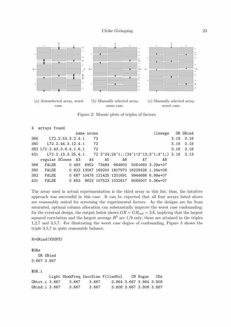
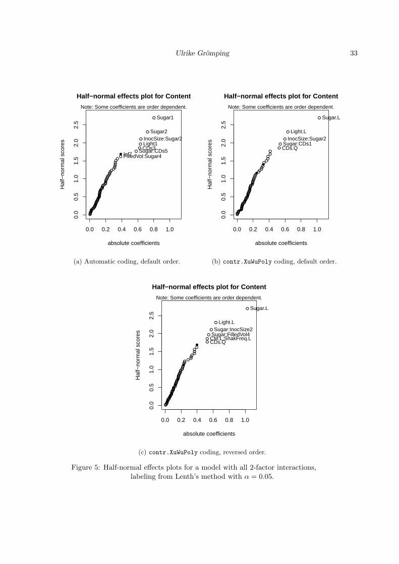
Figure 5 shows half-normal effects plots from a model with all main effects and two-factorinteractions for the response variable “Content”. In order to demonstrate the coding de-pendence of half-normal effects plots in case of factors with more than two levels, plot (a)shows automatical coding, plot (b) contr.XuWuPoly coding. Plot (c) shows the analysis forcontr.XuWuPoly coding with the effects in different order. The codings between (a) and (b)differ in the level ordering for the 3-level factors; for the 4-level factor, the coding differencesare more complicated. While there are clear visual differences between the differently-codedplots, the message is more or less the same: As already seen in the linear main effects model,light, sugar and CD are active factors. Furthermore, the Sugar by CD interaction and theInoculum Size by Sugar interaction seem to have active components. However, the interac-tion effects are order dependent. The plot with different interaction orders brings up threefurther interactions into the possibly active range and drops the Sugar by CD interaction;
32 R Package DoE.base
thus, clearly, one has to be cautious with statements on these effects from half-normal effectsplots. However, all effects that show up in the half-normal effects plots have also been at leastmarginal in the Anova analysis of the previous section.
The calculation results have been stored in the list objects
hnAuto, hnXuWuPoly, and hnXuWuPolyreordered,
respectively. The list element res simply indicates which effects have been projected out fromwhich other effects; furthermore, the results contain the model matrix after orthogonalization,and details about the orthogonalization itself. Printed output of orthogonalization steps hasbeen suppressed here. The reader is encouraged to check the printed output of the simplecommand
R>hnAuto <- halfnormal(VSGFS, ME.partial = TRUE, plot = FALSE)
which explains how columns of the main effects model matrix stored in
R>mm <- hnAuto$mm[, 2:11]
are obtained from the original model matrix stored (without intercept column) in
R>desnum(VSGFS)[, 1:10]
8. Further developments
Package DoE.base tries a balancing act of offering tools both for practitioners with a relativelyweak statistical background and for statistical experts. In order to save the former fromavoidable grave mistakes, the package takes a cautious strategy issuing many warnings, wheredesigns might be improvable or analyses might be inadequate. In various cases, it would bedesirable to avoid unnecessary warnings; for example, there are arrays for which it is knownfrom theoretical work (Butler 2005) that all choices for certain columns are GMA. For thesearrays, warnings for array optimization should be eliminated, which requires some slightlytedious work.
The current design catalog covers many situations, but is also limited especially with respectto availability of non-regular designs. Augmenting the catalog with further useful non-regulardesigns is a difficult task and should not be addressed before studying in more detail therelation between recently developed design quality criteria like GR, GRind, ARFT and SCFTand a design’s usefulness for experimentation.
So far, the design catalog is used for selecting designs and optimizing column choices fromthem. Kuhfeld (2010) makes much more extensive use of the catalog within a SAS software
Ulrike Gromping 33
●●●●●●●●●
●●●●●●●●●●●●●●●●●●●●●●●●●●●●●●●●●●
●●●●●●●●●●●●●●●
●●●●●
●●
●●
●
●
●
●
0.0 0.2 0.4 0.6 0.8 1.0
0.0
0.5
1.0
1.5
2.0
2.5
Half−normal effects plot for Content
absolute coefficients
Hal
f−no
rmal
sco
res
FilledVol:Sugar4 lof7 Sugar:CDs5 CDs3
Light1 InocSize:Sugar2
Sugar2
Sugar1
Note: Some coefficients are order dependent.
(a) Automatic coding, default order.
●●●●●●●●●●
●●●●●●●●●●●●●●●●●●●●●●●●●●●●●●●●●●●●●●●●●●●●
●●●●●●●
●●●
●●
●
●
●
●
●
0.0 0.2 0.4 0.6 0.8 1.00.
00.
51.
01.
52.
02.
5
Half−normal effects plot for Content
absolute coefficients
Hal
f−no
rmal
sco
res
CDs.Q Sugar:CDs1
InocSize:Sugar2 Light.L
Sugar.L
Note: Some coefficients are order dependent.
(b) contr.XuWuPoly coding, default order.
●●●●●●●●●●●●●●●●●●●●●●●●●●●●●●●●●●●●●●●●●●●●●●●●●●
●●●●●●
●●●●
●●●
●●
●●
●
●
●
●
0.0 0.2 0.4 0.6 0.8 1.0
0.0
0.5
1.0
1.5
2.0
2.5
Half−normal effects plot for Content
absolute coefficients
Hal
f−no
rmal
sco
res
CDs.Q CM.L:ShakFreq.L Sugar:FilledVol4 Sugar:InocSize2
Light.L
Sugar.L
Note: Some coefficients are order dependent.
(c) contr.XuWuPoly coding, reversed order.
Figure 5: Half-normal effects plots for a model with all 2-factor interactions,labeling from Lenth’s method with α = 0.05.
34 R Package DoE.base
macro suite for creating experimental designs from the arrays in the catalog, specificallycreated with marketing applications in mind (Kuhfeld 2010). Such use can certainly also becombined with the catalog in package DoE.base. The dependent package support.CEs (Aizaki2012) implements choice experiments in R. However, implementing a functionality as flexibleas the one offered in the (Kuhfeld 2010) SAS macros would require substantial additionaleffort.
Package DoE.base also serves as a tool for supporting further theoretical investigations intoaspects like design regularity and new design quality criteria.
Last but not least, the class design and infrastructure for it are also available for use byother packages. Authors of other S3-based packages are invited to use it; the methods withinpackage DoE.base for its class design can be adjusted to accommodate further types of design;please inform the package maintainer, if you would like a new type of design included intothe methods offered.
Acknowledgments
Boyko Amarov and Hongquan Xu contributed code to the package. Creation of generalizedresolution functionality was partly supported by grant GR 3843/1-1 of Deutsche Forschungs-gemeinschaft.
References
Aizaki H (2012). “Basic Functions for Supporting an Implementation of Choice Experimentsin R.” Journal of Statistical Software, Code Snippets, 50(2), 1–24. ISSN 1548-7660. URLhttp://www.jstatsoft.org/v50/c02.
Box G, Tyssedal J (1996). “Projective Properties of Certain Orthogonal Arrays.” Biometrika,83, 950–955.
Butler N (2005). “Generalised Minimum Aberration Construction Results for SymmetricalOrthogonal Arrays.” Biometrika, 92, 485–491.
Chambers J, Hastie T (1984). Statistical Models in S. Wadsworth & Brooks/Cole, PacificGrove, CA.
Chasalow S (2012). combinat: Combinatorics Utilities. R package version 0.0-8, URLhttp://CRAN.R-project.org/package=combinat.
Collings B (1984). “Generating the Intrablock and Interblock Subgroups for Confounding inGeneral Factorial Experiments.” The Annals of Statistics, 12, 1500–1509.
Collings B (1989). “Quick Confounding.” Technometrics, 31, 107–110.
Daniel C (1959). “Use of Half Normal Plots in Interpreting Two Level Experiments.” Tech-nometrics, 1, 311–340.
Deng LY, Tang B (1999). “Generalized Resolution and Minimum Aberration Criteria forPlackett-Burman and Other Nonregular Factorial Designs.” Statistica Sinica, 9, 1072–1082.
Ulrike Gromping 35
Edwards D, Mee R (2008). “Empirically Determined p-Values for Lenth t-Statistics.” Journalof Quality Technology, 40, 368–380.
Eendebak P, Schoen E (2010). “Complete Series of Non-Isomorphic Orthogonal Arrays.” URLhttp://pietereendebak.nl/oapage/.
Fox J, Weisberg S (2011). An R Companion to Applied Regression. 2nd edition. Sage, Thou-sand Oaks CA. URL http://socserv.socsci.mcmaster.ca/jfox/Books/Companion.
Gromping U (2011a). “Relative Projection Frequency Tables for Orthogonal Arrays.” Reportsin Mathematics, Physics and Chemistry 1, Beuth University of Applied Sciences Berlin,Germany.
Gromping U (2011b). “Tutorial for Designing Experiments Using the R Package RcmdrPlu-gin.DoE.” Reports in Mathematics, Physics and Chemistry 4, Beuth University of AppliedSciences Berlin, Germany.
Gromping U (2013a). “Frequency Tables for the Coding Invariant Ranking of OrthogonalArrays.” Reports in Mathematics, Physics and Chemistry 2, Beuth University of AppliedSciences Berlin, Germany.
Gromping U (2013b). DoE.wrapper: Wrapper Package for Design of Experiments Function-ality. R package version 0.8-9, URL http://CRAN.R-project.org/package=DoE.wrapper.
Gromping U (2013c). FrF2.catlg128: Complete Catalogues of Resolution IV 128 Run 2-Level Fractional Factorials up to 24 Factors. R package version 1.2-1, URL http://CRAN.
R-project.org/package=FrF2.
Gromping U (2013d). RcmdrPlugin.DoE: R Commander Plugin for (Industrial) Designof Experiments. R package version 0.12-2, URL http://CRAN.R-project.org/package=
RcmdrPlugin.DoE.
Gromping U (2014a). “Mosaic Plots Are Useful for Visualizing Low Order Projections ofFactorial Designs.” The American Statistician, 68(2), 108–116.
Gromping U (2014b). FrF2: Fractional Factorial Designs With 2-Level Factors. R packageversion 1.7-1, URL http://CRAN.R-project.org/package=FrF2.
Gromping U (2014c). “R Package FrF2 for Creating and Analyzing Fractional Factorial2-Level Designs.” Journal of Statistical Software, 56(1), 1–56. ISSN 1548-7660. URLhttp://www.jstatsoft.org/v56/i01.
Gromping U (2015a). “Augmented Half Normal Effects Plots in the Presence of a Few ErrorDegrees of Freedom.” Quality and Reliability International, 31(7), 1185–1196.
Gromping U (2015b). DoE.base: Full Factorials, Orthogonal Arrays and Base Utilities forDoE Packages. R package version 0.27-1, URL http://CRAN.R-project.org/package=
DoE.base.
Gromping U, Xu H (2014). “Generalized Resolution for Orthogonal Arrays.” The Annals ofStatistics, 42(3), 918–939.
36 R Package DoE.base
Kobilinsky A, Bouvier A, Monod H (2015a). planor: Generation of Regular Factorial De-signs. R package version 0.2-3, URL http://CRAN.R-project.org/package=planor.
Kobilinsky A, Monod H, Bailey R (2015b). “Automatic Generation of Generalised RegularFactorial Designs.” Preprint Series 7, Issac Newton Institue for Mathematical Sciences,London, UK.
Kuhfeld W (2010). “Orthogonal Arrays.” URL http://support.sas.com/techsup/
technote/ts723.html.
Langsrud O (2001). “Identifying Significant Effects in Fractional Factorial MultiresponseExperiments.” Technometrics, 43, 415–424.
Larntz K, Whitcomb P (1998). “Use of Replication in Almost Unreplicated Factorials.”Manuscript of a presentation given at the 42nd ASQ Fall Technical conference in Corn-ing, New York, downloaded April 26, 2013., URL http://www.statease.com/pubs/
use-of-rep.pdf.
Lenth R (1989). “Quick and Easy Analysis of Unreplicated Factorials.” Technometrics, 31,469–473.
Meyer D, Zeileis A, Hornik K (2013). vcd: Visualizing Categorical Data. R package version 1.3-1, URL http://CRAN.R-project.org/package=vcd.
NIST/SEMATECH (2012). “NIST/SEMATECH e-Handbook of Statistical Methods, Sec-tion 3.” Accessed 17 Feb 2015, URL http://www.itl.nist.gov/div898/handbook/pri/
section3/pri33a.htm.
Plackett R, Burman J (1946). “The Design of Optimum Multifactorial Experiments.”Biometrika, 33(4), 305–325. doi:10.1093/biomet/33.4.305.
R Development Core Team (2015). R: A Language and Environment for Statistical Computing.R Foundation for Statistical Computing, Vienna, Austria. URL http://www.R-project.
org.
SAS Institute, Inc (2012). JMP Modeling and Multivariate Methods. Cary,NC. Chapter 8, URL https://www.jmp.com/support/downloads/pdf/jmp1002/
Modeling-and-Multivariate-Methods.pdf.
Schoen E, Eendebak P, Nguyen M (2010). “Complete Enumeration of Pure-Level and Mixed-Level Orthogonal Arrays.” Journal of Combinatorial Designs, 18(2), 123–140.
Stat-Ease Inc (2012). Design-Expert, Version 8.
Tang B, Deng LY (1999). “Minimum G2-Aberration for Nonregular Fractional FactorialDesigns.” The Annals of Statistics, 27, 1914–1926.
Vasilev N, Schmitz C, Gromping U, Fischer R, Schillberg S (2014). “Assessment of Culti-vation Factors that Affect Biomass and Geraniol Production in Transgenic Tobacco CellSuspension Cultures.” PLOS one, 9(8), 1–7. doi:10.1371/journal.pone.0104620.
Venables B (2013). conf.design: Construction of Factorial Designs. R package version 2.0.0,URL http://CRAN.R-project.org/package=conf.design.
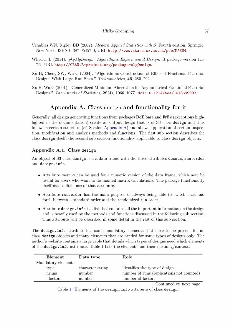
Ulrike Gromping 37
Venables WN, Ripley BD (2002). Modern Applied Statistics with S. Fourth edition. Springer,New York. ISBN 0-387-95457-0, URL http://www.stats.ox.ac.uk/pub/MASS4.
Wheeler B (2014). pkgAlgDesign: Algorithmic Experimental Design. R package version 1.1-7.2, URL http://CRAN.R-project.org/package=AlgDesign.
Xu H, Cheng SW, Wu C (2004). “Algorithmic Construction of Efficient Fractional FactorialDesigns With Large Run Sizes.” Technometrics, 46, 280–292.
Xu H, Wu C (2001). “Generalized Minimum Aberration for Asymmetrical Fractional FactorialDesigns.” The Annals of Statistics, 29(4), 1066–1077. doi:10.1214/aos/1013699993.
Appendix A. Class design and functionality for it
Generally, all design generating functions from packages DoE.base and FrF2 (exceptions high-lighted in the documentation) create an output design that is of S3 class design and thusfollows a certain structure (cf. Section Appendix A) and allows application of certain inspec-tion, modification and analysis methods and functions. The first sub section describes theclass design itself, the second sub section functionality applicable to class design objects.
Appendix A.1. Class design
An object of S3 class design is a a data frame with the three attributes desnum, run.orderand design.info.
� Attribute desnum can be used for a numeric version of the data frame, which may beuseful for users who want to do manual matrix calculations. The package functionalityitself makes little use of that attribute.
� Attribute run.order has the main purpose of always being able to switch back andforth between a standard order and the randomized run order.
� Attribute design.info is a list that contains all the important information on the designand is heavily used by the methods and functions discussed in the following sub section.This attribute will be described in some detail in the rest of this sub section.
The design.info attribute has some mandatory elements that have to be present for allclass design objects and many elements that are needed for some types of designs only. Theauthor’s website contains a large table that details which types of designs need which elementsof the design.info attribute. Table 1 lists the elements and their meaning/context.
Element Data type Role
Mandatory elementstype character string identifies the type of designnruns number number of runs (replications not counted)nfactors number number of factors
Continued on next pageTable 1: Elements of the design.info attribute of class design.
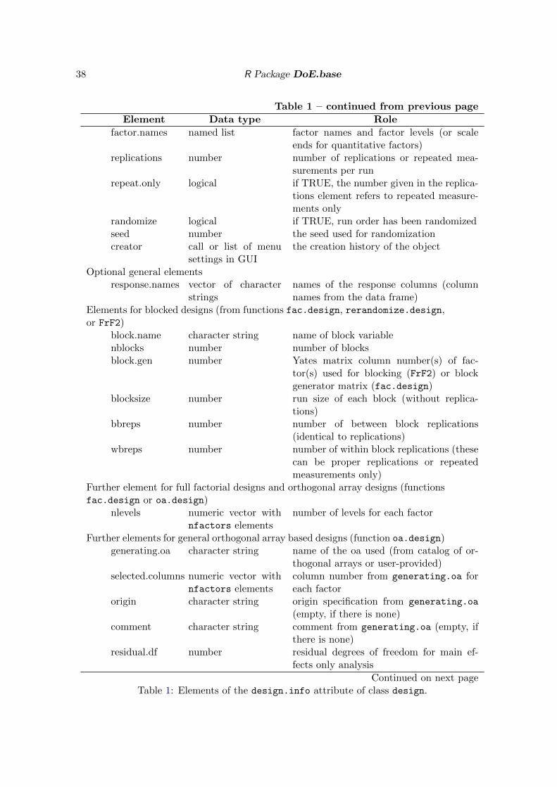
38 R Package DoE.base
Table 1 – continued from previous page
Element Data type Role
factor.names named list factor names and factor levels (or scaleends for quantitative factors)
replications number number of replications or repeated mea-surements per run
repeat.only logical if TRUE, the number given in the replica-tions element refers to repeated measure-ments only
randomize logical if TRUE, run order has been randomizedseed number the seed used for randomizationcreator call or list of menu
settings in GUIthe creation history of the object
Optional general elementsresponse.names vector of character
stringsnames of the response columns (columnnames from the data frame)
Elements for blocked designs (from functions fac.design, rerandomize.design,or FrF2)
block.name character string name of block variablenblocks number number of blocksblock.gen number Yates matrix column number(s) of fac-
tor(s) used for blocking (FrF2) or blockgenerator matrix (fac.design)
blocksize number run size of each block (without replica-tions)
bbreps number number of between block replications(identical to replications)
wbreps number number of within block replications (thesecan be proper replications or repeatedmeasurements only)
Further element for full factorial designs and orthogonal array designs (functionsfac.design or oa.design)
nlevels numeric vector withnfactors elements
number of levels for each factor
Further elements for general orthogonal array based designs (function oa.design)generating.oa character string name of the oa used (from catalog of or-
thogonal arrays or user-provided)selected.columns numeric vector with
nfactors elementscolumn number from generating.oa foreach factor
origin character string origin specification from generating.oa
(empty, if there is none)comment character string comment from generating.oa (empty, if
there is none)residual.df number residual degrees of freedom for main ef-
fects only analysis
Continued on next pageTable 1: Elements of the design.info attribute of class design.
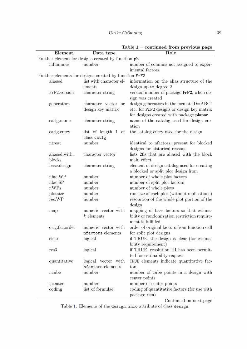
Ulrike Gromping 39
Table 1 – continued from previous page
Element Data type Role
Further element for designs created by function pb
ndummies number number of columns not assigned to exper-imental factors
Further elements for designs created by function FrF2
aliased list with character el-ements
information on the alias structure of thedesign up to degree 2
FrF2.version character string version number of package FrF2, when de-sign was created
generators character vector ordesign key matrix
design generators in the format “D=ABC”etc. for FrF2 designs or design key matrixfor designs created with package planor
catlg.name character string name of the catalog used for design cre-ation
catlg.entry list of length 1 ofclass catlg
the catalog entry used for the design
ntreat number identical to nfactors, present for blockeddesigns for historical reasons
aliased.with.blocks
character vector lists 2fis that are aliased with the blockmain effect
base.design character string element of design catalog used for creatinga blocked or split plot design from
nfac.WP number number of whole plot factorsnfac.SP number number of split plot factorsnWPs number number of whole plotsplotsize number run size of each plot (without replications)res.WP number resolution of the whole plot portion of the
designmap numeric vector with
k elementsmapping of base factors so that estima-bility or randomization restriction require-ment is fulfilled
orig.fac.order numeric vector withnfactors elements
order of original factors from function callfor split plot designs
clear logical if TRUE, the design is clear (for estima-bility requirement)
res3 logical if TRUE, resolution III has been permit-ted for estimability request
quantitative logical vector withnfactors elements
TRUE elements indicate quantitative fac-tors
ncube number number of cube points in a design withcenter points
ncenter number number of center pointscoding list of formulae coding of quantitative factors (for use with
package rsm)
Continued on next pageTable 1: Elements of the design.info attribute of class design.
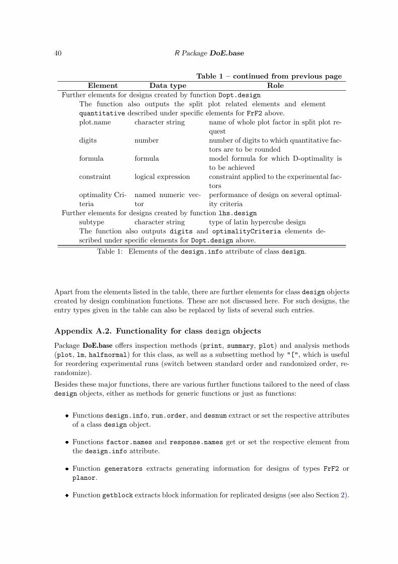
40 R Package DoE.base
Table 1 – continued from previous page
Element Data type Role
Further elements for designs created by function Dopt.design
The function also outputs the split plot related elements and elementquantitative described under specific elements for FrF2 above.plot.name character string name of whole plot factor in split plot re-
questdigits number number of digits to which quantitative fac-
tors are to be roundedformula formula model formula for which D-optimality is
to be achievedconstraint logical expression constraint applied to the experimental fac-
torsoptimality Cri-teria
named numeric vec-tor
performance of design on several optimal-ity criteria
Further elements for designs created by function lhs.design
subtype character string type of latin hypercube designThe function also outputs digits and optimalityCriteria elements de-scribed under specific elements for Dopt.design above.
Table 1: Elements of the design.info attribute of class design.
Apart from the elements listed in the table, there are further elements for class design objectscreated by design combination functions. These are not discussed here. For such designs, theentry types given in the table can also be replaced by lists of several such entries.
Appendix A.2. Functionality for class design objects
Package DoE.base offers inspection methods (print, summary, plot) and analysis methods(plot, lm, halfnormal) for this class, as well as a subsetting method by "[", which is usefulfor reordering experimental runs (switch between standard order and randomized order, re-randomize).
Besides these major functions, there are various further functions tailored to the need of classdesign objects, either as methods for generic functions or just as functions:
� Functions design.info, run.order, and desnum extract or set the respective attributesof a class design object.
� Functions factor.names and response.names get or set the respective element fromthe design.info attribute.
� Function generators extracts generating information for designs of types FrF2 orplanor.
� Function getblock extracts block information for replicated designs (see also Section 2).

Ulrike Gromping 41
� Function rerandomize.design allows to re-randomize a class design object with-out response data; this also allows explicit blocking of designs created with functionsoa.design and pb (see also Section 5.3).
� Functions for designs that can be both in wide or in long format, i.e., parameter designsand designs with repeated measurements, can change between long and wide formator aggregate wide format designs: function rep2wide brings repeated measurement de-signs into wide format, reptolong does the opposite; function paramtowide brings aparameter design to wide format (irreversible, they are created in long format); func-tion aggregate.design (method for the generic aggregate) aggregates designs in wideformat into designs with a single response.
� Functions add.response and col.remove add responses or remove columns; functionresponse.names can also be used to remove response columns.
� Function qua.design influences, which design columns are quantitative,function change.contr changes the contrasts of design columns.
� Functions undesign and redesign remove the class design properties from an objector reinstate them.
� Functions cross.design and param.design combine class design objects into crosseddesigns or parameter designs, respectively.
� Function fix.design is a method for the generic fix and has been adapted from packageutils; it allows to edit design objects; however, its use is not recommended.
� Function export.design can export a design in html or csv format, together with anR workspace for the design. After entering response data in a spreadsheet program,responses can be added to the design itself using the add.response function.
Affiliation:
Ulrike GrompingDepartment II – Mathematics, Physics, ChemistryBeuth University of Applied Sciences BerlinD-13353 BerlinE-mail: [email protected]: http://prof.beuth-hochschule.de/groemping/