Embed Size (px)
Citation preview

3/28/2011 1
Face Recognition:
Long-Range and Surveillance
Walter Scheirer
Archana Sapkota
University of Colorado at Colorado Springs and Securics, Inc.
(http://www.cs.uccs.edu/~asapkota/fg11/)
3/28/2011 2
In this tutorial, you will learn about:
1. Motivating Concerns over Surveillance with Biometrics in Difficult Environments
2. Lighting Considerations
3. Optics Considerations
4. Sensor Considerations
5. Weather and Atmospheric Impacts
6. Data Sets for Evaluations
7. Controlled Experiments for Large Scale Collections
8. Challenges for Image Quality Assessment
9. Advanced Feature Detection
10. Mitigating the Effect of Blur
3/28/2011 3
In this tutorial, you will learn about:
11. Features for Recognition
12. 3D Approaches
13. Video Based Approaches
14. Pose & Occlusion Invariance
15. Biologically Inspired Methods
16. Image Quality
17. Meta-Recognition for Post Recognition Score
Analysis

3/28/2011 4
Motivating Concerns
3/28/2011 5
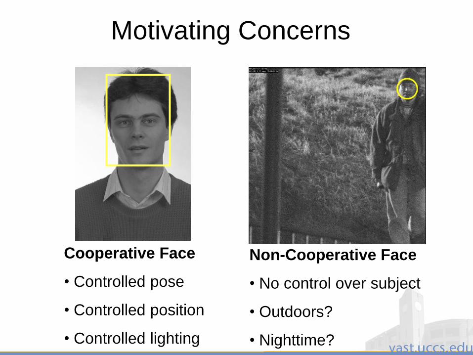
Motivating Concerns
Cooperative Face
• Controlled pose
• Controlled position
• Controlled lighting
Non-Cooperative Face
• No control over subject
• Outdoors?
• Nighttime?
3/28/2011 6
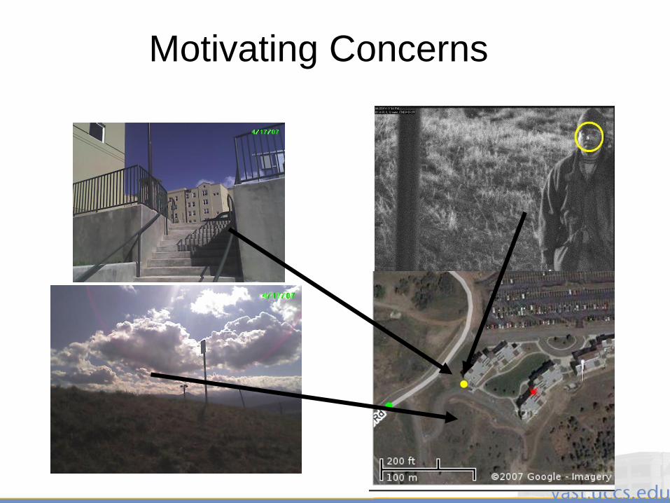
Motivating Concerns

3/28/2011 7
Blur
Lighting
Gamma
NoiseAtmosphere/Weather
Compression
Resolution Sensor / Imaging
Effects
Dynamic Range
Motivating Concerns
3/28/2011 8
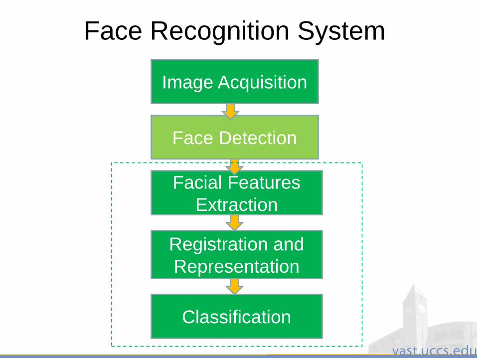
Face Recognition System
Image Acquisition
Face Detection
Facial Features
Extraction
Registration and
Representation
Classification

3/28/2011 9
Face Recognition in our daily life
• Google‟s picasa
• Apples iPhoto
• Facebook Face Recognition
• Windows Live Photo gallery
• Lots of face recognition login software
• Face recognition mobile apps
How is surveillance different?
3/28/2011 10
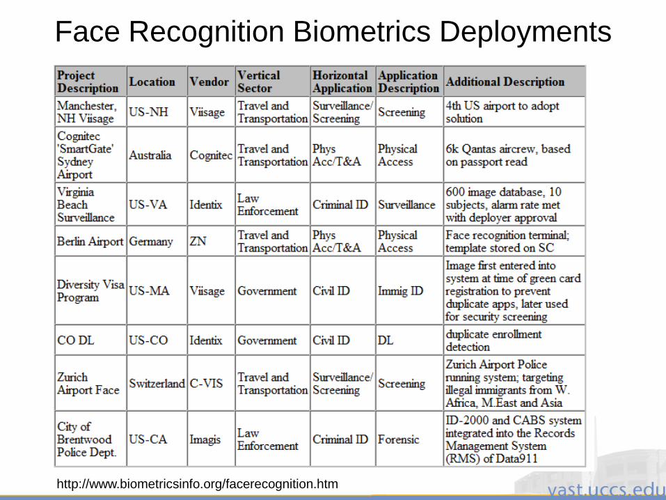
Face Recognition Biometrics Deployments
http://www.biometricsinfo.org/facerecognition.htm
3/28/2011 11
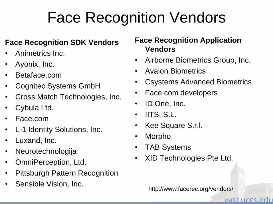
Face Recognition Vendors
Face Recognition SDK Vendors
• Animetrics Inc.
• Ayonix, Inc.
• Betaface.com
• Cognitec Systems GmbH
• Cross Match Technologies, Inc.
• Cybula Ltd.
• Face.com
• L-1 Identity Solutions, Inc.
• Luxand, Inc.
• Neurotechnologija
• OmniPerception, Ltd.
• Pittsburgh Pattern Recognition
• Sensible Vision, Inc.
Face Recognition Application
Vendors
• Airborne Biometrics Group, Inc.
• Avalon Biometrics
• Csystems Advanced Biometrics
• Face.com developers
• ID One, Inc.
• IITS, S.L.
• Kee Square S.r.l.
• Morpho
• TAB Systems
• XID Technologies Pte Ltd.
http://www.facerec.org/vendors/
3/28/2011 12
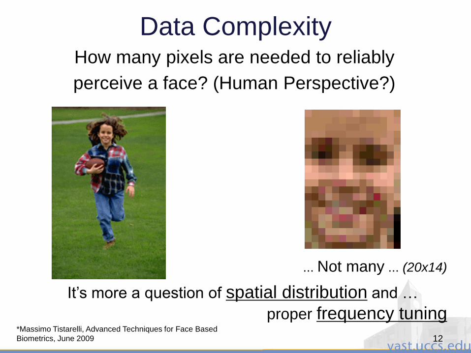
Data Complexity
... Not many ... (20x14)
It‟s more a question of spatial distribution and …
proper frequency tuning
12
How many pixels are needed to reliably
perceive a face? (Human Perspective?)
*Massimo Tistarelli, Advanced Techniques for Face Based
Biometrics, June 2009
3/28/2011 13
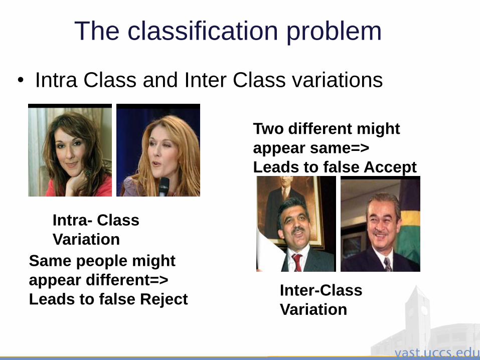
The classification problem
• Intra Class and Inter Class variations
Intra- Class
Variation
Inter-Class
Variation
Same people might
appear different=>
Leads to false Reject
Two different might
appear same=>
Leads to false Accept
3/28/2011 14
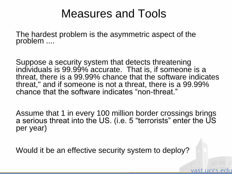
Measures and Tools
The hardest problem is the asymmetric aspect of the problem ....
Suppose a security system that detects threatening individuals is 99.99% accurate. That is, if someone is a threat, there is a 99.99% chance that the software indicates threat," and if someone is not a threat, there is a 99.99% chance that the software indicates “non-threat.”
Assume that 1 in every 100 million border crossings brings a serious threat into the US. (i.e. 5 “terrorists” enter the US per year)
Would it be an effective security system to deploy?
3/28/2011 15
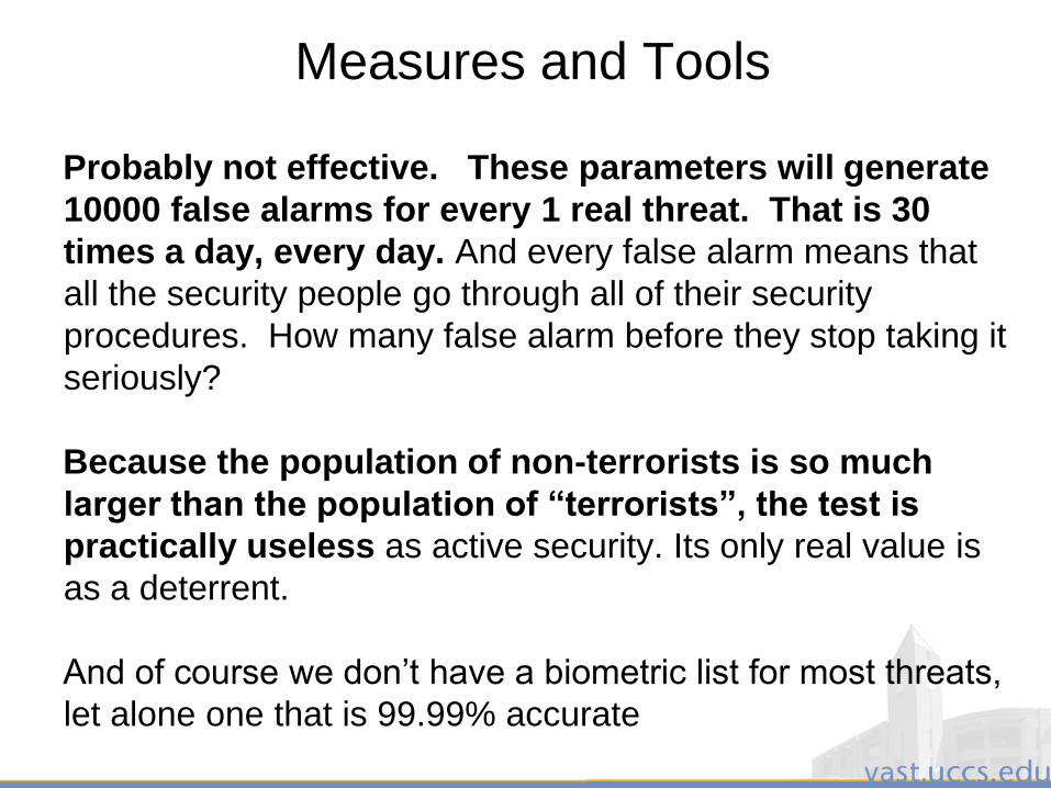
Measures and Tools
Probably not effective. These parameters will generate
10000 false alarms for every 1 real threat. That is 30
times a day, every day. And every false alarm means that
all the security people go through all of their security
procedures. How many false alarm before they stop taking it
seriously?
Because the population of non-terrorists is so much
larger than the population of “terrorists”, the test is
practically useless as active security. Its only real value is
as a deterrent.
And of course we don‟t have a biometric list for most threats,
let alone one that is 99.99% accurate
3/28/2011 16
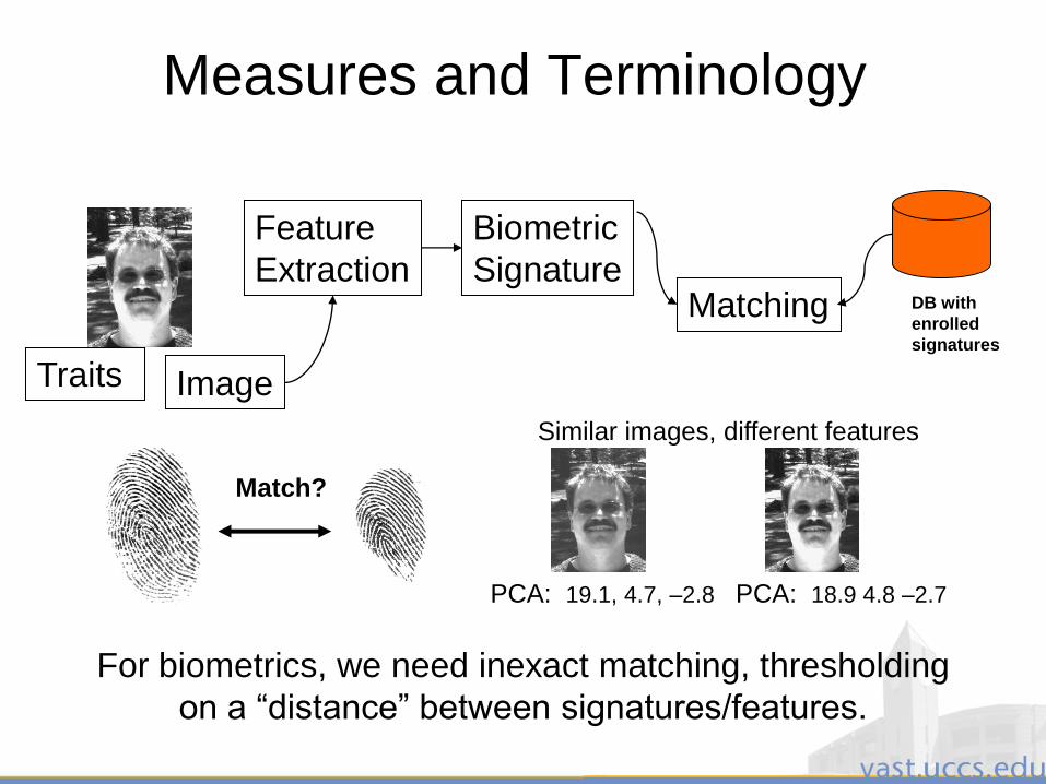
Measures and Terminology
Similar images, different features
PCA: 19.1, 4.7, –2.8 PCA: 18.9 4.8 –2.7
For biometrics, we need inexact matching, thresholding
on a “distance” between signatures/features.
Traits Image
Feature
Extraction
Biometric
SignatureMatching DB with
enrolled
signatures
Match?
3/28/2011 17
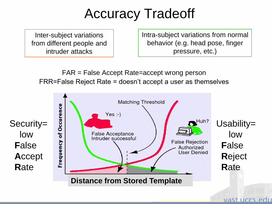
Accuracy Tradeoff
FAR = False Accept Rate=accept wrong person
FRR=False Reject Rate = doesn‟t accept a user as themselves
Intra-subject variations from normal
behavior (e.g. head pose, finger
pressure, etc.)
Inter-subject variations
from different people and
intruder attacks
Security=
low
False
Accept
Rate
Usability=
low
False
Reject
Rate
Distance from Stored Template
3/28/2011 18
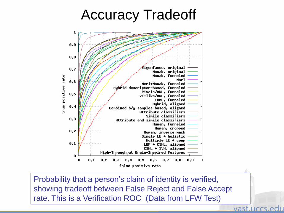
Probability that a person‟s claim of identity is verified,
showing tradeoff between False Reject and False Accept
rate. This is a Verification ROC (Data from LFW Test)
Accuracy Tradeoff
3/28/2011 19
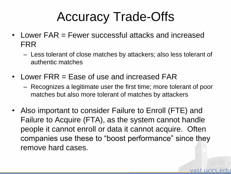
Accuracy Trade-Offs
• Lower FAR = Fewer successful attacks and increased
FRR
– Less tolerant of close matches by attackers; also less tolerant of
authentic matches
• Lower FRR = Ease of use and increased FAR
– Recognizes a legitimate user the first time; more tolerant of poor
matches but also more tolerant of matches by attackers
• Also important to consider Failure to Enroll (FTE) and
Failure to Acquire (FTA), as the system cannot handle
people it cannot enroll or data it cannot acquire. Often
companies use these to “boost performance” since they
remove hard cases.
3/28/2011 20
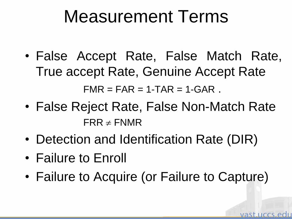
Measurement Terms
• False Accept Rate, False Match Rate,
True accept Rate, Genuine Accept Rate
FMR = FAR = 1-TAR = 1-GAR .
• False Reject Rate, False Non-Match RateFRR FNMR
• Detection and Identification Rate (DIR)
• Failure to Enroll
• Failure to Acquire (or Failure to Capture)
3/28/2011 21
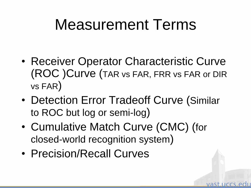
Measurement Terms
• Receiver Operator Characteristic Curve (ROC )Curve (TAR vs FAR, FRR vs FAR or DIR
vs FAR)
• Detection Error Tradeoff Curve (Similar
to ROC but log or semi-log)
• Cumulative Match Curve (CMC) (for
closed-world recognition system)
• Precision/Recall Curves
3/28/2011 22
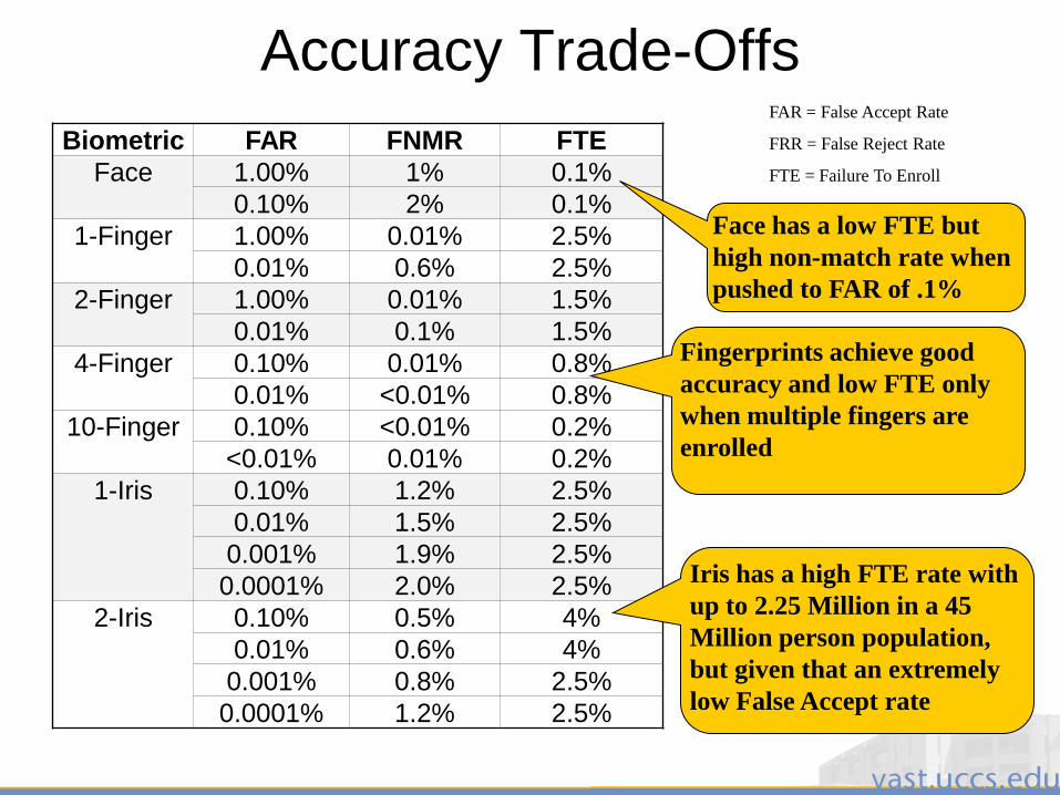
Accuracy Trade-Offs
Biometric FAR FNMR FTE
Face 1.00% 1% 0.1%
0.10% 2% 0.1%
1-Finger 1.00% 0.01% 2.5%
0.01% 0.6% 2.5%
2-Finger 1.00% 0.01% 1.5%
0.01% 0.1% 1.5%
4-Finger 0.10% 0.01% 0.8%
0.01% <0.01% 0.8%
10-Finger 0.10% <0.01% 0.2%
<0.01% 0.01% 0.2%
1-Iris 0.10% 1.2% 2.5%
0.01% 1.5% 2.5%
0.001% 1.9% 2.5%
0.0001% 2.0% 2.5%
2-Iris 0.10% 0.5% 4%
0.01% 0.6% 4%
0.001% 0.8% 2.5%
0.0001% 1.2% 2.5%
Iris has a high FTE rate with
up to 2.25 Million in a 45
Million person population,
but given that an extremely
low False Accept rate
Fingerprints achieve good
accuracy and low FTE only
when multiple fingers are
enrolled
Face has a low FTE but
high non-match rate when
pushed to FAR of .1%
FAR = False Accept Rate
FRR = False Reject Rate
FTE = Failure To Enroll
3/28/2011 23
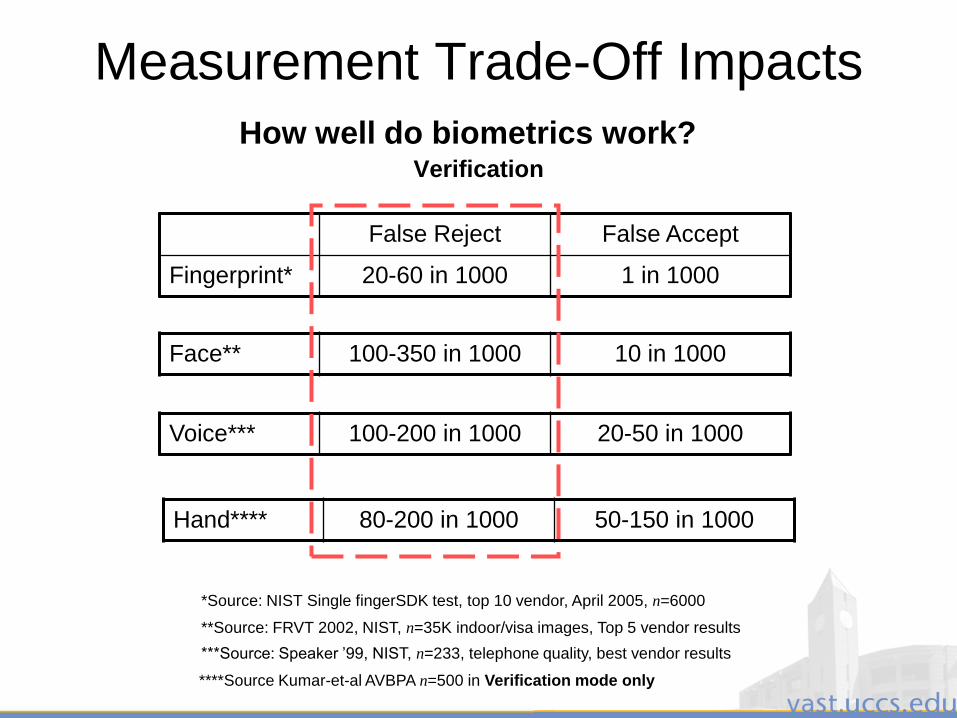
How well do biometrics work?Verification
False Reject False Accept
Fingerprint* 20-60 in 1000 1 in 1000
*Source: NIST Single fingerSDK test, top 10 vendor, April 2005, n=6000
Face** 100-350 in 1000 10 in 1000
**Source: FRVT 2002, NIST, n=35K indoor/visa images, Top 5 vendor results
Voice*** 100-200 in 1000 20-50 in 1000
****Source Kumar-et-al AVBPA n=500 in Verification mode only
Hand**** 80-200 in 1000 50-150 in 1000
Measurement Trade-Off Impacts
***Source: Speaker ‟99, NIST, n=233, telephone quality, best vendor results
3/28/2011 24
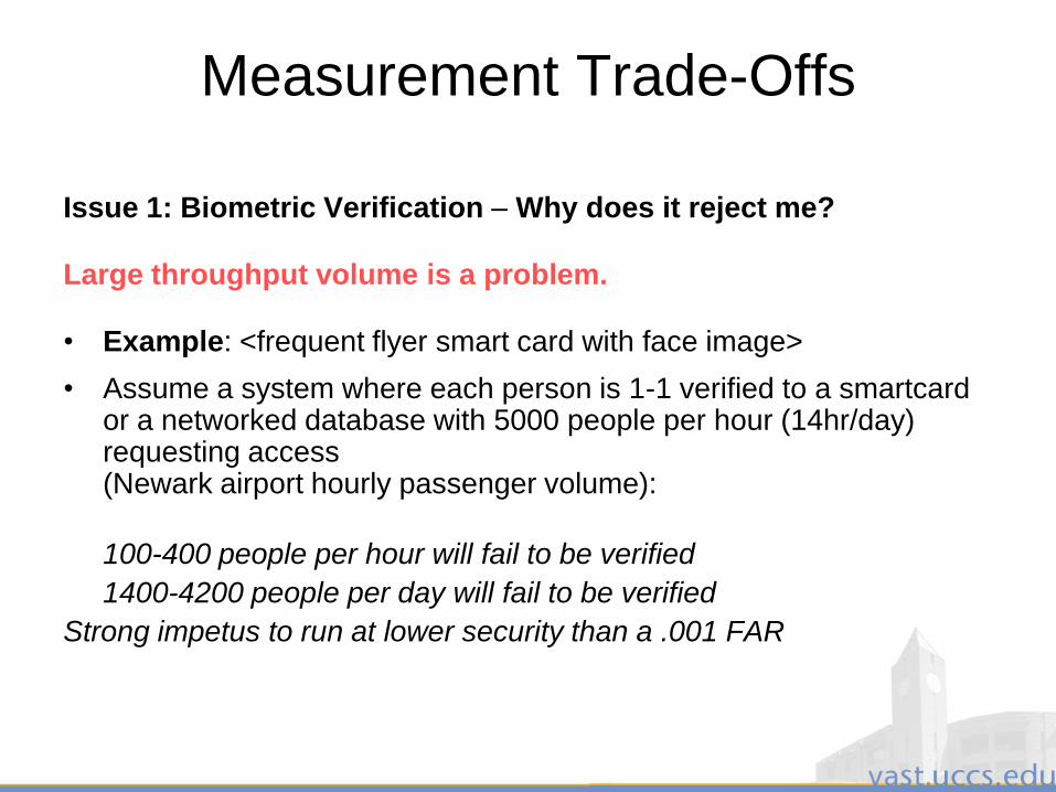
Measurement Trade-Offs
Issue 1: Biometric Verification – Why does it reject me?
Large throughput volume is a problem.
• Example: <frequent flyer smart card with face image>
• Assume a system where each person is 1-1 verified to a smartcard or a networked database with 5000 people per hour (14hr/day) requesting access(Newark airport hourly passenger volume):
100-400 people per hour will fail to be verified
1400-4200 people per day will fail to be verified
Strong impetus to run at lower security than a .001 FAR
3/28/2011 25
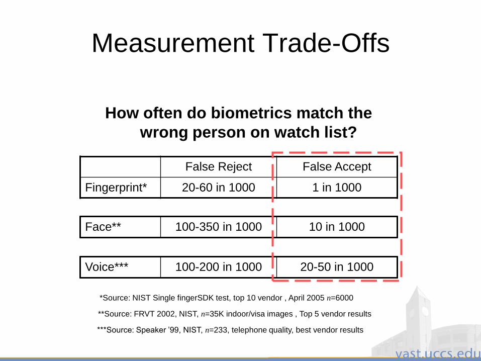
How often do biometrics match the
wrong person on watch list?
False Reject False Accept
Fingerprint* 20-60 in 1000 1 in 1000
*Source: NIST Single fingerSDK test, top 10 vendor , April 2005 n=6000
Face** 100-350 in 1000 10 in 1000
**Source: FRVT 2002, NIST, n=35K indoor/visa images , Top 5 vendor results
Voice*** 100-200 in 1000 20-50 in 1000
***Source: Speaker ‟99, NIST, n=233, telephone quality, best vendor results
Measurement Trade-Offs
3/28/2011 26
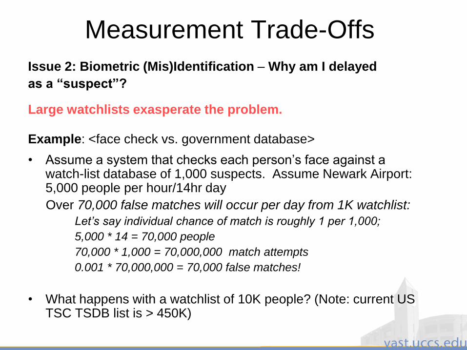
Measurement Trade-Offs
Issue 2: Biometric (Mis)Identification – Why am I delayed
as a “suspect”?
Large watchlists exasperate the problem.
Example: <face check vs. government database>
• Assume a system that checks each person‟s face against a watch-list database of 1,000 suspects. Assume Newark Airport: 5,000 people per hour/14hr day
Over 70,000 false matches will occur per day from 1K watchlist:
Let’s say individual chance of match is roughly 1 per 1,000;
5,000 * 14 = 70,000 people
70,000 * 1,000 = 70,000,000 match attempts
0.001 * 70,000,000 = 70,000 false matches!
• What happens with a watchlist of 10K people? (Note: current US TSC TSDB list is > 450K)
3/28/2011 27
Measurement Trade-Offs
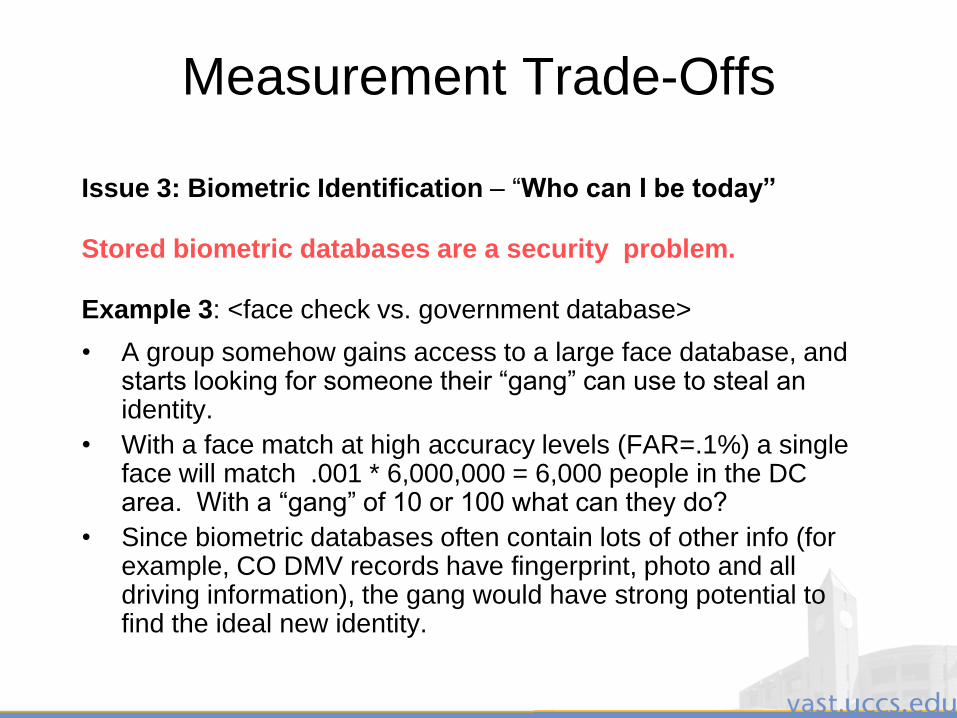
Issue 3: Biometric Identification – “Who can I be today”
Stored biometric databases are a security problem.
Example 3: <face check vs. government database>
• A group somehow gains access to a large face database, and starts looking for someone their “gang” can use to steal an identity.
• With a face match at high accuracy levels (FAR=.1%) a single face will match .001 * 6,000,000 = 6,000 people in the DC area. With a “gang” of 10 or 100 what can they do?
• Since biometric databases often contain lots of other info (for example, CO DMV records have fingerprint, photo and all driving information), the gang would have strong potential to find the ideal new identity.
3/28/2011 28
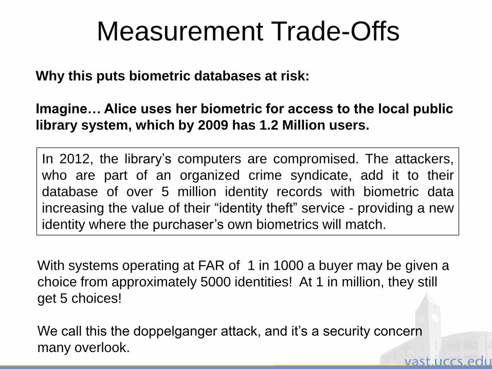
Why this puts biometric databases at risk:
Imagine… Alice uses her biometric for access to the local public
library system, which by 2009 has 1.2 Million users.
In 2012, the library‟s computers are compromised. The attackers,
who are part of an organized crime syndicate, add it to their
database of over 5 million identity records with biometric data
increasing the value of their “identity theft” service - providing a new
identity where the purchaser‟s own biometrics will match.
Measurement Trade-Offs
With systems operating at FAR of 1 in 1000 a buyer may be given a
choice from approximately 5000 identities! At 1 in million, they still
get 5 choices!
We call this the doppelganger attack, and it‟s a security concern
many overlook.
3/28/2011 29
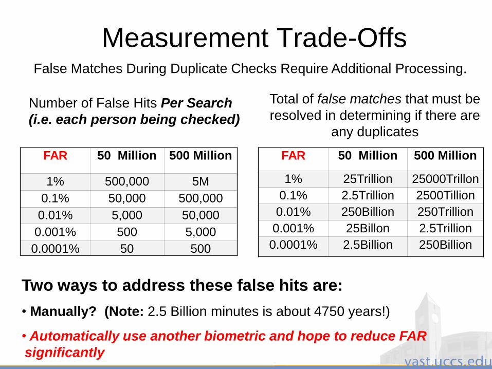
Measurement Trade-Offs
FAR 50 Million 500 Million
1% 500,000 5M
0.1% 50,000 500,000
0.01% 5,000 50,000
0.001% 500 5,000
0.0001% 50 500
Two ways to address these false hits are:
• Manually? (Note: 2.5 Billion minutes is about 4750 years!)
• Automatically use another biometric and hope to reduce FAR
significantly
Number of False Hits Per Search
(i.e. each person being checked)
False Matches During Duplicate Checks Require Additional Processing.
FAR 50 Million 500 Million
1% 25Trillion 25000Trillon
0.1% 2.5Trillion 2500Tillion
0.01% 250Billion 250Trillion
0.001% 25Billon 2.5Trillion
0.0001% 2.5Billion 250Billion
Total of false matches that must be
resolved in determining if there are
any duplicates
3/28/2011 30
Types of Biometric Problems
• We differentiate between biometrics for:– Cooperative applications: user convenience or
limited security (e.g. login) and
– Security applications that address fraud and national issues (e.g. borders, welfare card).
• For personal applications, users want to make it work, for security applications some want to make it fail.
• For security applications you must consider what is your adversary‟s motivation, and what they can do to defeat the system.
3/28/2011 31
Types of Biometric Problems
• Types of Biometric “subjects”– Cooperative: aware of system and trying to make
the system work
– Non-cooperative: not trying to help, or break the system - generally unaware of system being used.
– Adversarial (Uncooperative): aware of the system and trying to defeat it.
– Challenged: Probably trying to be cooperative but with physical/mental challenges.
3/28/2011 32
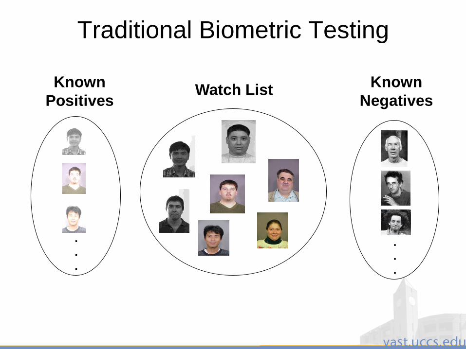
Traditional Biometric Testing
Watch ListKnown
Positives
Known
Negatives
.
.
.
.
.
.
3/28/2011 33
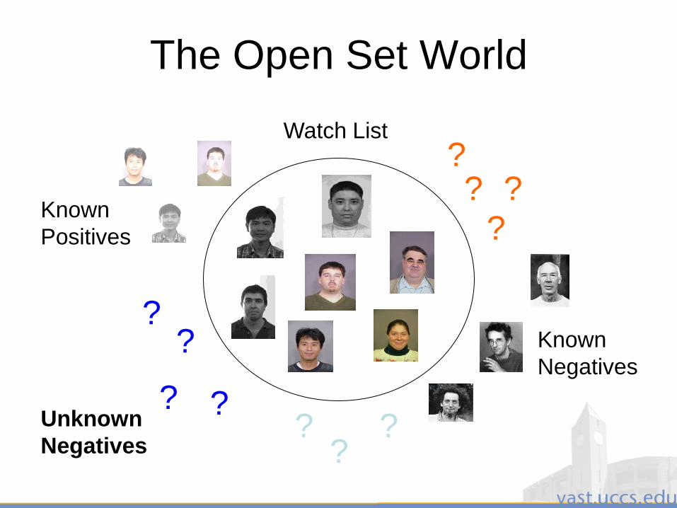
The Open Set World
Watch List
?
??
??
??Unknown
Negatives
? ??
?
Known
Positives
Known
Negatives
3/28/2011 34
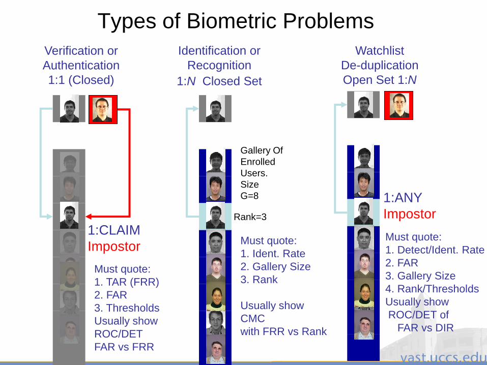
Types of Biometric Problems
Identification or
Recognition
1:N Closed Set
Verification or
Authentication
1:1 (Closed)
1:CLAIM
Impostor
Watchlist
De-duplication
Open Set 1:N
1:ANY
ImpostorRank=3
Gallery Of
Enrolled
Users.
Size
G=8
Must quote:
1. Ident. Rate
2. Gallery Size
3. Rank
Usually show
CMC
with FRR vs Rank
Must quote:
1. TAR (FRR)
2. FAR
3. Thresholds
Usually show
ROC/DET
FAR vs FRR
Must quote:
1. Detect/Ident. Rate
2. FAR
3. Gallery Size
4. Rank/Thresholds
Usually show
ROC/DET of
FAR vs DIR
3/28/2011 35
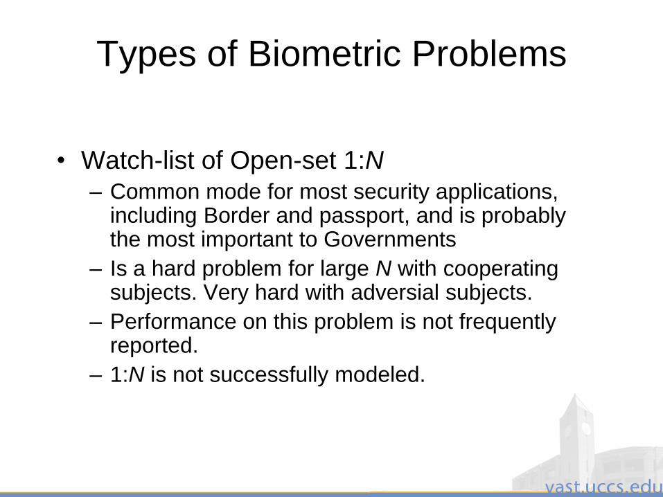
Types of Biometric Problems
• Watch-list of Open-set 1:N– Common mode for most security applications,
including Border and passport, and is probably the most important to Governments
– Is a hard problem for large N with cooperating subjects. Very hard with adversial subjects.
– Performance on this problem is not frequently reported.
– 1:N is not successfully modeled.

3/28/2011 36
Addressing the Problem of Unknown Negatives*
• A probe pj is recognized if the correct match
score is above an operating threshold τ
– Rank(pj) = 1
– s∗j ≥ τ for the similarity match where id(pj) = id(g*)
• A false alarm occurs when the top match score
for an impostor is above the operating threshold
– max sij ≥ τ
*P. Phillips, P. Grother, R. Micheals, “Evaluation Methods in Face Recognition,” 2005.

3/28/2011 37
Acquisition Considerations
3/28/2011 38
Lighting Considerations
• How much light, and how to measure it?
– Illuminance vs luminance
• Illuminance (lux) varies significantly across the
population, is impacted by directional reflection,
and, in general, can only be measured to .01lux
• Luminance (candela per m2, or nit) describes the
“brightness” of the source, and does not vary
with distance

3/28/2011 39
Lighting Considerations
• “Sky Quality” meter - measurements in
Magnitudes/arcsecond.
Conversion to nits:cd
m2= 108000 x 10-0.4*s
s is value
produced by
sky quality
meter
A different approach to measuring luminance:
3/28/2011 40
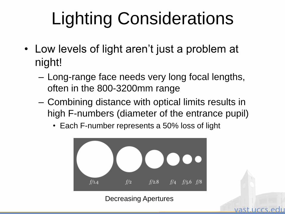
Lighting Considerations
• Low levels of light aren‟t just a problem at
night!
– Long-range face needs very long focal lengths,
often in the 800-3200mm range
– Combining distance with optical limits results in
high F-numbers (diameter of the entrance pupil)
• Each F-number represents a 50% loss of light
Decreasing Apertures
3/28/2011 41
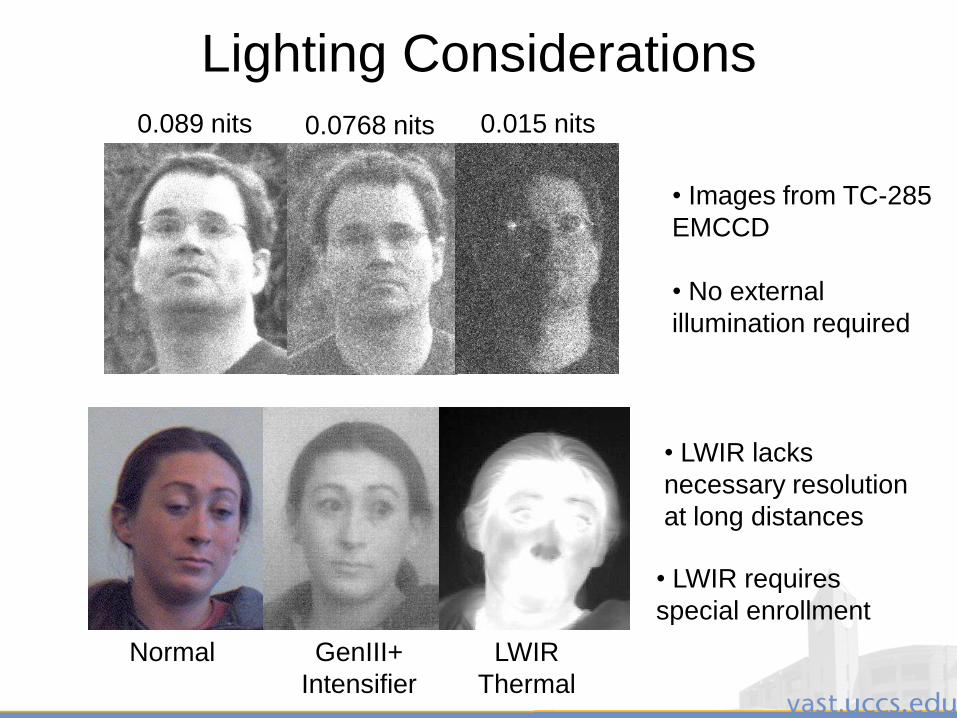
Lighting Considerations0.089 nits 0.0768 nits 0.015 nits
Normal GenIII+
Intensifier
LWIR
Thermal
• LWIR requires
special enrollment
• LWIR lacks
necessary resolution
at long distances
• Images from TC-285
EMCCD
• No external
illumination required
3/28/2011 42
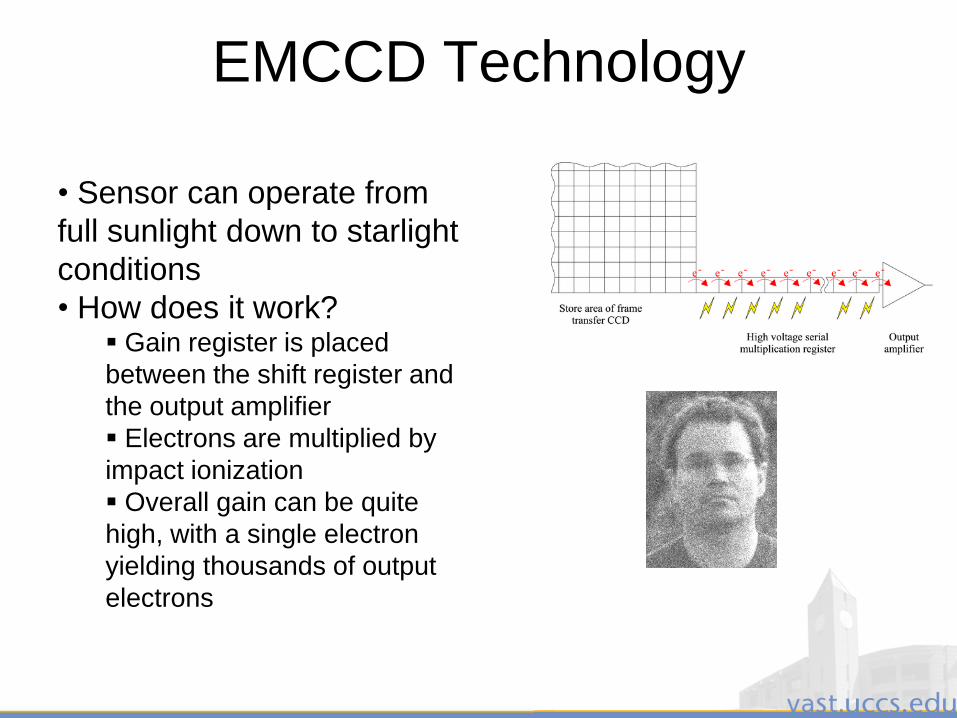
EMCCD Technology
• Sensor can operate from
full sunlight down to starlight
conditions
• How does it work? Gain register is placed
between the shift register and
the output amplifier
Electrons are multiplied by
impact ionization
Overall gain can be quite
high, with a single electron
yielding thousands of output
electrons

3/28/2011 43
EMCCD at Quarter Moonlight Conditions
3/28/2011 44
Sensor/Optics Considerations
• Effective resolution is more than just the number of
pixels
• Modulation Transfer Function
– Accounts for blur and contrast loss
– Optical MTF x Sensor Geometry MTF x Diffusion MTF
– MTF values above 0.6 are considered satisfactory
• Examples
– Canon EF 400mm f2.8 IS USM: MTF above 9.0 over the
whole field of view
– Same setup with Canon 2xII extender: MTF above 7.0

3/28/2011 45
Lens Considerations
• The ability of a lens to resolve detail is usually
determined by the quality of the lens
– High quality lenses are diffraction limited
– If a lens is not diffraction limited, artifacts can
occur
• Different rays
leaving a single
scene point do not
arrive at single point
on the sensor
• Ideally, the circle of confusion will be smaller than a sensor pixel

3/28/2011 46
Optics / Sensor Matching
• Lenses are multiple-element multi-coated
designs optimized for particular sensors and
wavelengths
– Watch out for vignetting, spatially varying blur, and
color “fringe” artifacts
3/28/2011 47
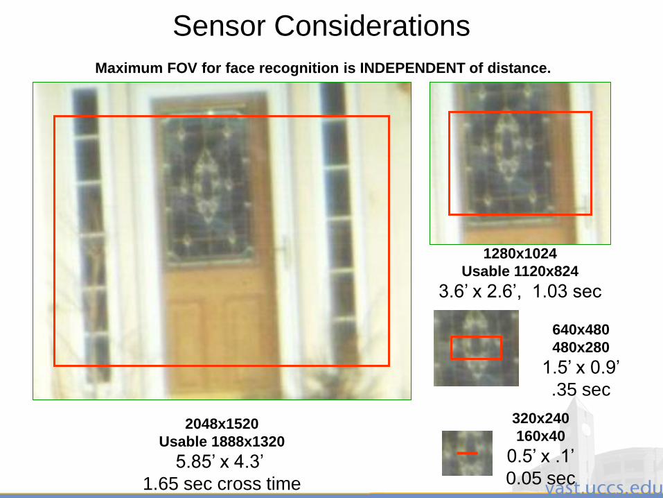
Sensor Considerations
2048x1520
Usable 1888x1320
5.85‟ x 4.3‟
1.65 sec cross time
1280x1024
Usable 1120x824
3.6‟ x 2.6‟, 1.03 sec
640x480
480x280
1.5‟ x 0.9‟
.35 sec
320x240
160x40
0.5‟ x .1‟
0.05 sec
Maximum FOV for face recognition is INDEPENDENT of distance.
3/28/2011 48
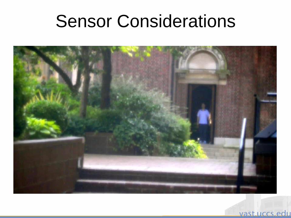
Sensor Considerations
3/28/2011 49
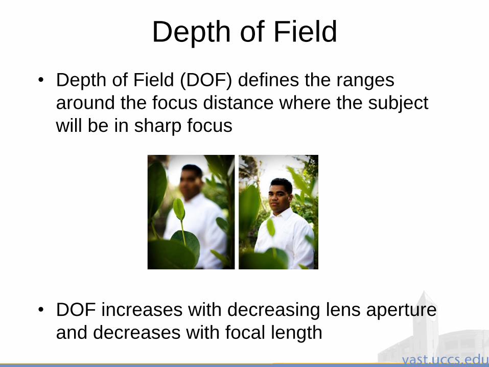
Depth of Field
• Depth of Field (DOF) defines the ranges
around the focus distance where the subject
will be in sharp focus
• DOF increases with decreasing lens aperture
and decreases with focal length
3/28/2011 50
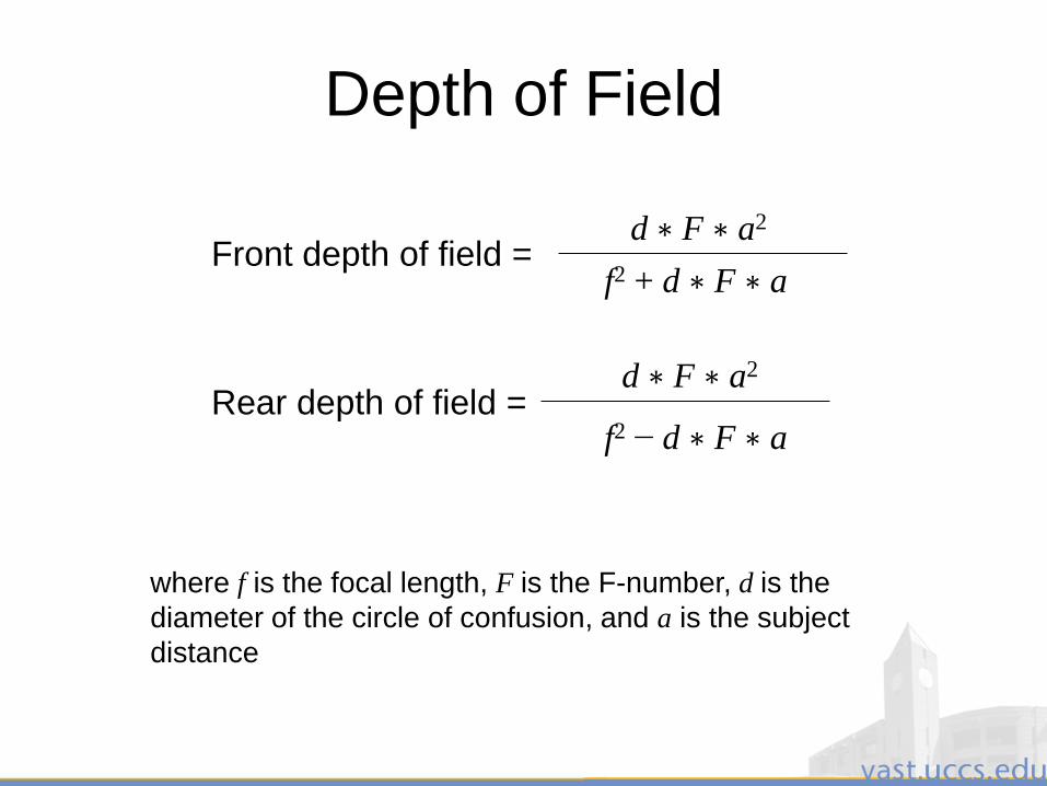
Depth of Field
Front depth of field =
Rear depth of field =
d ∗ F ∗ a2
f2 + d ∗ F ∗ a
d ∗ F ∗ a2
f2 − d ∗ F ∗ a
where f is the focal length, F is the F-number, d is the
diameter of the circle of confusion, and a is the subject
distance

3/28/2011 51
Sensor Considerations
1280
640
320
Choke-Point FOV and timing
3/28/2011 52
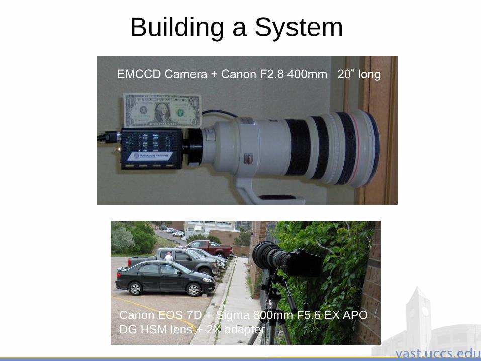
Building a System
EMCCD Camera + Canon F2.8 400mm 20” long
Canon EOS 7D + Sigma 800mm F5.6 EX APO
DG HSM lens + 2X adapter

3/28/2011 53
Sensor Considerations
Typical motion blur
• Images taken approximately 100M from the EMCCD
camera at dusk
• Top of the walking stride produces minimal blur
(~0.4 lux, yielding face lumens of 0.115 nits)
3/28/2011 54
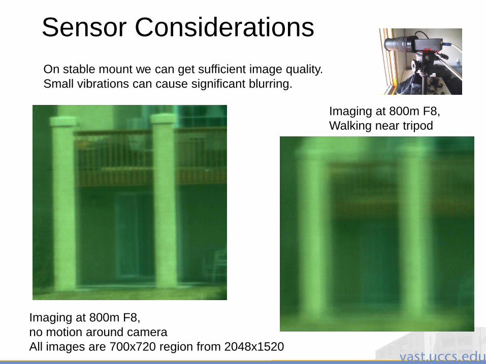
Sensor Considerations
On stable mount we can get sufficient image quality.
Small vibrations can cause significant blurring.
Imaging at 800m F8,
no motion around camera
All images are 700x720 region from 2048x1520
Imaging at 800m F8,
Walking near tripod
3/28/2011 55
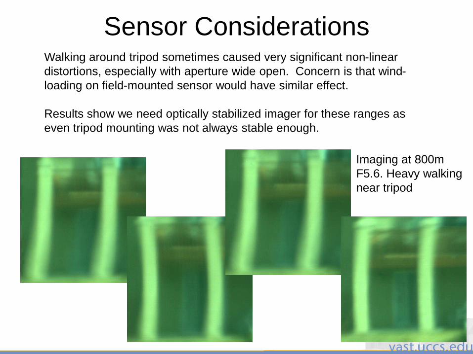
Sensor ConsiderationsWalking around tripod sometimes caused very significant non-linear
distortions, especially with aperture wide open. Concern is that wind-
loading on field-mounted sensor would have similar effect.
Results show we need optically stabilized imager for these ranges as
even tripod mounting was not always stable enough.
Imaging at 800m
F5.6. Heavy walking
near tripod
3/28/2011 56
Sensor Considerations
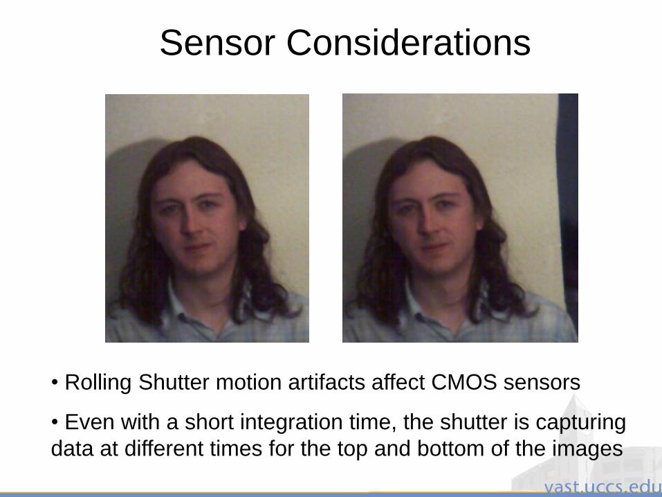
• Rolling Shutter motion artifacts affect CMOS sensors
• Even with a short integration time, the shutter is capturing
data at different times for the top and bottom of the images
3/28/2011 57
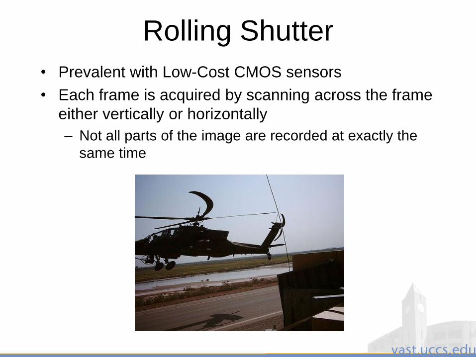
Rolling Shutter
• Prevalent with Low-Cost CMOS sensors
• Each frame is acquired by scanning across the frame
either vertically or horizontally
– Not all parts of the image are recorded at exactly the
same time
3/28/2011 58
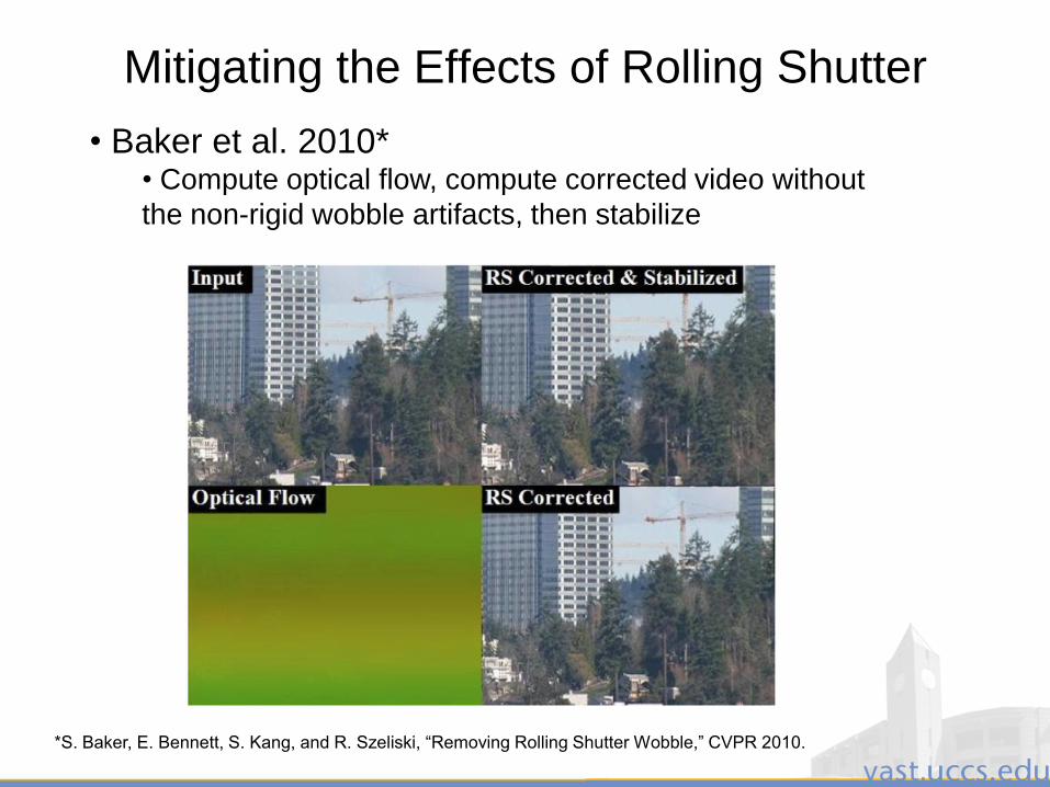
Mitigating the Effects of Rolling Shutter
• Baker et al. 2010*• Compute optical flow, compute corrected video without
the non-rigid wobble artifacts, then stabilize
*S. Baker, E. Bennett, S. Kang, and R. Szeliski, “Removing Rolling Shutter Wobble,” CVPR 2010.
3/28/2011 59
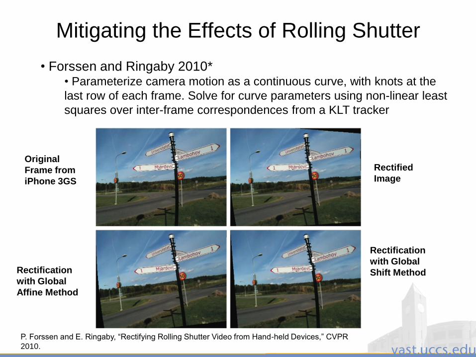
Mitigating the Effects of Rolling Shutter
• Forssen and Ringaby 2010*• Parameterize camera motion as a continuous curve, with knots at the
last row of each frame. Solve for curve parameters using non-linear least
squares over inter-frame correspondences from a KLT tracker
Original
Frame from
iPhone 3GS
Rectified
Image
Rectification
with Global
Affine Method
Rectification
with Global
Shift Method
P. Forssen and E. Ringaby, “Rectifying Rolling Shutter Video from Hand-held Devices,” CVPR
2010.
3/28/2011 60
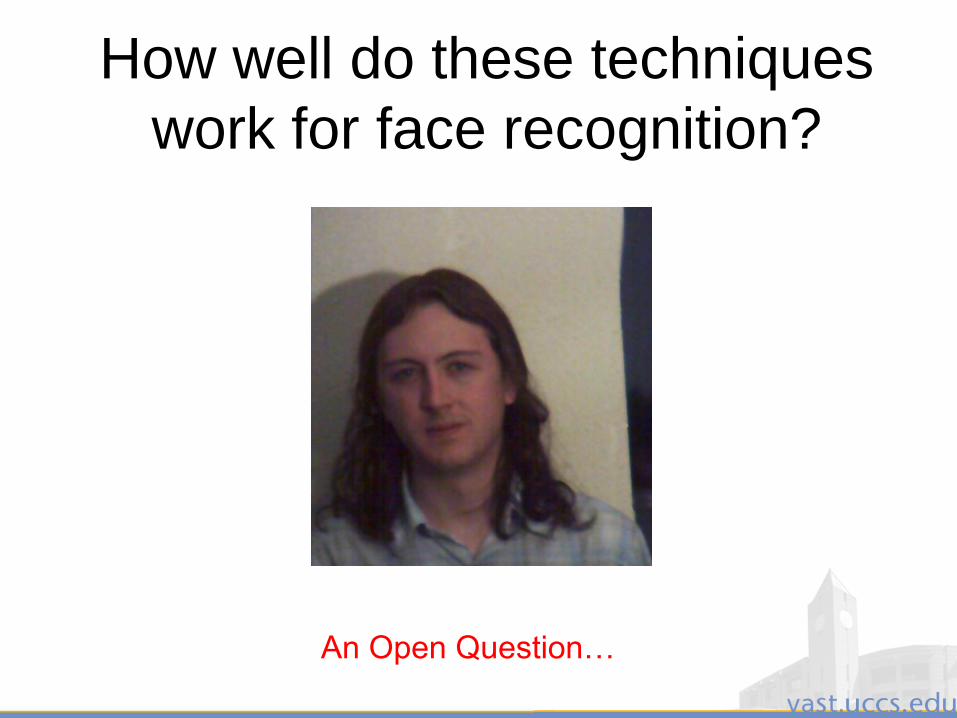
How well do these techniques
work for face recognition?
An Open Question…
3/28/2011 61
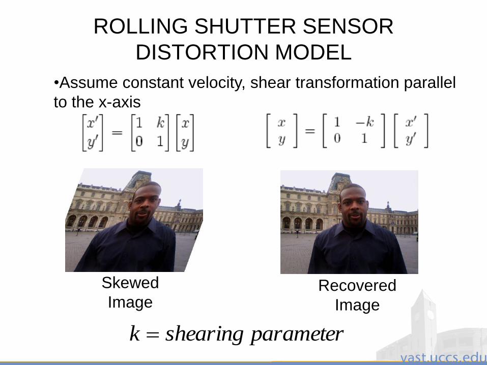
ROLLING SHUTTER SENSOR
DISTORTION MODEL
Recovered
Image
•Assume constant velocity, shear transformation parallel
to the x-axis
Skewed
Image
parametershearingk
3/28/2011 62
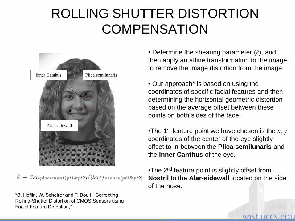
ROLLING SHUTTER DISTORTION
COMPENSATION
• Determine the shearing parameter (k), and
then apply an affine transformation to the image
to remove the image distortion from the image.
• Our approach* is based on using the
coordinates of specific facial features and then
determining the horizontal geometric distortion
based on the average offset between these
points on both sides of the face.
•The 1st feature point we have chosen is the x; y
coordinates of the center of the eye slightly
offset to in-between the Plica semilunaris and
the Inner Canthus of the eye.
•The 2nd feature point is slightly offset from
Nostril to the Alar-sidewall located on the side
of the nose.
*B. Heflin, W. Scheirer and T. Boult, “Correcting
Rolling-Shutter Distortion of CMOS Sensors using
Facial Feature Detection,”
3/28/2011 63
ROLLING SHUTTER DISTORTION
COMPENSATION
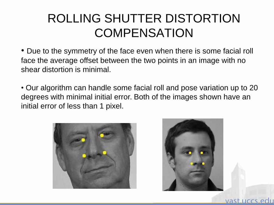
• Due to the symmetry of the face even when there is some facial roll
face the average offset between the two points in an image with no
shear distortion is minimal.
• Our algorithm can handle some facial roll and pose variation up to 20
degrees with minimal initial error. Both of the images shown have an
initial error of less than 1 pixel.
3/28/2011 64
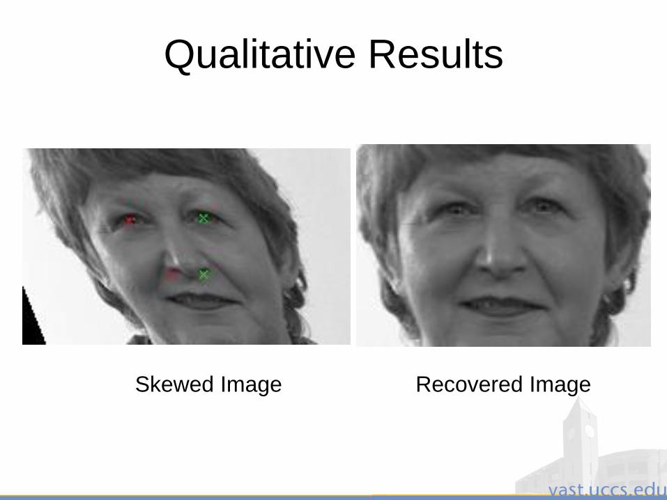
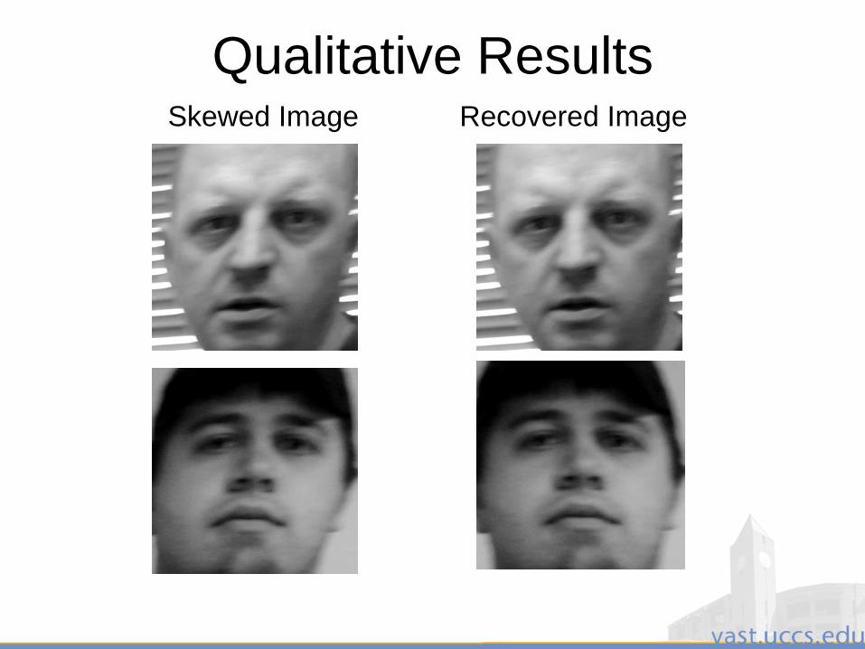
Qualitative Results
Skewed Image Recovered Image
3/28/2011 65
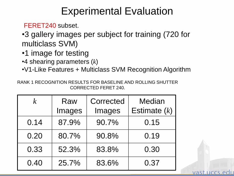
Experimental Evaluation
FERET240 subset.
•3 gallery images per subject for training (720 for
multiclass SVM)
•1 image for testing•4 shearing parameters (k)
•V1-Like Features + Multiclass SVM Recognition Algorithm
k Raw
Images
Corrected
Images
Median
Estimate (k)
0.14 87.9% 90.7% 0.15
0.20 80.7% 90.8% 0.19
0.33 52.3% 83.8% 0.30
0.40 25.7% 83.6% 0.37
RANK 1 RECOGNITION RESULTS FOR BASELINE AND ROLLING SHUTTER
CORRECTED FERET 240.
3/28/2011 66
Qualitative ResultsSkewed Image Recovered Image
3/28/2011 67
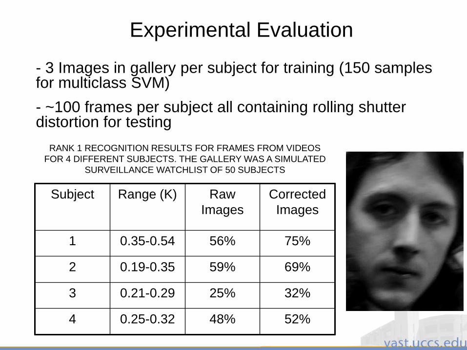
Experimental Evaluation
- 3 Images in gallery per subject for training (150 samples for multiclass SVM)
- ~100 frames per subject all containing rolling shutter distortion for testing
Subject Range (K) Raw
Images
Corrected
Images
1 0.35-0.54 56% 75%
2 0.19-0.35 59% 69%
3 0.21-0.29 25% 32%
4 0.25-0.32 48% 52%
RANK 1 RECOGNITION RESULTS FOR FRAMES FROM VIDEOS
FOR 4 DIFFERENT SUBJECTS. THE GALLERY WAS A SIMULATED
SURVEILLANCE WATCHLIST OF 50 SUBJECTS

3/28/2011 68
Data for Evaluation
3/28/2011 69
Face Databases
The appearance of a face is affected by many factors– Identity
– Face pose - Occlusion
– Illumination - Facial hair
– Facial expression
The development of algorithms robust to these variations requires databases of sufficient size that include carefully controlled variations of these factors.
Common databases are necessary to comparatively evaluate algorithms.
Collecting a high quality database is a resource-intensive task.
3/28/2011 70
Face Databases:AR
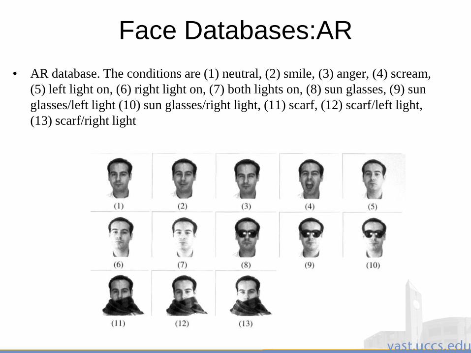
• AR database. The conditions are (1) neutral, (2) smile, (3) anger, (4) scream,
(5) left light on, (6) right light on, (7) both lights on, (8) sun glasses, (9) sun
glasses/left light (10) sun glasses/right light, (11) scarf, (12) scarf/left light,
(13) scarf/right light
3/28/2011 71
Face Databases: CAS-PEAL
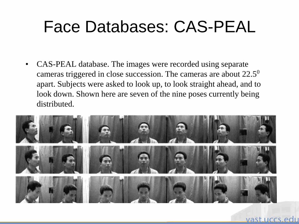
• CAS-PEAL database. The images were recorded using separate
cameras triggered in close succession. The cameras are about 22.50
apart. Subjects were asked to look up, to look straight ahead, and to
look down. Shown here are seven of the nine poses currently being
distributed.
3/28/2011 72
Face Databases: FERET
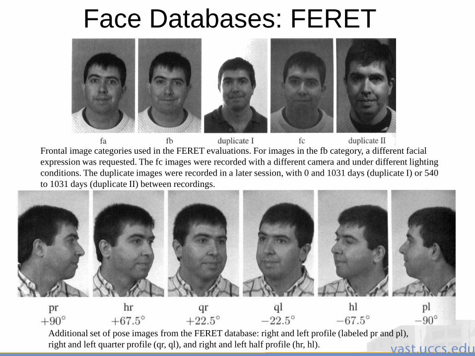
Frontal image categories used in the FERET evaluations. For images in the fb category, a different facial
expression was requested. The fc images were recorded with a different camera and under different lighting
conditions. The duplicate images were recorded in a later session, with 0 and 1031 days (duplicate I) or 540
to 1031 days (duplicate II) between recordings.
Additional set of pose images from the FERET database: right and left profile (labeled pr and pl),
right and left quarter profile (qr, ql), and right and left half profile (hr, hl).

3/28/2011 73
Face Databases: BANCA
The BANCA and XM2VTS video databases distributed by the University of Surrey
3/28/2011 74
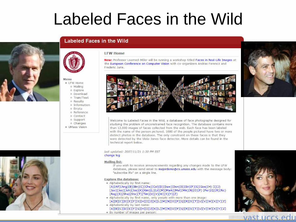
Labeled Faces in the Wild
3/28/2011 75
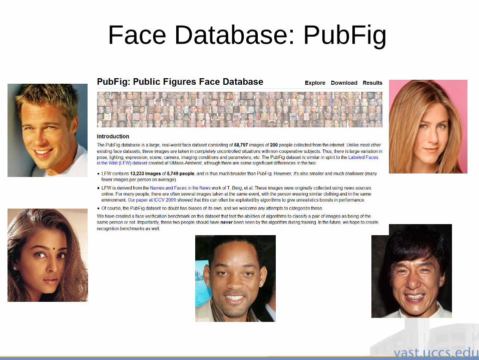
Face Database: PubFig
3/28/2011 76
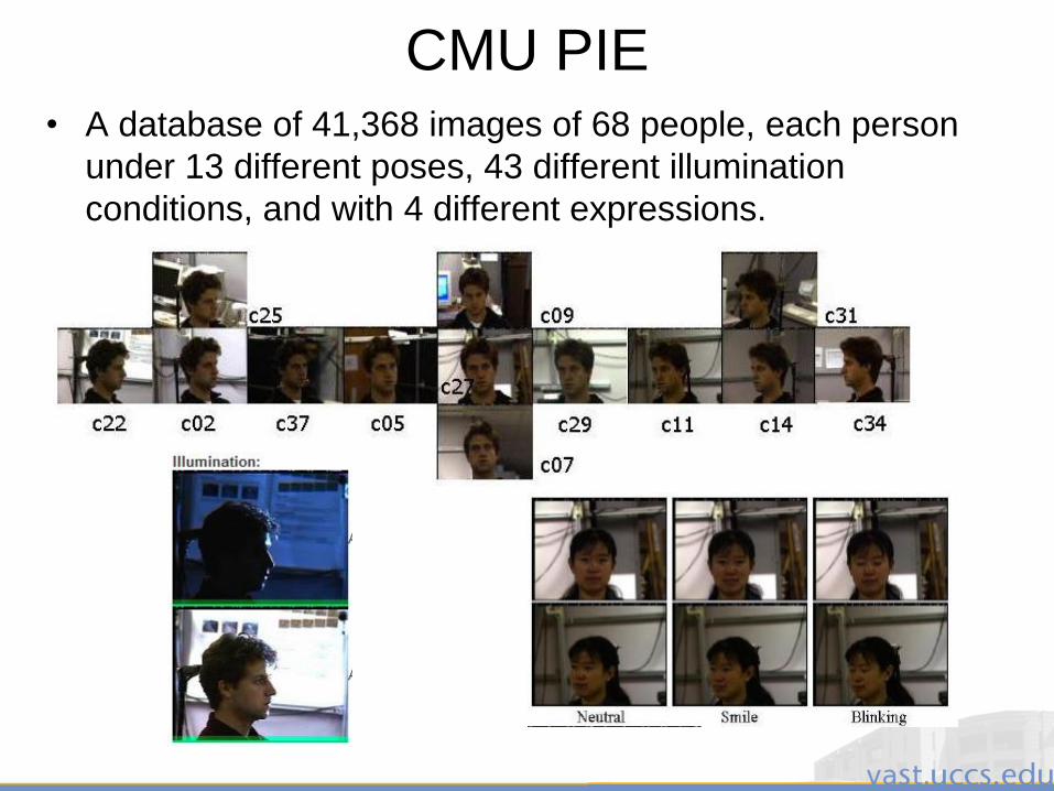
CMU PIE• A database of 41,368 images of 68 people, each person
under 13 different poses, 43 different illumination
conditions, and with 4 different expressions.

3/28/2011 77
ScFace Database
• 4160 static images (in visible and infrared spectrum) of 130 subjects
• 3 distances
• 5 cameras
3/28/2011 78
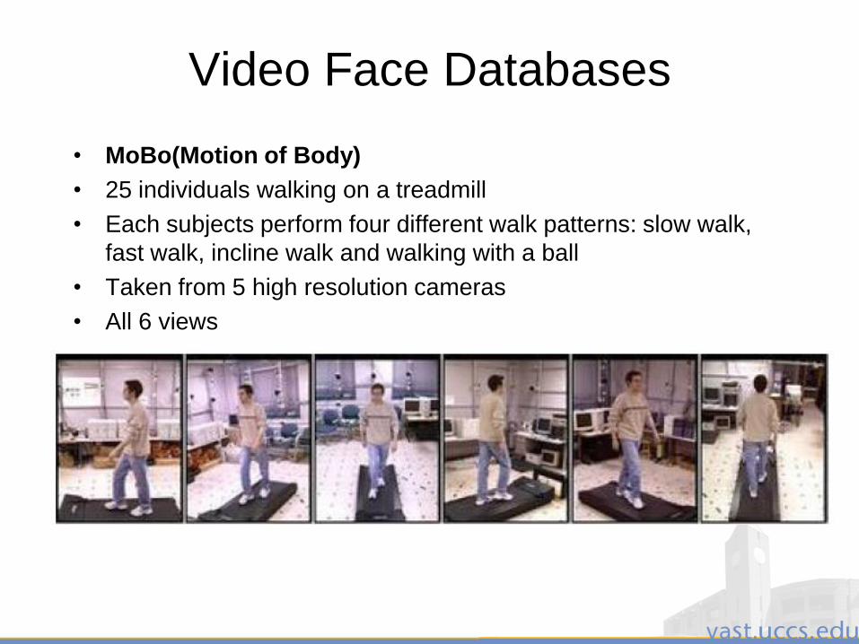
Video Face Databases
• MoBo(Motion of Body)
• 25 individuals walking on a treadmill
• Each subjects perform four different walk patterns: slow walk,
fast walk, incline walk and walking with a ball
• Taken from 5 high resolution cameras
• All 6 views

3/28/2011 79
The Honda/UCSD Database
• Each video sequence is recorded in an indoor environment at 15 frames per second, and each lasted for at least 15 seconds.
• The resolution of each video sequence is 640x480
• Set 1: Training, testing and occlusion subsets contains 20, 42, 13 videos respectively from 20 human subjects.
• Set 2: Training and Testing of 30 videos from another 15 different human subjects
3/28/2011 80
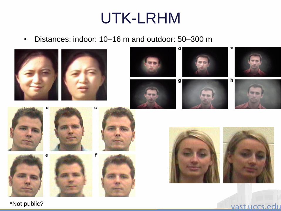
UTK-LRHM
• Distances: indoor: 10–16 m and outdoor: 50–300 m
*Not public?
3/28/2011 81
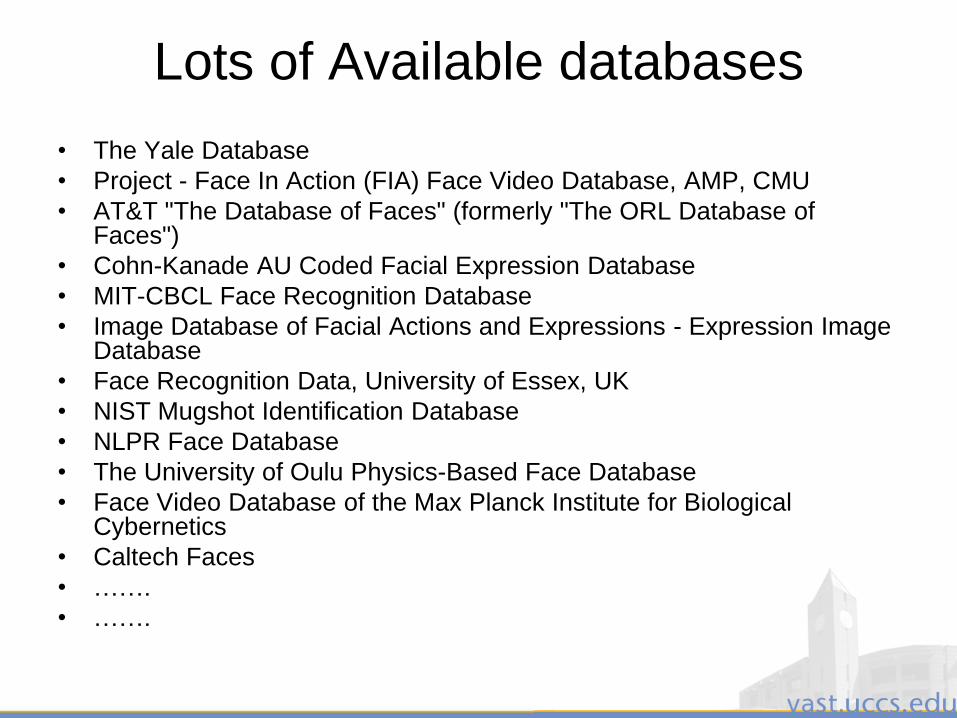
Lots of Available databases
• The Yale Database
• Project - Face In Action (FIA) Face Video Database, AMP, CMU
• AT&T "The Database of Faces" (formerly "The ORL Database of Faces")
• Cohn-Kanade AU Coded Facial Expression Database
• MIT-CBCL Face Recognition Database
• Image Database of Facial Actions and Expressions - Expression Image Database
• Face Recognition Data, University of Essex, UK
• NIST Mugshot Identification Database
• NLPR Face Database
• The University of Oulu Physics-Based Face Database
• Face Video Database of the Max Planck Institute for Biological Cybernetics
• Caltech Faces
• …….
• …….

3/28/2011 82
Requirements of
database/evaluation methods
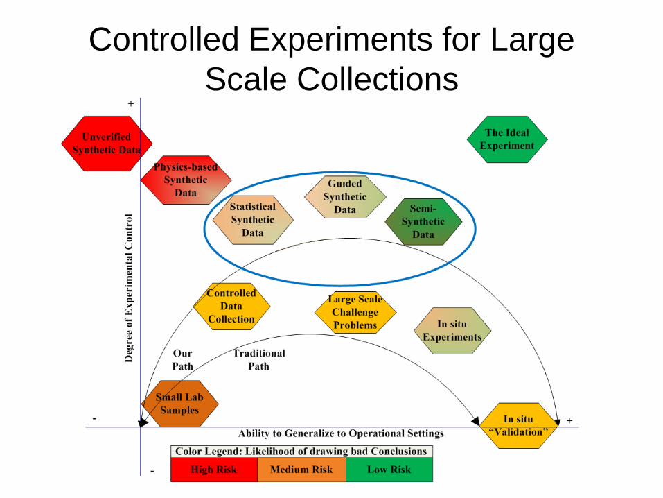
Controlled Experiments for Large
Scale Collections
3/28/2011 84
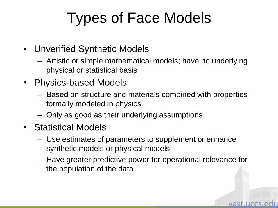
Types of Face Models
• Unverified Synthetic Models
– Artistic or simple mathematical models; have no underlying
physical or statistical basis
• Physics-based Models
– Based on structure and materials combined with properties
formally modeled in physics
– Only as good as their underlying assumptions
• Statistical Models
– Use estimates of parameters to supplement or enhance
synthetic models or physical models
– Have greater predictive power for operational relevance for
the population of the data
3/28/2011 85
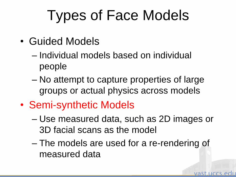
Types of Face Models
• Guided Models
– Individual models based on individual
people
– No attempt to capture properties of large
groups or actual physics across models
• Semi-synthetic Models
– Use measured data, such as 2D images or
3D facial scans as the model
– The models are used for a re-rendering of
measured data

3/28/2011 86
Experiment Setup :
Sensor : FOV 0.5o and 0.25o imaging (equivalent to 1600mm and 3200mm
focal lengths ).
Inter-pupil distance in resulting images is approx 120 pixels
181ft (55m)
91 ft (28m)
Controlled Experiments for Large Scale Collections
Photo-head Data
Acquisition
3/28/2011 87
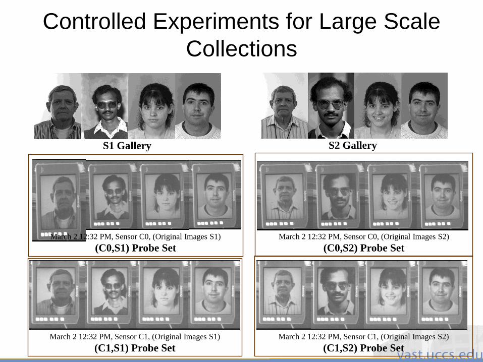
S2 GalleryS1 Gallery
March 2 12:32 PM, Sensor C0, (Original Images S2)
(C0,S2) Probe Set
March 2 12:32 PM, Sensor C0, (Original Images S1)
(C0,S1) Probe Set
March 2 12:32 PM, Sensor C1, (Original Images S2)
(C1,S2) Probe Set
March 2 12:32 PM, Sensor C1, (Original Images S1)
(C1,S1) Probe Set
Controlled Experiments for Large Scale
Collections

3/28/2011 88
Controlled Experiments for Large Scale
Collections
Blur length 15
pixels, 122°Blur length 17
pixels, 59°Blur length 20
pixels, 52°
Lighting:
1/4 Moonlight
0.043 - 0.017 nits
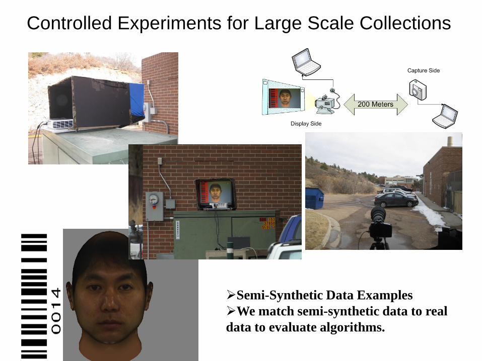
Controlled Experiments for Large Scale Collections
Semi-Synthetic Data Examples
We match semi-synthetic data to real
data to evaluate algorithms.
3/28/2011 90
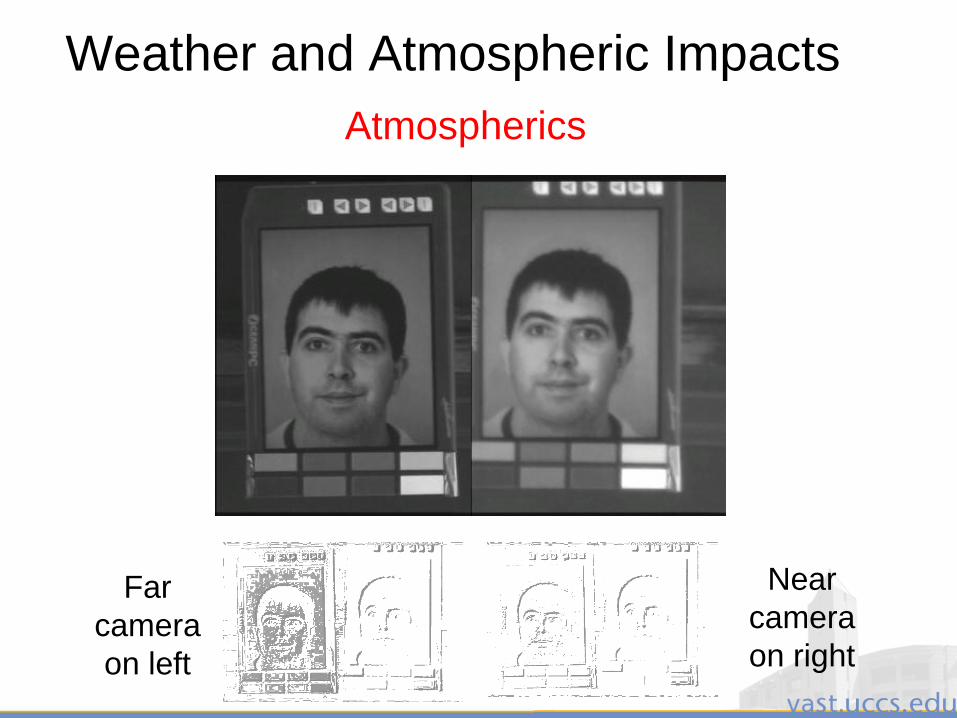
Weather and Atmospheric Impacts
Atmospherics
Far
camera
on left
Near
camera
on right
3/28/2011 91
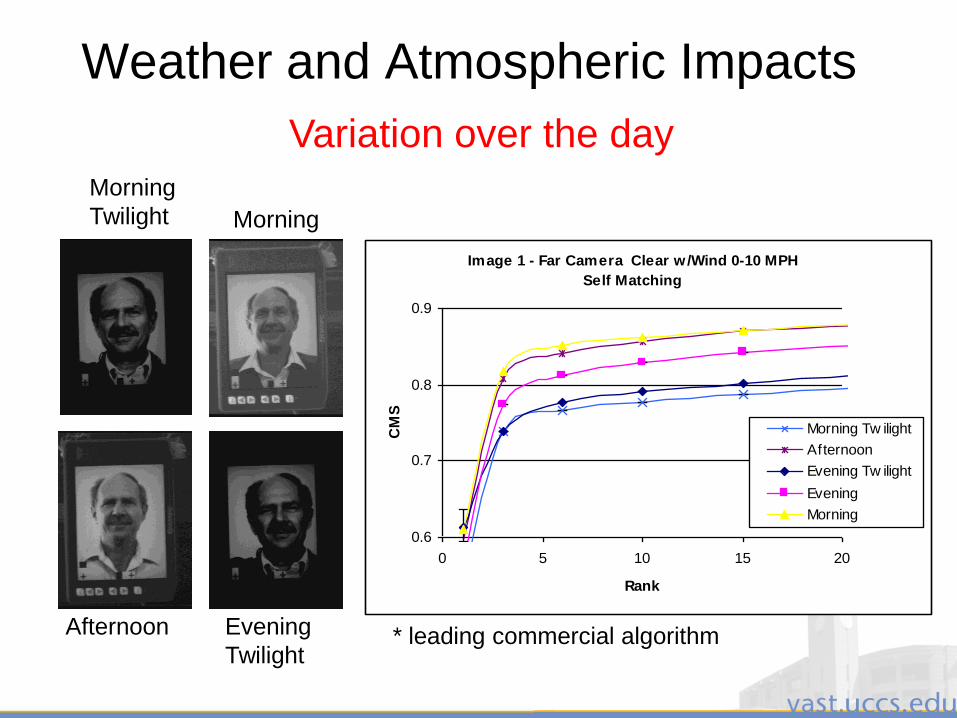
Weather and Atmospheric Impacts
Image 1 - Far Camera Clear w/Wind 0-10 MPH
Self Matching
0.6
0.7
0.8
0.9
0 5 10 15 20
Rank
CM
S
Morning Tw ilight
Afternoon
Evening Tw ilight
Evening
Morning
* leading commercial algorithm
Morning
Twilight Morning
Afternoon Evening
Twilight
Variation over the day
3/28/2011 92
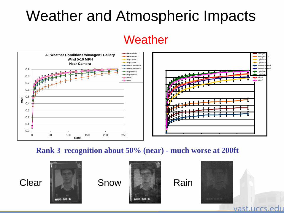
Weather and Atmospheric Impacts
All Weather Conditions w/Image#1 Gallery
Wind 5-10 MPH
Far Camera
0.0
0.1
0.2
0.3
0.4
0.5
0.6
0.7
0.8
0.9
0 50 100 150 200 250Rank
CM
S
HeavyRain-1
HeavyRain-2
LightSnow-1
LightSnow-2
ModerateRain-1
ModerateRain-2
LightRain-1
LightRain-2
Mist-1
Mist-2
All Weather Conditions w/Image#1 Gallery
Wind 5-10 MPH
Near Camera
0.0
0.1
0.2
0.3
0.4
0.5
0.6
0.7
0.8
0.9
0 50 100 150 200 250Rank
CM
S
HeavyRain-1
HeavyRain-2
LightSnow -1
LightSnow -2
ModerateRain-1
ModerateRain-2
LightRain-1
LightRain-2
Mist-1
Mist-2
Rank 3 recognition about 50% (near) - much worse at 200ft
Weather
Clear Snow Rain
3/28/2011 93
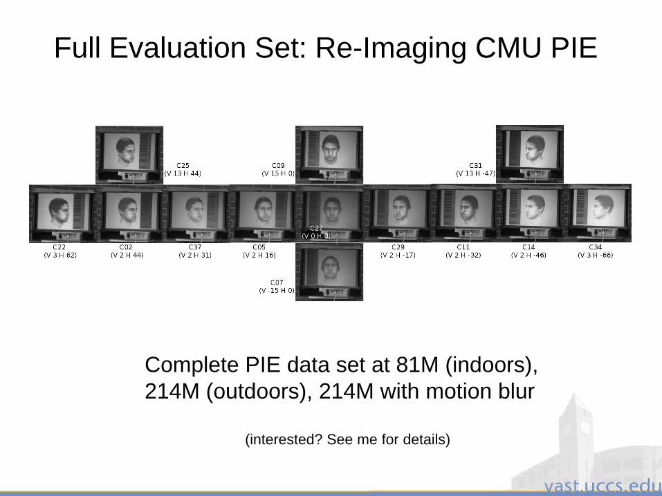
Full Evaluation Set: Re-Imaging CMU PIE
Complete PIE data set at 81M (indoors),
214M (outdoors), 214M with motion blur
(interested? See me for details)
3/28/2011 94
Latest Photo-head Methodology
• Create 3D models from well known 2D Data
– Consider a frontal and profile image
– Establish key points on the face for alignment
• Models allow us to control for pose, and
scene conditions
• Software: Forensica Profiler from Animetrics
– http://www.animetrics.com/products/ForensicaProf
iler.php
3/28/2011 95
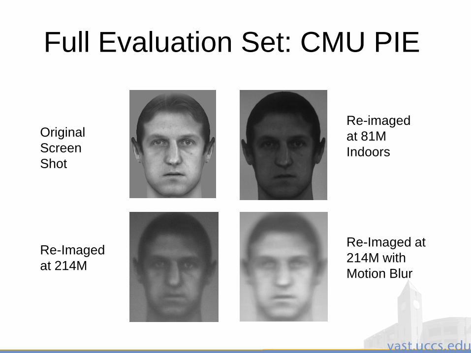
Full Evaluation Set: CMU PIE
Original
Screen
Shot
Re-imaged
at 81M
Indoors
Re-Imaged
at 214M
Re-Imaged at
214M with
Motion Blur
3/28/2011 96
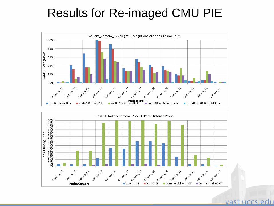
Results for Re-imaged CMU PIE

3/28/2011 97
Illumination Invariance
3/28/2011 98
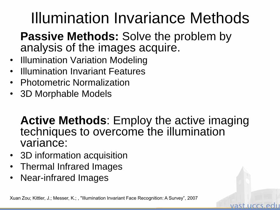
Illumination Invariance MethodsPassive Methods: Solve the problem by analysis of the images acquire.
• Illumination Variation Modeling
• Illumination Invariant Features
• Photometric Normalization
• 3D Morphable Models
Active Methods: Employ the active imaging techniques to overcome the illumination variance:
• 3D information acquisition
• Thermal Infrared Images
• Near-infrared Images
Xuan Zou; Kittler, J.; Messer, K.; , "Illumination Invariant Face Recognition: A Survey”, 2007

3/28/2011 99
Illumination Invariance Methods
Illumination Variation Modeling:
• Linear subspaces, Illumination cone, Generalized photometric Stereo ….
Illumination Invariant Features:
• Direction of Gradient, shape from shading, Quotient Image, EigenPhase, Local Binary Pattern…..
Photometric Normalization:
• Histogram Normalization, Gamma Intensity correction, Local Normalization ….
Xuan Zou; Kittler, J.; Messer, K.; , "Illumination Invariant Face Recognition: A Survey”, 2007

3/28/2011 100
Intensified Image Examples
CSU Standard NormalizationSecurics Dual LUT normalization
Comparison of Normalizations
Raw Normalized
Equinox
Securics
Normalized
CSUNormalizedFrom CVPR04 paper by
Socolinsky & SelingerDual LUT

3/28/2011 101
Advanced Feature Detection
3/28/2011 102
Advanced Feature Detection
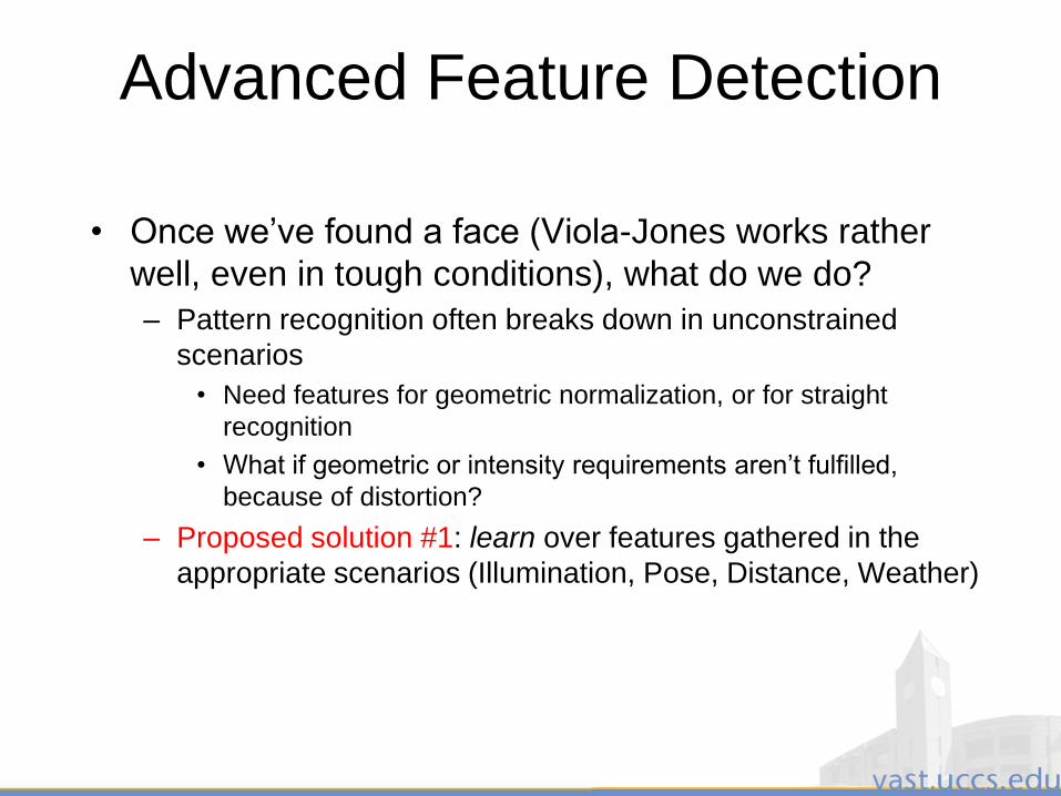
• Once we‟ve found a face (Viola-Jones works rather
well, even in tough conditions), what do we do?
– Pattern recognition often breaks down in unconstrained
scenarios
• Need features for geometric normalization, or for straight
recognition
• What if geometric or intensity requirements aren‟t fulfilled,
because of distortion?
– Proposed solution #1: learn over features gathered in the
appropriate scenarios (Illumination, Pose, Distance, Weather)
3/28/2011 103
Advanced Feature Detection
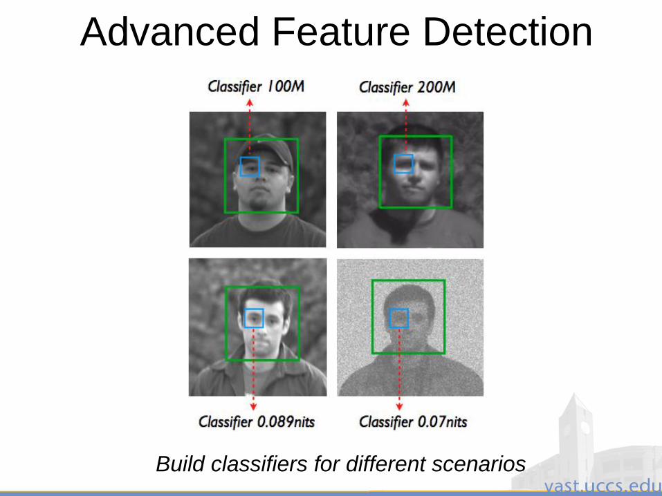
Build classifiers for different scenarios

3/28/2011 104
Advanced Feature Detection
PCA Feature Approach with Machine Learning
3/28/2011 105
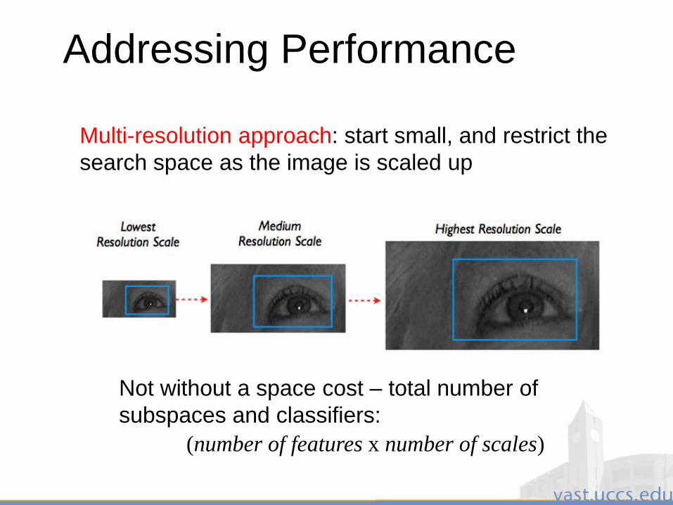
Addressing Performance
Not without a space cost – total number of
subspaces and classifiers:
(number of features x number of scales)
Multi-resolution approach: start small, and restrict the
search space as the image is scaled up
3/28/2011 106
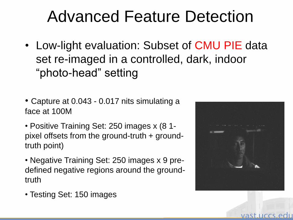
Advanced Feature Detection
• Low-light evaluation: Subset of CMU PIE data
set re-imaged in a controlled, dark, indoor
“photo-head” setting
• Capture at 0.043 - 0.017 nits simulating a
face at 100M
• Positive Training Set: 250 images x (8 1-
pixel offsets from the ground-truth + ground-
truth point)
• Negative Training Set: 250 images x 9 pre-
defined negative regions around the ground-
truth
• Testing Set: 150 images
3/28/2011 107
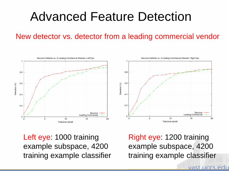
Advanced Feature Detection
New detector vs. detector from a leading commercial vendor
Left eye: 1000 training
example subspace, 4200
training example classifier
Right eye: 1200 training
example subspace, 4200
training example classifier

3/28/2011 108
Advanced Feature Detection
Left:
Learning
Based
Detector
Right: A
Leading
Commercial
Detector
No Eyes Found
Qualitative Results
3/28/2011 109
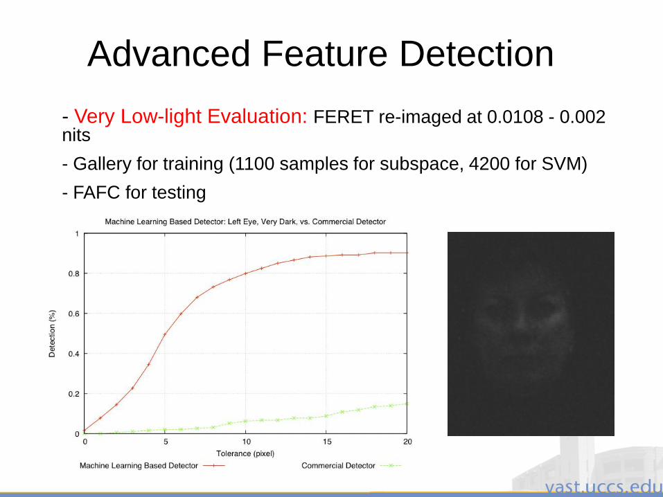
Advanced Feature Detection
- Very Low-light Evaluation: FERET re-imaged at 0.0108 - 0.002 nits
- Gallery for training (1100 samples for subspace, 4200 for SVM)
- FAFC for testing

3/28/2011 110
Advanced Feature Detection
- Blur Evaluation: FERET ba, bj, bk subsets
- 3 blur models for testing: 15 pixels - 122º,
17 pixels - 59º, 20 pixels - 62º
- SVM Trained on
2,000 base images
using the 20 pixels, 52º
model
- Subspace trained on
1,000 images from the
same model
- Tested on 150 images
with various levels of
blur
3/28/2011 111
Advanced Feature Detection
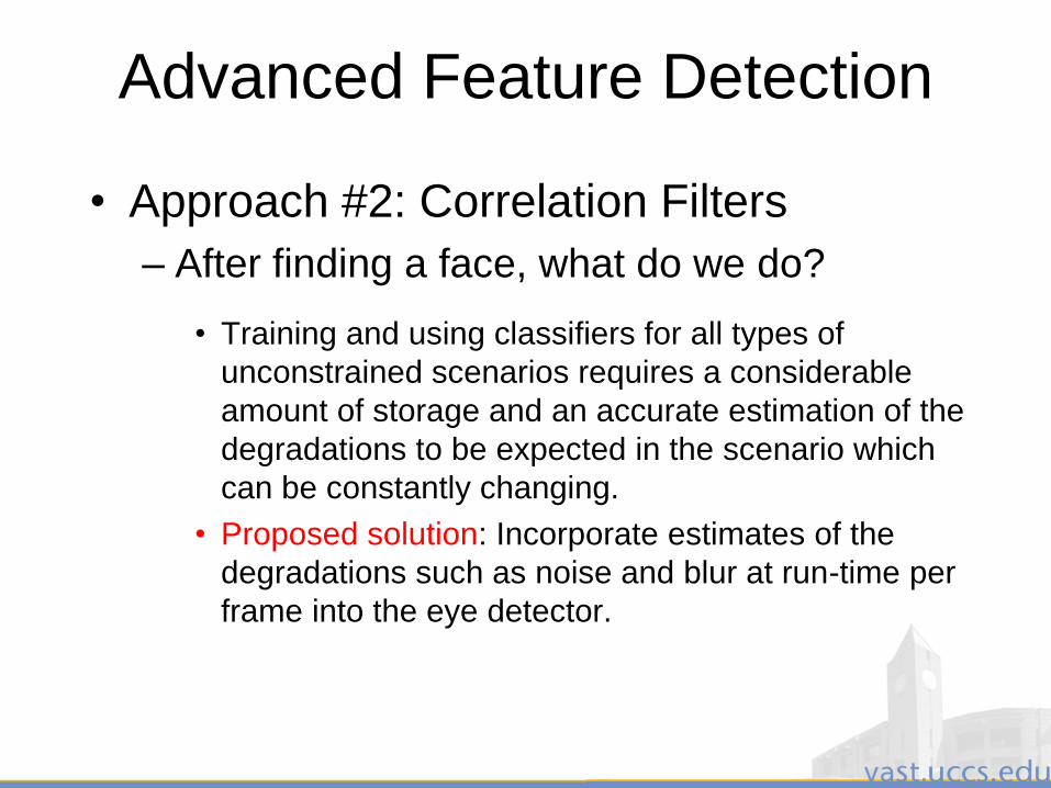
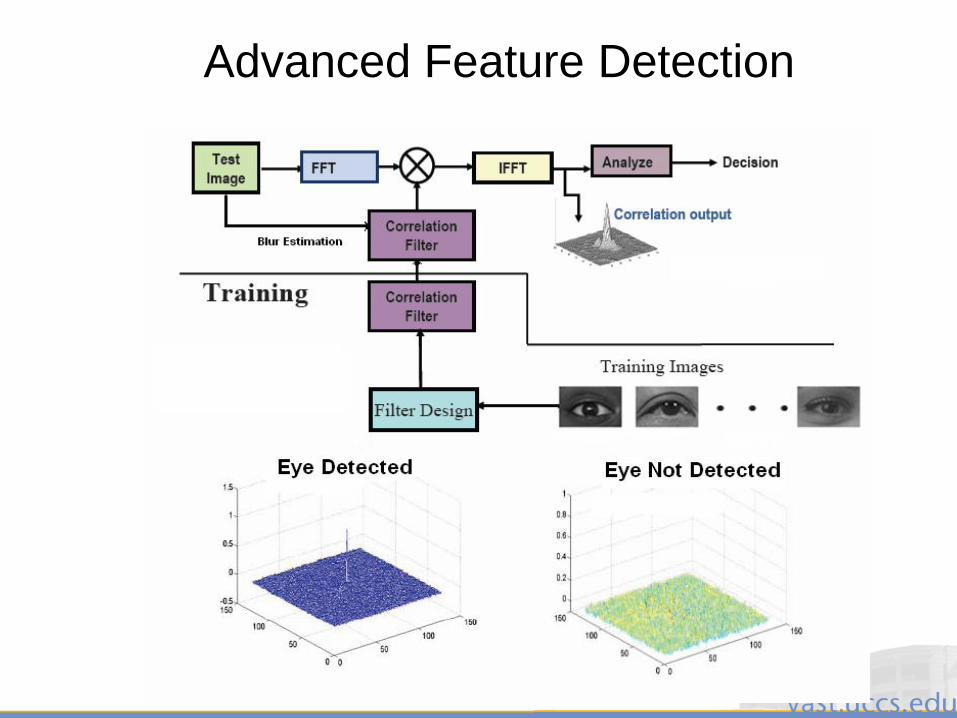
• Approach #2: Correlation Filters
– After finding a face, what do we do?
• Training and using classifiers for all types of
unconstrained scenarios requires a considerable
amount of storage and an accurate estimation of the
degradations to be expected in the scenario which
can be constantly changing.
• Proposed solution: Incorporate estimates of the
degradations such as noise and blur at run-time per
frame into the eye detector.
3/28/2011 112
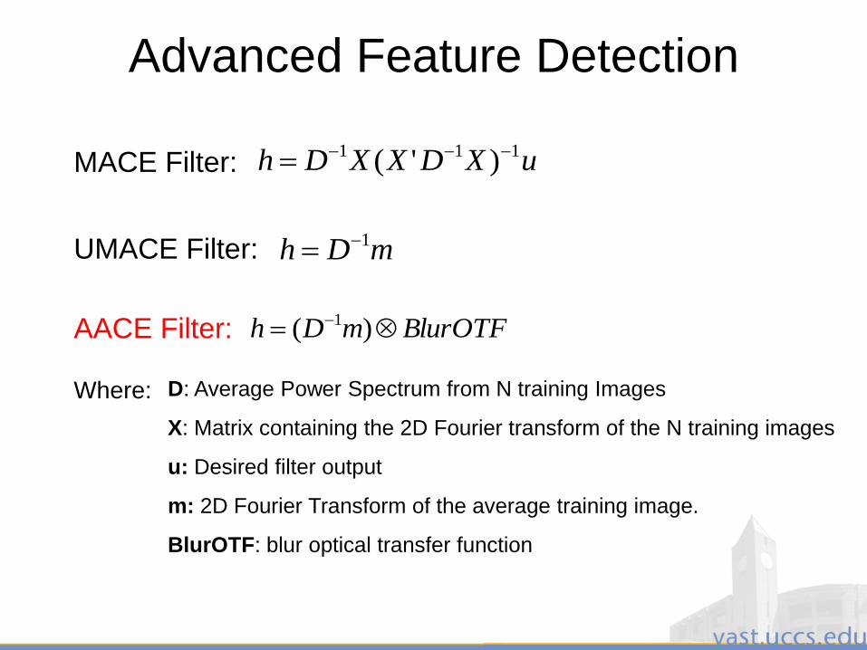
Advanced Feature Detection
uXDXXDh 111 )'(
mDh 1
BlurOTFmDh )( 1
MACE Filter:
UMACE Filter:
AACE Filter:
Where: D: Average Power Spectrum from N training Images
X: Matrix containing the 2D Fourier transform of the N training images
u: Desired filter output
m: 2D Fourier Transform of the average training image.
BlurOTF: blur optical transfer function
3/28/2011 113
Advanced Feature Detection

3/28/2011 114
Advanced Feature Detection
Correlation based detector vs. detector from a leading
commercial vendor
Left and Right eyeMACE filter: 6 training imgs. AACE filter: 266 training imgs.

3/28/2011 115
Advanced Feature Detection
- Very Low-light Evaluation: FERET re-imaged at 0.0108 - 0.002 nits
- MACE Filter: 4 Training Images
- AACE Filter: 588 Training Images
- FAFC for testing
3/28/2011 116
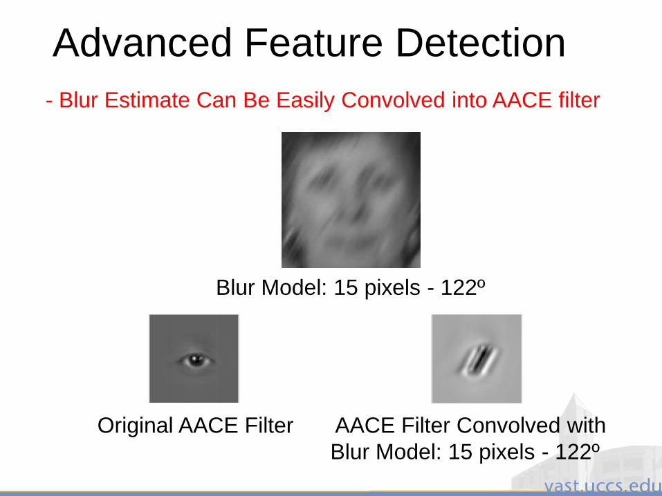
Advanced Feature Detection
- Blur Estimate Can Be Easily Convolved into AACE filter
AACE Filter Convolved with
Blur Model: 15 pixels - 122º
Original AACE Filter
Blur Model: 15 pixels - 122º

3/28/2011 117
Advanced Feature Detection- Blur Evaluation: FERET ba, bj, bk subsets
- 3 blur models for testing: 15 pixels - 122º,
17 pixels - 59º, 20 pixels - 62º
- AACE filter trained on
1,500 original images
then convolved with the
20 pixels, 52º model
- Tested on 150 images
with various levels of blur

3/28/2011 118
Mitigating the Effects of Blur
3/28/2011 119
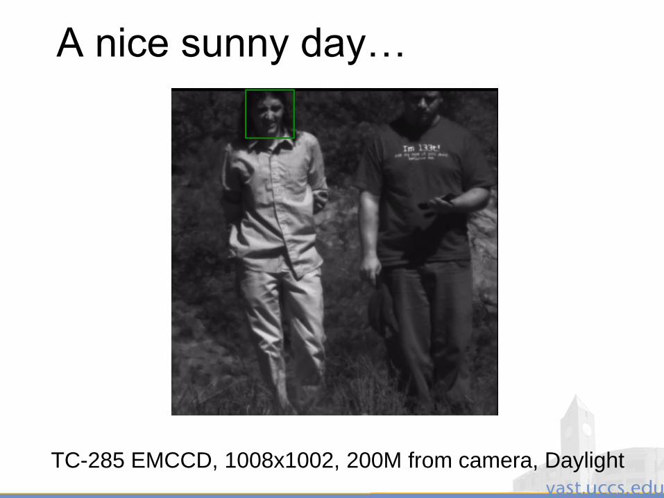
A nice sunny day…
TC-285 EMCCD, 1008x1002, 200M from camera, Daylight
3/28/2011 120
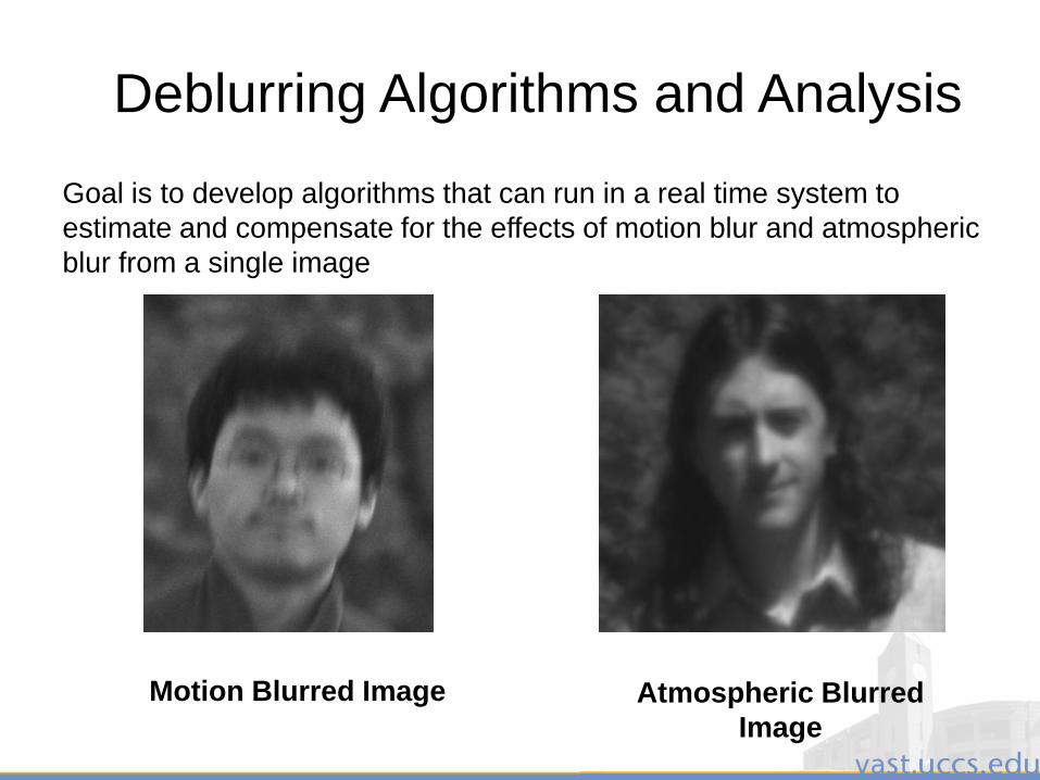
Goal is to develop algorithms that can run in a real time system to
estimate and compensate for the effects of motion blur and atmospheric
blur from a single image
Atmospheric Blurred
Image
Deblurring Algorithms and Analysis
Motion Blurred Image
3/28/2011 121
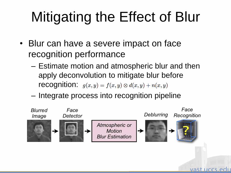
Mitigating the Effect of Blur
• Blur can have a severe impact on face
recognition performance
– Estimate motion and atmospheric blur and then
apply deconvolution to mitigate blur before
recognition:
– Integrate process into recognition pipeline

3/28/2011 122
Mitigating the Effect of Blur
• Motion blur estimation
– Use the Cepstrum of the image to identify blur
angle and length
(a) Original
image
(b) Cepstrum of
original image
(c) Motion
blur at 45˚
(d) Cepstrum of motion
blurred image reflecting
blur angle

3/28/2011 123
Mitigating the Effect of Blur
• Image restoration for motion blur
– CLS filter helps eliminate oscillations in
output image
controls low-pass filtering; P(u,v) is the Fourier
transform of the smoothness criterion function
3/28/2011 124
Mitigating the Effect of Blur
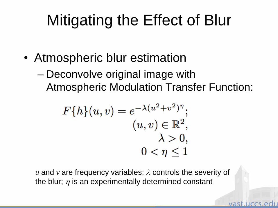
• Atmospheric blur estimation
– Deconvolve original image with
Atmospheric Modulation Transfer Function:
u and v are frequency variables; controls the severity of
the blur; is an experimentally determined constant
3/28/2011 125
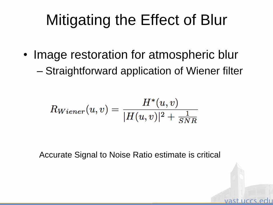
Mitigating the Effect of Blur
• Image restoration for atmospheric blur
– Straightforward application of Wiener filter
Accurate Signal to Noise Ratio estimate is critical
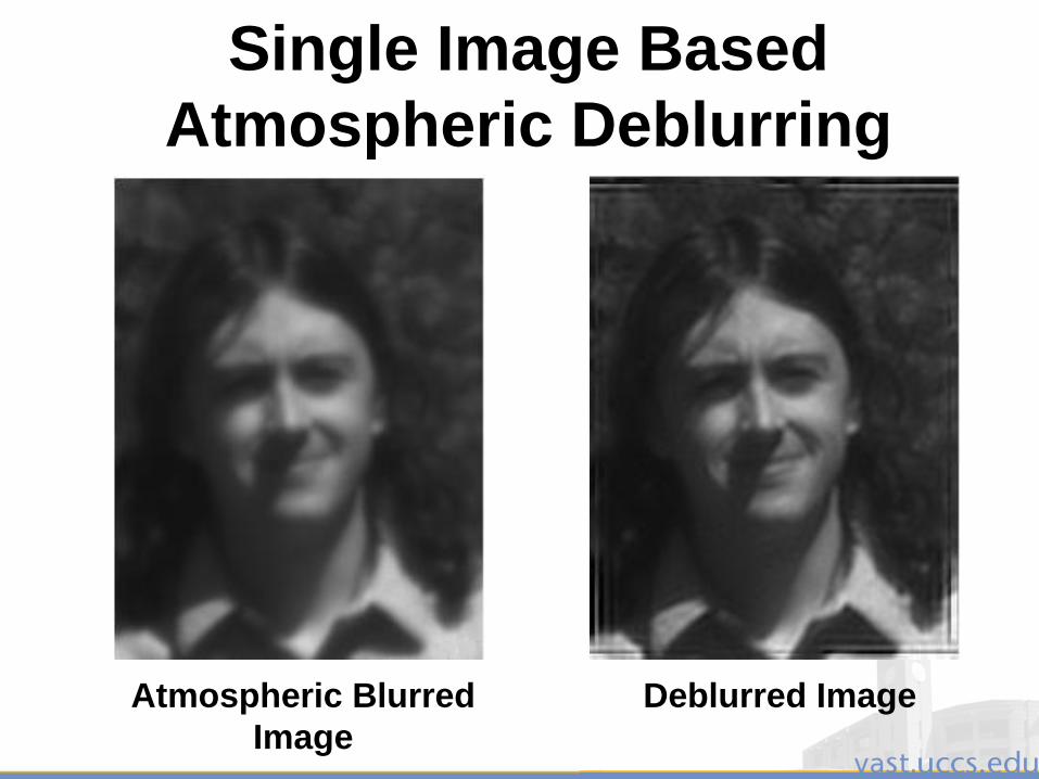
3/28/2011 126
Atmospheric Blurred
Image
Deblurred Image
Single Image Based
Atmospheric Deblurring
3/28/2011 127
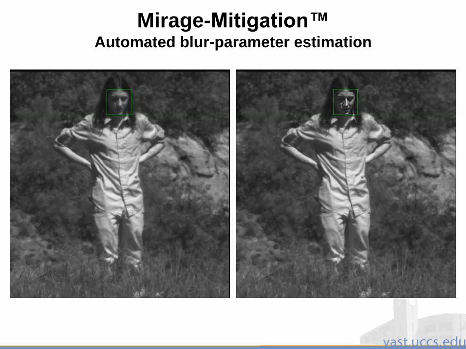
Mirage-Mitigation™Automated blur-parameter estimation

3/28/2011 128
Single Image SNR Estimation
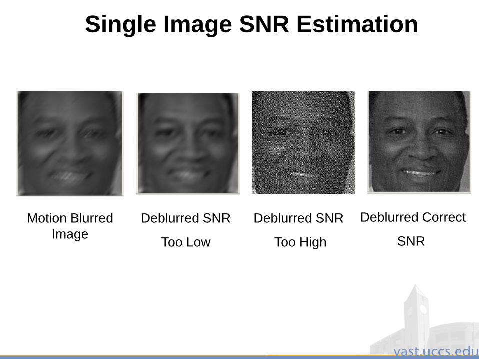
3/28/2011 129
Single Image SNR Estimation
Motion Blurred
Image
Deblurred SNR
Too Low
Deblurred SNR
Too High
Deblurred Correct
SNR

3/28/2011 130
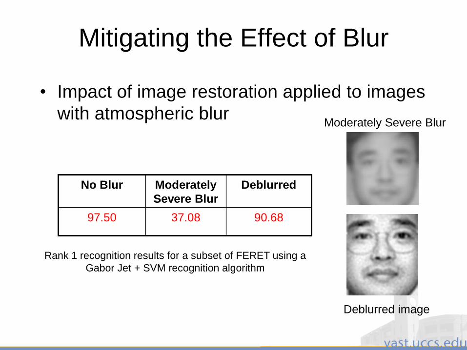
Mitigating the Effect of Blur
• Impact of image restoration applied to images
with motion blur
Blur None 10px 15px 20px
Baseline blurred 97.50 75.00 39.58 16.67
Deblurred - 92.89 93.75 86.67
Rank 1 recognition results for a subset of FERET using a
Gabor Jet + SVM recognition algorithm
10 pixel blur
Deblurred image
3/28/2011 131
Mitigating the Effect of Blur
• Impact of image restoration applied to images
with atmospheric blur
No Blur Moderately
Severe Blur
Deblurred
97.50 37.08 90.68
Rank 1 recognition results for a subset of FERET using a
Gabor Jet + SVM recognition algorithm
Moderately Severe Blur
Deblurred image
3/28/2011 132
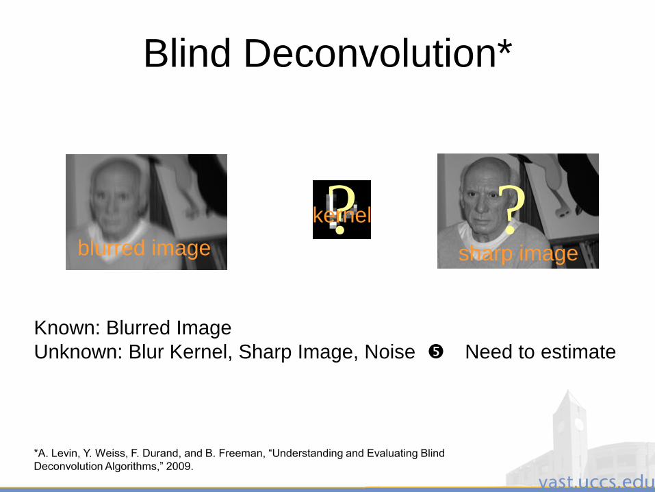
Blind Deconvolution*
blurred image
??kernel
sharp image
*A. Levin, Y. Weiss, F. Durand, and B. Freeman, “Understanding and Evaluating Blind
Deconvolution Algorithms,” 2009.
Known: Blurred Image
Unknown: Blur Kernel, Sharp Image, Noise Need to estimate

3/28/2011 133
Naïve MAPx,k estimation
log p(x,k | y) 1
2| k x y |2 xii
, 1
Find a kernel k and latent image x minimizing:
Should favor sharper x explanations
Convolution
constraint
Sparse prior
3/28/2011 134
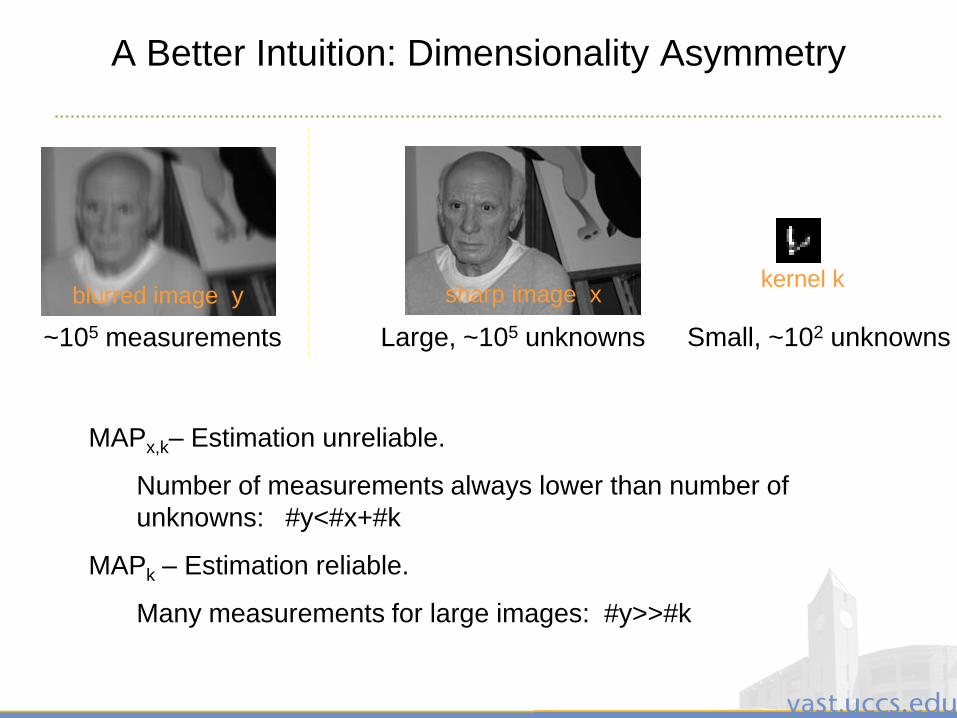
A Better Intuition: Dimensionality Asymmetry
Large, ~105 unknowns Small, ~102 unknowns
blurred image ykernel k
sharp image x
~105 measurements
MAPx,k– Estimation unreliable.
Number of measurements always lower than number of
unknowns: #y<#x+#k
MAPk – Estimation reliable.
Many measurements for large images: #y>>#k
3/28/2011 135
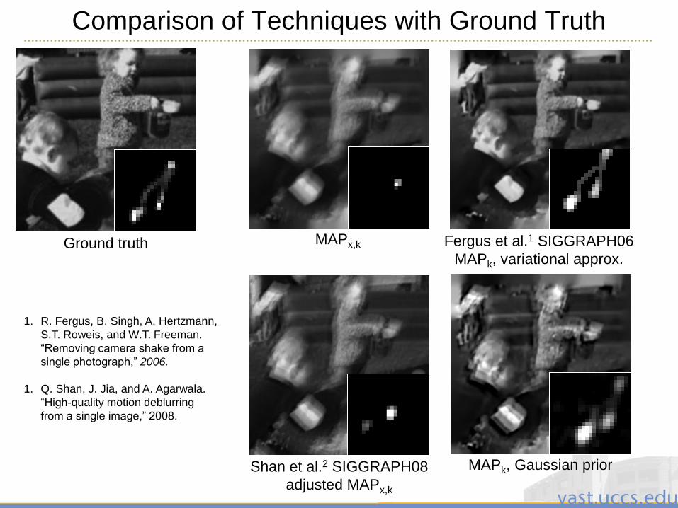
Comparison of Techniques with Ground Truth
Fergus et al.1 SIGGRAPH06
MAPk, variational approx.
Shan et al.2 SIGGRAPH08
adjusted MAPx,k
MAPx,k
MAPk, Gaussian prior
Ground truth
1. R. Fergus, B. Singh, A. Hertzmann,
S.T. Roweis, and W.T. Freeman.
“Removing camera shake from a
single photograph,” 2006.
1. Q. Shan, J. Jia, and A. Agarwala.
“High-quality motion deblurring
from a single image,” 2008.

3/28/2011 136
Applicability to Face Recognition
Fergus et al.1 SIGGRAPH06
MAPk, variational approx.
What is visually appealing may not work very
well for recognition.
Evaluation for face recognition?
3/28/2011 137
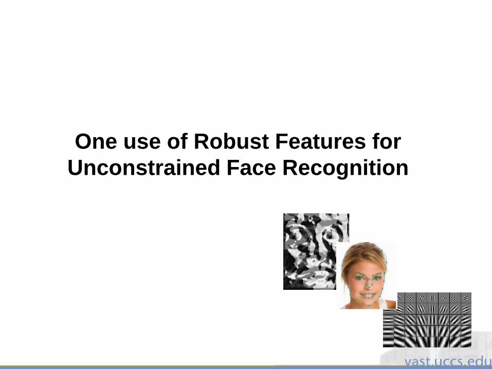
One use of Robust Features for
Unconstrained Face Recognition
3/28/2011 138
Non-Cooperative Face Recognition Methods
• Features Based Recognition
• 3D Approaches
• Video Based Face Recognition
• Pose and Occlusion Invariant Methods
• Biologically Inspired Methods
3/28/2011 139
Features Used in Face Recognition
• PCA/LDA/ICA
• GABOR
• LBP
• SIFT
• Edges/Regions
3/28/2011 140
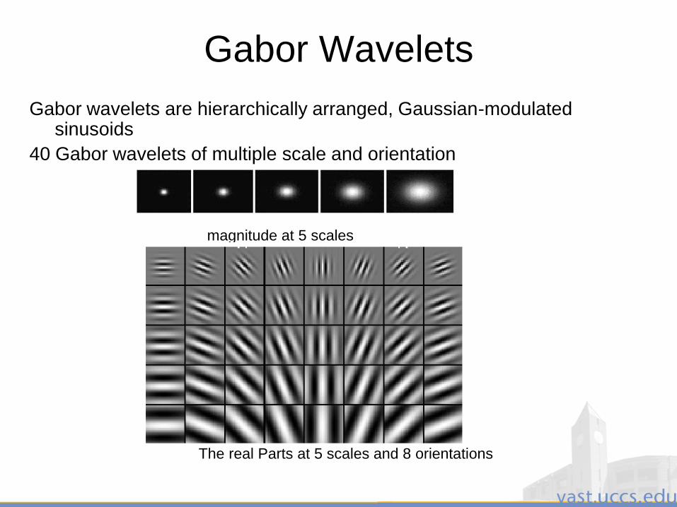
Gabor Wavelets
Gabor wavelets are hierarchically arranged, Gaussian-modulated sinusoids
40 Gabor wavelets of multiple scale and orientation
magnitude at 5 scales
The real Parts at 5 scales and 8 orientations
3/28/2011 141
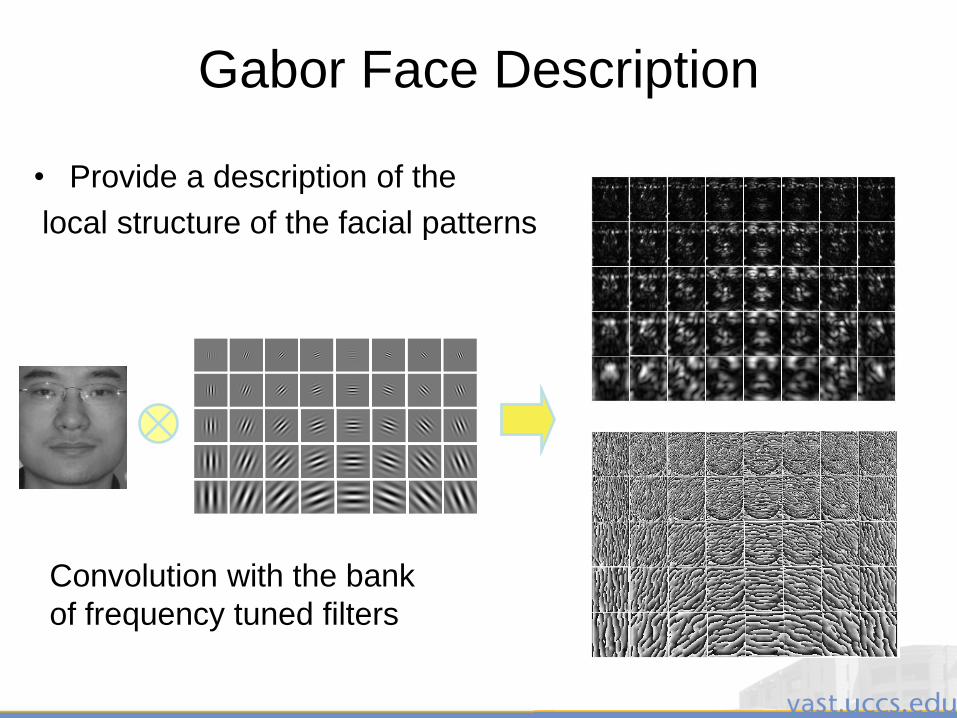
Gabor Face Description
• Provide a description of the
local structure of the facial patterns
Convolution with the bank
of frequency tuned filters

3/28/2011 142
Gabor: Analytical Methods
• Graph Based methods:- Elastic Bunch Graph Matching (EGBM)
- Face Bunch Graphs
- Dynamic Link Architecture (DLA)
• Non-Graph Based Methods:- Manual Extraction of feature points
- Color based extraction
- Ridge/valley/Edge based feature points extraction
- Gaussian mixture model
- Non-Uniform sampling
*Angel Serrano, Isaac Martin de Diego, Cristina Conde, Enrique Cabello, Recent advances in face biometrics with Gabor
wavelets: A review,2010)
3/28/2011 143
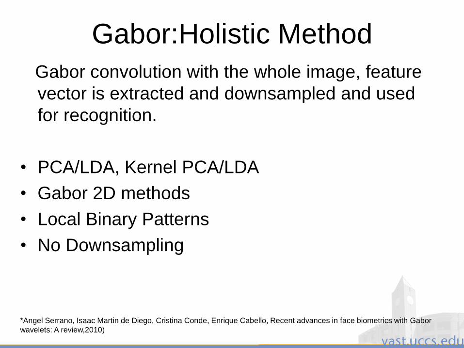
Gabor:Holistic Method
Gabor convolution with the whole image, feature
vector is extracted and downsampled and used
for recognition.
• PCA/LDA, Kernel PCA/LDA
• Gabor 2D methods
• Local Binary Patterns
• No Downsampling
*Angel Serrano, Isaac Martin de Diego, Cristina Conde, Enrique Cabello, Recent advances in face biometrics with Gabor
wavelets: A review,2010)
3/28/2011 144
Motivation behind Gabor Wavelets
in face recognition
• Biological Motivation: Images in primary visual cortex (V1) are represented in terms of Gabor wavelets. The shapes of Gabor Wavelets are similar to the receptive fields of simple cells in the primary visual cortex.
• Mathematical Motivation: The Gabor wavelets are optimal for measuring local spatial frequencies.
• Empirical Motivation: They have been successfully used for distortion, scale and rotation invariant pattern recognition tasks such as handwritten, texture and
fingerprint recognition.
*Linlin Shen, Li Bai, A review on Gabor wavelets for face recognition, 2006
3/28/2011 145
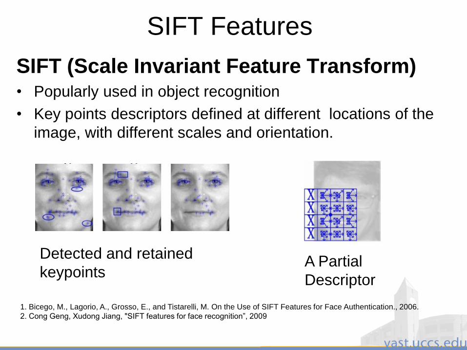
SIFT Features
SIFT (Scale Invariant Feature Transform)• Popularly used in object recognition
• Key points descriptors defined at different locations of the
image, with different scales and orientation.
1. Bicego, M., Lagorio, A., Grosso, E., and Tistarelli, M. On the Use of SIFT Features for Face Authentication., 2006.
2. Cong Geng, Xudong Jiang, "SIFT features for face recognition”, 2009
Detected and retained
keypointsA Partial
Descriptor
3/28/2011 146
Findings from SIFT in Face Recognition
• Not very well suited for face recognition because
of complexity, non-planarity and self-occlusion
found in the face recognition problem.
• Some modifications in the original SIFT
algorithms to be adopted in face recognition:
Keypoint-Preserving-SIFT, Partial-Descriptor
Keypoint, person-specific matching algorithms
etc.
3/28/2011 147
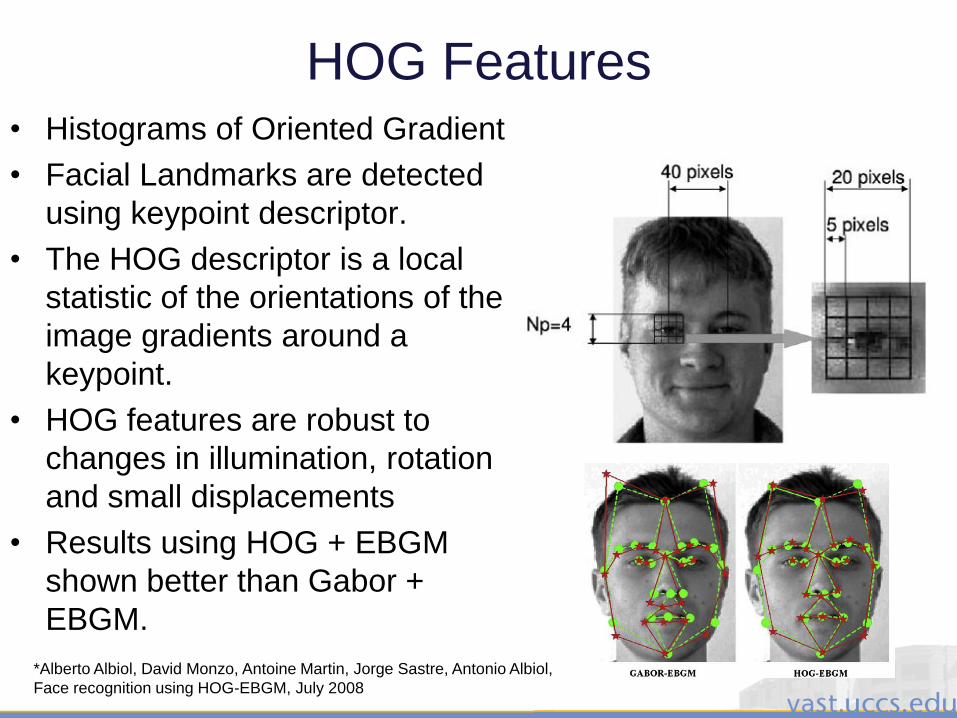
HOG Features• Histograms of Oriented Gradient
• Facial Landmarks are detected
using keypoint descriptor.
• The HOG descriptor is a local
statistic of the orientations of the
image gradients around a
keypoint.
• HOG features are robust to
changes in illumination, rotation
and small displacements
• Results using HOG + EBGM
shown better than Gabor +
EBGM.
*Alberto Albiol, David Monzo, Antoine Martin, Jorge Sastre, Antonio Albiol,
Face recognition using HOG-EBGM, July 2008
3/28/2011 148
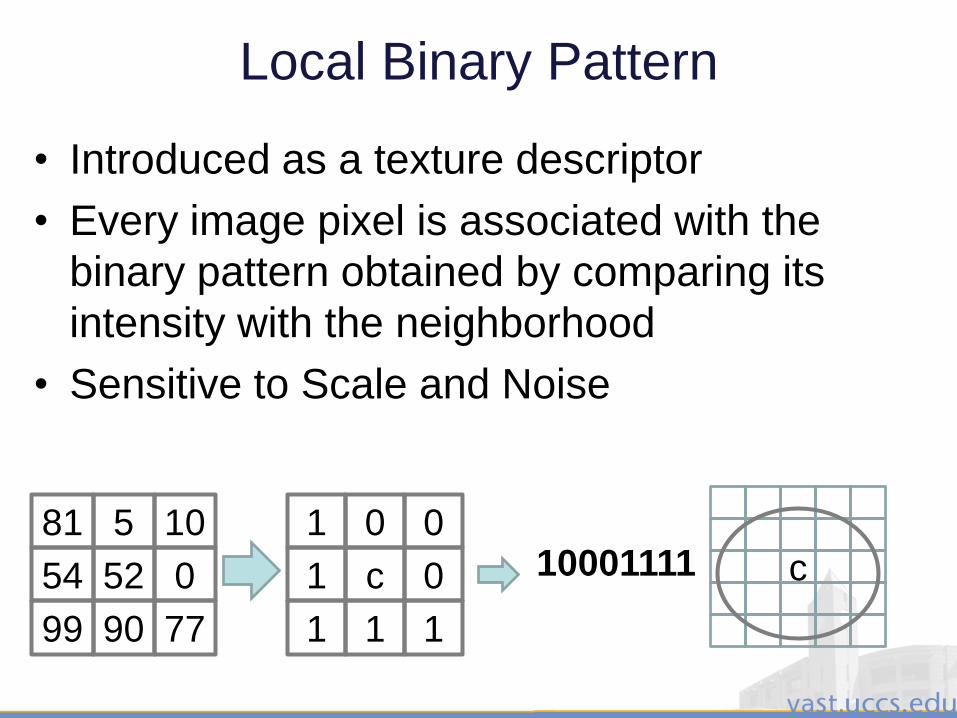
Local Binary Pattern
• Introduced as a texture descriptor
• Every image pixel is associated with the
binary pattern obtained by comparing its
intensity with the neighborhood
• Sensitive to Scale and Noise
81
54
10
99 90
0
5
77
52
1
1
0
1 1
0
0
1
c 10001111 c
3/28/2011 149
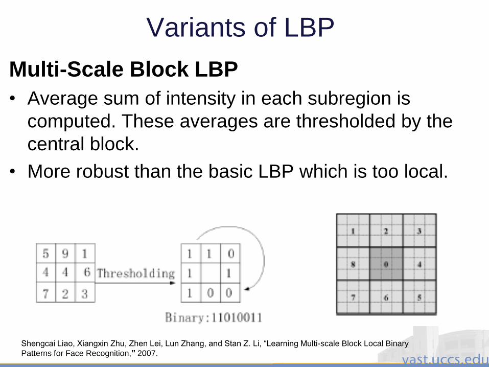
Variants of LBP
Multi-Scale Block LBP
• Average sum of intensity in each subregion is
computed. These averages are thresholded by the
central block.
• More robust than the basic LBP which is too local.
Shengcai Liao, Xiangxin Zhu, Zhen Lei, Lun Zhang, and Stan Z. Li, “Learning Multi-scale Block Local Binary
Patterns for Face Recognition,” 2007.
3/28/2011 150
Variants of LBP
• Local Ternary Pattern: 3-valued coding
that includes a threshold around zero for
improved resistance to noise
*Xiaoyang Tan; Triggs, B.; , "Enhanced Local Texture Feature Sets for Face Recognition Under
Difficult Lighting Conditions”
3/28/2011 151
LBP on Gabor Magnitude map
• Each normalized images is converted into Gabor Magnitude map by
convolving with Gabor filters.
• Local Binary Pattern Map of each GMP is generated and features are
extracted and concatenated.
*Wenchao Zhang; Shiguang Shan; Wen Gao; Xilin Chen; Hongming Zhang; , "Local Gabor binary pattern histogram
sequence (LGBPHS): a novel non-statistical model for face representation and recognition
3/28/2011 152
GRAB Operator General Region Assigned to BinaryA representation of GRAB-N
• Each NxN region computes the a measure (e.g. average intensity) in that region
• If the central measure is significantly different than measure for neighbor k, then set bit k to 1, else set to 0
• This model allows to incorporate changes in resolutions/scale, as well as camera noise.
Normalized
Image
Smoothed
Image
computed
using Integral
image.
Grabbed
Image
A. Sapkota, B. Parks, W. Scheirer, and T. Boult, “FACE-GRAB: Face
Recognition with General Region Assigned to Binary Operator,” 2010

3/28/2011 153
GRAB Operator
1
0
0 0
111
110001111
92
5
32 12
180105128
97 85
GRAB-3 Example
3/28/2011 154
GRABBed Images
LBP and the lower windowed GRAB images are
impacted by noise and low resolution artifacts.
Higher GRAB windows have balance between
texture information and noise.
Geo-
Normalized
Image
LB
P
GRA
B-3
GRA
B-5
GRA
B-9GRA
B-7
3/28/2011 155
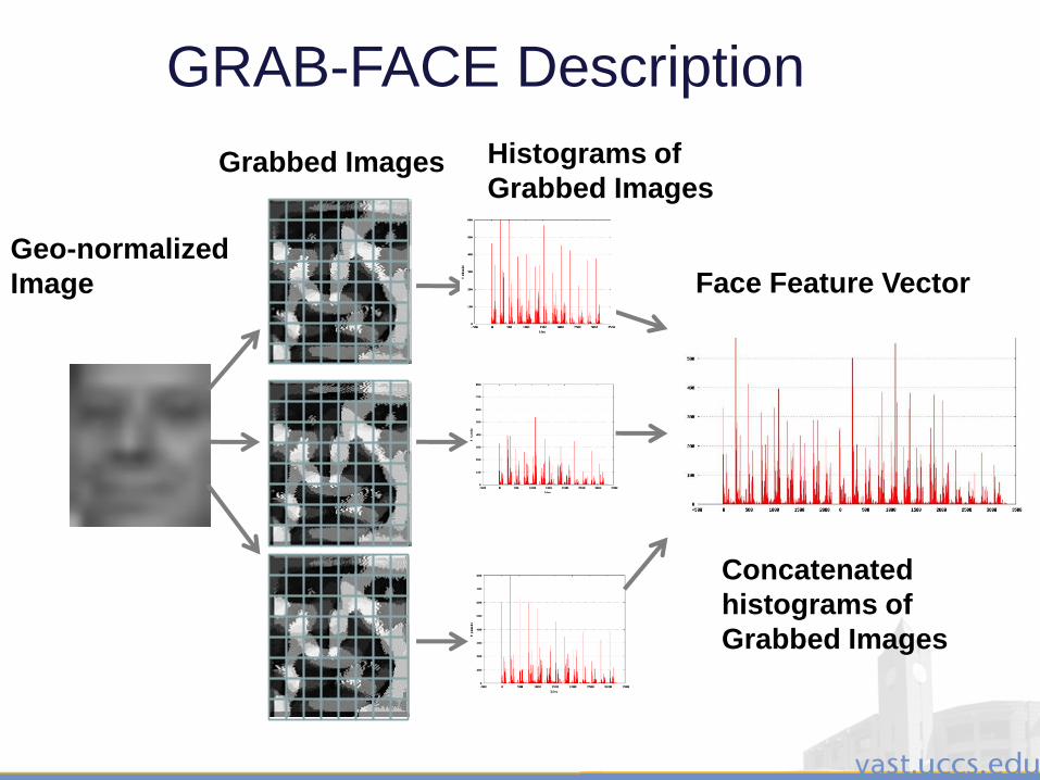
GRAB-FACE Description
Geo-normalized
Image
Grabbed Images
Face Feature Vector
Histograms of
Grabbed Images
Concatenated
histograms of
Grabbed Images
3/28/2011 156
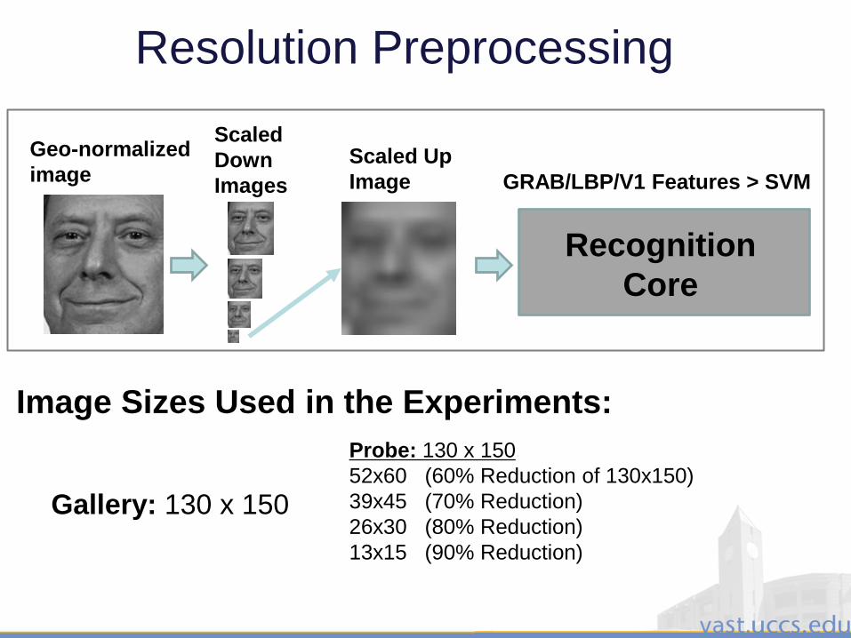
Resolution Preprocessing
Geo-normalized
image
Scaled
Down
Images
Scaled Up
Image
Probe: 130 x 150
52x60 (60% Reduction of 130x150)
39x45 (70% Reduction)
26x30 (80% Reduction)
13x15 (90% Reduction)
Image Sizes Used in the Experiments:
Gallery: 130 x 150
Recognition
Core
GRAB/LBP/V1 Features > SVM

3/28/2011 157
Classification Method
• Support Vector Machine (SVM) was used
• Performance Gain using SVM compared to Nearest-Neighbor
• Results of LBP was verified using standard FERET protocol using Nearest Neighbor Classification
• PCA is important for Gabor features but did not help GRAB and LBP.
LBP
Histograms
GRAB
Histograms
Gabor
Features
PCA (Optional) SVM
3/28/2011 158
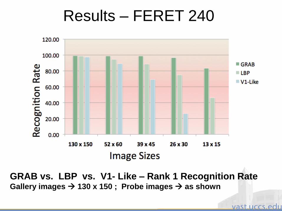
Results – FERET 240
GRAB vs. LBP vs. V1- Like – Rank 1 Recognition Rate Gallery images 130 x 150 ; Probe images as shown
3/28/2011 159
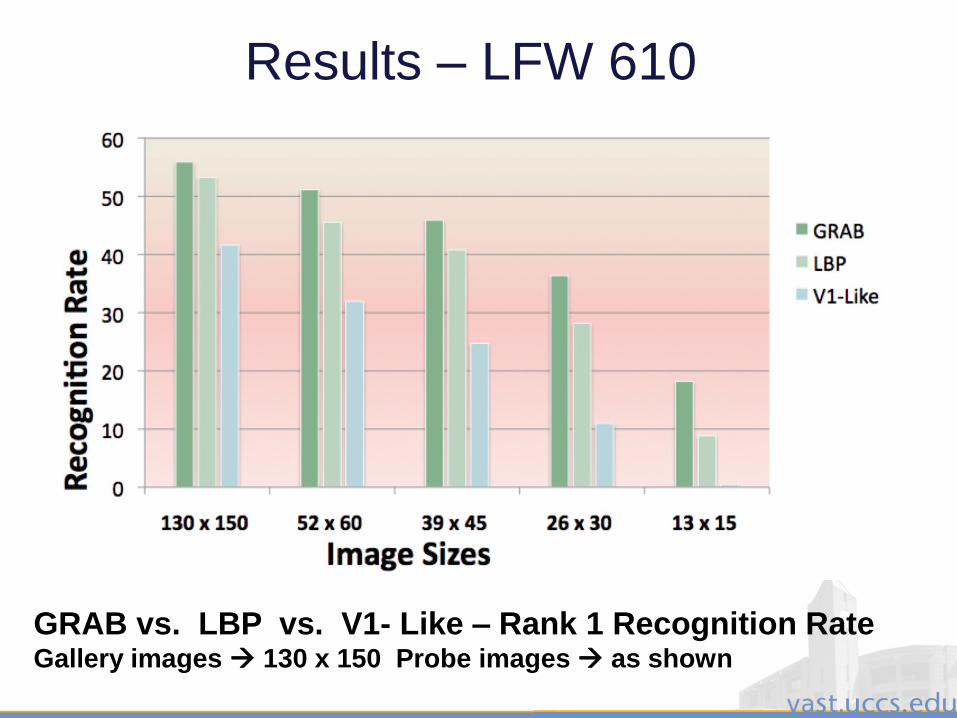
GRAB vs. LBP vs. V1- Like – Rank 1 Recognition RateGallery images 130 x 150 Probe images as shown
Results – LFW 610
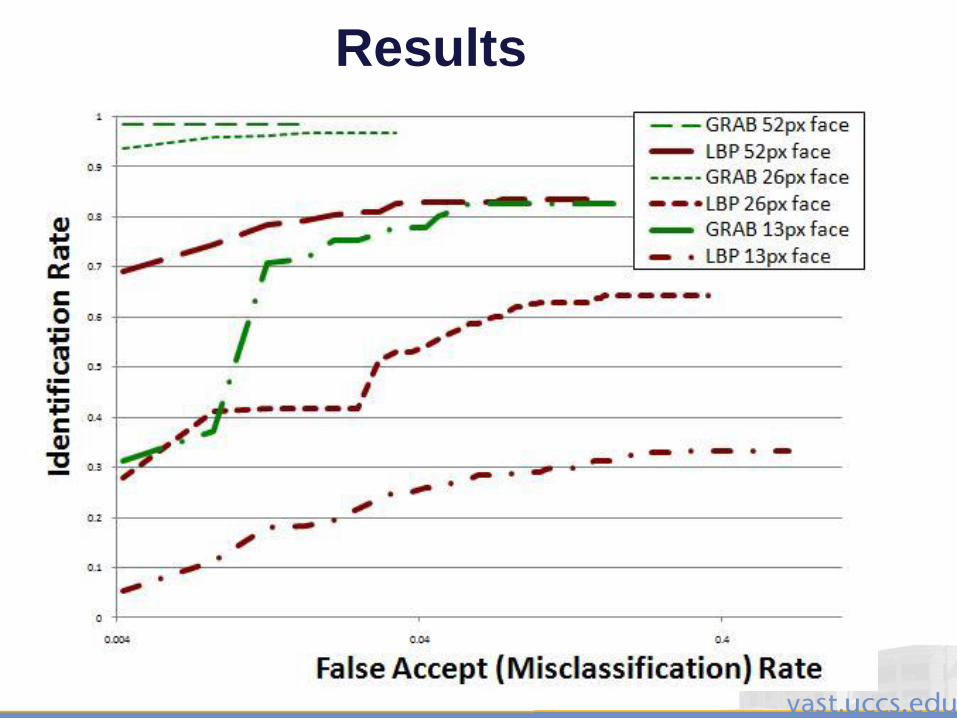
3/28/2011 160
Results

3/28/2011 161
How well can a face be
represented using such
features?
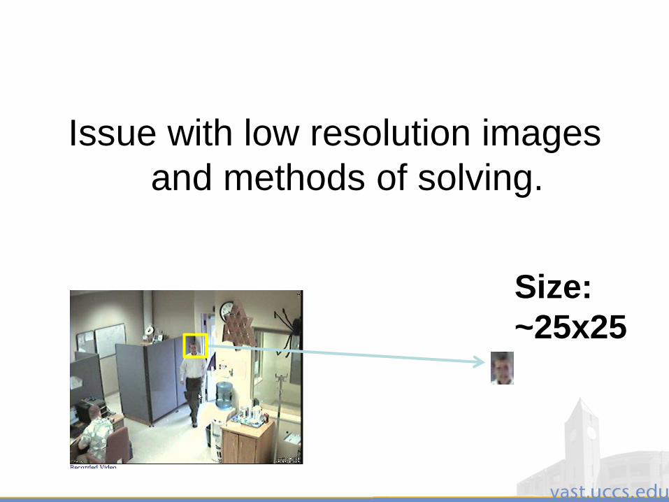
3/28/2011 162
Issue with low resolution images
and methods of solving.
Size:
~25x25
3/28/2011 163
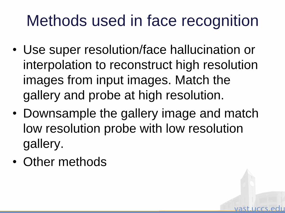
Methods used in face recognition
• Use super resolution/face hallucination or
interpolation to reconstruct high resolution
images from input images. Match the
gallery and probe at high resolution.
• Downsample the gallery image and match
low resolution probe with low resolution
gallery.
• Other methods

3/28/2011 164
Super Resolution/Hallucinating Faces
• Super-Resolution reconstruction produces one or a set of
high-resolution images from one or a sequence of low-
resolution frames.
• Depending upon the requirement the
following techniques are available.
- Input output
- Singe LR image single HR image
- Multiple LR frames single HR image
- Multiple LR frames sequence of HR images
3/28/2011 165
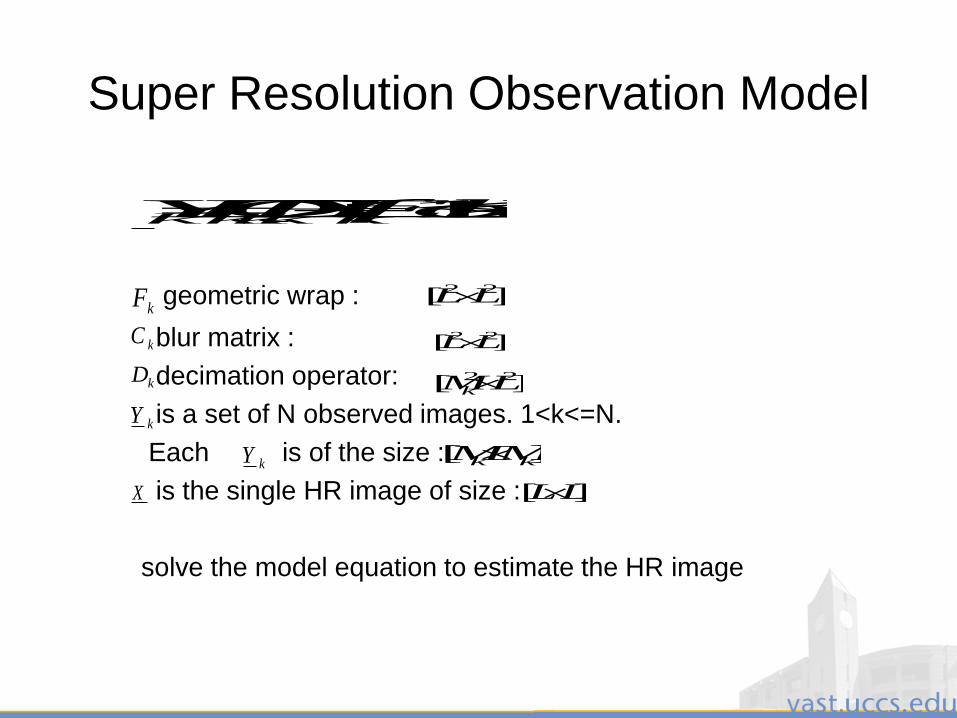
Super Resolution Observation Model
geometric wrap :
blur matrix :
decimation operator:
is a set of N observed images. 1<k<=N.
Each is of the size :
is the single HR image of size :
solve the model equation to estimate the HR image
NkforEXFCDY kkkkk 1
kF
kC
kD
][ 22 LL
][ 22 LL
][ 22 LMk
kY
kY
][ kk MM
][ LLX
3/28/2011 166
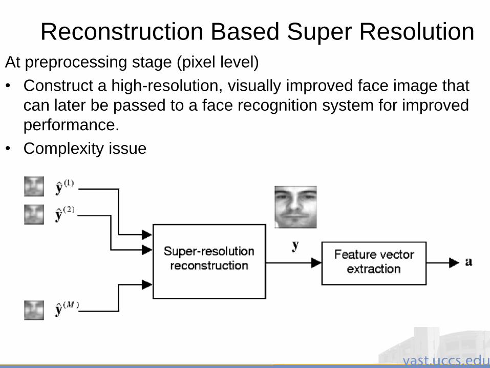
Reconstruction Based Super ResolutionAt preprocessing stage (pixel level)
• Construct a high-resolution, visually improved face image that
can later be passed to a face recognition system for improved
performance.
• Complexity issue
3/28/2011 167
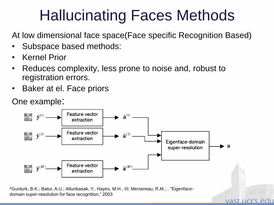
Hallucinating Faces MethodsAt low dimensional face space(Face specific Recognition Based)
• Subspace based methods:
• Kernel Prior
• Reduces complexity, less prone to noise and, robust to registration errors.
• Baker at el. Face priors
One example:
*Gunturk, B.K.; Batur, A.U.; Altunbasak, Y.; Hayes, M.H., III; Mersereau, R.M.; , "Eigenface-
domain super-resolution for face recognition,” 2003
3/28/2011 168
Face Super Resolution Methods
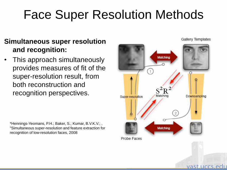
Simultaneous super resolution
and recognition:
• This approach simultaneously
provides measures of fit of the
super-resolution result, from
both reconstruction and
recognition perspectives.
*Hennings-Yeomans, P.H.; Baker, S.; Kumar, B.V.K.V.; ,
"Simultaneous super-resolution and feature extraction for
recognition of low-resolution faces, 2008
3/28/2011 169
Face Super Resolution Methods
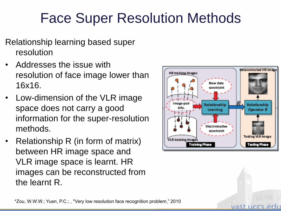
Relationship learning based super
resolution
• Addresses the issue with
resolution of face image lower than
16x16.
• Low-dimension of the VLR image
space does not carry a good
information for the super-resolution
methods.
• Relationship R (in form of matrix)
between HR image space and
VLR image space is learnt. HR
images can be reconstructed from
the learnt R.
*Zou, W.W.W.; Yuen, P.C.; , "Very low resolution face recognition problem,” 2010
3/28/2011 170
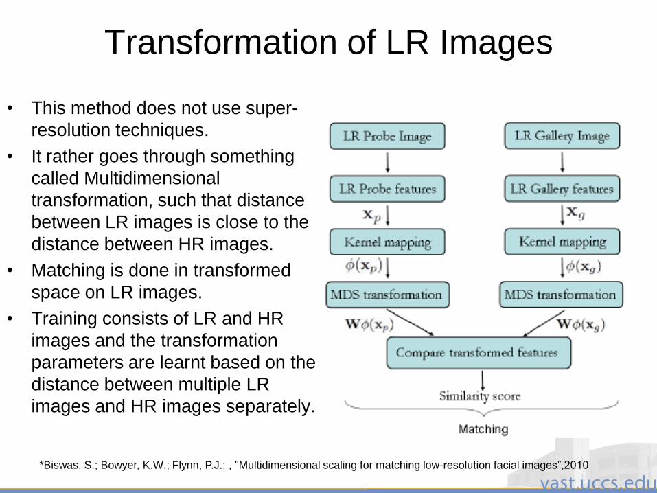
Transformation of LR Images
• This method does not use super-
resolution techniques.
• It rather goes through something
called Multidimensional
transformation, such that distance
between LR images is close to the
distance between HR images.
• Matching is done in transformed
space on LR images.
• Training consists of LR and HR
images and the transformation
parameters are learnt based on the
distance between multiple LR
images and HR images separately.
*Biswas, S.; Bowyer, K.W.; Flynn, P.J.; , "Multidimensional scaling for matching low-resolution facial images”,2010

3/28/2011 171
Face Super Resolution Methods• Reconstruction of SR face images using multiple occluded
images of different resolutions which are commonly
encountered in surveillance videos.
• Performs hierarchical patch-wise alignment and global
Bayesian inference.
• Considers the spatial constraints and exploit the inter-frame
constraints across multiple face images of different
resolutions
Low Resolution
Images
Resulting
Image
Ground
Truth
*K. Jia, S. Gong, Face super-resolution
using multiple occluded images of
different resolutions, 2005
3/28/2011 172
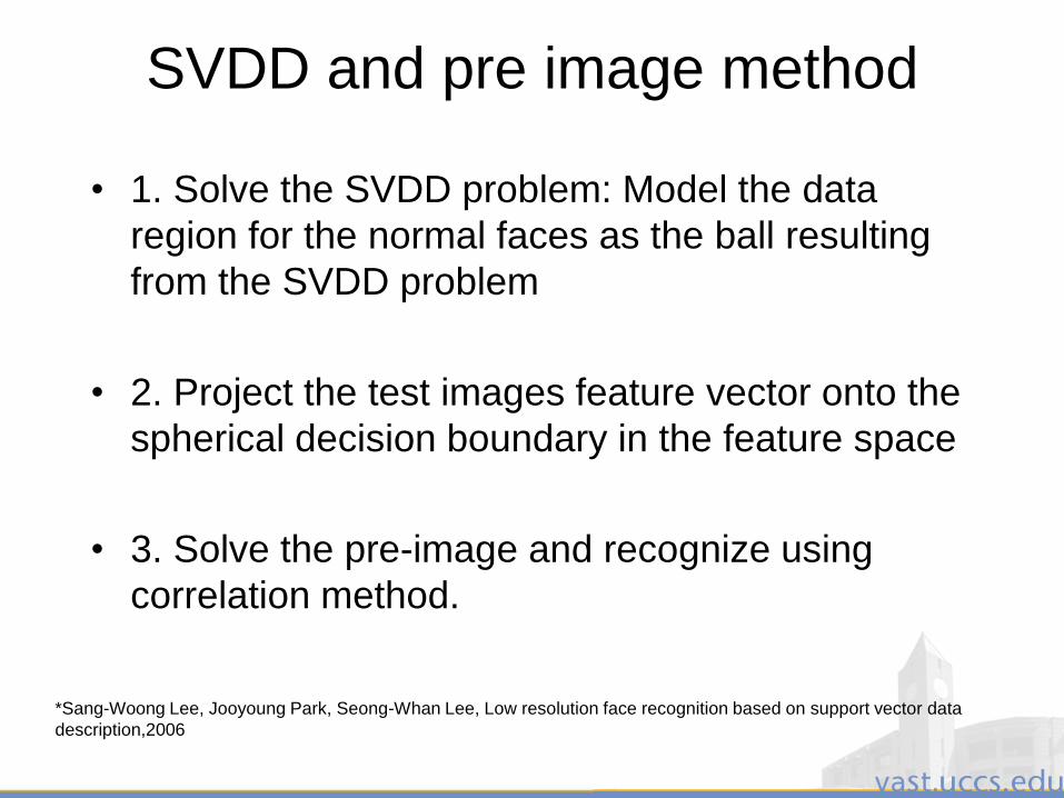
SVDD and pre image method
• 1. Solve the SVDD problem: Model the data
region for the normal faces as the ball resulting
from the SVDD problem
• 2. Project the test images feature vector onto the
spherical decision boundary in the feature space
• 3. Solve the pre-image and recognize using
correlation method.
*Sang-Woong Lee, Jooyoung Park, Seong-Whan Lee, Low resolution face recognition based on support vector data
description,2006
3/28/2011 173
Some conclusions from S-R methods
• Fully automated rank 1 recognition rates are still likely
to be poor despite the improvement provided by super-
resolution. A fully automated recognition system is
currently impractical.
• The surveillance system will need to operate in a semi-
automated manner by generating a list of top machine
matches for subsequent analysis by humans.
*Seong-Whan Lee, Stan Li, Frank Lin, Clinton Fookes, Vinod Chandran, Sridha Sridharan “ Super-
Resolved Faces for Improved Face Recognition from Surveillance Video”,2007

3/28/2011 174
Thoughts on Super Resolution
and its Applicability
3/28/2011 175
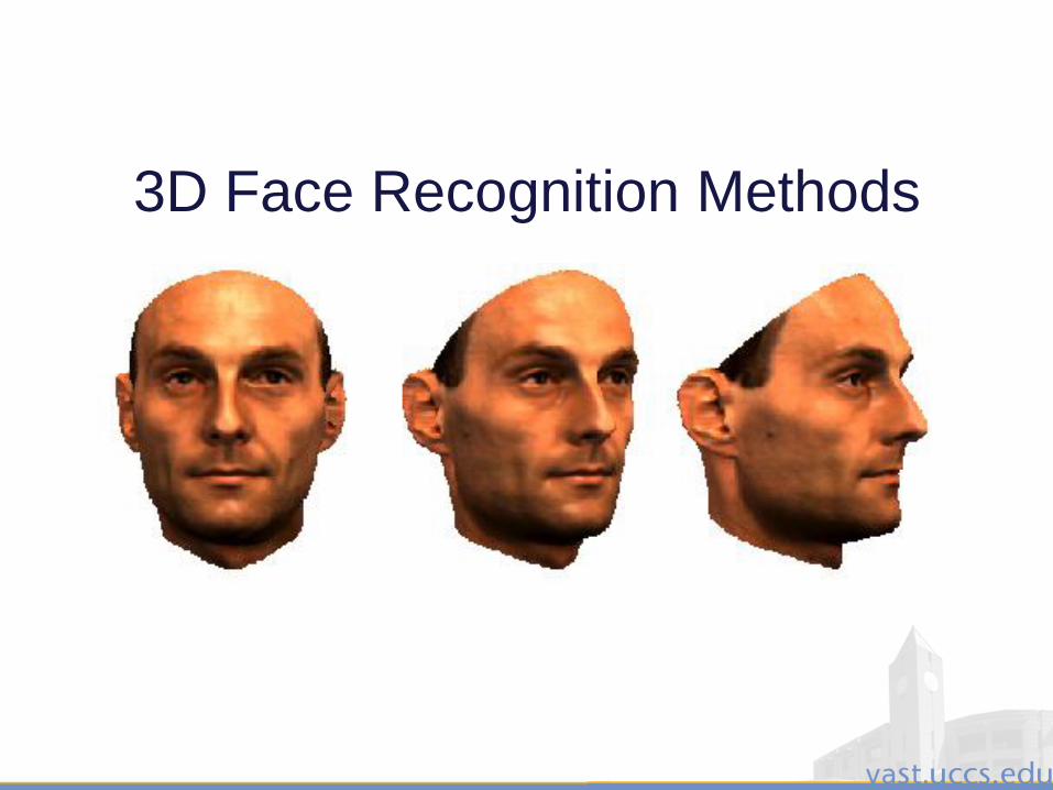
3D Face Recognition Methods
3/28/2011 176
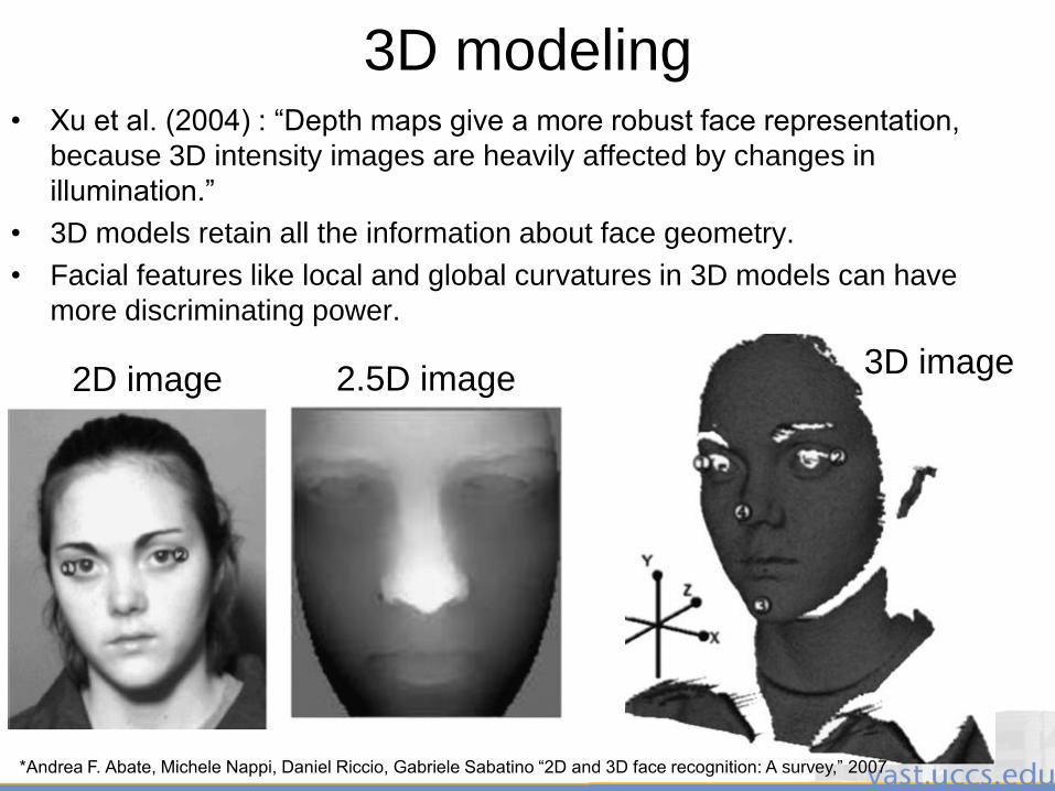
3D modeling • Xu et al. (2004) : “Depth maps give a more robust face representation,
because 3D intensity images are heavily affected by changes in
illumination.”
• 3D models retain all the information about face geometry.
• Facial features like local and global curvatures in 3D models can have
more discriminating power.
2D image 2.5D image3D image
*Andrea F. Abate, Michele Nappi, Daniel Riccio, Gabriele Sabatino “2D and 3D face recognition: A survey,” 2007
3/28/2011 177
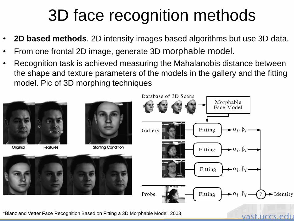
3D face recognition methods
• 2D based methods. 2D intensity images based algorithms but use 3D data.
• From one frontal 2D image, generate 3D morphable model.
• Recognition task is achieved measuring the Mahalanobis distance between
the shape and texture parameters of the models in the gallery and the fitting
model. Pic of 3D morphing techniques
*Blanz and Vetter Face Recognition Based on Fitting a 3D Morphable Model, 2003
3/28/2011 178
3D face Recognition Methods
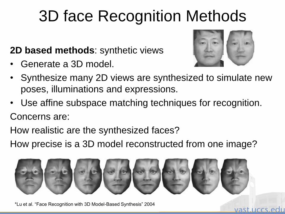
2D based methods: synthetic views
• Generate a 3D model.
• Synthesize many 2D views are synthesized to simulate new
poses, illuminations and expressions.
• Use affine subspace matching techniques for recognition.
Concerns are:
How realistic are the synthesized faces?
How precise is a 3D model reconstructed from one image?
*Lu et al. “Face Recognition with 3D Model-Based Synthesis” 2004
3/28/2011 179
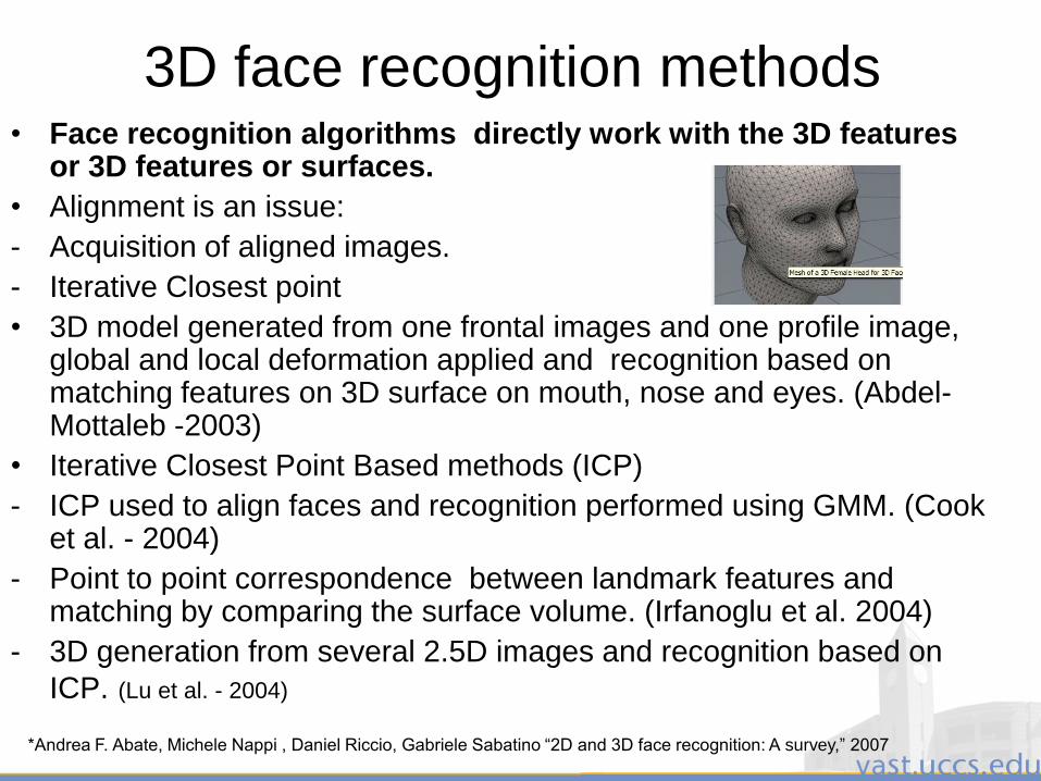
3D face recognition methods• Face recognition algorithms directly work with the 3D features
or 3D features or surfaces.
• Alignment is an issue:
- Acquisition of aligned images.
- Iterative Closest point
• 3D model generated from one frontal images and one profile image, global and local deformation applied and recognition based on matching features on 3D surface on mouth, nose and eyes. (Abdel-Mottaleb -2003)
• Iterative Closest Point Based methods (ICP)
- ICP used to align faces and recognition performed using GMM. (Cook et al. - 2004)
- Point to point correspondence between landmark features and matching by comparing the surface volume. (Irfanoglu et al. 2004)
- 3D generation from several 2.5D images and recognition based on
ICP. (Lu et al. - 2004)
*Andrea F. Abate, Michele Nappi , Daniel Riccio, Gabriele Sabatino “2D and 3D face recognition: A survey,” 2007
3/28/2011 180
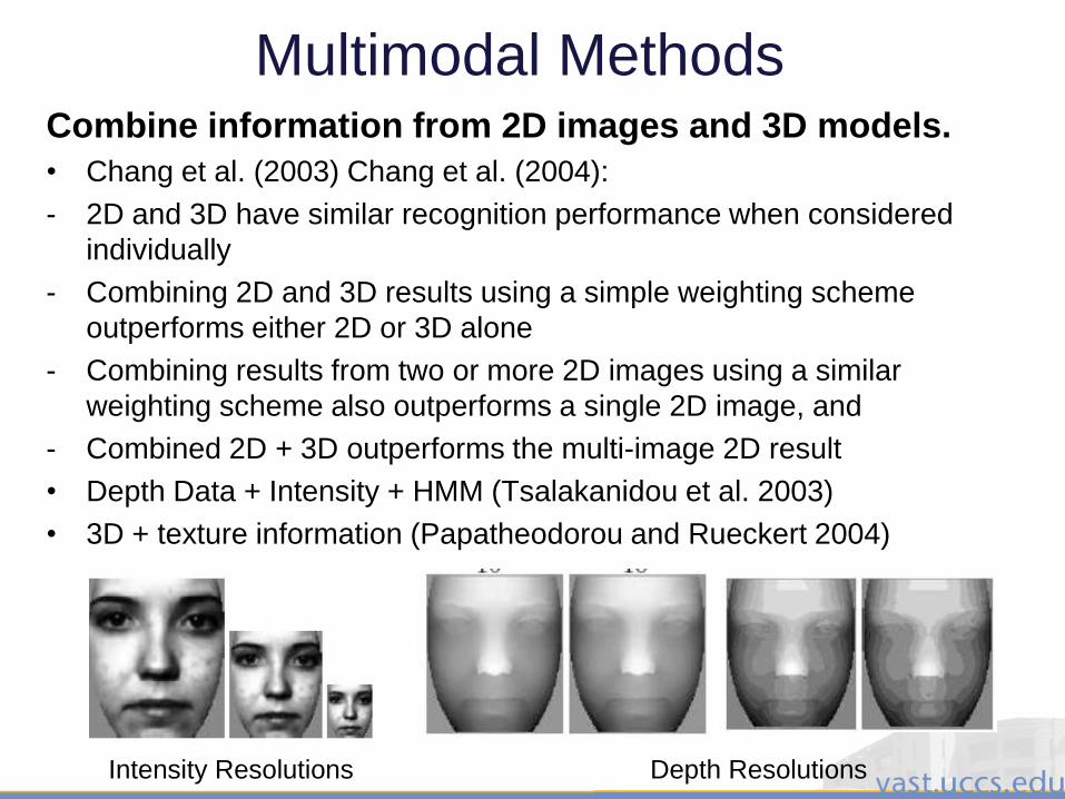
Multimodal MethodsCombine information from 2D images and 3D models.
• Chang et al. (2003) Chang et al. (2004):
- 2D and 3D have similar recognition performance when considered
individually
- Combining 2D and 3D results using a simple weighting scheme
outperforms either 2D or 3D alone
- Combining results from two or more 2D images using a similar
weighting scheme also outperforms a single 2D image, and
- Combined 2D + 3D outperforms the multi-image 2D result
• Depth Data + Intensity + HMM (Tsalakanidou et al. 2003)
• 3D + texture information (Papatheodorou and Rueckert 2004)
Intensity Resolutions Depth Resolutions
3/28/2011 181
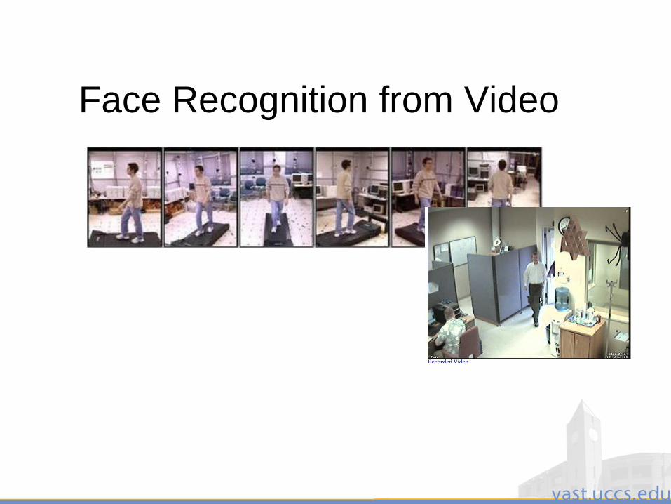
Face Recognition from Video
3/28/2011 182
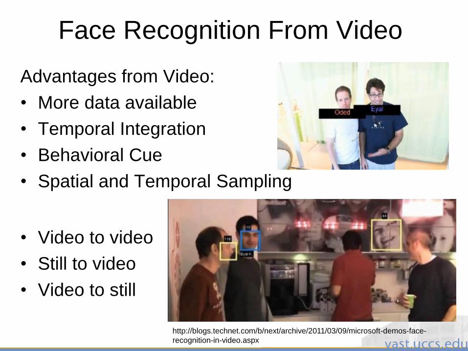
Face Recognition From Video
Advantages from Video:
• More data available
• Temporal Integration
• Behavioral Cue
• Spatial and Temporal Sampling
• Video to video
• Still to video
• Video to still
http://blogs.technet.com/b/next/archive/2011/03/09/microsoft-demos-face-
recognition-in-video.aspx

3/28/2011 183
Face Recognition From Video
The curse of Dimensionality
The risk is to have too much data to be processed
How to exploit the added information in video?
Standard VGA (640x480)
1 frame: 300 KByte
30 frames: 1 MByte
Standard video: ~1 MByte/Sec
3/28/2011 184
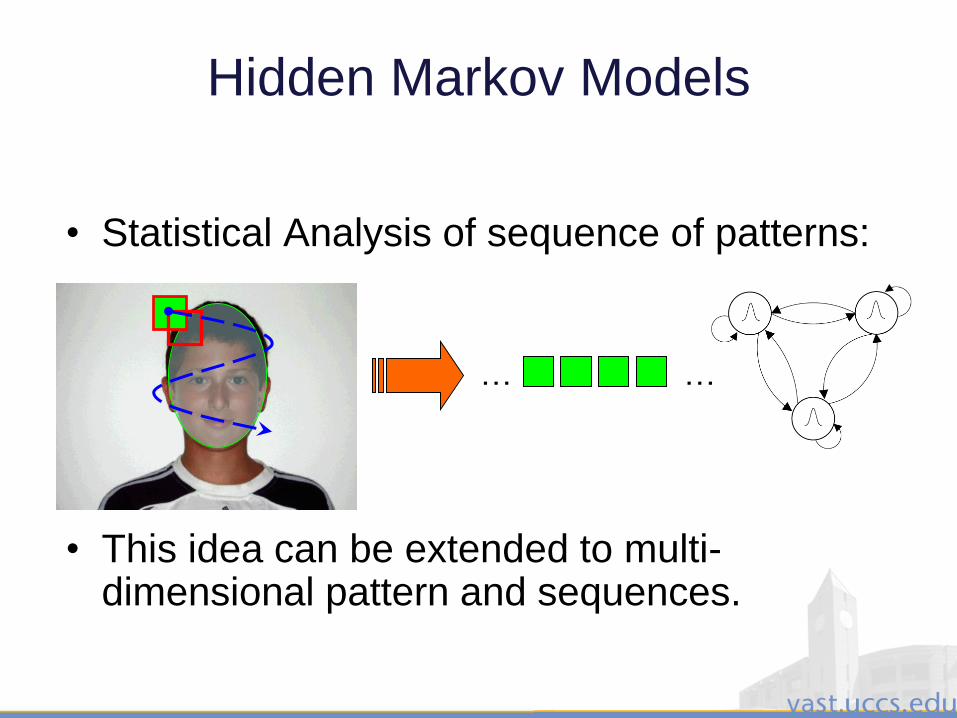
Hidden Markov Models
• Statistical Analysis of sequence of patterns:
• This idea can be extended to multi-dimensional pattern and sequences.
… …

3/28/2011 185
Dynamic Hidden Markov Model
• Each image is modeled as a single HMM and the sequence of images as a sequence of HMMs
(A. Hadid and M. Pietikainen. “An experimental investigation about the integration of facial dynamics in video-based face recognition”. Electronic Letters on Computer Vision and Image Analysis, 5(1):1-13, 2005.)
• The entire video is modeled as a single HMM
(X. Liu and T. Chen. “Video-based face recognition using adaptive hidden Markov models”. In Proc. Int. Conf. on Computer Vision and Pattern Recognition, 2003.)
• The images and the sequence itself are modeled as a complex, hierarchical HMM-based structure
(M. Bicego, E.Grosso, M. Tistarelli. “Person authentication from video of faces: a behavioural and physiological approach using Pseudo Hierarchical Hidden Markov Models”, Intl. Conference on Biometric Authentication 2006, Hong Kong, China, January 2006. )
3/28/2011 186
Face Recognition from Video
Not just more data to be processes, the issues are:
• Data selection (pose, expression, illumination,
noise…)
• Multi-data fusion (decision/score/feature level)
• 3D reconstruction/virtual views
• Resolution enhancement
• Expression and emotion analysis
• Behavioral analysis
• Dynamic video templates…?
3/28/2011 187
Face Recognition in Video
• Probabilistic recognition of human faces from video1
- The joint posterior distribution of the motion vector and the identity variable is estimated using Sequential Importance Sampling at each time instant and then propagated to the next time instant.
• Video based face recognition using probabilistic appearance manifolds2
- Each registered person is represented by a low-dimensional appearance manifold in the ambient image space.
- A maximum a posteriori formulation performed on test images by integrating the likelihood that the input image comes from a particular pose manifold and the transition probability to this pose manifold from the previous frame.
1. R. Chellappa, V. Kruger, S. Zhou, “Probabilistic recognition of human faces from video,” 2002.
2. K. Lee, J. Ho, M. Yang and D. Kriegman, “Video based face recognition using probabilistic
appearance manifolds,” 2003
3/28/2011 188
Findings from Video based Analysis*
• Important findings:
• Short sequences do not have enough dynamic information to discriminate between individuals. So spatio-temporal algorithms may not do well when there is a short sequence.
• However, with a longer sequence good facial dynamics are achieved and spatio-temporal methods do well.
• Open question: How representative the face sequences should be in order to allow the system to learn the dynamics of each individual.
• Image quality affects both the representations, but image based methods are more affected. So for the face recognition with low quality images, spatio-temporal representations are more suitable.
• More than just rigid head motion, expressions or talking or laughing can add dynamics to face recognition.
*A. Hadid, M. Pietikinen, "From Still Image to Video-Based Face Recognition: An Experimental Analysis,” 2004
3/28/2011 189
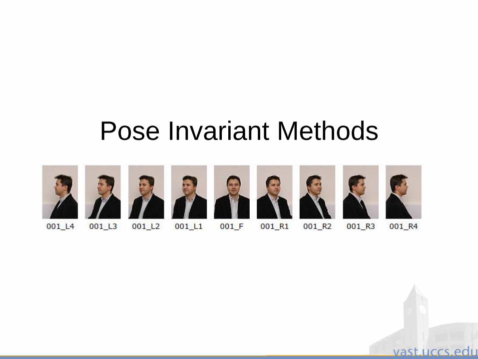
Pose Invariant Methods
3/28/2011 190
Pose Invariant Features
• Local approaches such as EBGM and LBP are more robust to pose variations than holistic approaches such as PCA and LDA. This is because local approaches are relatively less dependent on pixel-wise correspondence between gallery and probe images, which is adversely affected by pose variations
• The tolerance of local approaches to pose variations is limited to small in-depth rotations.
• These methods are not entirely robust to pose variations, because distortions exist in local image regions under pose variations.
• Under intermediate or large pose variations, pose compensation or specific pose-invariant feature extraction is necessary and beneficial.

3/28/2011 191
Pose Invariant Features
• Four-point cross ratio and others.
*Joseph L. Mundy, Andrew Zisserman, Geometric invariance in computer vision
• Affine transformation invariant features*Wide Baseline stereo matching based on locally affine invariant regions;
An affine invariant interest point detector
• General transformation invariant features*Automatic acquisition of exemplar based representations for recognition from image sequences.
• Problems: Many features which are important for recognition are not selected as pose invariant and many selected features are not sufficient for recognition especially in a situation like face recognition.
• Affine invariant patches do not work for 45 degree or more rotation.

3/28/2011 192
Pose Invariant Methods• Real View Based Matching: Multiple gallery
view of every subject to be matched.• D.J. Beymer, 1994
• R. Singh et al.(2007)
• Challenge: it is generally impractical to collect multiple images in different poses for real view-based matching
• 3D models based methods
• 3D shape Models, feature based 3D reconstruction, image based 3D reconstruction
3/28/2011 193
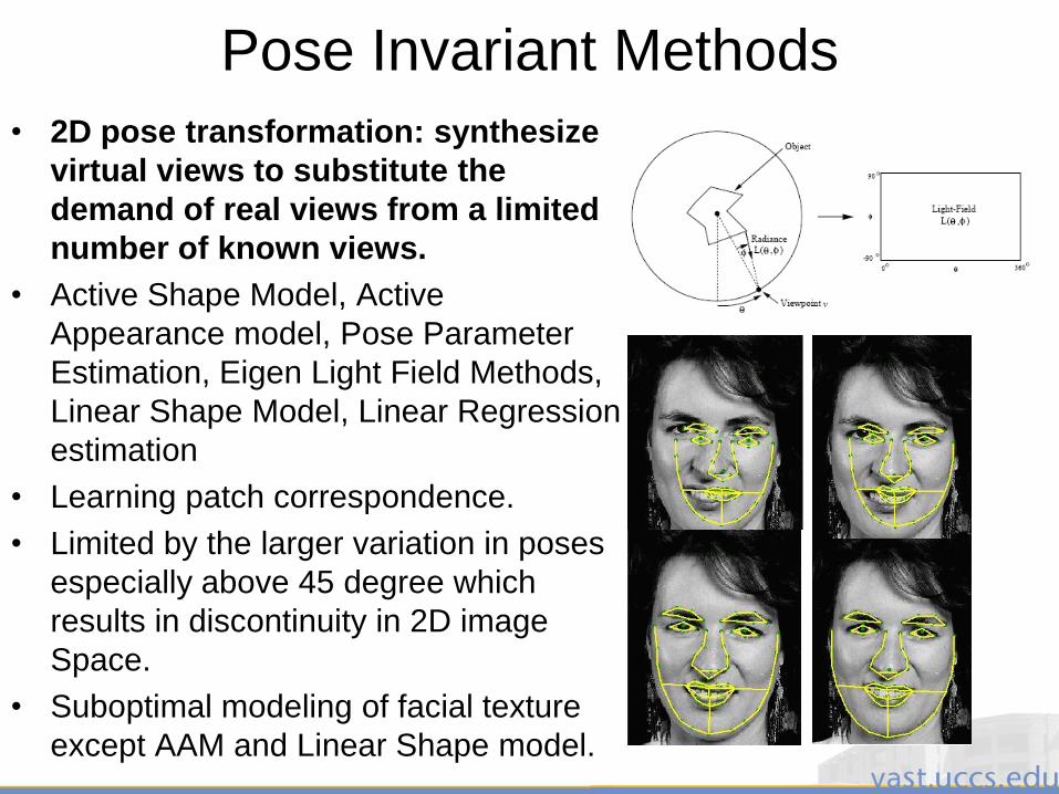
Pose Invariant Methods
• 2D pose transformation: synthesize
virtual views to substitute the
demand of real views from a limited
number of known views.
• Active Shape Model, Active
Appearance model, Pose Parameter
Estimation, Eigen Light Field Methods,
Linear Shape Model, Linear Regression
estimation
• Learning patch correspondence.
• Limited by the larger variation in poses
especially above 45 degree which
results in discontinuity in 2D image
Space.
• Suboptimal modeling of facial texture
except AAM and Linear Shape model.
3/28/2011 194
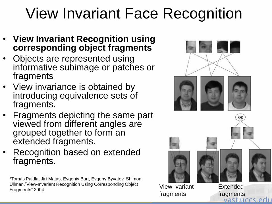
View Invariant Face Recognition
• View Invariant Recognition using corresponding object fragments
• Objects are represented using informative subimage or patches or fragments
• View invariance is obtained by introducing equivalence sets of fragments.
• Fragments depicting the same part viewed from different angles are grouped together to form an extended fragments.
• Recognition based on extended fragments.
View variant
fragments
Extended
fragments
*Tomás Pajdla, Jirí Matas, Evgeniy Bart, Evgeny Byvatov, Shimon
Ullman,”View-Invariant Recognition Using Corresponding Object
Fragments” 2004
3/28/2011 195
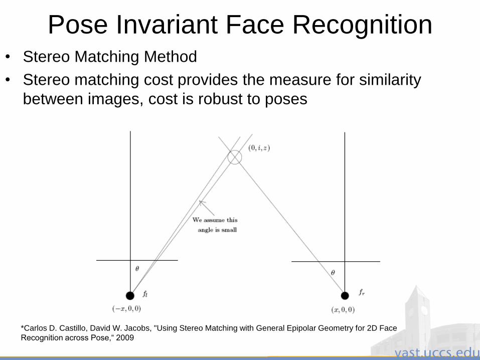
Pose Invariant Face Recognition• Stereo Matching Method
• Stereo matching cost provides the measure for similarity
between images, cost is robust to poses
*Carlos D. Castillo, David W. Jacobs, "Using Stereo Matching with General Epipolar Geometry for 2D Face
Recognition across Pose,“ 2009
3/28/2011 196
Occlusion Invariant Methods

3/28/2011 197
Occlusion Invariant Methods• Robust Face recognition via sparse Representation.
• If sparsity in the recognition problem is properly harnessed, the
choice of features is no longer critical however the choice of the
number of features is still critical.
• Test image can be represented as a linear combination of training
samples and the identity can be found out by solving the linear
representation (solving l1 norm minimization problem).
*John Wright, Allen Y. Yang, Arvind Ganesh, S. Shankar Sastry, Yi Ma, "Robust Face Recognition via
Sparse Representation,” 2007
3/28/2011 198
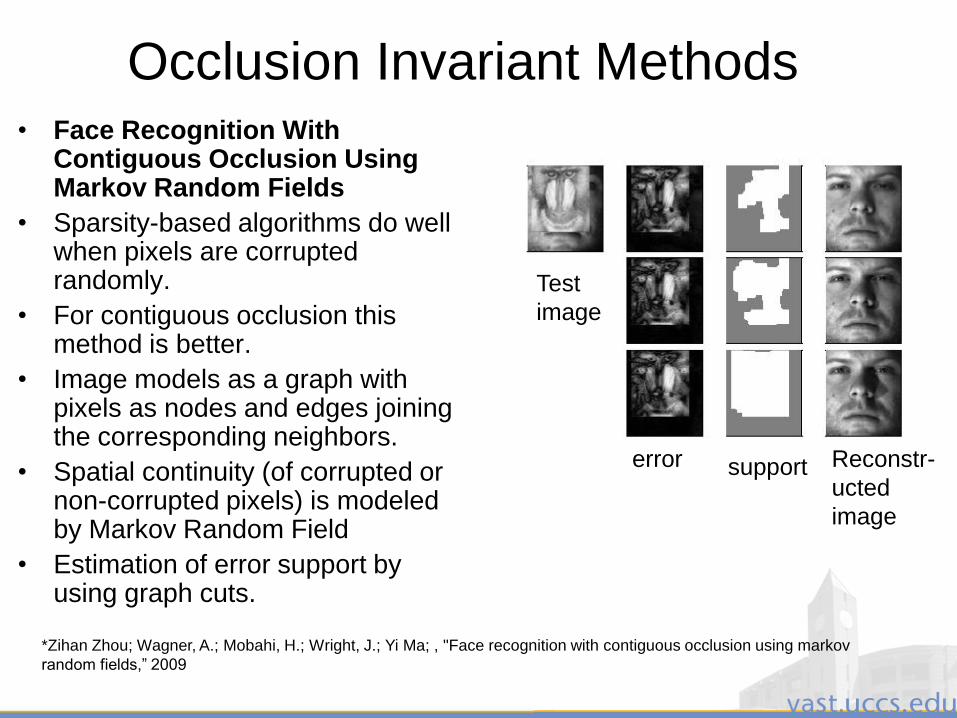
Occlusion Invariant Methods• Face Recognition With
Contiguous Occlusion Using Markov Random Fields
• Sparsity-based algorithms do well when pixels are corrupted randomly.
• For contiguous occlusion this method is better.
• Image models as a graph with pixels as nodes and edges joining the corresponding neighbors.
• Spatial continuity (of corrupted or non-corrupted pixels) is modeled by Markov Random Field
• Estimation of error support by using graph cuts.
Test
image
error support Reconstr-
ucted
image
*Zihan Zhou; Wagner, A.; Mobahi, H.; Wright, J.; Yi Ma; , "Face recognition with contiguous occlusion using markov
random fields,” 2009
3/28/2011 199
Thermal Imaging
3/28/2011 200
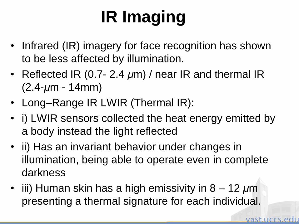
IR Imaging
• Infrared (IR) imagery for face recognition has shown
to be less affected by illumination.
• Reflected IR (0.7- 2.4 μm) / near IR and thermal IR
(2.4-μm - 14mm)
• Long–Range IR LWIR (Thermal IR):
• i) LWIR sensors collected the heat energy emitted by
a body instead the light reflected
• ii) Has an invariant behavior under changes in
illumination, being able to operate even in complete
darkness
• iii) Human skin has a high emissivity in 8 – 12 μm
presenting a thermal signature for each individual.

3/28/2011 201
Thermal Imaging
• Challenges
• Thermal signatures can be changed significantly according to different body temperatures caused by physical exercise or ambient temperatures.
• Thermal images of a subject wearing eyeglasses may lose information around the eyes since glass blocks a large portion of thermal energy.
• Thermal imaging has difficulty in recognizing people inside a moving vehicle.
3/28/2011 202
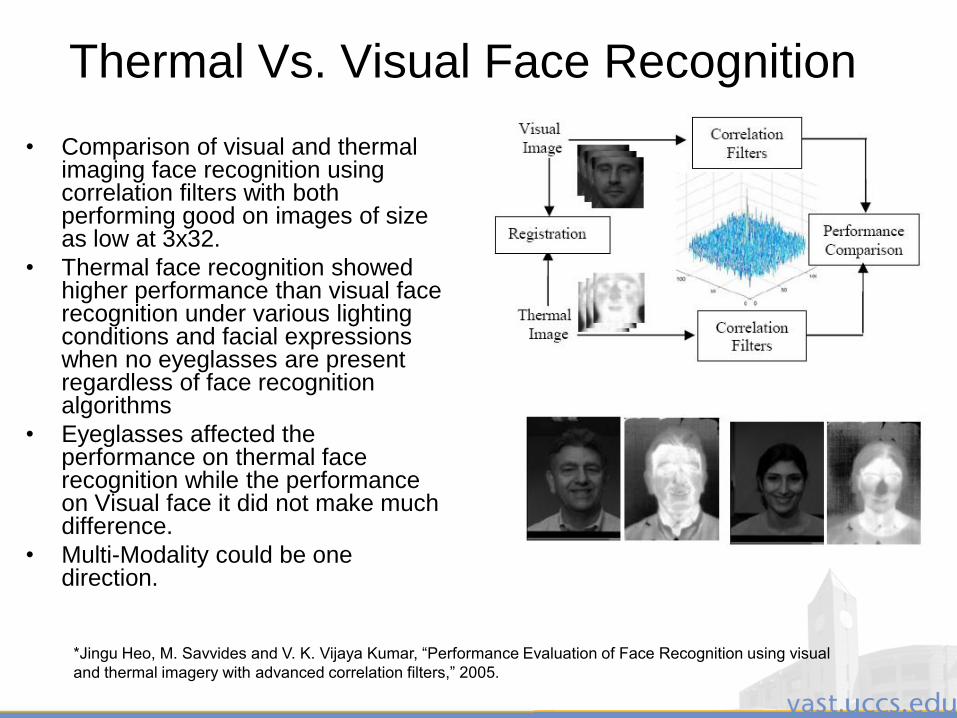
Thermal Vs. Visual Face Recognition
• Comparison of visual and thermal imaging face recognition using correlation filters with both performing good on images of size as low at 3x32.
• Thermal face recognition showed higher performance than visual face recognition under various lighting conditions and facial expressions when no eyeglasses are present regardless of face recognition algorithms
• Eyeglasses affected the performance on thermal face recognition while the performance on Visual face it did not make much difference.
• Multi-Modality could be one direction.
*Jingu Heo, M. Savvides and V. K. Vijaya Kumar, “Performance Evaluation of Face Recognition using visual
and thermal imagery with advanced correlation filters,” 2005.
3/28/2011 203
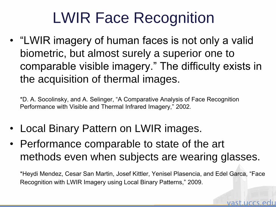
LWIR Face Recognition
• “LWIR imagery of human faces is not only a valid
biometric, but almost surely a superior one to
comparable visible imagery.” The difficulty exists in
the acquisition of thermal images.
*D. A. Socolinsky, and A. Selinger, “A Comparative Analysis of Face Recognition
Performance with Visible and Thermal Infrared Imagery,” 2002.
• Local Binary Pattern on LWIR images.
• Performance comparable to state of the art
methods even when subjects are wearing glasses.
*Heydi Mendez, Cesar San Martin, Josef Kittler, Yenisel Plasencia, and Edel Garca, “Face
Recognition with LWIR Imagery using Local Binary Patterns,” 2009.
3/28/2011 204
LWIR Face Recognition
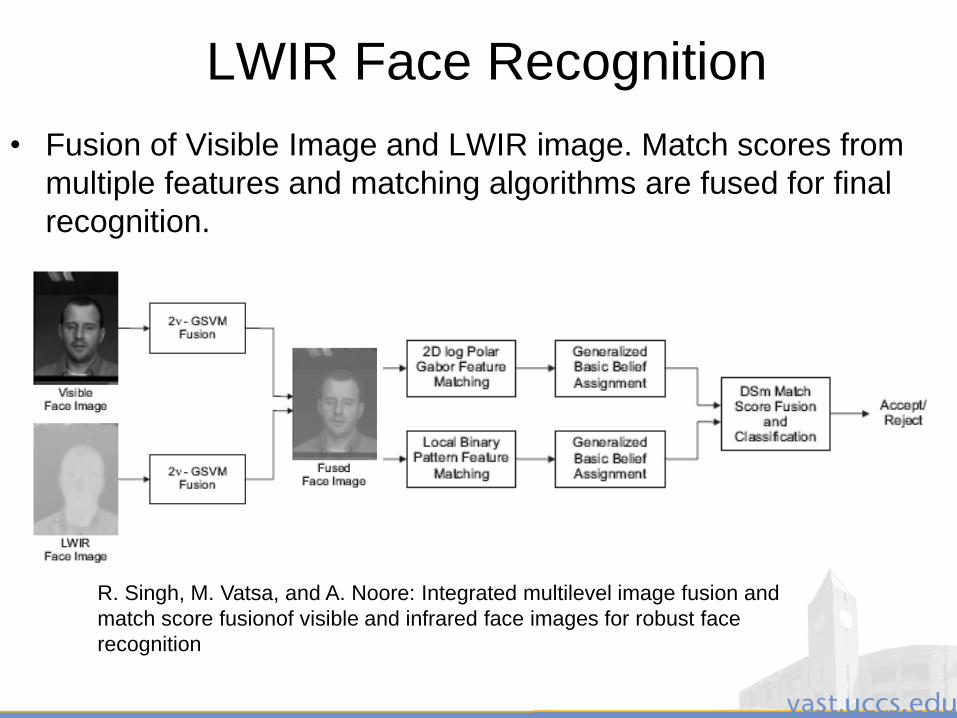
• Fusion of Visible Image and LWIR image. Match scores from
multiple features and matching algorithms are fused for final
recognition.
R. Singh, M. Vatsa, and A. Noore: Integrated multilevel image fusion and
match score fusionof visible and infrared face images for robust face
recognition
3/28/2011 205
Biologically Inspired Methods
3/28/2011 206
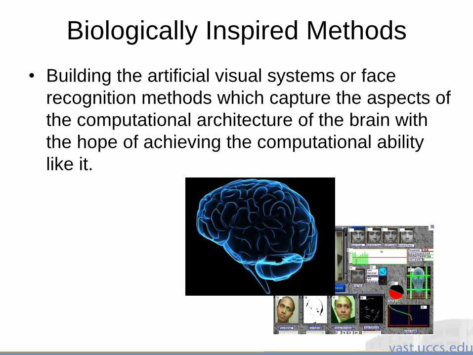
Biologically Inspired Methods
• Building the artificial visual systems or face
recognition methods which capture the aspects of
the computational architecture of the brain with
the hope of achieving the computational ability
like it.
3/28/2011 207
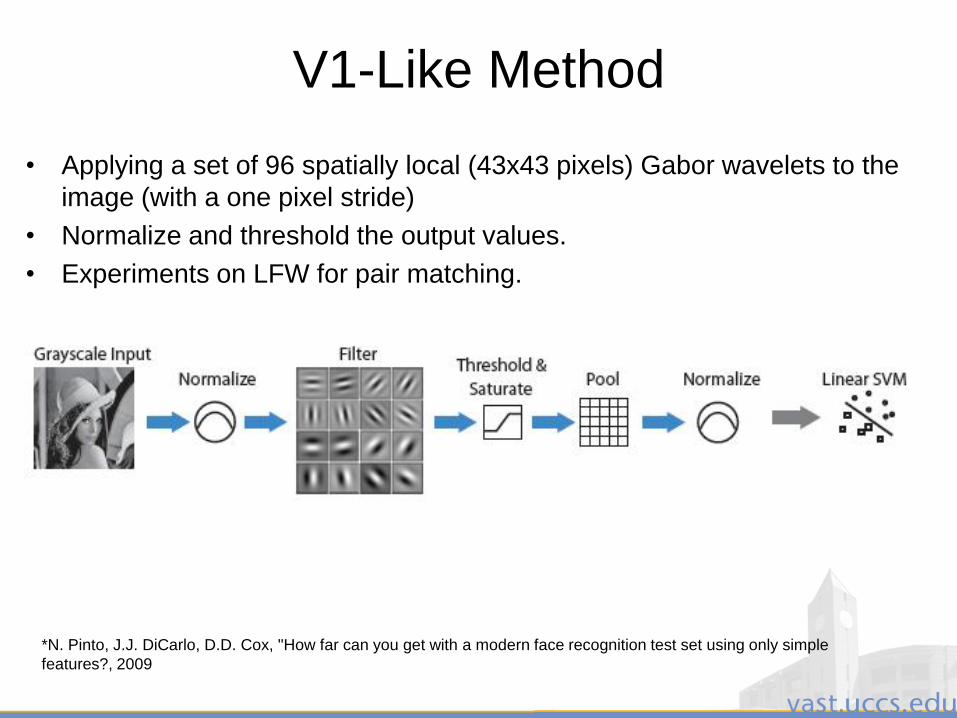
V1-Like Method
• Applying a set of 96 spatially local (43x43 pixels) Gabor wavelets to the
image (with a one pixel stride)
• Normalize and threshold the output values.
• Experiments on LFW for pair matching.
*N. Pinto, J.J. DiCarlo, D.D. Cox, "How far can you get with a modern face recognition test set using only simple
features?, 2009

3/28/2011 208
High Throughput (HT) models
• Composed of a hierarchy of two or three layers.
• Each layer consists of cascade of liner and non-linear
operations which produces the no-linear feature map of
original image.
*N. Pinto, J.J. DiCarlo, D.D. Cox , Beyond Simple Features: A Large-Scale Feature Search Approach to Unconstrained
Face Recognition, F&G 2011
3/28/2011 209
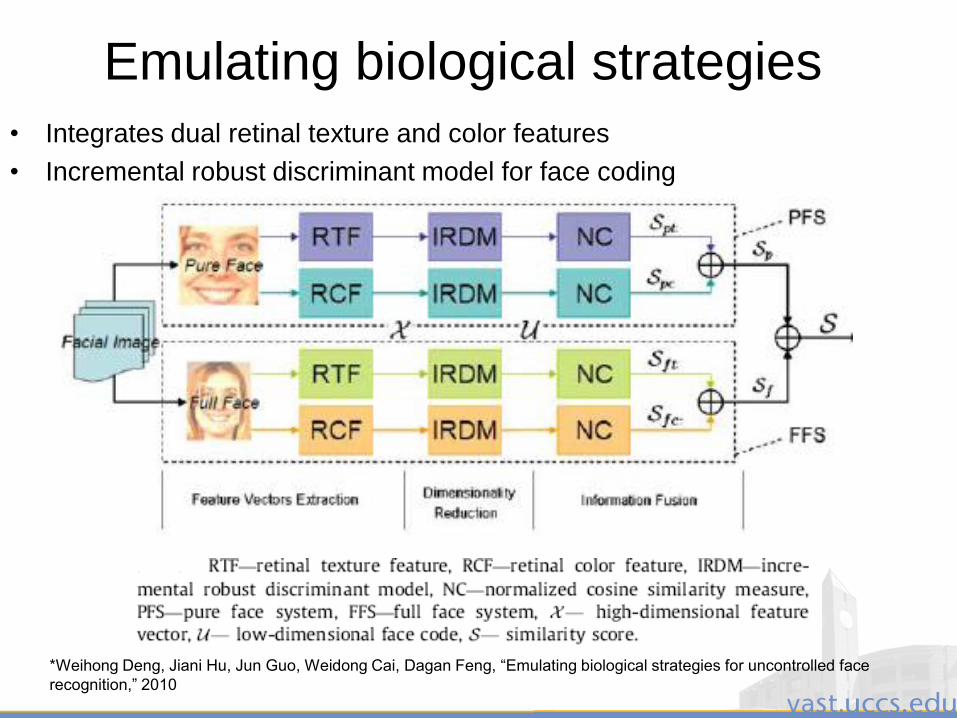
Emulating biological strategies
• Integrates dual retinal texture and color features
• Incremental robust discriminant model for face coding
*Weihong Deng, Jiani Hu, Jun Guo, Weidong Cai, Dagan Feng, “Emulating biological strategies for uncontrolled face
recognition,” 2010
3/28/2011 210
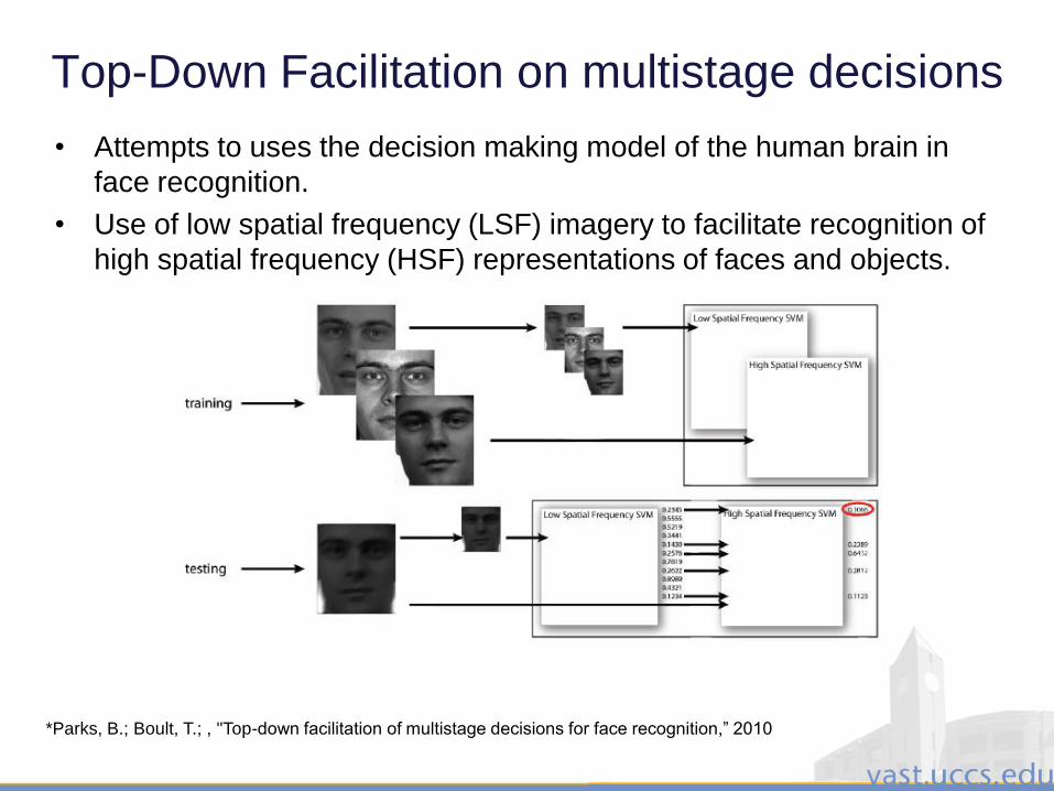
Top-Down Facilitation on multistage decisions
• Attempts to uses the decision making model of the human brain in
face recognition.
• Use of low spatial frequency (LSF) imagery to facilitate recognition of
high spatial frequency (HSF) representations of faces and objects.
*Parks, B.; Boult, T.; , "Top-down facilitation of multistage decisions for face recognition,” 2010
3/28/2011 211
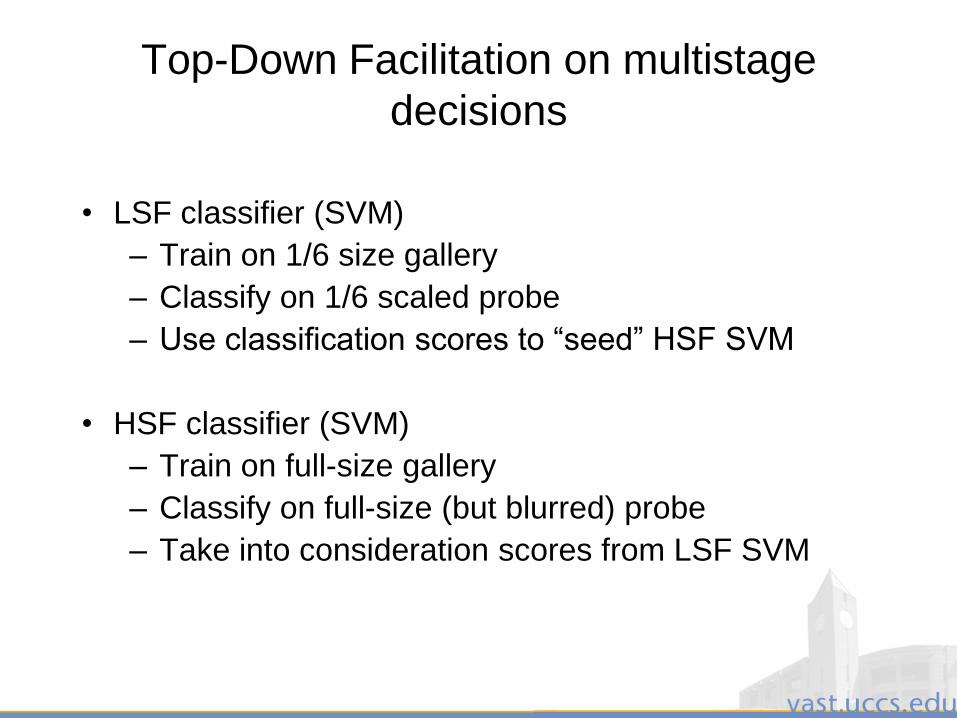
Top-Down Facilitation on multistage
decisions
• LSF classifier (SVM)
– Train on 1/6 size gallery
– Classify on 1/6 scaled probe
– Use classification scores to “seed” HSF SVM
• HSF classifier (SVM)
– Train on full-size gallery
– Classify on full-size (but blurred) probe
– Take into consideration scores from LSF SVM
3/28/2011 212
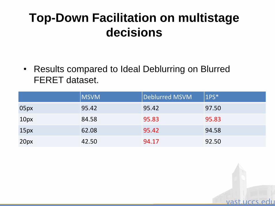
Top-Down Facilitation on multistage
decisions
• Results compared to Ideal Deblurring on Blurred
FERET dataset.
MSVM Deblurred MSVM 1PS*
05px 95.42 95.42 97.50
10px 84.58 95.83 95.83
15px 62.08 95.42 94.58
20px 42.50 94.17 92.50

3/28/2011 213
How can we leverage recent
findings in other sciences?

3/28/2011 214
Future Directions for Uncontrolled Face
Recognition
• One system to solve all the problems?
• Multi-modality, features, methods, recognition score
fusion
• More work on configurable information
• Consider „familiarity‟
• Top Down expectations
• Long distance recognition: acquisition, preprocessing
and recognition
• Face Recognition in camera network
*Rama Chellappa, Pawan Sinha, P. Jonathon Phillips, “Face Recognition by Computers and
Humans”, 2010.
3/28/2011 215
Popular Classification Methods
• Distance measures:
- Similarity or differences between the features
using various distance functions. City block,
cosine, etc.
- Statistical distances for the feature distributions:
Bhattacharyya distance, Earth mover's distance,
Mahalanobis distance etc.
- Normalized cross correlation.
- Bayesian Classifier

3/28/2011 216
Support vector machines.
The separating hyperplane can be very complex
Problems may occur with outliers
The shape of the hyperplane depends on the population of the
Classes
Need for negative examples
3/28/2011 217
Hidden Markov Models
Coding– the image is scanned to obtain a sequence of T partially
overlapped sub-images
– for each sub-image the DCT coefficients are computed
– only the most important D coefficients are retained
– the final sequence is composed by DxT symbols
Learning: train one HMM for each subject:– the number of states is fixed a priori
– at the end we have one HMM for each subject
Recognition: – Bayesian scheme: assuming a priori equally probable
classes, an object is assigned to the class whose model shows the highest likelihood (Maximum Likelihood scheme)

3/28/2011 218
Quality and Post Recognition
Score Analysis

3/28/2011 219
Findings from FRVT 2006
• Covariates: factors independent of an
algorithm that may affect performance
– Gender
– Race
– Size of the Face
– Degree of Focus of Face
– Wearing Glasses
– Indoor our Outdoor Imagery
– False Accept Rate
*J. Ross Beveridge, G. Givens, P.J. Philips, B. Draper and Y. Lui, “Focus on
Quality, Predicting FRVT Performance,” 2008.

3/28/2011 220
Face Region in Focus Measure (FRIFM)
• Face is transformed to a standard size
• Sobel edge mask is applied to the image to derive
edges
• Average the Sobel edge magnitude within an oval
defining the region of the face
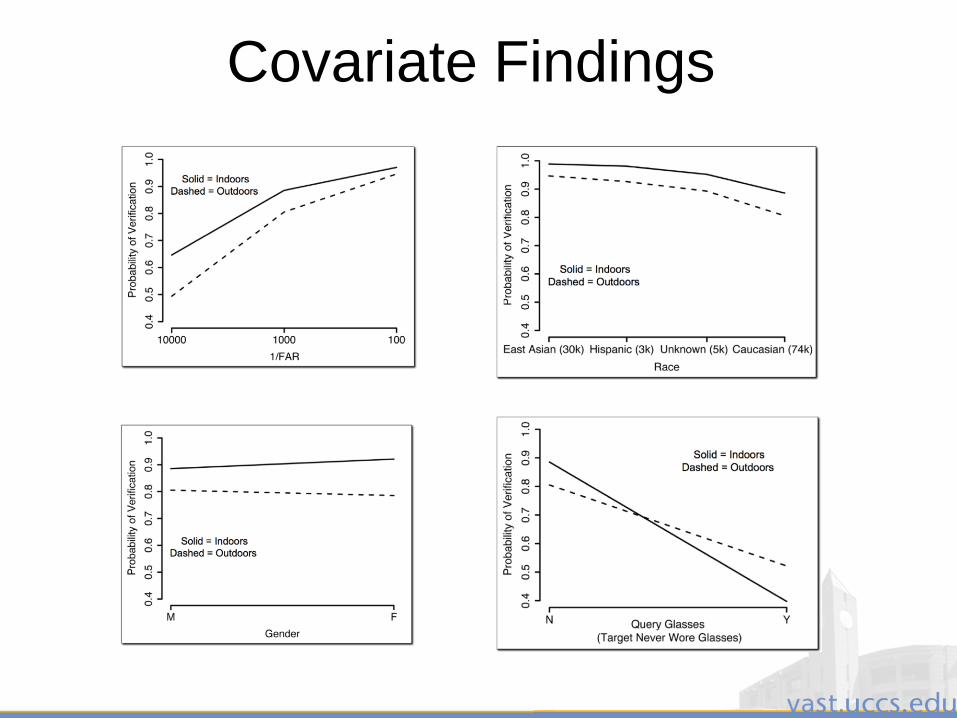
3/28/2011 221
Covariate Findings
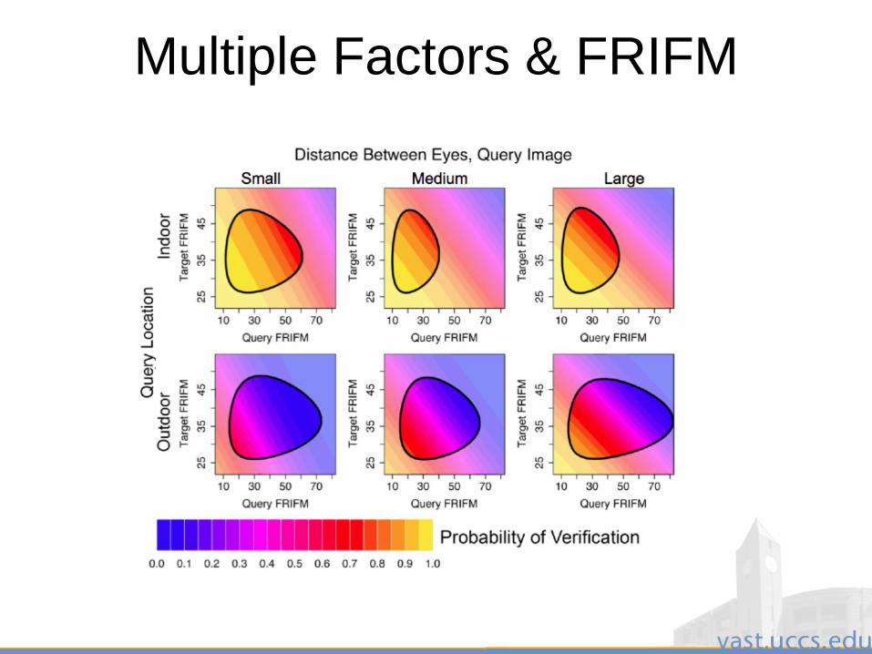
3/28/2011 222
Multiple Factors & FRIFM
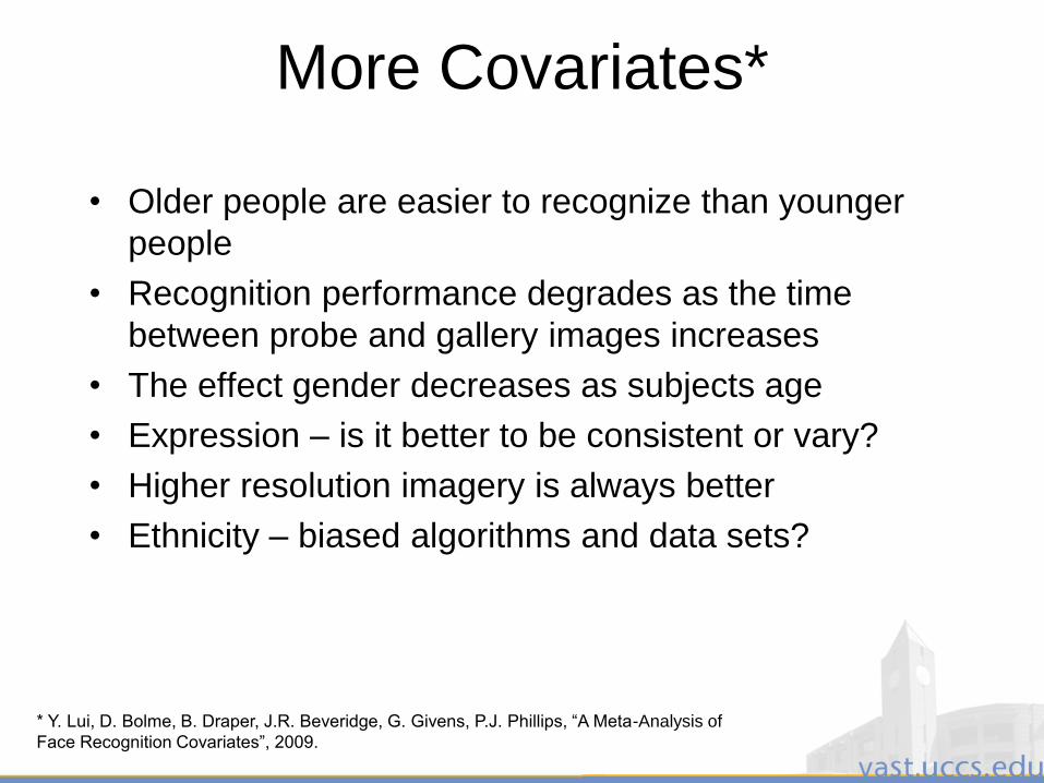
3/28/2011 223
More Covariates*
• Older people are easier to recognize than younger
people
• Recognition performance degrades as the time
between probe and gallery images increases
• The effect gender decreases as subjects age
• Expression – is it better to be consistent or vary?
• Higher resolution imagery is always better
• Ethnicity – biased algorithms and data sets?
* Y. Lui, D. Bolme, B. Draper, J.R. Beveridge, G. Givens, P.J. Phillips, “A Meta-Analysis of
Face Recognition Covariates”, 2009.
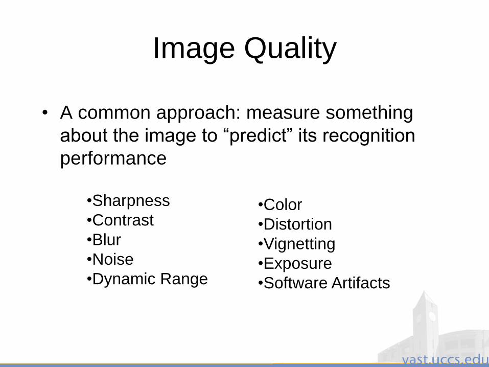
3/28/2011 224
Image Quality
• A common approach: measure something
about the image to “predict” its recognition
performance
•Color
•Distortion
•Vignetting
•Exposure
•Software Artifacts
•Sharpness
•Contrast
•Blur
•Noise
•Dynamic Range
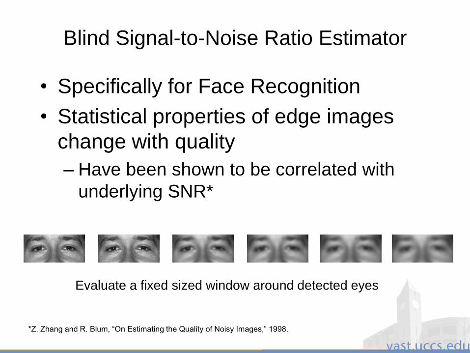
3/28/2011 225
Blind Signal-to-Noise Ratio Estimator
• Specifically for Face Recognition
• Statistical properties of edge images
change with quality
– Have been shown to be correlated with
underlying SNR*
Evaluate a fixed sized window around detected eyes
*Z. Zhang and R. Blum, “On Estimating the Quality of Noisy Images,” 1998.
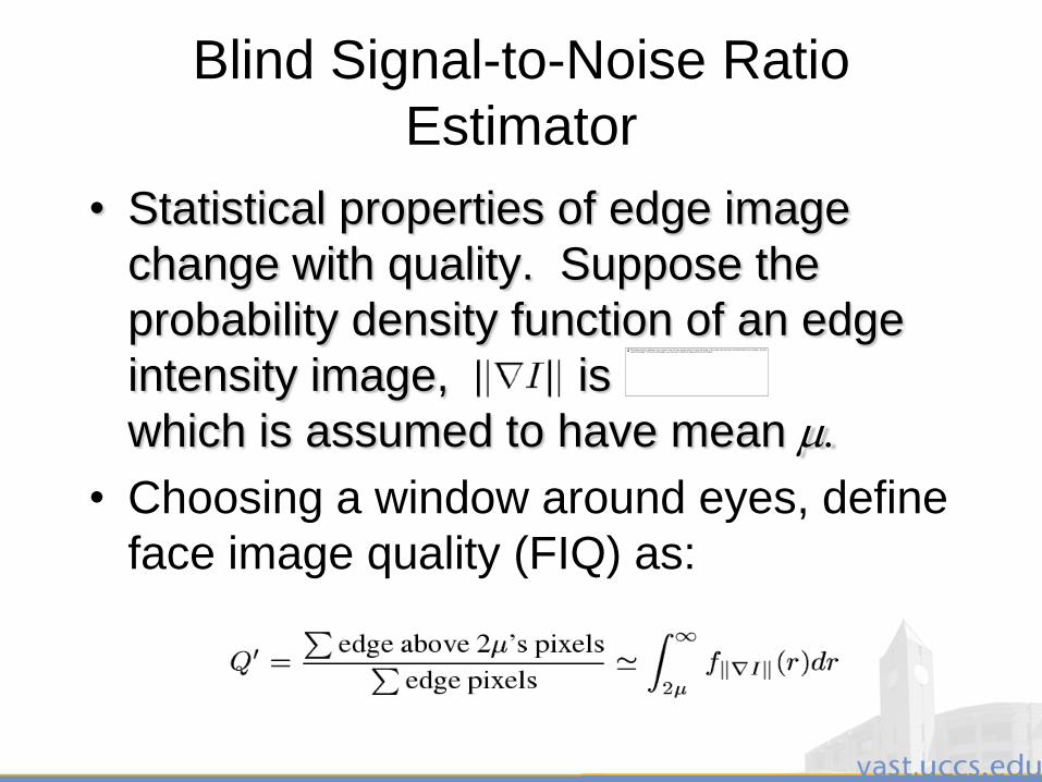
3/28/2011 226
Blind Signal-to-Noise Ratio
Estimator
• Statistical properties of edge image
change with quality. Suppose the
probability density function of an edge
intensity image, is
which is assumed to have mean
• Choosing a window around eyes, define
face image quality (FIQ) as:
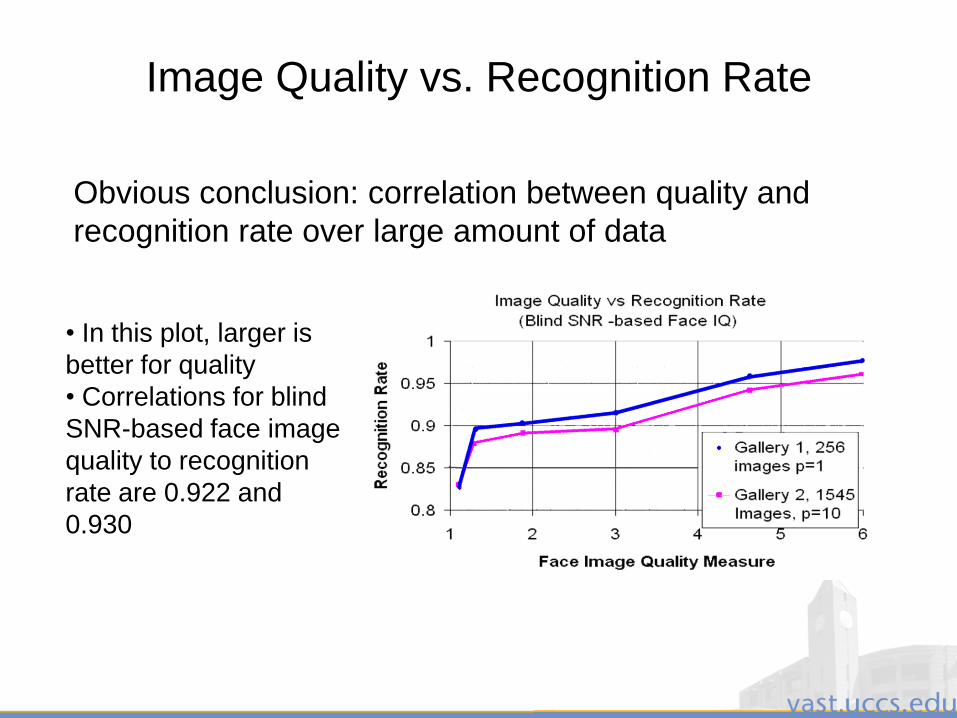
3/28/2011 227
Image Quality vs. Recognition Rate
• In this plot, larger is
better for quality
• Correlations for blind
SNR-based face image
quality to recognition
rate are 0.922 and
0.930
Obvious conclusion: correlation between quality and
recognition rate over large amount of data

3/28/2011 228
Challenges for Image Quality Assessment
• Interesting recent studies from NIST
– Iris1: three different quality assessment
algorithms lacked correlation
– Face2: out of focus imagery was shown to
produce better match scores
1. P. Flynn, “ICE Mining: Quality and Demographic Investigations of ICE 2006 Performance
Results,” MBGC Kick-off workshop, 2008
2. R. Beveridge, “Face Recognition Vendor Test 2006 Experiment 4 Covariate Study,”
MBGC Kick-off workshop, 2008
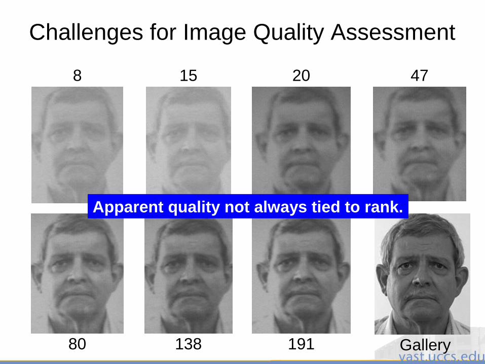
3/28/2011 229
Challenges for Image Quality Assessment
8 15 4720
80 138 191 Gallery
Apparent quality not always tied to rank.
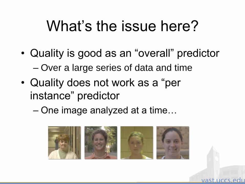
3/28/2011 230
What‟s the issue here?
• Quality is good as an “overall” predictor
– Over a large series of data and time
• Quality does not work as a “per
instance” predictor
– One image analyzed at a time…

3/28/2011 231
“Quality is not in the eye of the beholder;
it is in the recognition performance
figures!” - Ross Beveridge
3/28/2011 232
Biometric Completeness*
• Theory of equivalence in matching and
quality
– A perfect quality measure for any algorithm
would be equivalent to finding a perfect
matching algorithm
– Bounds are placed on the performance of
quality as a predictor
P.J Philips and J.R. Beveridge, “An Introduction to Biometric-Completeness: The Equivalence
of Matching and Quality,” IEEE BTAS, 2009.
3/28/2011 233
Challenges for Image Quality
Assessment
• Alternative to Image Quality Assessment: Post-Recognition Score Analysis
• Predict the performance of a recognition system based on its outputs for each match instance, rather than making decisions about the input imagery
• Meta-Recognition: Control the recognition system by knowing additional information about it
Only the recognition performance figures matter
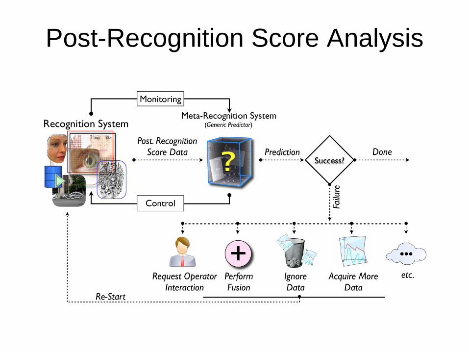
Post-Recognition Score Analysis
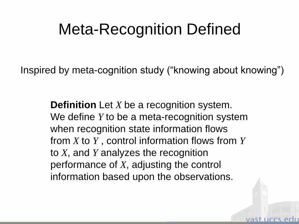
3/28/2011 235
Meta-Recognition Defined
Inspired by meta-cognition study (“knowing about knowing”)
Definition Let X be a recognition system.
We define Y to be a meta-recognition system
when recognition state information flows
from X to Y , control information flows from Y
to X, and Y analyzes the recognition
performance of X, adjusting the control
information based upon the observations.
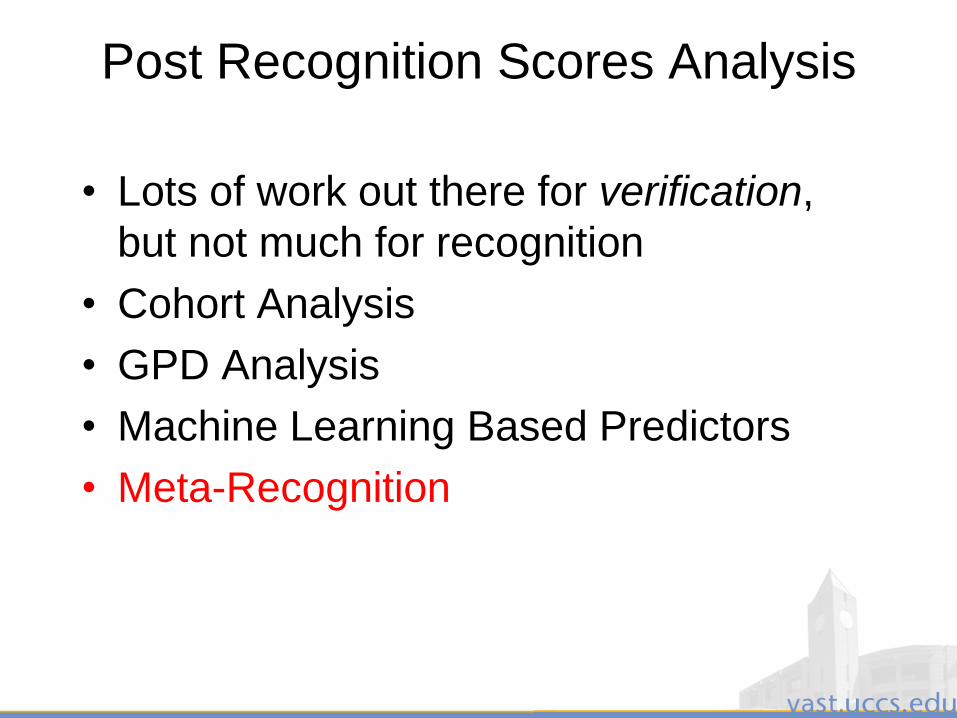
3/28/2011 236
Post Recognition Scores Analysis
• Lots of work out there for verification,
but not much for recognition
• Cohort Analysis
• GPD Analysis
• Machine Learning Based Predictors
• Meta-Recognition
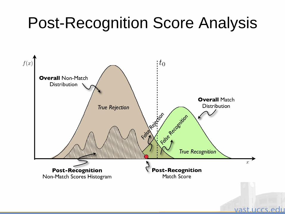
3/28/2011 237
Post-Recognition Score Analysis
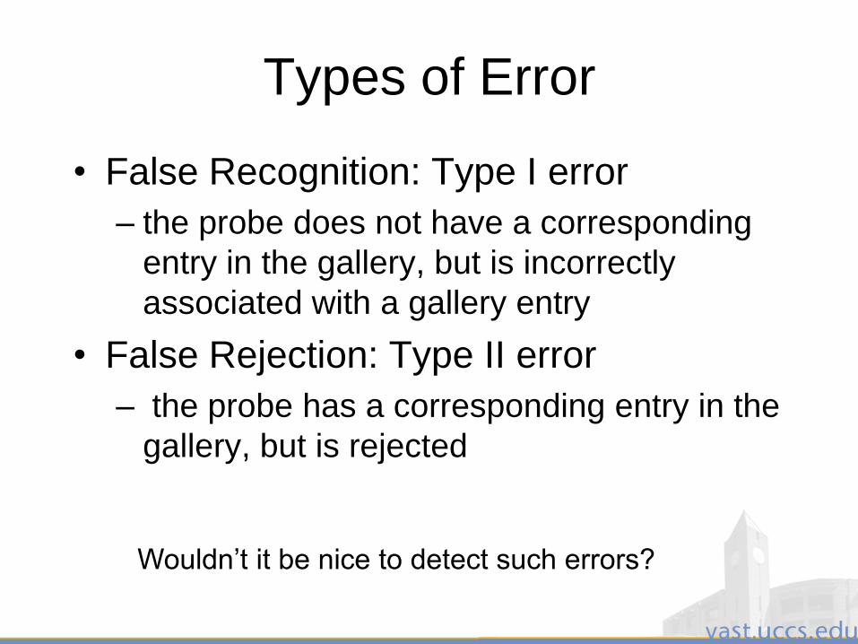
3/28/2011 238
Types of Error
• False Recognition: Type I error
– the probe does not have a corresponding
entry in the gallery, but is incorrectly
associated with a gallery entry
• False Rejection: Type II error
– the probe has a corresponding entry in the
gallery, but is rejected
Wouldn‟t it be nice to detect such errors?
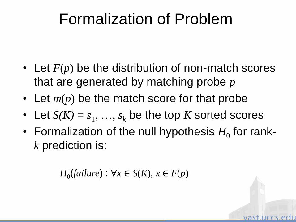
3/28/2011 239
Formalization of Problem
• Let F(p) be the distribution of non-match scores
that are generated by matching probe p
• Let m(p) be the match score for that probe
• Let S(K) = s1, …, sk be the top K sorted scores
• Formalization of the null hypothesis H0 for rank-
k prediction is:
H0(failure) : ∀x ∈ S(K), x ∈ F(p)
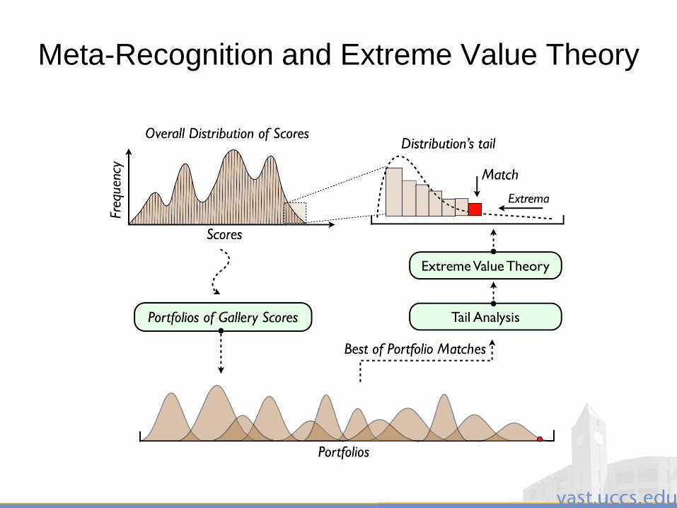
3/28/2011 240
Meta-Recognition and Extreme Value Theory
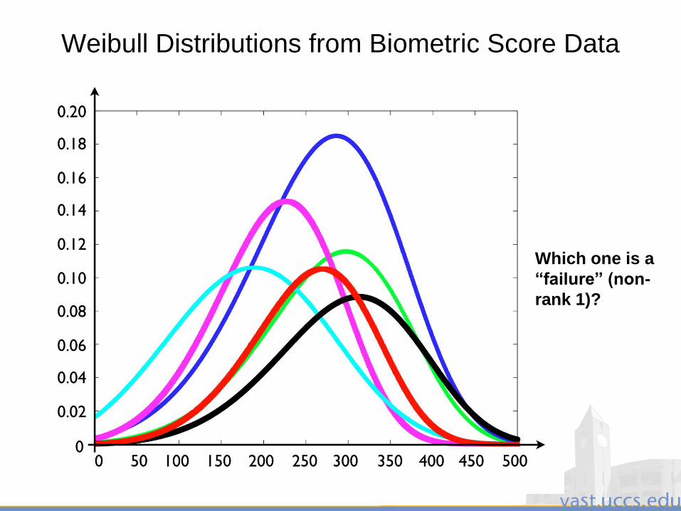
3/28/2011 241
Weibull Distributions from Biometric Score Data
Which one is a
“failure” (non-
rank 1)?
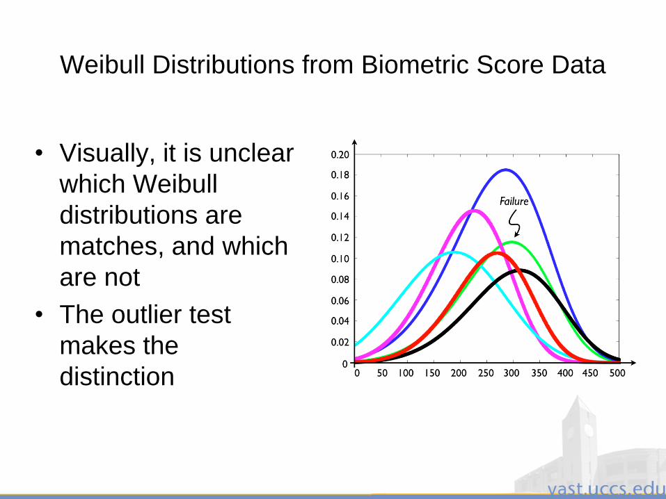
3/28/2011 242
Weibull Distributions from Biometric Score Data
• Visually, it is unclear
which Weibull
distributions are
matches, and which
are not
• The outlier test
makes the
distinction
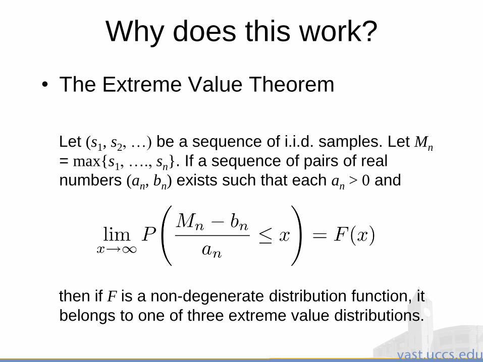
3/28/2011 243
Why does this work?
• The Extreme Value Theorem
Let (s1, s2, …) be a sequence of i.i.d. samples. Let Mn
= max{s1, …., sn}. If a sequence of pairs of real
numbers (an, bn) exists such that each an > 0 and
then if F is a non-degenerate distribution function, it
belongs to one of three extreme value distributions.

3/28/2011 244
Applying EVT to Biometric Data
• If we presume that match scores are
bounded, then the distribution of the minimum
(or maximum) reduces to a Weibull (or
Reversed Weibull)
– The sampling of the top-n scores always results in
a EVT distribution, and is Weibull if the data are
bounded.
• Generalize EVT to weaker assumption of
exchangeable random variables (as opposed
to i.i.d.)
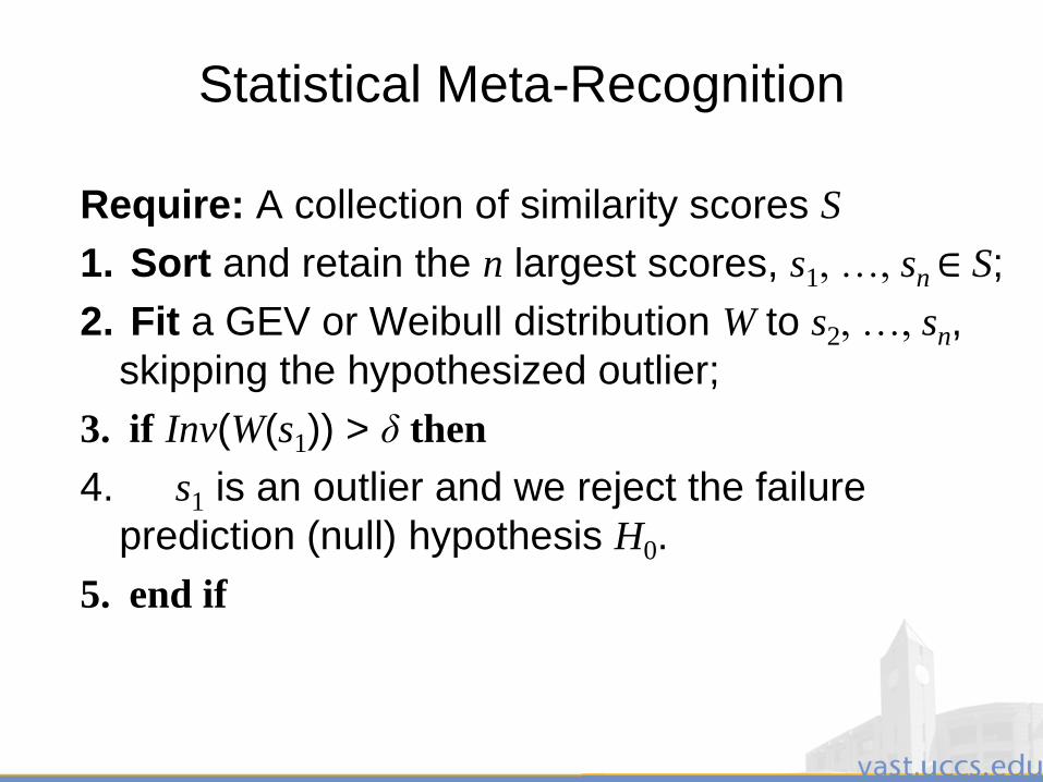
3/28/2011 245
Statistical Meta-Recognition
Require: A collection of similarity scores S
1. Sort and retain the n largest scores, s1, …, sn ∈ S;
2. Fit a GEV or Weibull distribution W to s2, …, sn,
skipping the hypothesized outlier;
3. if Inv(W(s1)) > δ then
4. s1 is an outlier and we reject the failure
prediction (null) hypothesis H0.
5. end if
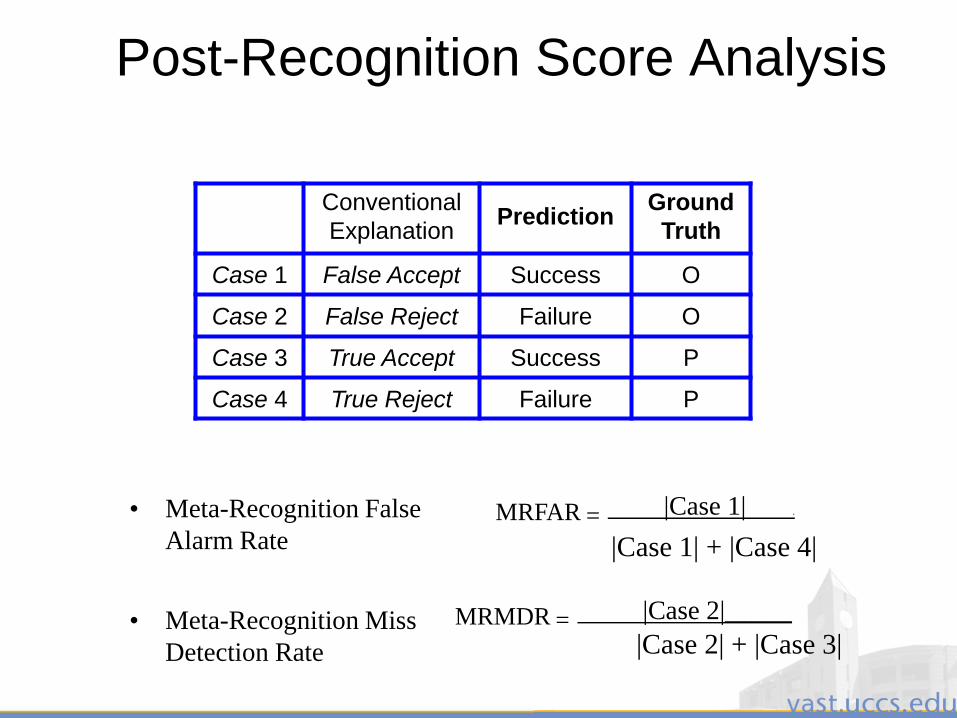
3/28/2011 246
Post-Recognition Score Analysis
• Meta-Recognition False
Alarm Rate
Conventional
ExplanationPrediction
Ground
Truth
Case 1 False Accept Success O
Case 2 False Reject Failure O
Case 3 True Accept Success P
Case 4 True Reject Failure P
MRFAR = |Case 1| .
|Case 1| + |Case 4|
MRMDR = |Case 2|_____
|Case 2| + |Case 3|• Meta-Recognition Miss
Detection Rate
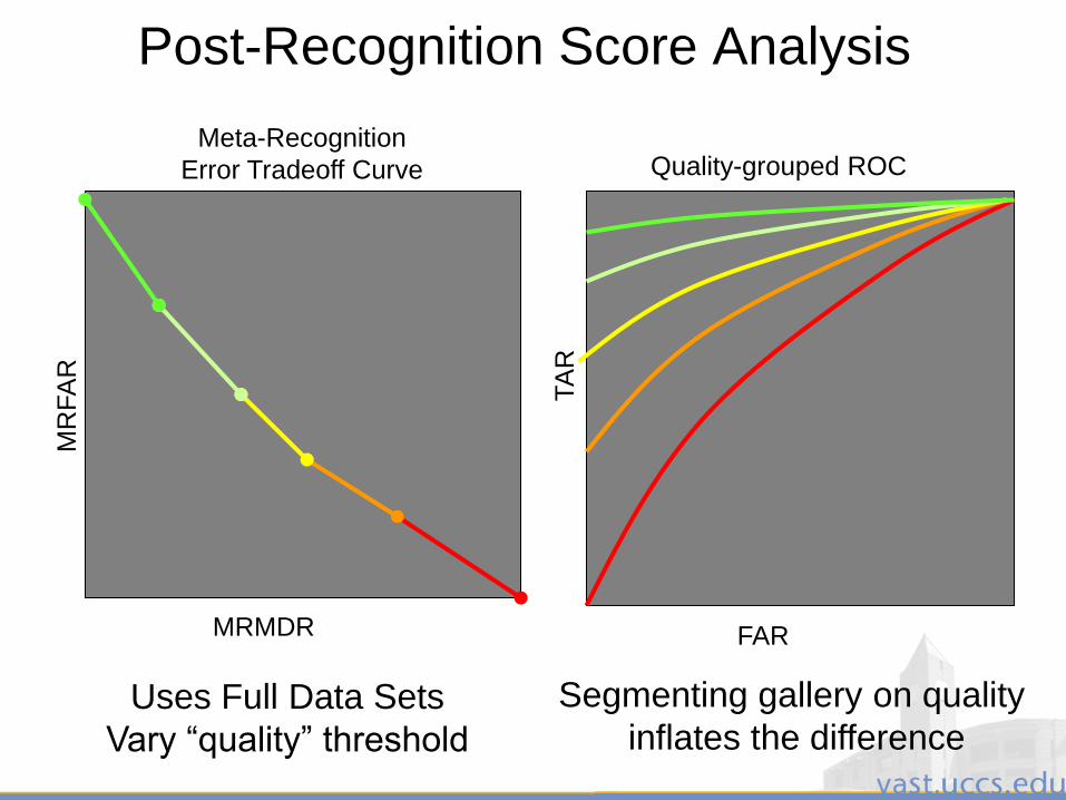
3/28/2011 247
Post-Recognition Score Analysis
MRMDR
MR
FA
R
Uses Full Data Sets
Vary “quality” threshold
FAR
TA
R
Segmenting gallery on quality
inflates the difference
Quality-grouped ROCMeta-Recognition
Error Tradeoff Curve
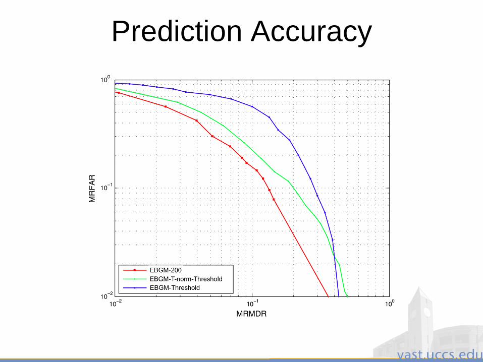
3/28/2011 248
Prediction Accuracy
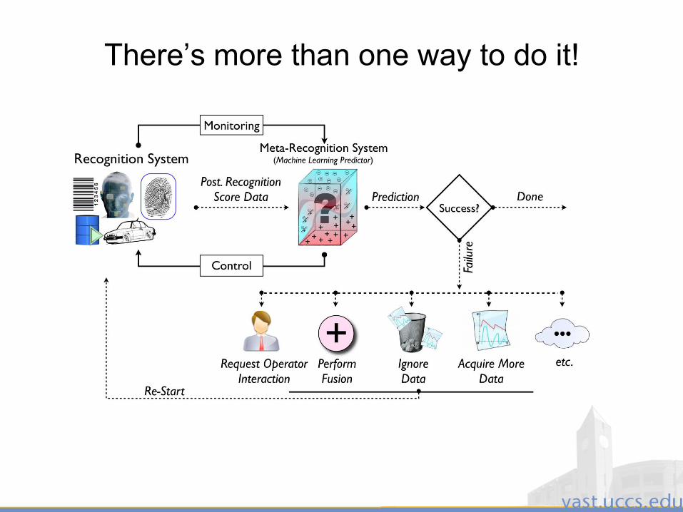
3/28/2011 249
There‟s more than one way to do it!
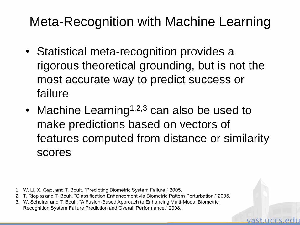
3/28/2011 250
Meta-Recognition with Machine Learning
• Statistical meta-recognition provides a
rigorous theoretical grounding, but is not the
most accurate way to predict success or
failure
• Machine Learning1,2,3 can also be used to
make predictions based on vectors of
features computed from distance or similarity
scores
1. W. Li, X. Gao, and T. Boult, “Predicting Biometric System Failure,” 2005.
2. T. Riopka and T. Boult, “Classification Enhancement via Biometric Pattern Perturbation,” 2005.
3. W. Scheirer and T. Boult, “A Fusion-Based Approach to Enhancing Multi-Modal Biometric
Recognition System Failure Prediction and Overall Performance,” 2008.
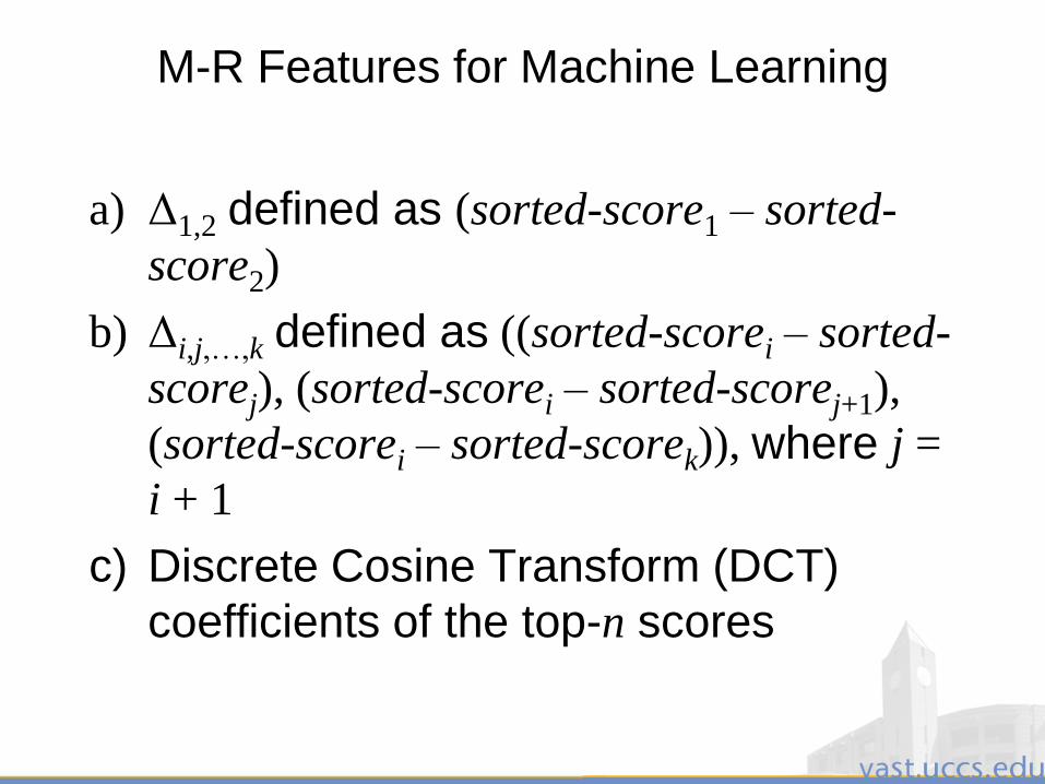
3/28/2011 251
M-R Features for Machine Learning
a) Δ1,2 defined as (sorted-score1 – sorted-
score2)
b) Δi,j,…,k defined as ((sorted-scorei – sorted-
scorej), (sorted-scorei – sorted-scorej+1),
(sorted-scorei – sorted-scorek)), where j =
i + 1
c) Discrete Cosine Transform (DCT)
coefficients of the top-n scores
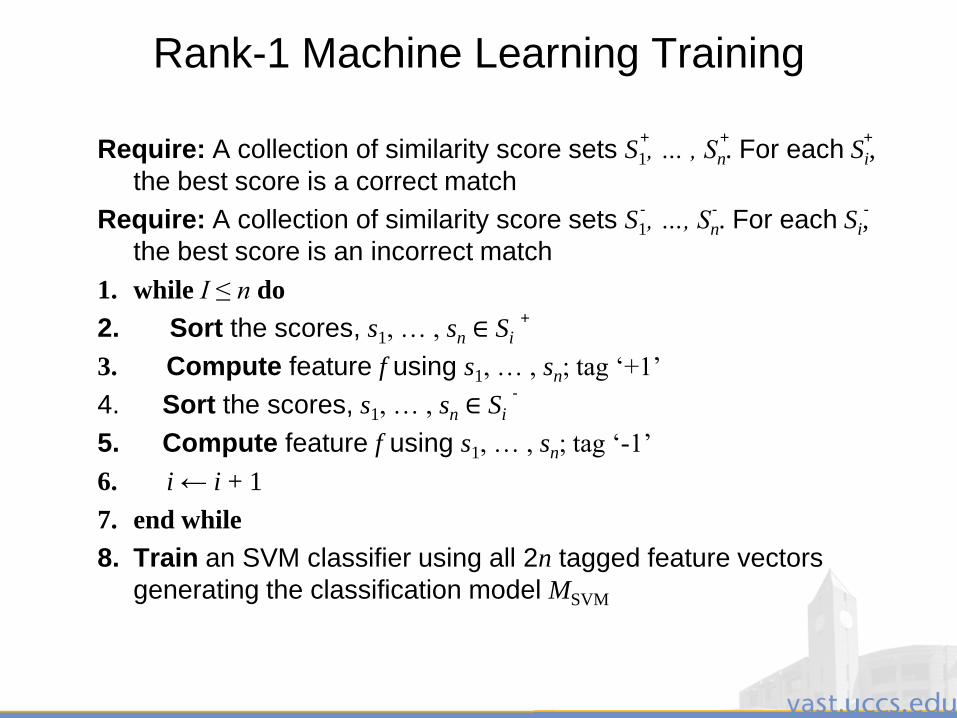
3/28/2011 252
Rank-1 Machine Learning Training
Require: A collection of similarity score sets S1, … , Sn. For each Si,
the best score is a correct match
Require: A collection of similarity score sets S1, …, Sn. For each Si,
the best score is an incorrect match
1. while I ≤ n do
2. Sort the scores, s1, … , sn ∈ Si
3. Compute feature f using s1, … , sn; tag ‘+1’
4. Sort the scores, s1, … , sn ∈ Si
5. Compute feature f using s1, … , sn; tag ‘-1’
6. i ← i + 1
7. end while
8. Train an SVM classifier using all 2n tagged feature vectors
generating the classification model MSVM
+ + +
- - -
+
-
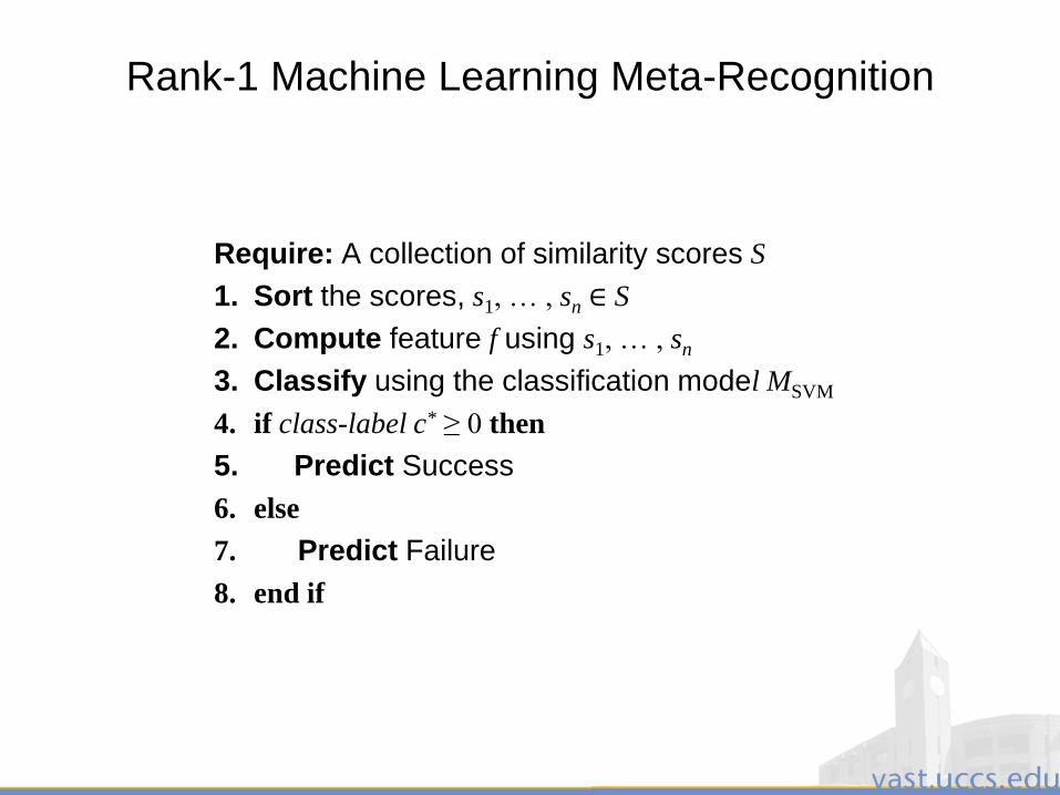
3/28/2011 253
Rank-1 Machine Learning Meta-Recognition
Require: A collection of similarity scores S
1. Sort the scores, s1, … , sn ∈ S
2. Compute feature f using s1, … , sn
3. Classify using the classification model MSVM
4. if class-label c* ≥ 0 then
5. Predict Success
6. else
7. Predict Failure
8. end if
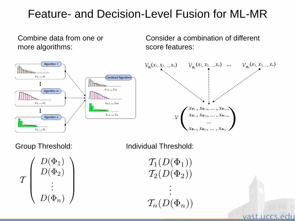
3/28/2011 254
Feature- and Decision-Level Fusion for ML-MR
Combine data from one or
more algorithms:
Consider a combination of different
score features:
Group Threshold: Individual Threshold:

3/28/2011 255
Prediction Accuracy
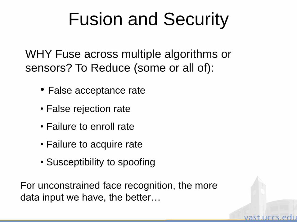
3/28/2011 256
WHY Fuse across multiple algorithms or
sensors? To Reduce (some or all of):
• False acceptance rate
• False rejection rate
• Failure to enroll rate
• Failure to acquire rate
• Susceptibility to spoofing
Fusion and Security
For unconstrained face recognition, the more
data input we have, the better…

3/28/2011 257
Biometric Fusion• Combine multiple sources of data, multiple
modalities and/or algorithms.
• Often presented as intuitive that it will improve, but must be careful not to let weak algorithms/modalities pull down good ones.
Approaches to Multi-biometric FusionMult-imodal, Multi-algorithmic, Multi-instanceMulti-sensorial, Hybrid
“Levels” of Fusion:1. Signal (Feature or Sample)
2.Score
3.Decision
3/28/2011 258
Fusion and Security
• Fusion at the matching score level (distance or
similarity scores) offers the best tradeoff in terms of
information content and application of fusion
• Empirical evaluation has indicated that a combination
approach is better than a classification approach
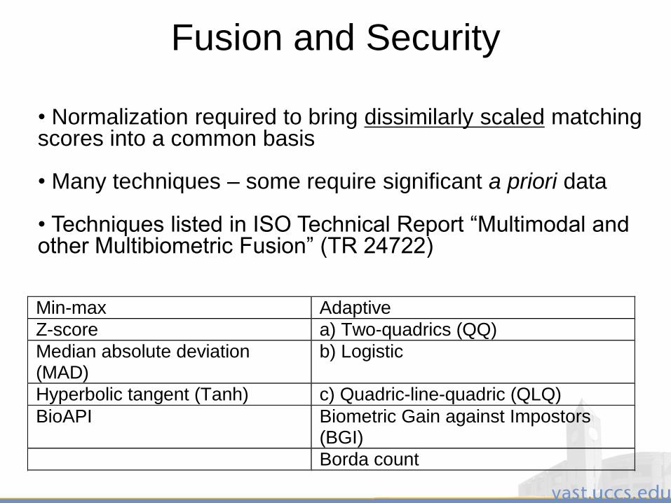
3/28/2011 259
• Normalization required to bring dissimilarly scaled matching scores into a common basis
• Many techniques – some require significant a priori data
• Techniques listed in ISO Technical Report “Multimodal and other Multibiometric Fusion” (TR 24722)
Min-max Adaptive
Z-score a) Two-quadrics (QQ)
Median absolute deviation (MAD)
b) Logistic
Hyperbolic tangent (Tanh) c) Quadric-line-quadric (QLQ)
BioAPI Biometric Gain against Impostors (BGI)
Borda count
Fusion and Security
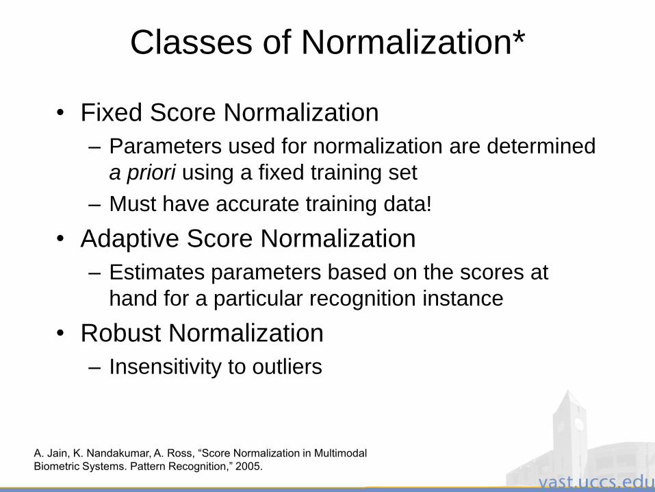
3/28/2011 260
Classes of Normalization*
• Fixed Score Normalization
– Parameters used for normalization are determined
a priori using a fixed training set
– Must have accurate training data!
• Adaptive Score Normalization
– Estimates parameters based on the scores at
hand for a particular recognition instance
• Robust Normalization
– Insensitivity to outliers
A. Jain, K. Nandakumar, A. Ross, “Score Normalization in Multimodal
Biometric Systems. Pattern Recognition,” 2005.

3/28/2011 261
• Min-max normalization: Given matching scores {sk}, k = 1, 2 , … , n the
normalized scores are given by:
• Z-score: • Median and Median Absolute Deviation (MAD):
• Double Sigmoid Function:
Fusion and Security
3/28/2011 262
More Sophisticated Fusion Approaches
• Tanh1 Estimators – fixed score normalization
that is robust to noise
– Compute “genuine score distribution” from Hampel
estimators
– Estimate mean and standard deviation from
“Genuine score distribution”
– Take the hyperbolic tangent of a z-score like
calculation
– Hampel estimators rely on ad hoc parameter
selection
*F. Hampel, P. Rousseeuw, E. Ronchetti, W. Stahel: Robust Statistics: The Approach
Based on Influence Functions. Wiley, New York (1986)
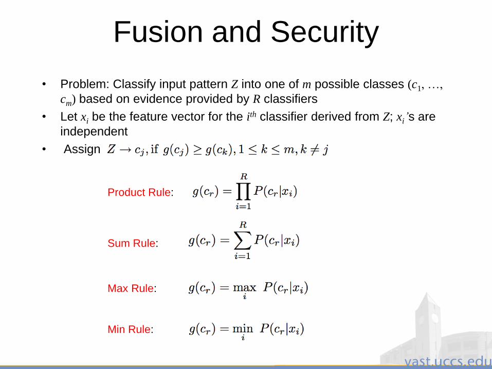
3/28/2011 263
• Problem: Classify input pattern Z into one of m possible classes (c1, …,
cm) based on evidence provided by R classifiers
• Let xi be the feature vector for the ith classifier derived from Z; xi’s are
independent
• Assign
Fusion and Security
Product Rule:
Sum Rule:
Max Rule:
Min Rule:

3/28/2011 264
Fusion Problems for
Security Watchlists
• Formal theories for existing fusion algorithms
presume consistent data and work to address
noise. What happens when user intentionally
attempts to thwart system by changing/destroying
their data.
• We need an approach to predict when a
particular modality/algorithm is failing and then
ignore it.
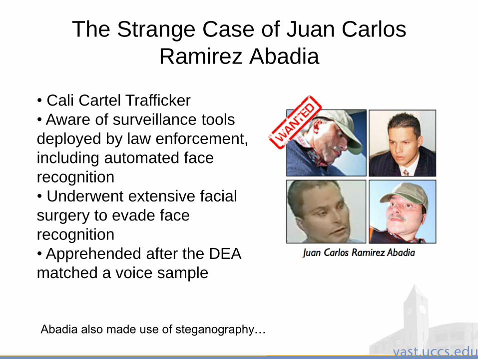
3/28/2011 265
The Strange Case of Juan Carlos
Ramirez Abadia
• Cali Cartel Trafficker
• Aware of surveillance tools
deployed by law enforcement,
including automated face
recognition
• Underwent extensive facial
surgery to evade face
recognition
• Apprehended after the DEA
matched a voice sample
Abadia also made use of steganography…
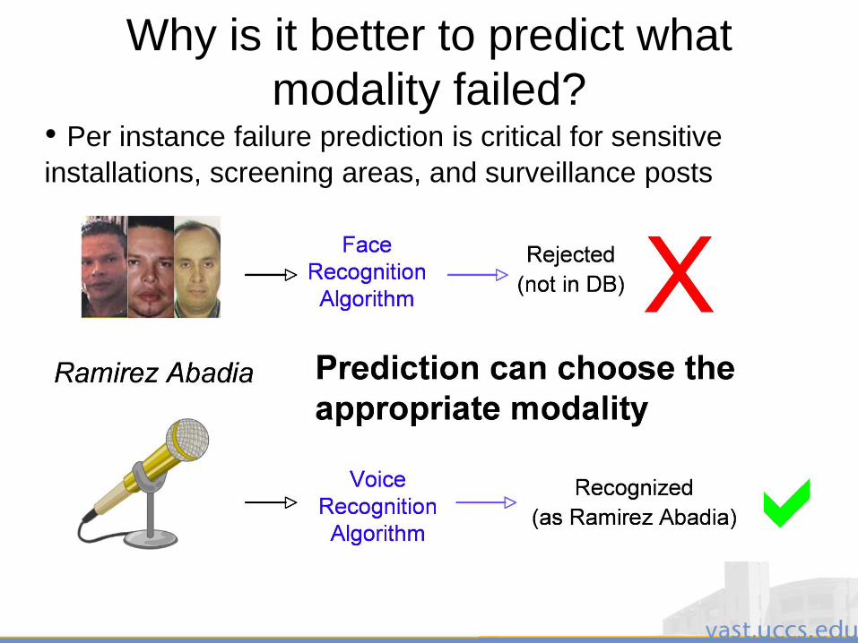
3/28/2011 266
Why is it better to predict what
modality failed? • Per instance failure prediction is critical for sensitive
installations, screening areas, and surveillance posts
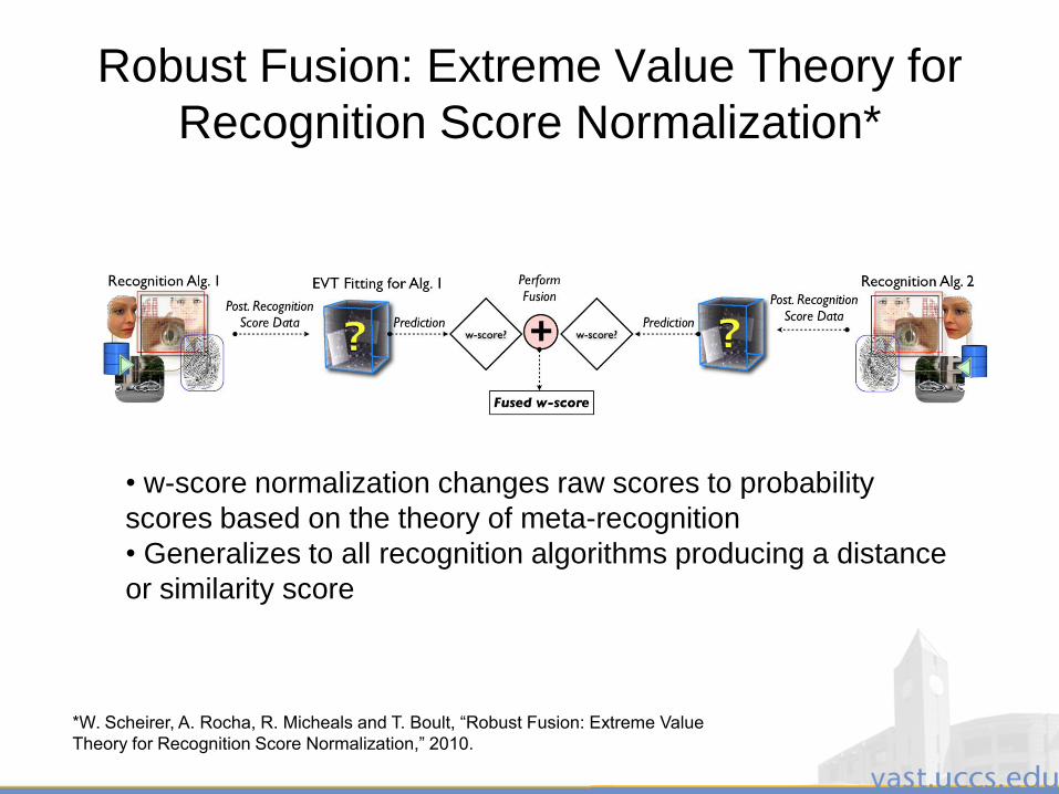
3/28/2011 267
Robust Fusion: Extreme Value Theory for
Recognition Score Normalization*
*W. Scheirer, A. Rocha, R. Micheals and T. Boult, “Robust Fusion: Extreme Value
Theory for Recognition Score Normalization,” 2010.
• w-score normalization changes raw scores to probability
scores based on the theory of meta-recognition
• Generalizes to all recognition algorithms producing a distance
or similarity score
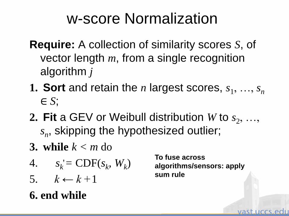
3/28/2011 268
w-score Normalization
Require: A collection of similarity scores S, of
vector length m, from a single recognition
algorithm j
1. Sort and retain the n largest scores, s1, …, sn
∈ S;
2. Fit a GEV or Weibull distribution W to s2, …,
sn, skipping the hypothesized outlier;
3. while k < m do
4. sk = CDF(sk, Wk)
5. k ← k +1
6. end while
‟To fuse across
algorithms/sensors: apply
sum rule

3/28/2011 269
w-score fusion vs. z-score sum with
failures or active imposters
3000 samples from NIST BSSR1 data
Broad
Applicability:
here we show
biometrics and
Content-based
Image Retrieval
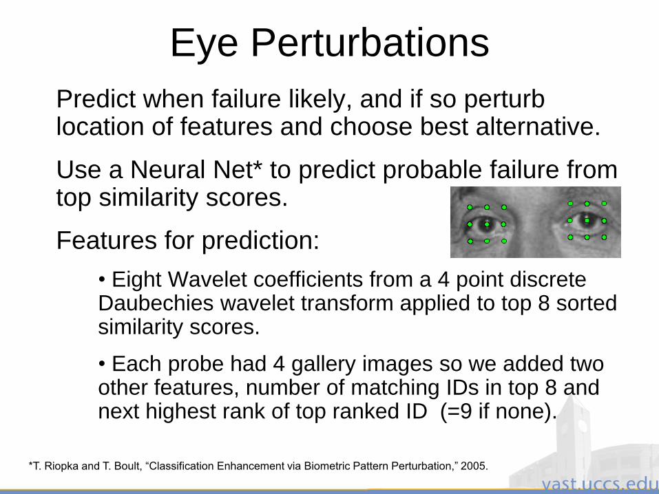
3/28/2011 270
Eye Perturbations
Predict when failure likely, and if so perturb location of features and choose best alternative.
Use a Neural Net* to predict probable failure from top similarity scores.
Features for prediction:
• Eight Wavelet coefficients from a 4 point discrete Daubechies wavelet transform applied to top 8 sorted similarity scores.
• Each probe had 4 gallery images so we added two other features, number of matching IDs in top 8 and next highest rank of top ranked ID (=9 if none).
*T. Riopka and T. Boult, “Classification Enhancement via Biometric Pattern Perturbation,” 2005.
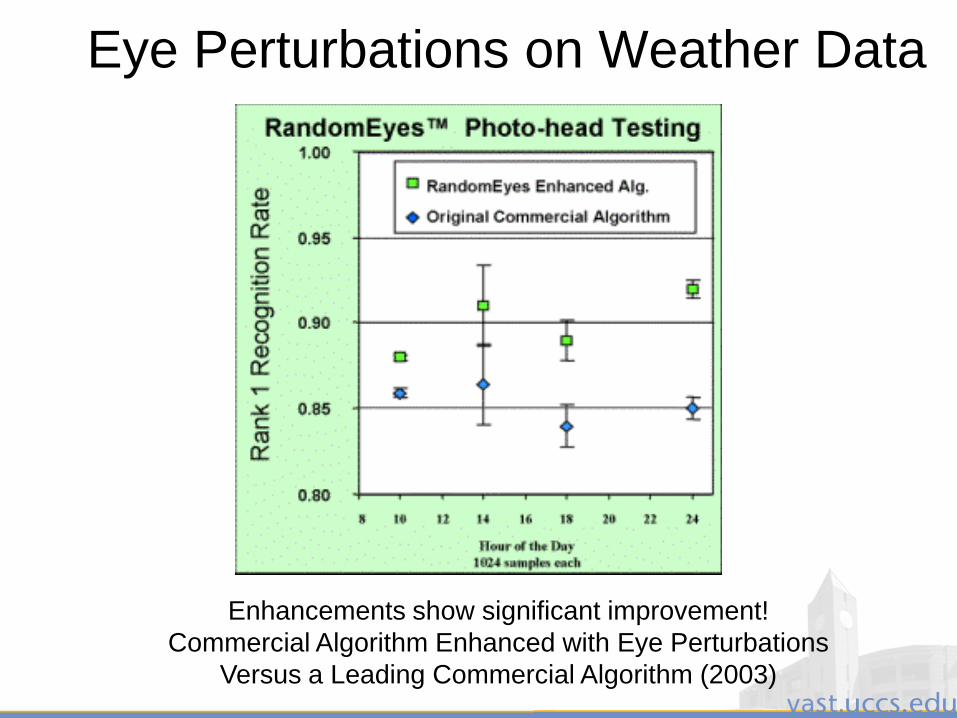
3/28/2011 271
Eye Perturbations on Weather Data
Enhancements show significant improvement!
Commercial Algorithm Enhanced with Eye Perturbations
Versus a Leading Commercial Algorithm (2003)

3/28/2011 272
New Matching Paradigm Designed to
reduce latency/processing
Long Range Image
Get Match Scores against DB
FASST prediction on score
Loop if predict FailurePredict
Fail
Long Range Image
Preprocessing: choose N pre-defined eye perturbations and
expand DB with multiple-images per subject
FASST prediction on
expanded score setFail to
match
Get Match
Scores against
Expanded DB
Match found
Match found
All
Perturbation
s Tried
Yes
Alert
Continue
Alert
Continue
Perturb eye location
and normalize Image
RandomEyes™ Search
RandomEyesDB™
Find Eyes
Find Eyes,
Normalize once
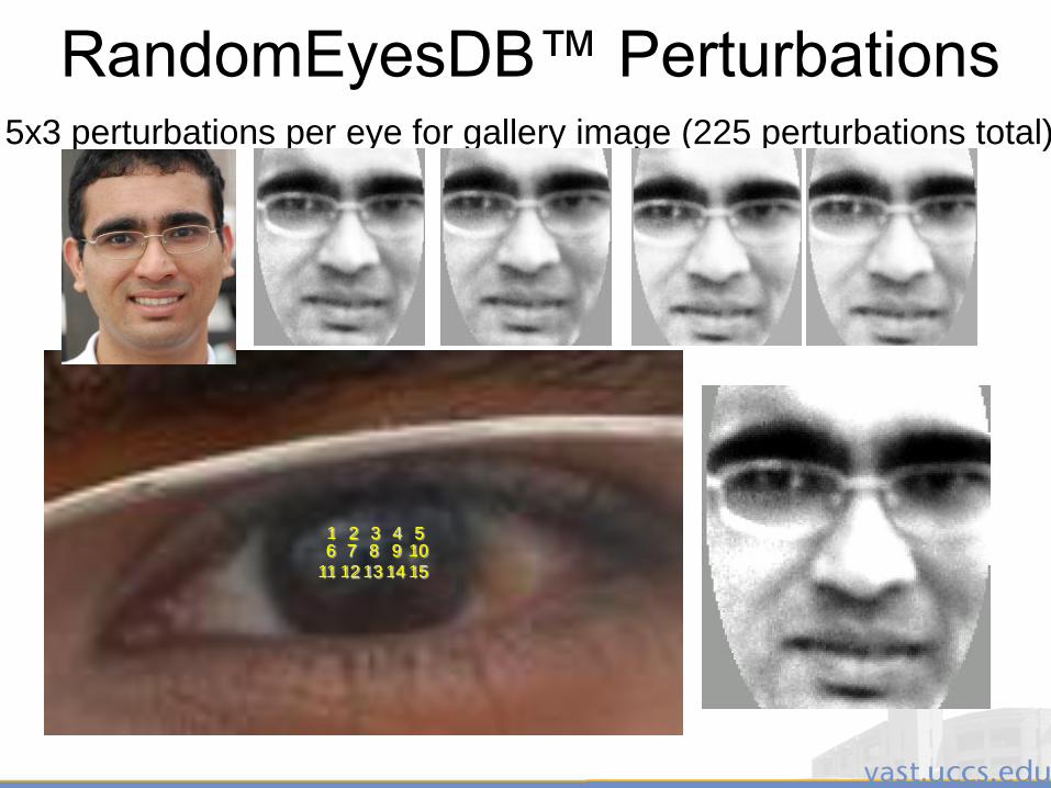
3/28/2011 273
RandomEyesDB™ Perturbations
83
72
61
94
105
131211 14 15
5x3 perturbations per eye for gallery image (225 perturbations total)

3/28/2011 274
Summary
• We are far from solving the
unconstrained face recognition problem
– Strong impact on what we can deploy
today
• Good solutions must consider all parts
of the system
– Image Acquisition, Image Enhancement,
Feature Localization, Recognition
Approach, Post-Recognition Score
Analysis
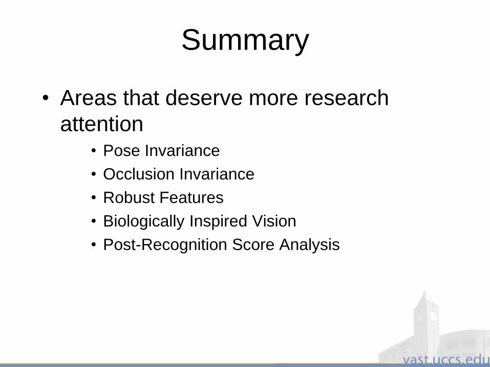
3/28/2011 275
Summary
• Areas that deserve more research
attention• Pose Invariance
• Occlusion Invariance
• Robust Features
• Biologically Inspired Vision
• Post-Recognition Score Analysis

3/28/2011 276
Thank You!
(Any final questions???)