FAA AIRPORT BENEFIT-COST ANALYSIS GUIDANCE

Office of Aviation Policy and PlansFederal Aviation Administration

December 15, 1999

iii

TABLE OF CONTENTS

Section 1: INTRODUCTION ................................................................................................. 1

1.1 Purpose of Guidance............................................................................................. 11.2 Background.......................................................................................................... 11.3 Application........................................................................................................... 11.4 Limitations of Guidance ....................................................................................... 2

Section 2: ROLE OF BCA...................................................................................................... 3

2.1 General Objectives of BCA .................................................................................. 32.2 Distinction Between BCA and Financial Analysis ................................................ 32.3 Treatment of Macro-Economic Impacts Associated with Airport Projects ............ 4

Section 3: OVERVIEW OF BCA PROCESS ........................................................................ 6

3.1 Define Project Objectives ..................................................................................... 63.2 Specify Assumptions ............................................................................................ 63.3 Identify the Base Case .......................................................................................... 63.4 Identify and Screen Reasonable Investment Alternatives ...................................... 63.5 Determine Appropriate Evaluation Period ............................................................ 63.6 Establish Reasonable Level of Effort.................................................................... 73.7 Identify, Quantify, and Evaluate Benefits and Costs ............................................. 73.8 Measure Impact of Alternatives on Airport Usage ................................................ 73.9 Compare Benefits and Costs of Alternatives......................................................... 83.10 Perform Sensitivity Analysis ................................................................................ 83.11 Make Recommendations ...................................................................................... 8

Section 4: OBJECTIVES........................................................................................................ 9

4.1 Statement of Objectives........................................................................................ 94.2 Range of Possible Objectives................................................................................ 94.3 Treatment of Multiple Objectives ......................................................................... 94.4 Designation of Principal Objective ...................................................................... 10

Section 5: ASSUMPTIONS ................................................................................................... 11

5.1 Future Airport Environment ................................................................................ 115.2 Projected Growth in Airport Activity................................................................... 115.3 Future Changes in Airport Facilities and Capacity ............................................... 135.4 Binding Constraints on Airport Capacity ............................................................. 145.5 Regional Air Traffic Management ....................................................................... 14

iv

5.6 Environmental Considerations............................................................................. 145.7 Need for New or Adjusted Assumptions.............................................................. 155.8 Economic Values.................................................................................................. 15

Section 6: IDENTIFICATION OF THE BASE CASE......................................................... 16

6.1 Need for Correct Identification ............................................................................ 166.2 Base Case Specification Requirements ................................................................ 16

Section 7: SPECIFICATION OF ALTERNATIVES ........................................................... 17

7.1 Importance of Complete Specification................................................................. 177.2 Self-contained Alternatives.................................................................................. 177.3 Range of Alternatives .......................................................................................... 17

7.3.1 Investments in New Facilities ................................................................... 177.3.2 Reconstruction of Existing Facilities......................................................... 187.3.3 Demand Management Strategies............................................................... 187.3.4 Redistribution of Responsibility................................................................ 19

7.4 Screening Alternatives......................................................................................... 19

Section 8: SELECTION OF EVALUATION PERIOD........................................................ 20

8.1 Types of Evaluation Periods ................................................................................ 208.1.1 Requirement Life...................................................................................... 208.1.2 Physical Life ............................................................................................ 208.1.3 Economic Life.......................................................................................... 208.1.4 Selection of Appropriate Time Period....................................................... 20

8.2 Comparable Time Periods For All Alternatives ................................................... 208.3 Augmentation Of Evaluation Period To Assist In Project Timing Evaluation....... 21

Section 9: LEVEL OF EFFORT ........................................................................................... 22

9.1 Appropriate Level of Effort ................................................................................. 229.2 Justification ......................................................................................................... 22

Section 10: MEASUREMENT OF BENEFITS .................................................................... 24

10.1 Benefits of Capacity Projects ............................................................................... 2410.2 Identification and Measurement of Benefits ......................................................... 2410.3 Step 1--Identification of Benefits ......................................................................... 24

10.3.1 New Airside Capacity Projects .................................................................. 2410.3.1.1 Delay Benefits .................................................................................... 27

10.3.1.2 Improved Schedule Predictability .................................................. 2710.3.1.3 More Efficient Traffic Flows ......................................................... 28

v

10.3.1.4 Use of Faster, Larger, and/or More Efficient Aircraft..................... 2810.3.1.5 Compliance with FAA Safety, Security, and Design

Standards ............................................................... 2810.3.1.6 Safety Benefits of Capacity Projects .............................................. 2910.3.1.7 Environmental Benefits of Capacity Projects ................................. 29

10.3.2 Rehabilitation of Airside Facilities ........................................................ 3010.3.3 Acquisition of Airside Equipment Supporting Capacity ........................ 3010.3.4 Airfield Safety, Security, and Design Standards Projects....................... 3010.3.5 Environmental Projects ......................................................................... 3110.3.6 Air Terminal Building Capacity Projects............................................... 3110.3.7 ATB Security Projects .......................................................................... 3110.3.8 Inter-Terminal Transportation ............................................................... 3110.3.9 Landside Access Projects ...................................................................... 32

10.4 Step 2--Measurement of Benefits ......................................................................... 3210.4.1 Analysis of Airfield Delay Reductions ................................................... 34

10.4.1.1 Airfield Simulation Models......................................................... 3510.4.1.2 Airfield Simulation Models......................................................... 3510.4.1.3 Selection of Traffic Levels for Simulation................................... 3610.4.1.4 Collection of Model Input Data................................................... 4010.4.1.5 Description of Delay ................................................................... 4210.4.1.6 Airside Passenger and Cargo Delays ........................................... 42

10.4.2 Analysis of Air Terminal Building Delay Reductions............................. 4210.4.2.1 ATB Demand.............................................................................. 4310.4.2.2 ATB Capacity ............................................................................. 43

10.4.3 Quantification of Landside Delay Reduction.......................................... 4310.4.4 Improved Schedule Predictability........................................................... 4410.4.5 More Efficient Traffic Flows.................................................................. 4410.4.6 Use of Larger, Faster and/or More Efficient Aircraft.............................. 45

10.4.6.1 Interviews with Air Service Providers ......................................... 4510.4.6.2 Passenger Surveys....................................................................... 4610.4.6.3 Analysis of Air Service at Comparable Airports.......................... 4610.4.6.4 Other Methods ............................................................................ 47

10.4.7 Safety, Security, and Design Standard Benefits Associated WithCapacity Projects...................................................................................... 4710.4.7.1 Compliance With Safety, Security, and Design Standards ........... 4710.4.7.2 Increased Safety Associated with Precision Approaches.............. 48

10.4.8 Environmental Benefits Associated With Capacity Projects .................. 4810.4.8.1 Noise Benefits............................................................................. 4810.4.8.2 Air Emissions ............................................................................. 48

10.4.9 Lower Airport Operations and Maintenance (O&M) Costs ................... 4810.5 Step 3--Valuation of Benefits............................................................................... 49

10.5.1 Constant Dollars .................................................................................... 4910.5.2 Equal Valuation of Incremental Units .................................................... 4910.5.3 Valuation of Fractional Benefit Units..................................................... 49

vi

10.5.4 Summary of Unit Values for Benefits .................................................... 5010.5.5 Valuation of Delay Reductions............................................................... 50

10.5.5.1 Valuation of Aircraft Delay Reductions....................................... 5010.5.5.2 Valuation of Passenger Delay Reductions ................................... 5410.5.5.3 Valuation of Air Cargo Delay Reductions ................................... 5410.5.5.4 Valuation of Meeter/Greeter Delay Reductions ........................... 55

10.5.6 Improved Schedule Predictability........................................................... 5510.5.7 More Efficient Traffic Flows.................................................................. 5610.5.8 Use of Larger, Faster, and/or More Efficient Aircraft ............................. 56

10.5.8.1 Lower Cost Per Revenue Mile..................................................... 5610.5.8.2 Reduced Time In Transit............................................................. 56

10.5.9 Safety, Security, and Design Standard Benefits Associated WithCapacity Projects...................................................................................... 56

10.5.10 Safety Benefits of Capacity Projects..................................................... 5610.5.11 Environmental Benefits of Capacity Projects ....................................... 5610.5.12 Airport Operating and Maintenance Benefits........................................ 57

10.6 Hard-To-Quantify Benefit and Impact Categories ................................................. 5710.6.1 Systemwide Delay ................................................................................. 5710.6.2 Increased Passenger Comfort and Convenience...................................... 5810.6.3 Non-Aviation Impacts............................................................................ 59

10.6.3.1 Macroeconomic Gains ................................................................ 5910.6.3.2 Productivity Gains ...................................................................... 60

10.7 Special Case of New Airports ............................................................................... 6110.7.1 Regional Airports .................................................................................. 6110.7.2 Replacement Airports ............................................................................ 6210.7.3 Supplemental Airports ........................................................................... 6210.7.4 Uncertainties of Traffic Forecasts at New Airports................................. 63

Section 11: COST ESTIMATION......................................................................................... 65

11.1 Costs of Capacity Projects .................................................................................... 6511.2 Cost Concepts....................................................................................................... 65

11.2.1 Opportunity Cost ................................................................................... 6511.2.2 Incremental Cost.................................................................................... 6611.2.3 Sunk Cost .............................................................................................. 6611.2.4 Depreciation .......................................................................................... 6611.2.5 Principal and Interest Expense ............................................................... 6611.2.6 Inflation ................................................................................................. 67

11.3 Life Cycle Cost Model.......................................................................................... 6711.3.1 Planning and Research and Development Cost....................................... 6711.3.2 Investment Cost ..................................................................................... 68

11.3.2.1 Land Cost ................................................................................... 6811.3.2.2 Construction Cost ....................................................................... 6811.3.2.3 Equipment, Vehicle, and Provisioning Costs ............................... 68

vii

11.3.2.4 Initial Training Cost.................................................................... 7011.3.2.5 Transition Cost ........................................................................... 70

11.3.3 Operations and Maintenance Cost (O&M) ............................................. 7011.3.3.1 Personnel Cost ............................................................................ 7011.3.3.2 Materials ..................................................................................... 7011.3.3.3 Utilities ....................................................................................... 7011.3.3.4 Recurring Travel and Transportation........................................... 72

11.3.4 Termination Cost ................................................................................... 7211.3.4.1 Dismantling Cost ........................................................................ 7211.3.4.2 Site Restoration........................................................................... 72

11.3.5 Salvage Value........................................................................................ 7211.3.6 Relationship of Cost Components .......................................................... 72

11.4 Application of Life-Cycle Costing to Facility Replacement Decisions .................. 7211.4.1 Justification for Reconstruction Projects ................................................ 7211.4.2 Consideration of Degree of Reconstruction ........................................... 73

11.4.2.1 Timing of Reconstruction............................................................ 7311.4.2.2 Degree of Reconstruction............................................................ 7311.4.2.3 Least-Cost Means of Reconstruction ........................................... 7311.4.3.4 Consideration of Linked Reconstruction Projects ........................ 74

Section 12: MULTI-PERIOD ECONOMIC DECISION CRITERIA................................. 75

12.1 Requirement for Multi-Period Analysis................................................................. 7512.2 Creation of Multi-Period Benefit Series ................................................................ 7512.3 Creation of Multi-Period Cost Series .................................................................... 7612.4 Conversion of Benefit and Cost Series to Present Value........................................ 76

12.4.1 Opportunity Cost of Money ................................................................... 7612.4.2 Inflation ................................................................................................. 7612.4.3 Risk ....................................................................................................... 77

12.5 Discount Rate ....................................................................................................... 7712.6 Basic Discounting Methodology ........................................................................... 7712.7 Alternative Evaluation Procedures ........................................................................ 78

12.7.1 Net Present Value (NPV) ....................................................................... 7812.7.2 Benefit-Cost Ratio ................................................................................. 8112.7.3 Internal Rate of Return........................................................................... 8212.7.4 Payback Period ...................................................................................... 83

12.8 Evaluation of Optimal Project Timing................................................................... 8312.9 Selection of Best Alternative................................................................................ 84

Section 13: UNCERTAINTY................................................................................................ 85

13.1 Need to Address Uncertainty ................................................................................ 8513.2 Characterizing Uncertainty ................................................................................... 8513.3 Sensitivity Analysis .............................................................................................. 85

viii

13.3.1 Probability Distributions ........................................................................ 8513.3.2 Methods of Sensitivity Analysis............................................................. 85

13.3.2.1 One Variable Test ....................................................................... 8613.3.2.2 Two Variable Test ...................................................................... 8613.3.2.3 Alternative Scenarios ................................................................... 89

Section 14: SELECTION OF OPTIMAL PROJECT .......................................................... 90

14.1 Consideration of All Information .......................................................................... 9014.2 Net Present Value ................................................................................................. 9014.3 Hard-To-Quantify Benefits and Costs ................................................................... 9014.4 Uncertainty ........................................................................................................... 90

Appendix A: TREATMENT OF INFLATION ...................................................................A-1

A.1 Introduction .........................................................................................................A-1A.2 Price Changes ......................................................................................................A-1

A.2.1 Measuring Inflation...............................................................................A-1A.2.2 Measuring Price Changes of Specific Goods and Services.....................A-3

A.3 Sources of Price Indexes ......................................................................................A-5A.3.1 General Price Level...............................................................................A-6A.3.2 Economic Sector Price Levels ...............................................................A-7A.3.3 Construction..........................................................................................A-7A.3.4 Energy ..................................................................................................A-8A.3.5 Electronics ............................................................................................A-8A.3.6 Aircraft and Parts ..................................................................................A-9

A.4 Treatment of Inflation in Benefit-Cost Analysis...............................................A-9A.4.1 Constant or Nominal Dollars.................................................................A-9A.4.2 Period Between Analysis Date and Project Start Date ......................... A-10A.4.3 Inflation During Project Life ............................................................... A-10

Appendix B: OFFICIAL GUIDANCE ON ECONOMIC ANALYSIS............................... B-1

B.1 Executive Order 12893 (January 26, 1994)........................................................... B-1B.2 OMB CIRCULAR A-94 (Revised) (October 29, 1992) ........................................ B-1B.3 Other References.................................................................................................. B-1

B.3.1 Methodological ..................................................................................... B-1B.3.2 Data Sources ......................................................................................... B-2

Appendix C: ADJUSTMENTS OF BENEFITS AND COSTS FOR INDUCED DEMAND ................................................................................................................ C-1

C.1 Consideration of Induced Demand ....................................................................... C-1C.2 Economic Framework for Estimating Benefits ..................................................... C-1

ix

C.3 Methodology to Calculate Induced Demand......................................................... C-5C.3.1 Total Trip Costs .................................................................................... C-5C.3.2 Impact of Time Savings on Trip Time ................................................... C-7C.3.3 Impact of Time Savings on Trip Fare .................................................... C-7C.3.4 Impact of Change in Total Trip Cost on Final Demand.......................... C-8

C.3.4.1 Total elasticity of Demand.......................................................... C-8C.3.4.2 Application of Total elasticity .................................................... C-9

C.4 Induced Demand at Multiple Forecast Levels..................................................... C-10C.5 Adjustments of Benefits and Costs to Reflect Induced Demand.......................... C-10

C.5.1 Benefits............................................................................................... C-11C.5.1.1 Project Versus Passenger Benefits. ........................................... C-11C.5.1.2 Benefits To Pre-Existing and Induced Traffic ........................... C-12

C.5.2 Costs................................................................................................... C-13

x

LIST OF TABLES

TABLE 5.1: Traffic Growth Assumptions............................................................................... 12TABLE 10.1: Benefits of Airport Projects................................................................................ 25TABLE 10.2: Measures of Airport Project Benefits ................................................................. 33TABLE 10.3: Impact of Induced Demand on Benefits ............................................................. 41TABLE 10.4: Valuation of Airport Project Benefits ................................................................. 51TABLE 11.1: Construction Cost Elements ............................................................................... 69TABLE 12.1: Discounting of Project Costs and Benefits.......................................................... 78TABLE 12.2: Application of NPV to Three Investment Alternatives........................................ 80TABLE 12.3: Application of Benefit-Cost Ratio Test .............................................................. 82TABLE 12.4: BCA Results for Three Alternatives................................................................... 84TABLE A.1: Gross Domestic Product Implicit Price Deflator................................................ A-2TABLE A.2: Conversion of Current Dollars to 1994 Constant Dollars................................... A-4TABLE C.1: Calculation of Induced Demand ........................................................................ C-6TABLE C.2: Total elasticity of Demand ................................................................................. C-9TABLE C.3: Impact of Induced Demand on Benefits........................................................... C-12TABLE C.4: Impact of Induced Demand on Costs............................................................... C-12

xi

LIST OF FIGURES

FIGURE 10.1: Approximation of Exponential Delay Curve ..................................................... 37FIGURE 10.2: Adjustments of Base Case Demand Forecast .................................................... 39FIGURE 11.1: Life Cycle Cost Summary ................................................................................ 71FIGURE 13.1: One Variable Uncertainty Test ......................................................................... 87FIGURE 13.2: Two Variable Uncertainty Test.......................................................................... 88FIGURE C.1: Consumer Surplus and Role of Induced Demand ............................................. C-2FIGURE C.2: Consumer Surplus with Radical Delay............................................................. C-4

1

Section 1: INTRODUCTION

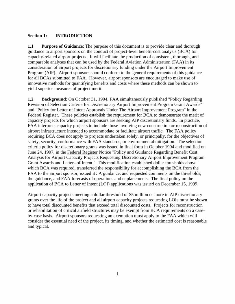
1.1 Purpose of Guidance: The purpose of this document is to provide clear and thoroughguidance to airport sponsors on the conduct of project-level benefit-cost analysis (BCA) forcapacity-related airport projects. It will facilitate the production of consistent, thorough, andcomparable analyses that can be used by the Federal Aviation Administration (FAA) in itsconsideration of airport projects for discretionary funding under the Airport ImprovementProgram (AIP). Airport sponsors should conform to the general requirements of this guidancefor all BCAs submitted to FAA. However, airport sponsors are encouraged to make use ofinnovative methods for quantifying benefits and costs where these methods can be shown toyield superior measures of project merit.

1.2 Background: On October 31, 1994, FAA simultaneously published "Policy RegardingRevision of Selection Criteria for Discretionary Airport Improvement Program Grant Awards"and "Policy for Letter of Intent Approvals Under The Airport Improvement Program" in theFederal Register. These policies establish the requirement for BCA to demonstrate the merit ofcapacity projects for which airport sponsors are seeking AIP discretionary funds. In practice,FAA interprets capacity projects to include those involving new construction or reconstruction ofairport infrastructure intended to accommodate or facilitate airport traffic. The FAA policyrequiring BCA does not apply to projects undertaken solely, or principally, for the objectives ofsafety, security, conformance with FAA standards, or environmental mitigation. The selectioncriteria policy for discretionary grants was issued in final form in October 1994 and modified onJune 24, 1997, in the Federal Register Notice "Policy and Guidance Regarding Benefit CostAnalysis for Airport Capacity Projects Requesting Discretionary Airport Improvement ProgramGrant Awards and Letters of Intent." This modification established dollar thresholds abovewhich BCA was required, transferred the responsibility for accomplishing the BCA from theFAA to the airport sponsor, issued BCA guidance, and requested comments on the thresholds,the guidance, and FAA forecasts of operations and enplanements. The final policy on theapplication of BCA to Letter of Intent (LOI) applications was issued on December 15, 1999.

Airport capacity projects meeting a dollar threshold of $5 million or more in AIP discretionarygrants over the life of the project and all airport capacity projects requesting LOIs must be shownto have total discounted benefits that exceed total discounted costs. Projects for reconstructionor rehabilitation of critical airfield structures may be exempt from BCA requirements on a case-by-case basis. Airport sponsors requesting an exemption must apply to the FAA which willconsider the essential need of the project, its timing, and whether the estimated cost is reasonableand typical.

2

1.3 Application: When possible, airport sponsors should conduct BCA as specified in thisguidance as a standard practice in the development of the airport master plan. At the master planlevel, airport sponsors should apply BCA to all capacity projects for which the sponsoranticipates the need for $5 million or more in Airport Improvement Program (AIP) discretionarygrants and for all airport capacity projects requesting LOIs.

While inclusion in a master plan appears to be the best time for BCA, other appropriateoccasions are in conjunction with environmental studies, or during project formulation. Where itis not feasible to include BCA in these activities, the BCA should be conducted on asupplemental basis and submitted to FAA when requesting funds.

FAA retains the option to review BCAs conducted by airport sponsors, request furtherdocumentation or analysis by the sponsor, and/or conduct an independent BCA.

1.4 Limitations of Guidance: FAA has attempted to present this guidance in a manner thatcovers both theoretical and practical issues of the application of BCA to airport projects. Wherepossible, a "how to" approach is provided for identifying and quantifying project benefits andcosts. However, it is impossible to define a mechanistic blueprint for BCA that would cover allpossible situations. Competent professional judgment is indispensable for the preparation of ahigh-quality analysis.

Airport sponsors and others wishing to employ BCA and evaluation techniques not covered bythis guidance should consult with the FAA Office of Aviation Policy and Plans, Systems andPolicy Analysis Division, at (202) 267-3308.

3

Section 2: ROLE OF BCA

BCA seeks to determine whether or not a certain output shall be produced and, if so, how best toproduce it. BCA requires the examination of all costs related to the production and consumptionof an output, whether the costs are borne by the producer, the consumer, or a third party.Similarly, the methods used in BCA require an examination of all benefits resulting from theproduction and consumption of the output, regardless of who realizes the benefits.

2.1 General Objectives of BCA: Benefit-cost analyses submitted to FAA should provideinformation that allows FAA to determine if:

• There is adequate information indicating the need for, and consequences of, the proposedproject or action;

• Potential benefits to society (usually defined by FAA as the aviation public) justifypotential costs (recognizing that not all benefits and costs can be described in monetary oreven in quantitative terms);

• The proposed project or action will maximize net benefits to society; and• Data used in the BCA are the best reasonably obtainable technical, economic, and other

information.

Analysis of benefits, costs, and uncertainty associated with a project or action must by guided bythe principle of full disclosure. Data, models, inferences, and assumptions should be identifiedand evaluated explicitly, together with adequate justifications for choices made, and assessmentsof the effects of these choices on the analysis.

2.2 Distinction Between BCA and Financial Analysis: BCA as discussed in this guidanceapplies to airport infrastructure investments made in whole or in part using public funds. Inparticular, AIP funds are paid from the Airport and Airway Trust Fund, which historically hasreceived its revenue from taxes imposed on aviation system users for the improvement andoperation of the airport and airway system. As such, all benefits and costs affecting the aviationpublic or directly attributable to aviation must be considered and evaluated in the BCA. Suchbenefits may include benefits realized in the form of monetary gains (e.g., lower operating costs),reductions in non-monetary resources (e.g., personal travel time), or mitigation of environmentalimpacts. A detailed listing of typical benefits and costs for inclusion in BCA studies is providedin Sections 10 and 11 of this guidance.

Airport investments to be made by a quasi-private or private entity from investment funds willgenerally be evaluated through a more restrictive form of investment evaluation known asfinancial analysis. Financial analysis considers only the cash benefits and costs accruing to thecorporation making the investment. In the case of a privately-owned airport, or a privately-owned component of a public airport, these cash benefits would principally include higher userfees (e.g., landing fees, service charges, rents, etc.) raised by the corporation from users of theairport to cover the cost of the investment.

4

It is sometimes assumed that financial analysis should be applied to publicly financed airportprojects. However, financial analysis is not appropriate because it does not measure full costsand benefits of projects to the aviation public. The following factors may cause public benefitsto vary from those captured by the project builder and operator:

• Producers sometimes create benefits for other members of the economy but are unable toobtain payment for these benefits, or alternatively may cause losses to others withouthaving to pay the full costs. These events are called externalities. A frequently citednegative externality to airport operations is aircraft noise. In the case of externalities, themeasure of net benefits to the producer will not be the same as the net benefits to thepublic.

• Public costs and benefits may not be fully captured in market transactions due toimperfect information. The full value of saved passenger time or improved air safetyattributable to an investment may not be understood by passengers and thus may bedifficult to recover through higher air fares and airport fees.

• Some airports are de facto monopoly providers of regional airport services to certainclasses of aircraft. Users of such an airport do not have reasonable alternatives to theairport should it increase its fees to cover a project's cost, although the project may ormay not have benefits equivalent to the rate increase. (Thus, the ability of an airport tocover a project's costs by a rate increase does not necessarily mean that the project haseconomic merit from the public's standpoint.)

• A project at an airport may have important benefits, but if some users are in a position toblock the project (e.g., by refusing to pay higher landing fees), the worthwhile projectcould be blocked. For instance, a dominant airline might oppose the addition of newcapacity that would disproportionately benefit its competitors, or, due to short-termfinancial problems, may reject any project with future benefits that would increasecurrent costs.

Consequently, it is appropriate that a full and objective accounting of aviation system userbenefits should be conducted through the BCA quantification methods described in thisguidance.

2.3 Treatment of Macro-Economic Impacts Associated with Airport Projects: A generalcaveat to the inclusion of benefits and costs in an airport project BCA applies to certainmacroeconomic impacts such as regional employment generation, improved businessenvironment, and other non-aviation benefits that may be generated by the project.

Macroeconomic impacts accruing to a community as a result of an airport project are difficult toquantify and frequently represent transfers from other regions. Moreover, these benefits arelargely external to the national airport system, whereas the taxes that fund the AIP are collectedfrom aviation system users to operate, maintain, and/or improve the nation's aviation system. Inaddition, Section 6(b)(3) of OMB Circular A-94 generally rules out consideration in BCAs ofemployment or output multipliers that purport to measure the secondary effects of governmentexpenditures in measured social benefits and costs.

5

However, FAA acknowledges the contributions of airports to regional economic objectives andwill consider important macroeconomic impacts separately from the BCA. A brief discussion ofmacroeconomic impacts and how they may be quantified and presented is provided in Section10.6 of this guidance.

6

Section 3: OVERVIEW OF BCA PROCESS

The BCA process consists of the following steps:

• Define project objectives• Specify assumptions about future airport conditions• Identify the base case (no investment scenario)• Identify and screen all reasonable alternatives to meet objectives• Determine appropriate evaluation period• Establish reasonable level of effort for analysis• Identify, quantify, and evaluate benefits and costs of alternatives relative to base case• Measure impact of alternatives on airport usage• Compare benefits and costs of alternatives• Evaluate variability of benefit-cost estimates• Perform distributional assessment when warranted; and• Make recommendation of best course of action

The following is a summary of the analytical considerations involved in each of these steps. Amore comprehensive discussion is provided in the remaining sections of this guidance.

3.1 Define Project Objectives: The BCA cannot proceed until the exact objectives of theproject under consideration are precisely stated. Any project undertaken without a clearunderstanding of the desired outcome is likely to be inefficient and, perhaps, unnecessary.

3.2 Specify Assumptions: A set of assumptions about the most likely future of the airportmust be explicitly stated at the outset of an analysis. These assumptions will serve as aframework for the consideration of all potential investments at the airport, and should includerealistic assessments of future traffic, traffic management improvements, constraints on futurecapacity, etc. These assumptions should be fully explained and documented.

3.3 Identify the Base Case: The base case represents the best course of action that would bepursued in the absence of a major initiative to obtain the specified objectives. The base case iscritical to BCA because it represents the reference point against which the incremental benefitsand costs of various possible investment alternatives will be measured.

3.4 Identify and Screen Reasonable Investment Alternatives: This step is one of the mostdifficult yet important parts of a BCA. It involves the identification of all reasonable ways toachieve the desired objective(s). This step is critical because only those alternatives that areidentified will be evaluated in the BCA. By definition, any alternative not identified andevaluated cannot be selected as the most efficient method to achieve the objective.

7

3.5 Determine Appropriate Evaluation Period: An unbiased comparison of investmentalternatives requires that they be analyzed over equivalent evaluation periods or time frames.Large infrastructure projects will have useful lives of 20 years or more, although for someinvestments, shorter time frames may be preferable.

3.6 Establish Reasonable Level of Effort: The amount of work and expense required toconduct a BCA can vary widely depending on:

• The importance and complexity of the project;• The number of alternatives being considered;• The availability of information on benefits and costs;• The sensitivity of net benefits to changing assumptions; and• The consequences of an incorrect decision.

The correct level of effort is a matter of judgement based on a careful assessment of these andother factors.

3.7 Identify, Quantify, and Evaluate Benefits and Costs: This step requires that the valuein dollars of all quantifiable benefits and costs be estimated for each year of the project life span.With respect to benefits, it is necessary to identify the types, amounts, and values of benefits theproject can be expected to yield. Typical benefits include reduced delay, use of more efficientaircraft, safer and more secure air travel, and reduced environmental impacts. For costs, thephysical resources consumed by the project must be determined and their associated costsestimated. Typical efforts generating costs include planning, construction, and operation andmaintenance. Guidelines for formulating benefit estimates are presented in Section 10.Procedures for cost estimation are contained in Section 11.

Not all benefits and costs can be quantified and stated in terms of dollar values. A naturalfollow-on to valuation of quantifiable benefits and costs is the identification and description ofthose benefits and costs which cannot be evaluated in dollar terms--referred to in this guidance as"hard-to-quantify". "Hard-to-quantify" considerations should be listed and described for thedecision-maker. If possible, a range in which a dollar value could be reasonably expected to fallshould be reported. Hard-to-quantify benefits and costs should not be neglected and can be veryimportant to the outcome of the analysis. These items are discussed in appropriate subsections ofSections 10 and 11.

3.8 Measure Impact of Alternatives on Airport Usage: The benefits generated by aninvestment for pre-existing airport users may induce some new users to come to the airport whowill also benefit from the project. However, these new users will impose demands on theairport's capacity that should be factored into the BCA. Appendix C of this guidance addressesthe issue of induced demand caused by airport improvements. Because of the uncertaintyassociated with the data used in an analysis of induced demand, it is left to the option of theairport sponsor whether or not to include this analysis in the BCA.

8

3.9 Compare Benefits and Costs of Alternatives: Most airport investments involve theexpenditure of large blocks of resources at the outset of the project in return for an annual flowof benefits to be realized in the future. Because benefits are not realized simultaneously withcosts, the analyst must compare total benefits and costs in a manner that recognizes that thepresent value decreases with the length of time that will occur before they are incurred. Thisprocedure establishes whether or not benefits exceed costs for any or all of the alternatives (thusindicating whether or not the objectives should be undertaken) and which alternative has thegreatest net present value. Criteria for making this comparison are enumerated in Section 12.

3.10 Perform Sensitivity Analysis: Because uncertainties are always present in the benefitand cost estimates used in the comparison of alternatives, a complete understanding of theinvestment decision can be developed only if key assumptions are allowed to vary. When this isdone, it is possible to examine how the ranking of the alternatives under consideration holds upto a change in a relevant assumption and under what conditions the project is or is not worthdoing. Methodology for conducting sensitivity analysis is presented in Section 13.

3.11 Make Recommendations: The final outcome of the economic analysis process is arecommendation concerning the proposed objective. Under a BCA there are two parts to thisrecommendation: should the activity be undertaken, and if so, which alternative should beselected to achieve it. The recommendation of the appropriate alternative will depend onmeasured benefits and costs, consideration of hard-to-quantify benefits and costs, and sensitivityof results to changes in assumptions.

9

Section 4: OBJECTIVES

4.1 Statement of Objectives: It is essential to be clear when stating the objective(s) of apotential project or action. The objective should be stated in the context of an identified problemor need at the airport. For instance, runway congestion may be causing unacceptable levels ofaircraft delay at an airport. Accordingly, the objective of the project should be stated in terms ofmitigating runway congestion to reduce aircraft delays.

The analyst should be careful not to state the project objective in a manner that prejudges themeans to obtain the objective. A runway may have reached a severe state of deterioration suchthat delays may soon be incurred due to frequent maintenance and/or closure of the runway. Inthis case, reconstruction of the runway may appear to be the obvious course of action. However,the objective of potential action should not be to "rebuild the runway to preclude thedevelopment of delay." Rather, the objective of the project should be to "undertake actions topreclude the development or worsening of airside delay." Rebuilding the runway might be onlyone of several alternatives to meet this objective.

4.2 Range of Possible Objectives: Possible objectives for an airport infrastructure projectinclude (but are not limited to) the following:

• Reduce delay associated with airport congestion;• Improve efficiency of airport operations;• Increase the number of aircraft and passengers the airport can serve;• Permit new service by accommodating larger and more efficient aircraft at the airport;• Improve (maintain) airport safety and security;• Mitigate environmental impacts of the airport on the surrounding community;• Improve passenger comfort and convenience; and• Lower airport operating costs.

4.3 Treatment of Multiple Objectives: It is likely that the project sponsor may have two (ormore) objectives and that a particular project may be able to address both. The sponsor may, forinstance, wish to reduce delay and mitigate aircraft noise--objectives that might be met by a newrunway that directs traffic over less noise-sensitive areas. However, the analyst should be carefulnot to assume that a given set of objectives must be collectively solved by one large project. Itmay be more efficient to target the various objectives with independent projects. In the aboveexample, it may prove more cost-beneficial to build a runway that does not significantlyredistribute noise but which lowers congestion, and undertake a separate noise mitigation project(e.g., noise insulation) to address the noise problem.

10

The sponsor should be especially careful not to merge separate projects designed to meetdifferent objectives into megaprojects. This practice may occur when a diverse collection ofrecommended projects (perhaps developed in an earlier master plan exercise) are presented as asingle airport development package. For instance, reconstruction and extension of a givenrunway may be marketed as one project, but in reality these are two separate projects withdifferent objectives and benefit streams. Failure to treat separate projects with differentobjectives independently could lead to incorrect decisions. The runway reconstruction mayprove cost-beneficial whereas the runway extension may not. If the projects were combined,they would either both fail or both pass--in which case a desirable project would go unbuilt or anunnecessary project would be constructed.

4.4 Designation of Principal Objective: Finally, a project undertaken for multipleobjectives must, for the purposes of AIP funding, be presented as falling principally under oneobjective. Thus, a project meeting both capacity and noise mitigation objectives must beclassified as one or the other. Project classification should conform to the principal objective ofthe project, which should also conform to the principal source of benefits stemming from theproject.

Selection of the key project objective is clearly not a matter of indifference from the standpointof this guidance. The requirement for BCA applies only to capacity-related projects funded withdiscretionary grants or LOI approvals. Due to the importance of the correct designation of thekey objective, the airport sponsor should consult with FAA at the project conception stageconcerning the specification of the key objective for any project that has any capacity-relatedbenefits.

11

Section 5: ASSUMPTIONS

5.1 Future Airport Environment: Formulating intelligent alternative courses of action toattain desired aviation objectives depends on the clear and realistic statement of assumptionsabout the future operating environment of the airport. Assumptions that should be specified anddocumented at the outset of most investment studies include:

• Projected growth in demand for airport services;• Future changes in airport facilities and capacity that are likely to occur independently of

the investment being considered;• Binding constraints on airport capacity that would not be affected by the potential

investment; and• Improvements in regional air traffic management procedures.

These and other assumptions are typically developed in the normal course of preparing an airportmaster plan.

5.2 Projected Growth in Airport Activity: Timely provision of appropriate airportinfrastructure is based on airport activity growth projections. Incorrect forecasts can lead toimproper timing of airport investments. Overly optimistic forecasts can lead to a facility being inplace far in advance of when its needed, causing scarce AIP funds to be tied up in idle facilities.Alternatively, forecasts that fail to anticipate growth may lead to unnecessary delay andinconvenience to airport users due to inadequate infrastructure. Unfortunately, realistic forecastsare difficult to make.

Chapter 5 of AC 150/5070-6A (Airport Master Plans, June 1985) provides detailed guidance onthe development of projections of the levels of growth in airside operations and enplanements atan airport. Activity forecasts are generally developed for 5, 10 and 20 year time horizons. Table5.1 summarizes the aviation demand elements that must be developed to support airport masterplanning and BCA.

Throughout this guidance, each enplanement is assumed to equal two passengers (a departureand an arrival) in the case of origin and destination (O&D) airports. At hub airports, somepassengers on continuing flights neither enplane nor deplane. A factor of 2.1 passengers perenplanement may be used at hub airports to capture through passengers.

Given the critical importance of correct forecasts on BCA results, a summary (with someaugmentation relevant to BCA) of the six step forecasting process described in AC 150/5070-6Ais provided below:

12

TABLE 5.1: TRAFFIC GROWTH ASSUMPTIONSMUST BE SPECIFIED SPECIFIED WHERE APPROPRIATENumber of Aircraft Operations (Landings and Takeoffs) Itinerant Operations Air Carrier Commuter and Air Taxi General Aviation Military

Domestic vs. International OperationsAnnual Instrument ApproachesIFR OperationsHelicopter Operations

Local Operations General Aviation Military

Touch and Go Operations

Peak Hour Operations by Aircraft TypeNumber of Passenger Enplanements Air Carrier Commuter and Air Taxi

Domestic vs. International EnplanementsGeneral Aviation EnplanementsHelicopter Enplanements

Number of Air Cargo Operations by Aircraft TypeNumber of Based Aircraft by Aircraft Type

1) Obtain existing FAA and other related forecasts for the area served by the airport beingstudied--FAA produces Terminal Area Forecasts (TAF) each year for the more than3,300 airports in the National Plan of Integrated Airport Systems. The TAF trafficprojections are based on, and controlled in aggregate by, the national FAA AviationForecast. These forecasts (which are driven by projected enplanement growth) provideenplanement and aircraft operation estimates over a future time frame for most of thecategories described in Table 5.1. State and regional aviation activity forecasts are alsoimportant sources of data, as they reflect local conditions and policy considerations.The Air Transport Association should also be consulted concerning the reasonablenessof forecasts.

2) Determine if there are significant local conditions or changes in forecast factors--FAAand other forecasts may need to be adjusted to consider local conditions not accounted forin existing forecasts. For instance, income and population levels may be growing atdifferent levels than assumed in making the forecast. In addition, planned removal of aconstraint (other than one to be addressed by the proposed investment itself) that wasspecifically factored into the existing forecast (such as night time landing restrictions)may lead to increased demand.

13

3) Make and document any adjustments to the aviation activity forecast to account for suchconditions or factors--AC 150/5070-6A describes forecast adjustment mechanisms basedon extrapolation, analysis, and judgment. All underlying assumptions, deductions, andmethods used to adjust TAF forecasts must be well-documented to facilitate FAA review.

Traffic growth estimates exceeding those in the FAA Terminal Area Forecast must beexplained or approved by FAA. Early and periodic discussions with FAA airports andforecasting staffs are encouraged.

It is critical that the basic activity forecast does not reflect any improvements associatedwith the infrastructure projects being analyzed. Methods for quantifying and evaluatinginduced activity impacts are provided in Appendix C.

4) Consider the effects of changes in uncertain factors affecting demand for the airportservices--Major components of airport demand may be driven by the continued existenceof a particular hub service or fixed base operator (FBO). Clearly, if there is a reasonablepossibility that the hub operation will be discontinued or the FBO will close down, theimpact of this event on the forecast should be quantified. Contingencies such as this mustbe specifically addressed in BCA sensitivity analysis (see Section 13).

5) Evaluate the potential for peak loads within the overall forecasts of aviation activity--It isimportant that design hour forecasts (peak hour in average month) be subjected torigorous testing of their sensitivity to the factors underlying their prediction. This isparticularly so if the design hour possesses abnormal peaking characteristics relative tothat of comparable airports. In particular, the analyst should address the likelihood ofspreading of peak demand in the event of future congestion (see Section 7.3.3). Failureto allow for adjustments to lessen peak demand in future years can lead to an over-estimation of future infrastructure needs.

6) Monitor actual activity levels over time to determine if adjustments are necessary in theforecast--Forecasts made in prior years should be monitored continuously for accuracy.Where actual traffic varies from forecast traffic, the analyst should endeavor tounderstand why this is so and make appropriate adjustments to the forecast by modifyingthe data base used to generate the forecast and/or the forecasting method. Use of aforecast made in a prior year that conflicts with recent traffic data and/or forecasts willobviously undermine the credibility of a BCA based on it.

The above six-step process focuses on growth in airside activity, but has direct applications toairport terminal building (ATB) and landside projects. In particular, airside passenger forecastscan be used to forecast passenger demand for ATB and landside facilities.

5.3 Future Changes in Airport Facilities and Capacity: The analyst must carefully outlinethe expected changes in airport conditions and capacity that are scheduled to occurindependently from the project being evaluated in the BCA. The inventory of current airport

14

plant, land use, ground access, and environmental conditions required by the master plan process(AC 150/5070-6A, Chapter 4) represents a good starting point to discuss likely changes.Development of land outside the airport's boundaries should also be addressed. Futureresidential development near an airport may greatly restrict the usefulness of a runway projectdue to noise problems.

15

A project intended to reduce runway congestion may become superfluous at some time in thefuture due to other expected development at the airport (e.g., the relocation of the airport orplanned construction of a new runway that will lead to the closure or reduced use of the currentproject). Similarly, a series of small-scale projects already approved at an airport may negate orcapture benefits being attributed to the project under consideration in the BCA. All such futuredevelopments should be listed, thoroughly discussed, and factored into the base case (see Section6).

5.4 Binding Constraints on Airport Capacity: It is rarely the case that only a singleconstraint is potentially binding on the ability of an airport to accommodate traffic growth.Therefore, a project designed to alleviate a currently binding constraint may yield benefits onlyto the point that some other constraint not addressed by the project becomes limiting.

Correct specification of potential constraints is essential to defining useful alternatives for BCAconsideration. Realization of benefits from a new runway may be contingent on simultaneousinvestments in terminal or ground access capacity. The proper identification of an alternativedesigned to capture the full potential benefit of the runway would therefore need to consider thecost of upgrading terminal or ground access capacity.

5.5 Regional Air Traffic Management: Scheduled improvements in air traffic equipmentand procedures may accomplish the same objectives that a particular infrastructure project isintended to accomplish. Such improvements may include the accommodation of higherapproach speeds, reduced separation of aircraft, redesign of airspace, and applications of newtechnologies (e.g., GPS).

Alternatively, a precision runway monitor (PRM) may permit the implementation of independentparallel approaches on runways too closely spaced for independent operations using AirportSurveillance Radar (ASR) systems. Whereas the current separation requirement without PRM is4,300 feet, it is 3,400 feet with PRM and may eventually be lowered to 2,500 feet. AC150/5070-6A (Chapter 6) discusses the issue of technology and operational improvements. FAAair traffic personnel should be consulted in the development and documentation of assumptionsconcerning the future air traffic control environment.

5.6 Environmental Considerations: The analysis should clearly address any environmentalconstraints that the airport will operate under. For instance, if the airport has an agreement withthe local community not to operate aircraft over certain areas for noise mitigation purposes, theseagreements should be explained. It would not be appropriate to attribute improved trafficpatterns to an investment when a long-term agreement precludes such traffic patterns.

On the other hand, current restraints on airport operations attributable to noise could be relaxedin the future due to the conversion of the national aircraft fleet to Stage 3 aircraft. This maypermit improvements in the utilization of current airport infrastructure and mitigate the need forthe investment in question.

16

5.7 Need for New or Adjusted Assumptions: Specification of assumptions often cannot bedone exhaustively at the initial stage of a BCA. Sufficient data may not be available to makesome assumptions up front. Other assumptions must be changed as the project proceeds andmore information is obtained or information gaps appear that can be filled only by newassumptions.

The need for revisions may become especially apparent once capacity simulation modelingbegins. For instance, should simulation modeling reveal that the baseline traffic forecast wouldlead to average airside, terminal, or landside delays of more than 20 minutes per operation orpassenger, the rate of growth in the baseline forecast would need to be adjusted downward. Thisrevision is necessary because approximately 20 minutes represents the highest level of averagedelay realized in actual practice, even at highly congested airports. A method for making suchadjustments to the basic forecast is provided in Section 10.4.1.2 of this guidance.

5.8 Economic Values: Certain economic values, also often referred to as "critical values,"are used in the conduct of BCA of investments, including capacity projects funded by AIP.These values have been collected in the document, "Economic Values for Evaluation of FederalAviation Administration Investment and Regulatory Programs," FAA-APO-98-8, dated June1998.

FAA can revise some of these values, such as aircraft capacity and utilization factors, aircraftoperating costs, and unit replacement and restoration costs of damaged aircraft. Some of thesevalues are items which the Office of the Secretary of Transportation (OST) has reserved to itselfthe right to revise, namely the value of passenger time in air travel, and the values of life andinjury in economic analysis. The discount rate is also a most critical value in BCA. The Officeof Management and Budget (OMB) has reserved to itself the right to revise the discount rate.

17

Section 6: IDENTIFICATION OF THE BASE CASE

The benefits and costs of one or more initiatives designed to accomplish specified objectivesmust be measured against a reference point, also called the base case. Ideally, the referencepoint should be the optimal course of action compatible with the specified project objectives thatwould be pursued in the absence of a major initiative. However, in most instances, the base casewill not fully meet the objectives specified for the potential project.

6.1 Need for Correct Identification: The importance of correct identification of the basecase cannot be overemphasized. If the base case is poorly designed, it will lead to incorrectestimation of the benefits and costs of the investment alternatives being considered.

It is especially important that the base case not be defined as a "do nothing" course of actionwhere the current airport configuration and management are held static. BCA based on thisstatic base case will typically overstate the deterioration in delay, efficiency, safety, and otherbenefit measures as traffic grows. In reality, airport managers, airport users, and air trafficmanagers may make a variety of operational and procedural changes to mitigate delay andrelated problems as congestion builds beyond certain thresholds.

6.2 Base Case Specification Requirements: The base case must assume optimal use ofexisting and planned airport infrastructure and incorporate all improvements to airportinfrastructure currently underway and/or funded. It must also incorporate reasonableexpectations of corrective actions by airport managers, users, and air traffic managers inresponse to build-ups in delay and other problems as airport traffic grows.

Adjustments by airport managers to accommodate congestion could include establishingvoluntary arrangements with users to spread demand outside of peak periods or offer generalaviation users incentives to use reliever facilities. Aircraft operators may make use of largeraircraft, modify schedules to take advantage of less congested periods, cancel marginal flights,etc. Reasonable assumptions about overall improvements in air traffic management should alsobe factored into the base case (see Section 5.5). All assumptions used to define the base caseshould be stated and explained.

18

Section 7: SPECIFICATION OF ALTERNATIVES

Alternatives represent the broad range of possible actions that could be undertaken to achieve theobjectives identified by the sponsor. A valid BCA must have at least one alternative identifiedfor each possible course of action. Each alternative must be a reasonable, well-founded, andself-contained investment option.

7.1 Importance of Complete Specification: It may not be possible to determine an optimalcourse of action if a full range of alternatives is not identified. In particular, any alternative notidentified and evaluated cannot, by definition, be selected as the most efficient method to achievethe objective. Therefore, an analyst should not exclude any potential alternative merely becauseof a predisposition in favor of others. Such predispositions might be due to past practice,prestige (desire to have a new or larger facility), or external constraints such as budget orpersonnel ceilings.

7.2 Self-Contained Alternatives: Each alternative should be defined so that any incrementalbenefits and costs identified for it (relative to the base case) are unambiguously and solelyattributable to it. When the realization of benefits for an alternative requires additionalinvestment in related infrastructure, the building (and cost) of this related infrastructure shouldbe included in the alternative (see Section 5.4). Only in the case where the additionalinfrastructure will be economically justified and built for reasons other than to accommodate theobjectives of the alternative could the cost of this infrastructure be excluded from the alternative.

7.3 Range of Alternatives: At a minimum, the following alternatives should be identifiedand discussed for any airport infrastructure project:

• Investments in new facilities, both major and minor, on and off the airport• Refurbishment, replacement, and enhancements of existing facilities• Demand management strategies, including provision of improved information; and• Redistribution of responsibility

7.3.1 Investments in New Facilities: One possible means to accomplish specified objectives isto build new facilities. When considering the addition of new infrastructure, a full range ofgreater and lesser investments should be addressed. For instance, a new runway could be sizedto handle all aircraft classes, or it could be sized to handle a particular class such as commuteraircraft. Similarly, a runway extension should be considered over a range of potential lengths.Each of the length alternatives would then be analyzed.

Although AC 150/5070-6A states that an airport must be designed to standards that willaccommodate the most demanding airplane (critical aircraft), the implementation of the BCArequirement for large scale projects requires that size alternatives that fall short of the designatedcritical aircraft also be considered. This requirement is particularly important when a facility isbeing expanded to accommodate a large size class of critical aircraft from what it servedpreviously. The BCA may reveal that the alternative sized to the new critical aircraft would

19

yield substantially lower net benefits than would one sized to the existing class of criticalaircraft. In this instance, FAA, in its award of grant funds, could take the position that thesmaller alternative is the preferred one even though it may not accommodate certain criticalaircraft.

In some cases, it may be logical to consider the addition of new infrastructure at a site other thanthe airport itself. If general aviation (GA) traffic is contributing to congestion at a primaryairport, construction of a new or longer GA runway at a nearby reliever airport may be a morecost-beneficial means of reducing congestion than would be the construction of a new runway atthe congested airport.

7.3.2 Reconstruction of Existing Facilities: An obvious course of action when delay or othercosts are caused by facilities in an advanced states of disrepair, obsolete equipment, or inefficientdesign is to replace the facilities or equipment. However, there may be a wide range ofalternatives to meet this course of action. Replacement can be done in place or may involvemoving the facility to another location at the airport. Reconstruction in place may range inmagnitude from partial reconstruction (e.g., removal and replacement of a layer of a runway'spavement) to full depth reconstruction (including replacement of the subgrade of the runway). Inaddition, it is appropriate to propose a range of potential enhancements that will improve on theperformance of the original. Enhancements may include strengthening (to accommodate heavieraircraft), improved materials (e.g., Portland concrete rather than asphalt concrete), better signageand lighting, etc.

7.3.3 Demand Management Strategies: FAA has generally discouraged the building of newcapacity to meet infrequent and short-lived peaks in airport traffic. One alternative forconsideration would be to encourage users of a facility to spread peak usage over a longer periodor to move usage to off-peak hours. Such inducements might include voluntary modifications toarrival and departure schedules, improvement of service at alternative airports (e.g., relieverairports), or price incentives (e.g., lower landing fees at off-peak hours). A critical role of theairport sponsor might be to provide information to airport users on the benefits associated withmovements of some flights out of the highest peak period--perhaps through a simulationmodeling exercise.

Extreme care should be exercised in the specification of any alternative to reallocate traffic byincreasing landing fees (congestion pricing) or use restrictions. Attempts to apply demandmanagement strategies at some airports have been complicated by charges that these strategieswould result in unjust discrimination against certain classes of users less able to afford higherlanding fees. However, some airports (e.g., those operated by the Port Authority of New Yorkand New Jersey) have successfully imposed congestion pricing and aircraft allocation schemesunder carefully prescribed circumstances.

20

FAA does not currently have policy guidance on implementation of fee-based demandmanagement. Until such time that a formal policy is issued by FAA, airport sponsors are advisedto consult directly with FAA (Office of Aviation Policy and Plans) prior to considering plans toimplement non-voluntary demand management strategies.

7.3.4 Redistribution of Responsibility: FAA encourages airport sponsors to consider the use ofprivate providers of infrastructure and airport services. In some cases, private providers maypossess proprietary or innovative solutions to infrastructure shortages, or they may have specialmanagement skills. When evaluating alternatives involving private provision of infrastructure,all benefits and costs to airport users should be considered, not only those benefits and costscaptured by the private provider. In addition, all AIP grant assurances associated with the airportsponsor must be honored under the terms of the contract with the private provider.

7.4 Screening Alternatives: Although as many reasonable alternatives as possible should beidentified initially, not all of these will require detailed analysis. Many technically possiblealternatives may be screened out from the beginning as inferior to others also being considered.This may occur in several situations:

• A particular approach may clearly be more costly than others, at least for the scale ofactivity under consideration;

• A particular approach may not mesh with existing facilities; and• Major political, legal, or environmental constraints may preclude implementation.

For instance, it may cost no more to replace a facility with an improvement in its design orlayout than it would cost to replace the original configuration. In this case, the originalconfiguration option would be quickly eliminated. Such determinations should be well foundedand specifically explained in the analysis.

21

Section 8: SELECTION OF EVALUATION PERIOD

8.1 Types of Evaluation Periods: The evaluation period is the number of years over whichthe benefits and costs of an investment should be considered. The choice of the evaluationperiod is dependent on the circumstances of the analysis. Three time periods are of concern indetermining the evaluation period: requirement life; physical life; and economic life.

8.1.1 Requirement Life: The requirement life is the period over which the benefits of the goodor service to be provided will be greater than the costs of producing it through the most cost-effective means. It can be for a very short period of time such as a requirement to accommodatetraffic during the reconstruction of a major airport facility. Alternatively, it may be for a verylong period of time such as the provision of a major new runway. From a practical point ofview, requirement lives should not exceed 30 years.

8.1.2 Physical Life: The physical life of an asset is that period for which the asset can beexpected to last. This period is generally not fixed--it is to a considerable degree under thecontrol of the decision-maker. Alternative facilities with different physical lives resulting frominherent quality differences can be procured or maintenance policies can be varied to alter anasset's physical life after it has been put in service.

8.1.3 Economic Life: The economic life is that period over which the asset itself can beexpected to meet the requirements for which it was acquired in a cost-effective manner. Bydefinition, economic life is less than or equal to requirement life. Economic life may equal (butnot exceed) physical life, but it is often less. If less, this indicates that it is not efficient tooperate the asset as long as possible. Rather, it would be cheaper to replace it beyond some pointin time. The need to replace often occurs as the consequence of ever rising maintenance costs,particularly for relatively old items.

8.1.4 Selection of Appropriate Time Period: Investment projects are usually evaluated overtheir economic lives. Use of the requirement life method may require the assumption that thefacilities would be replaced at the end of each economic life period forever. Such an assumption,while not improper, would add little to the analysis. Moreover, it might obscure the fact thattechnology is likely to improve with time and that better performance, lower cost alternativesmay be available in the future. To the extent that physical life exceeds economic life, it is, bydefinition, not an appropriate time period.

FAA generally uses an economic life span of 20 years beyond the completion of construction formajor airport infrastructure projects, although longer life spans may be used if justified.

8.2 Comparable Time Periods For All Alternatives: Regardless of the evaluation periodselected, it should extend over the same number of years for each alternative. This equivalenceis necessary because benefits and costs are flows that must be measured with respect to time.Clearly, if total net benefits are the basis for selection among two or more projects, net benefitsquantified over different periods will yield non-comparable results.

22

In certain situations, it will not be possible to compare alternatives with the same number of timeperiods. This situation frequently arises when an existing facility is being compared withreplacements. The existing facility will continue to be functional for some period of time,although its remaining physical life probably will not extend beyond the economic life of thenew replacement alternatives. In addition, various options being compared may have differenteconomic lives.

When the need to compare projects with different economic lives occurs, the conventionalpractice is to set the BCA timeframe to the useful life of the most durable (longest-lived)alternative. The shorter-lived alternative should be assumed to be replaced or reconstructed atthe end of its useful life so that the combined life span of the shorter-lived alternative will equalor exceed that of the longer-lived one. A residual value would then be assigned to thereplacement asset should its life exceed that of the most durable alternative. (Another approachwould be to extend the life of the shorter-lived alternative to a common timeframe with that ofthe longer-lived alternative and include the extension cost is the cost calculations. Thiseliminates the issue of salvage value, which for a government project is difficult to evaluate.)

8.3 Augmentation Of Evaluation Period To Assist In Project Timing Evaluation: FAArecommends that the selected evaluation period (e.g., 20 years) be augmented by at least 5 yearsto accommodate the need to evaluate optimal timing of investment alternatives. Inclusion of theextra 5 years will permit BCA to be completed for the specified evaluation period (20 years)beginning in year X and in year X+5. In some cases, particularly those where major benefitsdevelop late in the project's life, this process will reveal that net benefits would be maximized bywaiting to undertake an investment rather than beginning right away. A further discussion ofproject timing is provided in Section 12.

23

Section 9: LEVEL OF EFFORT

9.1 Appropriate Level of Effort: The performance of a full-fledged BCA, covering a widerange of alternatives, can be expensive and time-consuming. In certain cases that requirecomplex modeling and extensive passenger surveys, studies have required one or more years tocomplete with costs in the millions of dollars. Clearly, efforts of this magnitude would neitherbe practical nor economically justified for projects expected to cost $20 to $30 million, althoughthey may well be justified for projects expected to cost several hundred million dollars or more.

There is no exact formula for determining an appropriate or optimal level of effort. Generallyspeaking, the amount of work for an evaluation should be tailored to such things as:

• Magnitude of the project--Projects that involve major resource expenditures willgenerally require more extensive analytical efforts than will smaller, less expensiveprojects;

• Complexity of the project--Projects that have complex interactions with other airport andgroundside infrastructure may require a more extensive evaluation of total benefits andcosts;

• Number of practical alternatives--Projects involving only a limited number of reasonablealternatives will require less work than those with numerous alternatives;

• Dominance of one alternative--Level of effort can be reduced to the extent that oneoption shows a clear advantage as analysis proceeds;

• Materiality of benefits and costs--Minimal effort should be spent refining estimates ofbenefits and costs that do not vary significantly among options (base case andalternatives) or which represent a small share of the overall project benefits or cost;

• Sensitivity of benefits and costs to assumptions--Projects with important benefit and coststreams that vary greatly depending on uncertain assumptions (e.g., traffic growth)require more extensive refinements of assumptions;

• Availability of data--Projects with important benefits or costs that are inherently difficultto quantify (e.g., time savings associated with reduced congestion) will require moreeffort than those with more straightforward benefits and costs (e.g., time savingsassociated with shorter taxiing distances); and

• Controversy--Projects that are subject to large amounts of public controversy (e.g., due toenvironmental impacts) often must be investigated more thoroughly than non-controversial projects.

9.2 Justification: The BCA summary report should address how and why the specific levelof effort was selected with reference to each of the above criteria. Other considerations that maybe appropriate are the availability of time and budget to conduct the BCA. However, while lackof budget or time may constrain the scope of a BCA, they cannot be used to justify an inadequateanalysis where circumstances clearly indicate a need for more information.

Should FAA review a BCA study and conclude that the level of effort was inadequate, FAAcould require the study be redone and/or augmented. For this reason, it is highly recommended

24

that an airport sponsor consult with FAA on appropriate levels of effort before beginning full-scale analysis.

Section 10: MEASUREMENT OF BENEFITS

10.1 Benefits of Capacity Projects: The benefits that result from capacity-related airportprojects and other initiatives will largely consist of cost savings to current and future airportusers associated with reduced time spent in the airport system. Reduced time in system may takethe form of reduced delay, more efficient processing, or reduced idle time. In addition, time andcost savings can result from the ability of a facility to accommodate more efficient aircraft.Capacity-related projects may also contribute to the ability to process more operations andpassengers, greater safety and security, reduced environmental impacts, greater comfort fortravelers, and other benefits.

Measurement of benefits can be a formidable task and in some cases can only be done in aqualitative sense. However, a careful and methodical approach to benefit measurement willoften reveal that more benefits can be quantified and/or understood than was initially thoughtpossible.

10.2 Identification and Measurement of Benefits: Estimation of the total monetary value ofbenefits attributable to a project can be accomplished through a three-step identification andmeasurement process. The first step is to identify what effects will occur and who will beaffected as a consequence of undertaking an activity. The second step is to measure these effectsin physical or time-based units. Finally, the physical or time-based units must be valued indollars.

Once this three-step process is completed, the analyst can calculate the total monetary benefits tousers attributable to a project at different future traffic levels, and then determine which of thesetraffic and benefit levels corresponds most closely to final market equilibrium levels (see Section12).

10.3 Step 1--Identification of Benefits: Table 10.1 and the following text identify anddescribe the types of benefits which are often associated with various types of airside, terminal,and landside capacity-related projects. Benefits are specified with regard to whether theparticular benefit occurs to aircraft operators, passengers, or cargo shippers.

Please note that projects intended primarily to meet objectives of safety, security, designstandards, and environmental objectives are not subject to BCA requirements but are listed inTable 10.1 for the sake of completeness.

10.3.1 New Airside Capacity Projects: Airside capacity projects are intended principally toreduce airside delay, improve aircraft processing efficiency, improve predictability of landing

25

and take-off schedules, and/or to accommodate larger, heavier, longer-range aircraft at theairport. Other benefits of airfield capacity projects may include noise mitigation, reducedaircraft emissions, and compliance with FAA standards for airport safety, security, and design.

26

TABLE 10.1: BENEFITS OF AIRPORT PROJECTSPROJECT TYPE TYPICAL BENEFIT TYPEAIRSIDE

Airside Capacity Projects • New or extended runway, taxiway,

apron, or hold pad • Reduced aircraft, passenger, and cargo

delay during normal airport operations • Reduced aircraft, passenger, and cargo

delay during reconstruction of other airportfacilities

• Greater schedule predictability:- Aircraft operator able to make more

efficient use of equipment andpersonnel

- Passenger able to take later flightand arrive at destination on time

• Improved efficiency of traffic flows(reduced vectoring and taxiing distances)

• Reduced aircraft operating costs andpassenger travel times due to airport'sability to accommodate faster, larger,and/or more efficient aircraft

• Bringing pre-existing infrastructure intocompliance with FAA safety and securitystandards

• Safety improvements • Noise abatement • Reduction of aircraft emissions

• Reconstruction of runway, taxiway,apron, or hold pad

• Lower facility maintenance costs • Avoided loss of capacity benefits

associated with facility failure • Acquisition of airside equipment to

support capacity objectives(navigational aids, snow removal andmaintenance equipment)

• Reduced aircraft, passenger, and cargodelay during normal airport operations

• Greater schedule predictability • Improved safety • Lower facility maintenance costs

Airside Safety, Security, and Design Standards Projects • Installation of signage and lighting • Expansion of runway safety areas • Removal of obstructions from existing

approaches • Fencing • Acquisition of rescue and fire-fighting

equipment

• Compliance with FAR and Advisory Circularsafety, security, and design standards ismandatory and not subject to BCA.Compliance must be done in most cost-effective manner acceptable to FAA.

Airside Environmental Projects • Noise mitigation for pre-existing

infrastructure (noise insulation,structure removal)

• Fuel and chemical containment for pre-existing infrastructure

• Compliance with FAA environmental orderis mandatory and not subject to BCA.Compliance must be done in most cost-effective manner acceptable to FAA.

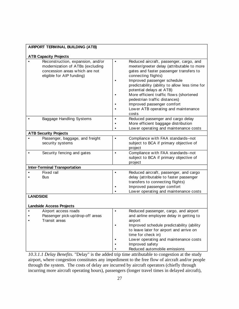
27

AIRPORT TERMINAL BUILDING (ATB)

ATB Capacity Projects• Reconstruction, expansion, and/or

modernization of ATBs (excludingconcession areas which are noteligible for AIP funding)

• Reduced aircraft, passenger, cargo, andmeeter/greeter delay (attributable to moregates and faster passenger transfers toconnecting flights)

• Improved passenger schedulepredictability (ability to allow less time forpotential delays at ATB)

• More efficient traffic flows (shortenedpedestrian traffic distances)

• Improved passenger comfort• Lower ATB operating and maintenance

costs• Baggage Handling Systems • Reduced passenger and cargo delay

• More efficient baggage distribution• Lower operating and maintenance costs

ATB Security Projects• Passenger, baggage, and freight

security systems• Compliance with FAA standards--not

subject to BCA if primary objective ofproject

• Security fencing and gates • Compliance with FAA standards--notsubject to BCA if primary objective ofproject

Inter-Terminal Transportation• Fixed rail• Bus

• Reduced aircraft, passenger, and cargodelay (attributable to faster passengertransfers to connecting flights)

• Improved passenger comfort• Lower operating and maintenance costs

LANDSIDE

Landside Access Projects• Airport access roads• Passenger pick-up/drop-off areas• Transit areas

• Reduced passenger, cargo, and airportand airline employee delay in getting toairport

• Improved schedule predictability (abilityto leave later for airport and arrive ontime for check in)

• Lower operating and maintenance costs• Improved safety• Reduced automobile emissions

10.3.1.1 Delay Benefits. "Delay" is the added trip time attributable to congestion at the studyairport, where congestion constitutes any impediment to the free flow of aircraft and/or peoplethrough the system. The costs of delay are incurred by aircraft operators (chiefly throughincurring more aircraft operating hours), passengers (longer travel times in delayed aircraft),

28

cargo shippers, and (to a limited extent) persons at the airport for purposes other than their ownair transportation needs.

Projects intended primarily to reduce airside delay include new or expanded runways, taxiways,aprons, and hold pads. These projects enable the airport to handle current or projected aircraftvolumes with less congestion, allowing larger numbers of aircraft to land, taxi, hold, and take-offin a given time period or under particular weather conditions. Aircraft flights are less likely to bedelayed (or in extreme cases, diverted or canceled), saving aircraft operators the added expenseof fuel, maintenance, and crew costs associated with delays and/or repositioning aircraft.Passengers on-board the aircraft save personal or work-related time, as may persons waiting tomeet or escort the passengers at the airport. Shippers benefit from more expedient delivery of aircargo.

In some cases, an airfield capacity project may yield only marginal delay benefits during routineairport operations, but may be critical to the airport's efficient operation during the reconstructionand temporary closure of some other component of the airport's capacity. For instance, a secondrunway can become especially important for handling traffic if the airport's primary runway mustbe closed for a prolonged period for major reconstruction.

10.3.1.2 Improved Schedule Predictability. Aircraft operators, passengers, and shippers may tie-up resources and/or pad schedules to accommodate possible delays in air travel. This risk-minimizing behavior (which effectively incorporates a delay event into a schedule whether it isrealized or not) may be particularly pronounced at airports known to have chronic or highlyvariable delays associated with airside, ATB, or landside operations.

As an example, a passenger may add half an hour to a reasonable trip time to reach an airportfrom his or her residence (due to past experience of congestion on airport roads or at airportparking facilities). The passenger may then add another 15 minutes to a reasonable time forcheck in and boarding at the ATB (due to possible expected congestion). The passenger mightalso take a flight scheduled to arrive at the destination one hour earlier than necessary (due to thelikelihood of airside departure delays and subsequent missed connections). In total, thepassenger might add an hour and 45 minutes to his or her trip even if no delays are actuallyencountered.

A capacity project can lead to delay reductions that are substantial enough to cause aircraftoperators, passengers, and shippers to place more confidence in flight and travel schedules(particularly if the project curtails the numbers of operations experiencing extreme delay events).After the project is completed, aircraft operators may reduce the amount of resources (aircraftand personnel) allocated to accommodate potential delays. Passengers travelling to time-sensitive events can take later flights and arrive at terminals closer to flight times--allowingbetter use of their time and terminal space.

Although the benefits of schedule predictability are potentially significant, it represents arelatively new category of benefit to FAA and lacks a well-tried methodology for its

29

quantification. Consequently, FAA will treat large claimed benefits from improvedpredictability with caution. However, if sufficiently large and well documented, this benefit canlend major support to an argument that a project is economically merited.

10.3.1.3 More Efficient Traffic Flows. Certain airfield improvements, including the positioningof new runways and additions of taxiways and crossovers, may permit aircraft to land, taxi, hold,and depart from an airport with reduced processing time. Reduced processing time may resultfrom reduced time spent in airborne vectoring to an open runway within the terminal airspaceand shorter taxiing distances to open runways or hold areas. These benefits would generallyresult in uncongested as well as congested conditions.

10.3.1.4 Use of Faster, Larger, and/or More Efficient Aircraft. Some capacity projects areintended primarily to accommodate faster, larger, and/or more efficient aircraft at an airport.These projects include new runways that exceed existing airport runway dimensions, andextensions to and/or strengthening of existing runways. Larger aircraft types, or current aircrafttypes carrying heavier fuel loads, can then fly directly to more distant locations (reducing routecircuits) or carry more people at lower cost on existing routes. In the case of a capacity projectthat allows an airport to accommodate jet service for the first time, passengers will alsoexperience shorter flight times to those direct destinations to be served by jet aircraft.

10.3.1.5 Compliance with FAA Safety, Security, and Design Standards. Airport capacity projectsmust conform to Federal Aviation Regulation (FAR) safety and security standards, includingFAR Part 77, "Objects Affecting Navigable Airspace," Part 107, "Airport Security," and (ifapplicable) Part 139, "Certification and Operations: Land Airports Serving Certain AirCarriers." FAA also publishes airport design and performance standards in Advisory Circular(AC) guidance, including AC 150/5300-13, "Airport Design," and AC 150/5370-10, "Standardsfor Specifying Construction of Airports." From FAA's perspective, these standards establish thebasic safety and security requirements for airport facilities, and the costs of complying with thesestandards are inherent to the minimum cost of any capacity project. No safety or security benefitcan be claimed for the potential project's conformance to FAR safety, security, and designstandards. In particular, it would be inappropriate to count as a benefit the correction of a safety,security, or design problem that would not exist if the project were not built.

Particular care should be assigned to the designation of the aircraft which will serve as thecritical (most demanding) aircraft to which the airport design must conform. FAA AC guidancedoes not mandate that a capacity and/or standards investment must be made (and funded) if aparticular critical aircraft that will serve the airport will require it. Rather, the guidance simplypresents the safety and design guidance to which the airport must conform to be served by thecritical aircraft. Consequently, the benefits associated with the airport's ability to accommodatethe critical aircraft must be sufficiently large to cover the costs of expanding the airport inconformance with FAA standards.

A benefit for compliance with FAR and AC standards compliance may be taken when a newcapacity project precludes the need to undertake remedial standards projects on pre-existing

30

infrastructure elsewhere on the airfield. For instance, a facility which was built before theissuance of current FAA standards may be used by aircraft too large to use it under the currentstandards. A new, additional facility built to FAR and AC standards and able to accommodatethe larger aircraft (which would then be excluded from the original facility) would eliminate theneed for a special project to modify the original facility.

10.3.1.6 Safety Benefits of Capacity Projects. A limited number of airfield projects intended toimprove airport capacity may have a benefit of increasing the safety of airports that alreadyoperate in full conformance with FAA safety and design standards. This safety improvement isgenerally a consequence of implementation or improvement of precision and/or reduced-obstacleapproaches and applies only to airports experiencing an overall upgrade in precision. Moreover,given the already very safe airport environment that results from compliance with FAR and ACstandards, safety benefits attributable to capacity projects will be relatively minor.

10.3.1.7 Environmental Benefits of Capacity Projects. Environmental requirements of airportcapacity and other projects are specified in FAA Order 5050.4A, "Airport EnvironmentalHandbook." The cost added to a project for compliance with this guidance must be treated as anintegral component of the cost of the new project. In general, no benefit may be attributed to theproject for compliance with the requirements of FAA Order 5050.4A because the need forcompliance would not have resulted were the project not built.

However, a capacity project may have positive environmental impacts that can be factored intothe BCA. For instance, a new runway may permit an airport to redistribute air traffic fromhighly noise-impacted areas to less noise-impacted areas. In this case, environmental benefitsmay be claimed for the noise reduction to the formerly impact area.

By reducing the time an aircraft must spend waiting in queue for take-off, an airfield capacityproject will also reduce the production of air pollutants by jet engines. In areas not in attainmentof Clean Air Act standards, this reduction can be treated as a project benefit.

31

10.3.2 Rehabilitation of Airside Facilities: Airside facilities must be periodically rebuilt orreplaced due to age, obsolescence, or premature structural failure. The critical benefit streamassociated with rehabilitation will reflect the impact on the airport if the facility were allowed tofail. Thus, for a runway, it would be appropriate to determine the impact of the runway's loss onairfield delay, schedule predictability, ability to accommodate aircraft, compliance with FAAstandards, and environmental conditions.

FAA expects that there will be relatively few situations where it will be cost-beneficial to allow amajor airside facility to fail. The more interesting problem associated with decisions onrehabilitation concern development of the most cost-effective method to accomplish it--completereconstruction, partial depth reconstruction, overlay, or intensive maintenance designed to deferthe replacement decision further into the future. It may also be appropriate to relocate therunway. Determination of replacement strategies is essentially a study of comparative costs, andthe focus of Section 11.4.

10.3.3 Acquisition of Airside Equipment Supporting Capacity: FAA is responsible for theeconomic evaluation, purchase, installation, and operation of landing and navigation aidsacquired through its airways facilities and equipment (F&E) program. In the future, AIP fundsmay be used to acquire some such systems. FAA would retain BCA responsibility for AIP-financed systems but would conduct these analyses in close cooperation with the airport sponsor.

Acquisition of snow removal, maintenance, and other miscellaneous airfield equipment is notsubject to Order 7031.2C or other FAA orders requiring BCA. Moreover, the cost of any onepurchase of this equipment will seldom cost enough to require the application of the BCAprocedure described in this guidance. In the event that a BCA must be performed, benefitswould include reduced delay (stemming from the ability to keep capacity open in inclementweather) and improved productivity of airport personnel (lower operating and maintenancecosts).

10.3.4 Airfield Safety, Security, and Design Standards Projects: FAA does not require thatinvestments or actions intended solely or principally to improve an airport's compliance withsafety, security, and design standards be subjected to BCA requirements (described in Section10.3.1.5). The principal economic requirement applying to safety, security, and designinvestments and/or actions is that they be undertaken in the most cost-effective manner possiblethat is also acceptable to FAA.1 However, were benefits of safety, security, and design standardsprojects to be measured directly in a BCA, they would include reduced fatalities, reducedinjuries, and reduced property loss or damage.

1In some cases, FAA will have already conducted program-level BCA analyses onparticular safety and security requirements, and in such cases the investmentcan be assumed to be cost-effective.

32

10.3.5 Environmental Projects: FAA does not require that investments or actions intendedprimarily to alleviate environmental problems associated with pre-existing facilities at the airportbe subjected to BCA. Rather, compliance with the requirements specified in FAA Order5050.4A must be accomplished in the most cost-effective manner possible acceptable to FAA.Were benefits of environmental (especially noise) projects to be measured directly in a BCA,they could include willingness to pay to avoid environmental degradation and avoided movingcosts.

10.3.6 Air Terminal Building Capacity Projects: Air terminal building (ATB) capacity projectsinclude new, reconstructed, or expanded ATBs, consisting of passenger halls, counter space,gates, baggage handling systems and areas, and passenger arrival and departure areas. Benefitsof these projects chiefly take the form of reduced passenger and passenger meeter/greeter delaydue to alleviation of ATB congestion, improved and/or shortened pedestrian traffic flows, andquicker unloading of passenger baggage.

Sufficient delay savings may induce some passengers to arrive at the ATB closer to actual flighttimes (rather than early to allow for potential delay), thus saving passenger time and reducingATB congestion.

ATB delay benefits may extend to aircraft operations through the availability of more gates andthe ability to transfer passengers more expeditiously between connecting flights. Other benefitsof these projects are expedited air cargo handling, lower ATB operating and maintenance costs,and improved passenger comfort and convenience.2

10.3.7 ATB Security Projects: FAA does not require that ATB investments or actionsundertaken to comply with FAA security regulations and requirements be subjected to BCA bythe airport sponsor. As in the case of airfield projects, FAA's principal economic requirement isthat the initiative represent the most cost-effective means that is also acceptable to FAA forconforming to the regulations.

10.3.8 Inter-Terminal Transportation: Larger airports with more than one ATB may undertakeprojects to expedite the movement of persons between the ATBs. Benefits of these projectsprincipally include reduced delay for passengers, passenger meeter/greeters, and airportemployees. Aircraft operators may also experience cost savings due to more efficient movementof crew members to gates and the ability to allow less time between connecting flights due toshorter inter-terminal passenger transit times.

2Concession area projects are not eligible for AIP funding. To the extentpossible, benefits (e.g., concession rents) and costs of concession projectsshould be removed from projects submitted for AIP funding.

33

10.3.9 Landside Access Projects: Efficient access to airports is vital to the perceived utility of airtransportation. Access projects, including access roads on airport property, passenger pick-upand drop-off areas, parking areas, taxi/bus marshalling areas, and acquisition of roadmaintenance equipment, may yield important benefits. These benefits might be reduced landsidedelay for passengers, meeter/greeters, cargo shippers, and airport employees attempting to get toand from the airport by automobile, bus, taxi, or rail.

Passengers, meeter/greeters, and cargo shippers using automobile or trucks will benefit fromreduced transit and vehicle hours due to less time spent in congested conditions and/or moreefficient routing. Passengers, meeter/greeters, cargo shippers, and airport and airline employeesmay also be able to schedule travel time more efficiently because they will no longer have toallow time in their schedules for potential airport road or parking congestion. Landsidecongestion may also be alleviated if persons formerly arriving early for flights are now able toarrive closer to departure times.

Other potential benefits include reduced automobile emissions (due to fewer automobiles andtrucks tied up in congested conditions), improved safety (for persons in vehicles and airportpedestrians), and lower operating and maintenance costs (due to less employee time spent incongestion while travelling on the airport grounds).

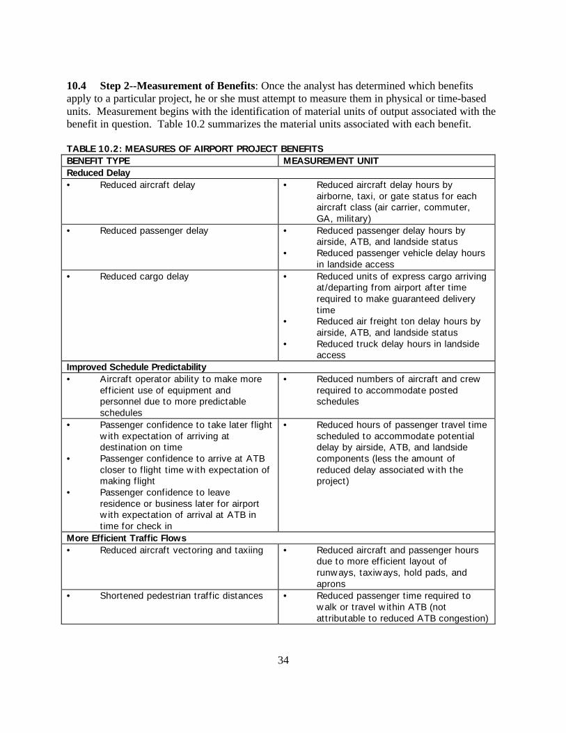
34

10.4 Step 2--Measurement of Benefits: Once the analyst has determined which benefitsapply to a particular project, he or she must attempt to measure them in physical or time-basedunits. Measurement begins with the identification of material units of output associated with thebenefit in question. Table 10.2 summarizes the material units associated with each benefit.

TABLE 10.2: MEASURES OF AIRPORT PROJECT BENEFITSBENEFIT TYPE MEASUREMENT UNITReduced Delay• Reduced aircraft delay • Reduced aircraft delay hours by

airborne, taxi, or gate status for eachaircraft class (air carrier, commuter,GA, military)

• Reduced passenger delay • Reduced passenger delay hours byairside, ATB, and landside status

• Reduced passenger vehicle delay hoursin landside access

• Reduced cargo delay • Reduced units of express cargo arrivingat/departing from airport after timerequired to make guaranteed deliverytime

• Reduced air freight ton delay hours byairside, ATB, and landside status

• Reduced truck delay hours in landsideaccess

Improved Schedule Predictability• Aircraft operator ability to make more

efficient use of equipment andpersonnel due to more predictableschedules

• Reduced numbers of aircraft and crewrequired to accommodate postedschedules

• Passenger confidence to take later flightwith expectation of arriving atdestination on time

• Passenger confidence to arrive at ATBcloser to flight time with expectation ofmaking flight

• Passenger confidence to leaveresidence or business later for airportwith expectation of arrival at ATB intime for check in

• Reduced hours of passenger travel timescheduled to accommodate potentialdelay by airside, ATB, and landsidecomponents (less the amount ofreduced delay associated with theproject)

More Efficient Traffic Flows• Reduced aircraft vectoring and taxiing • Reduced aircraft and passenger hours

due to more efficient layout ofrunways, taxiways, hold pads, andaprons

• Shortened pedestrian traffic distances • Reduced passenger time required towalk or travel within ATB (notattributable to reduced ATB congestion)

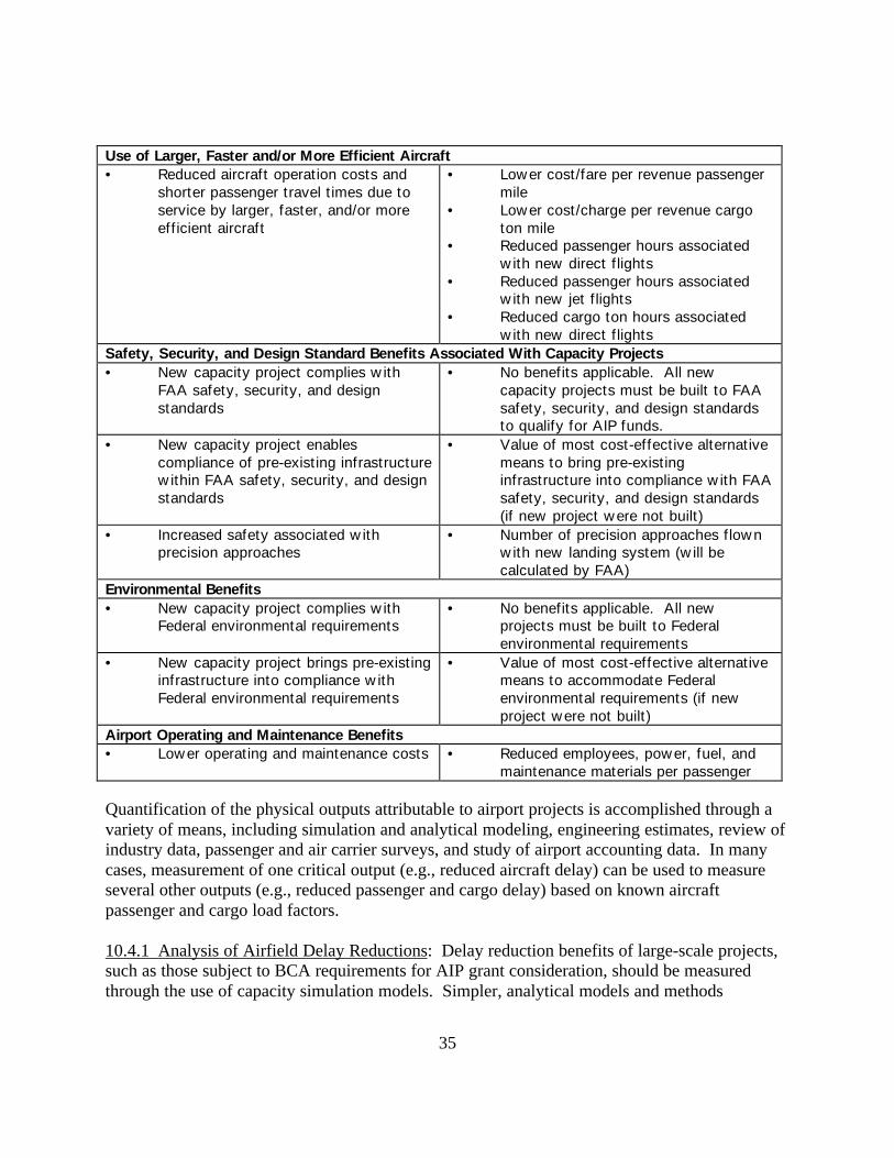
35

Use of Larger, Faster and/or More Efficient Aircraft• Reduced aircraft operation costs and

shorter passenger travel times due toservice by larger, faster, and/or moreefficient aircraft

• Lower cost/fare per revenue passengermile

• Lower cost/charge per revenue cargoton mile

• Reduced passenger hours associatedwith new direct flights

• Reduced passenger hours associatedwith new jet flights

• Reduced cargo ton hours associatedwith new direct flights

Safety, Security, and Design Standard Benefits Associated With Capacity Projects• New capacity project complies with

FAA safety, security, and designstandards

• No benefits applicable. All newcapacity projects must be built to FAAsafety, security, and design standardsto qualify for AIP funds.

• New capacity project enablescompliance of pre-existing infrastructurewithin FAA safety, security, and designstandards

• Value of most cost-effective alternativemeans to bring pre-existinginfrastructure into compliance with FAAsafety, security, and design standards(if new project were not built)

• Increased safety associated withprecision approaches

• Number of precision approaches flownwith new landing system (will becalculated by FAA)

Environmental Benefits• New capacity project complies with

Federal environmental requirements• No benefits applicable. All new

projects must be built to Federalenvironmental requirements

• New capacity project brings pre-existinginfrastructure into compliance withFederal environmental requirements

• Value of most cost-effective alternativemeans to accommodate Federalenvironmental requirements (if newproject were not built)

Airport Operating and Maintenance Benefits• Lower operating and maintenance costs • Reduced employees, power, fuel, and

maintenance materials per passenger

Quantification of the physical outputs attributable to airport projects is accomplished through avariety of means, including simulation and analytical modeling, engineering estimates, review ofindustry data, passenger and air carrier surveys, and study of airport accounting data. In manycases, measurement of one critical output (e.g., reduced aircraft delay) can be used to measureseveral other outputs (e.g., reduced passenger and cargo delay) based on known aircraftpassenger and cargo load factors.

10.4.1 Analysis of Airfield Delay Reductions: Delay reduction benefits of large-scale projects,such as those subject to BCA requirements for AIP grant consideration, should be measuredthrough the use of capacity simulation models. Simpler, analytical models and methods

36

described in FAA AC 150/5060-5, "Airport Capacity and Delay") should be used only insituations that are well understood and/or uncomplicated.

10.4.1.1 Airfield Simulation Models. Airfield simulation models are queuing models that acceptas inputs a series of events (airline and other flight schedules) and measure the flow of theseevents through a system with defined processing and performance capabilities (i.e., airfield andair traffic capacity). Arrivals and departures are linked in the schedule and are recognizeddynamically. The models estimate aircraft operational delay as a function of demand in excessof processing capability.

Airfield simulation models vary in sophistication and computational requirements, depending onthe range of factors, detail, and scope of the operating environment considered by the model.Sophisticated airfield models are time-consuming and expensive to operate. In general, thechoice of a model should conform to the complexity and cost of the project. Projects with majorimpacts on regional airspace or which would cost $50 million should be modeled using moresophisticated simulation models (see Section 9 on level of effort).

FAA makes use of three simulation models for its airfield capacity analyses. These models arethe FAA Airport and Airspace Simulation Model (SIMMOD), the Airfield Delay SimulationModel (ADSIM), and the Runway Delay Simulation Model (RDSIM). Of these, SIMMOD isthe most complex. It considers airspace and airports in a selected geographical area (multi-airport configurations can be studied) and is capable of calculating delay impacts of a variety ofoperating alternatives, including different runway configurations, air routes, sectorization, andaircraft separation standards. A SIMMOD analysis generally requires several months in order toaccomplish data collection, model specification, model runs, and interpretation of results.3

ADSIM calculates travel time, delay, and flow rate data to analyze operations at an airport andits adjacent airspace. An ADSIM analysis can generally be completed in two months or less.RDSIM is a sub-component of ADSIM that focuses only on an airport's final approach, runway,and runway exit. Analysis using RDSIM can often be completed in a matter of weeks.Information concerning all three of the above simulation models is available to the publicthrough the FAA Technical Center. In addition, a growing number of proprietary models (manyof which would be acceptable to FAA upon prior consultation) are also available and may beused.

10.4.1.2 Capacity Simulation Models. At a minimum, FAA acceptance of capacity simulationresults is contingent on the analyst demonstrating that the following objectives were achieved:

• Estimation of realistic values for performance rates at the study airport;• Analysis and determination of the interaction between arrival and departure rates;• Measurement of airport performance under different weather conditions;• Prediction of airport operational capacity; and 3See "SIMMOD User Manual," Release 1.2, March 1991.

37

• Evaluation of optimal airport capacity utilization.

10.4.1.3 Selection of Traffic Levels for Simulation. Delay reductions attributable toimprovements in infrastructure are measured by first simulating average delays associated withprojected traffic levels for the base case. Traffic levels are input into the model as aircraftoperations.

Projections of base case traffic should be taken from the FAA TAF or some other FAA-approvedforecast (see Section 5.2) which links the traffic levels with specific future years. At least threetraffic levels should be simulated initially--one typical of the beginning of the project'soperational life, one from the middle point of the project's operational life, and one from a year ator near the end of project's life. These selected traffic levels generally define the focus years forall project analysis. Intermediate years are generally approximated by interpolation and/orextrapolation.4

Simulation runs at each demand level should be conducted for representative weather conditionsand runway configurations, and then annualized to yield average delay per operation over thecourse of a year. After completion of simulation analysis on the base case scenario, theparameters of the simulation model are adjusted to reflect the improvement in capacityassociated with the investment alternative and the simulation is run again at the same trafficlevels. Average delay per operation associated with the project alternative should be subtractedfrom delay associated with the base case to determine net delay savings attributable to thealternative being evaluated.

Simulation of Additional Traffic Levels. Simulation analysis of more than three futuretraffic levels may be required if traffic and/or delay are expected to grow rapidly. Inclusion of afourth traffic level (usually intermediate to the middle and end levels initially tested) isparticularly important if simulation analysis reveals that delay begins to grow exponentiallybeyond some level of demand which can reasonably be expected to occur.

Average delay estimated by simulation models usually builds gradually over some range offuture operations growth and then may begin to mount rapidly as the extreme limits of theairport's capability are approached and exceeded. Plotted average delay curves where airportcapacity has been exceeded should conform to the curvilinear trend shown in Figure 10.1.However, approximation of this curve by connecting the average delay estimates for the basecase in years A, B, and C yields a poor approximation of the true delay trend. Inclusion of afourth focus year, D, enables a much better linear approximation of the true curve.

4Due to the expense involved in simulation modeling, it is generally notpractical to model every year of the project's operating life.

38

DelayPerOperat ion

Year

Figure 10.1: Approximation of Exponential Delay Curve

1998 2007 20152012

Overstated Delay in 2012

New Traffic Level

AB

D

C

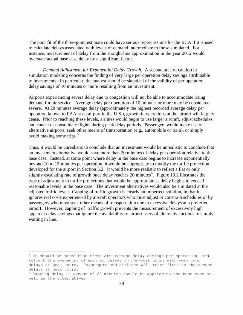
39

The poor fit of the three-point estimate could have serious repercussions for the BCA if it is usedto calculate delays associated with levels of demand intermediate to those simulated. Forinstance, measurement of delay from the straight-line approximation in the year 2012 wouldoverstate actual base case delay by a significant factor.

Demand Adjustment for Exponential Delay Growth. A second area of caution insimulation modeling concerns the finding of very large per operation delay savings attributableto investments. In particular, the analyst should be skeptical of the validity of per operationdelay savings of 10 minutes or more resulting from an investment.

Airports experiencing severe delay due to congestion will not be able to accommodate risingdemand for air service. Average delay per operation of 10 minutes or more may be consideredsevere. At 20 minutes average delay (approximately the highest recorded average delay peroperation known to FAA at an airport in the U.S.), growth in operations at the airport will largelycease. Prior to reaching these levels, airlines would begin to use larger aircraft, adjust schedules,and cancel or consolidate flights during peak delay periods. Passengers would make use ofalternative airports, seek other means of transportation (e.g., automobile or train), or simplyavoid making some trips.5

Thus, it would be unrealistic to conclude that an investment would be unrealistic to conclude thatan investment alternative would save more than 20 minutes of delay per operation relative to thebase case. Instead, at some point where delay in the base case begins to increase exponentiallybeyond 10 to 15 minutes per operation, it would be appropriate to modify the traffic projectiondeveloped for the airport in Section 5.2. It would be more realistic to reflect a flat or onlyslightly escalating rate of growth once delay reaches 20 minutes6. Figure 10.2 illustrates thetype of adjustment to traffic projections that would be appropriate as delay begins to exceedreasonable levels in the base case. The investment alternatives would also be simulated at theadjusted traffic levels. Capping of traffic growth is clearly an imperfect solution, in that itignores real costs experienced by aircraft operators who must adjust or constrain schedules or bypassengers who must seek other means of transportation due to excessive delays at a preferredairport. However, capping of traffic growth prevents the measurement of excessively highapparent delay savings that ignore the availability to airport users of alternative actions to simplywaiting in line.

5 It should be noted that these are average delay savings per operation, andreflect the averaging of minimal delays in non-peak hours with very longdelays at peak hours. Passengers and airlines will react first to the excessdelays at peak hours.6 Capping delay in excess of 20 minutes should be applied to the base case aswell as the alternatives

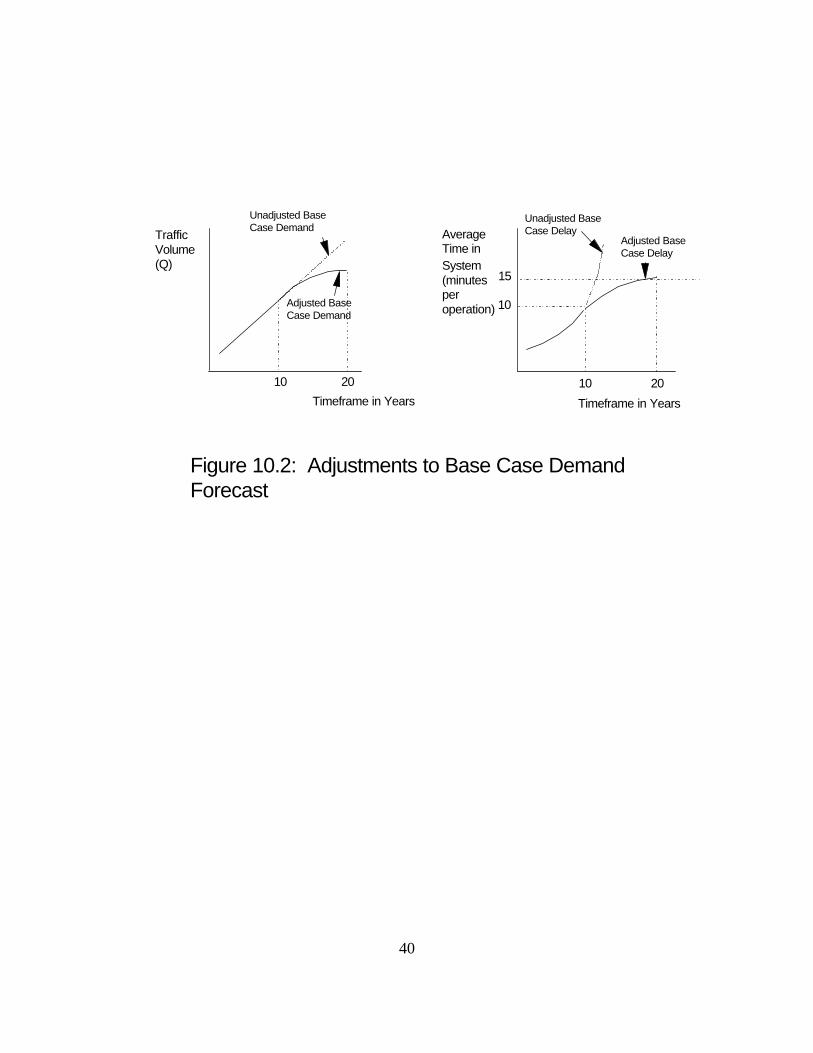
40

Figure 10.2: Adjustments to Base Case Demand Forecast

Traffic Volume (Q)

Timeframe in Years

10 20

Average Time in System (minutes per operation)

Timeframe in Years

10 20

Unadjusted Base Case Demand

Adjusted Base Case Demand

Unadjusted Base Case Delay

Adjusted Base Case Delay

10

15

41

Allowance for Induced Demand. It is often the case with transportation projects that animprovement in service attributable to an investment at a facility will induce greater use of thefacility than would have occurred without the investment. For instance, an investment thatlowers average delay at an airport will induce some potential customers who formerly avoidedthe airport to use it. However, these additional users will place new demands on the facility andmay to some extent erode the per operation delay savings to pre-existing airport users.

Although the phenomenon of "induced demand" is real, due to uncertainty in the data, itsanalysis is at the airport sponsor's option in the BCA and is the subject of Appendix C of thisguidance. However, it is important when doing capacity simulations to anticipate the needs fordata for calculating induced demand. Consequently, when preliminary simulation analysisreveals a significant delay saving attributable to an investment alternative, FAA recommendsthat the level of traffic associated with this delay result be adjusted upwards by small percentageincrements and the model re-estimated at the augmented traffic levels. The following generalguidance should be followed for deciding when incremental traffic adjustments may beappropriate:

• For projects where delay savings are expected to constitute the majority of projectbenefits, no adjustments to the simulated traffic level need be made when average delaysavings associated with the project are 1 minute per operation or less. Time savings ofthis magnitude will generally not be sufficient to induce significant numbers of newpassengers to use the airport relative to the base case traffic assumption.

• If other benefits besides delay reductions are expected to be prominent project benefitsand/or if delay savings are more than one minute per operation, it is advisable to re-simulate the project alternative case assuming 2 percent increments inoperations/passengers. As a rule of thumb, one 2 percent increment to base case demandshould be simulated for the project case for each 3 minute saving attributable to theproject. Thus, in the case of a project saving 6 minutes per operation relative to the basecase, demand levels equivalent to the base case demand, the base case demand plus2 percent, and the base case demand plus 4 percent should be simulated for the projectcase.

Resulting delays should be recorded and contrasted to the delays of the base case, as shown inthe example of Table 10.3. Appendix C presents a detailed methodology for interpreting the datacollected in Table 10.3.

10.4.1.4 Collection of Model Input Data. Data used to specify simulation models are taken fromvarious sources. Larger airports can take advantage of FAA's Enhanced Traffic ManagementSystem (ETMS), which includes information on arrival (AZ), departure (DZ), and other Zmessages. Other data sources include surface observation weather data, data provided by airtraffic controllers, and data from airports on runway configurations (log records from someairports).

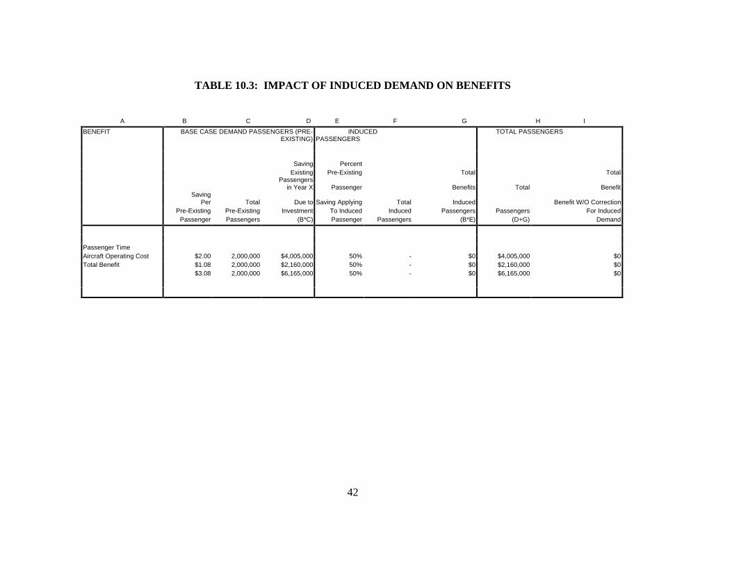
42

TABLE 10.3: IMPACT OF INDUCED DEMAND ON BENEFITS

A B C D E F G H I

BENEFIT BASE CASE DEMAND PASSENGERS (PRE-EXISTING)

INDUCEDPASSENGERS

TOTAL PASSENGERS

Saving PercentExisting

PassengersPre-Existing Total Total

Savingin Year X Passenger Benefits Total Benefit

Per Total Due to Saving Applying Total Induced Benefit W/O CorrectionPre-Existing Pre-Existing Investment To Induced Induced Passengers Passengers For Induced

Passenger Passengers (B*C) Passenger Passengers (B*E) (D+G) Demand

Passenger TimeAircraft Operating Cost $2.00 2,000,000 $4,005,000 50% - $0 $4,005,000 $0Total Benefit $1.08 2,000,000 $2,160,000 50% - $0 $2,160,000 $0

$3.08 2,000,000 $6,165,000 50% - $0 $6,165,000 $0

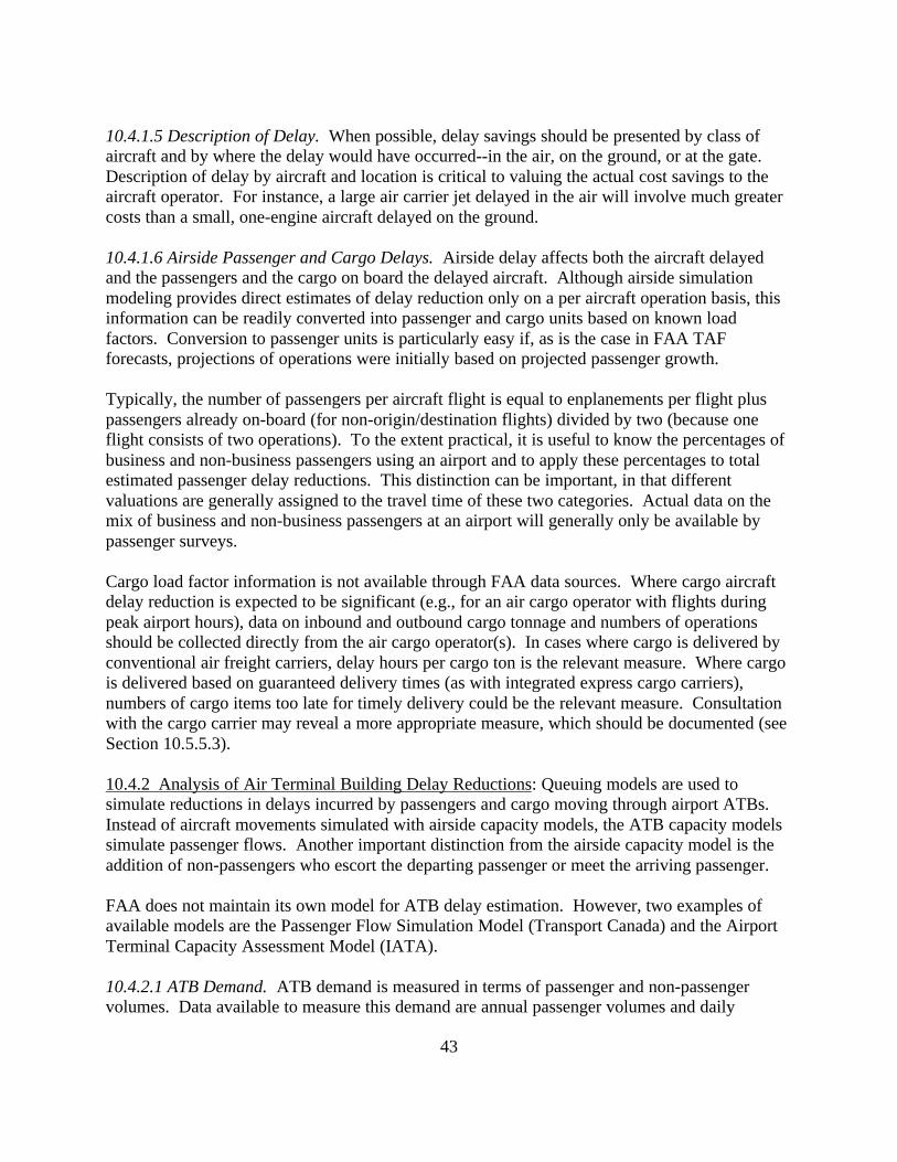
43

10.4.1.5 Description of Delay. When possible, delay savings should be presented by class ofaircraft and by where the delay would have occurred--in the air, on the ground, or at the gate.Description of delay by aircraft and location is critical to valuing the actual cost savings to theaircraft operator. For instance, a large air carrier jet delayed in the air will involve much greatercosts than a small, one-engine aircraft delayed on the ground.

10.4.1.6 Airside Passenger and Cargo Delays. Airside delay affects both the aircraft delayedand the passengers and the cargo on board the delayed aircraft. Although airside simulationmodeling provides direct estimates of delay reduction only on a per aircraft operation basis, thisinformation can be readily converted into passenger and cargo units based on known loadfactors. Conversion to passenger units is particularly easy if, as is the case in FAA TAFforecasts, projections of operations were initially based on projected passenger growth.

Typically, the number of passengers per aircraft flight is equal to enplanements per flight pluspassengers already on-board (for non-origin/destination flights) divided by two (because oneflight consists of two operations). To the extent practical, it is useful to know the percentages ofbusiness and non-business passengers using an airport and to apply these percentages to totalestimated passenger delay reductions. This distinction can be important, in that differentvaluations are generally assigned to the travel time of these two categories. Actual data on themix of business and non-business passengers at an airport will generally only be available bypassenger surveys.

Cargo load factor information is not available through FAA data sources. Where cargo aircraftdelay reduction is expected to be significant (e.g., for an air cargo operator with flights duringpeak airport hours), data on inbound and outbound cargo tonnage and numbers of operationsshould be collected directly from the air cargo operator(s). In cases where cargo is delivered byconventional air freight carriers, delay hours per cargo ton is the relevant measure. Where cargois delivered based on guaranteed delivery times (as with integrated express cargo carriers),numbers of cargo items too late for timely delivery could be the relevant measure. Consultationwith the cargo carrier may reveal a more appropriate measure, which should be documented (seeSection 10.5.5.3).

10.4.2 Analysis of Air Terminal Building Delay Reductions: Queuing models are used tosimulate reductions in delays incurred by passengers and cargo moving through airport ATBs.Instead of aircraft movements simulated with airside capacity models, the ATB capacity modelssimulate passenger flows. Another important distinction from the airside capacity model is theaddition of non-passengers who escort the departing passenger or meet the arriving passenger.

FAA does not maintain its own model for ATB delay estimation. However, two examples ofavailable models are the Passenger Flow Simulation Model (Transport Canada) and the AirportTerminal Capacity Assessment Model (IATA).

10.4.2.1 ATB Demand. ATB demand is measured in terms of passenger and non-passengervolumes. Data available to measure this demand are annual passenger volumes and daily

44

passenger volumes, augmented by a factor (determined through a survey specific to the airport)to reflect non-passengers who accompany passengers. As time savings benefits must becalculated at or close to peak operating conditions, data on passenger and non-passenger volumesby time of day must be assembled.

10.4.2.2 ATB Capacity. ATB capacity and the utilization or strain on that capacity are vitalcomponents to establishing proper investment impacts on time-in-ATB. However, determinationof capacity is the most difficult aspect of ATB evaluation. While it is relatively easy to measurethe processing capacity of each processor of passengers and the storage capacity of each ATBarea, the interaction of these components and their combined effect on capacity is difficult todetermine.

The needed variables for capacity determination are as follows: maximum practical capacity(MPC); peak system utilization index (PSI); hourly system utilization index (HSI); and mean-to-peak ratio (MPR). The capacity of the airport system as a whole--the MPC--is a function of thedemand pattern placed upon it. It is defined as the maximum number of passengers and non-passengers per hour that can be processed through the ATB without exceeding either the storagecapacity or the processing capacity of any subsystem. System utilization or congestion indicescan be calculated for ATBs using the MPC. Other indexes such as the PSI (the measure ofintensity of use during the planning peak), the HSI (the measure of utilization during all airportoperating hours), and the MPR (a measure of the severity of peaking) might also be of use.

Other indices of capacity relate to spatial and non-spatial ATB limitations. Spatial limitationsinclude the airport size (measured in total floor space or ATB user walking distance). Non-spatial capacity measures included the number of processing stations (including ticketing,baggage handling, and security). Measures include ATB active walking space and mean walkingdistance.

10.4.3 Quantification of Landside Delay Reduction: Automobile traffic simulation models areavailable through public and proprietary sources. However, the FAA has not extensively studiedthem. Once such model is the MicroBENCOST model,7 but other traffic models exist and areacceptable. Assistance should be sought through State and local planning boards and highwaydepartments, who will also have important inputs with regard to overall traffic planning for theairport environs. Simulation analysis must consider capacity and peak factors comparable tothose of ATB modeling, although the focus of the analysis should include vehicles as well aspassenger volumes.

10.4.4 Improved Schedule Predictability: Measurement of the time and resources allocated byaircraft operators specifically to accommodate potential airport delays is difficult. Delay

7See "MicroBENCOST Program Documentation" and "Microcomputer Evaluation ofHighway User Benefits: Final Report for NCHRP 7-12" prepared for the NationalCooperative Highway Research Program by the Texas Transportation Institute,Texas A&M University System, College Station, Texas 77843, October 31, 1993.

45

accommodation practices will vary by operator, airport and city, prevailing weather conditions,and time of day. Passengers will also adjust their schedules to different degrees to accommodatepotential delay at airside, ATB, and/or landside depending on their past experience with delay atthe airport, the time sensitivity of their trips, and other factors.

Surveys of aircraft operators, passengers, and freight companies are the best means to quantifythe amount of time allowed for potential delay. Operators and passengers should provideinformation on their delay accommodation behavior given present delay experience, and shouldbe asked to provide information on their anticipated delay accommodation behavior if thefrequency and/or severity of delays is altered. These responses can then be matched to theestimated delays associated with the base case and investment alternatives.

The estimated reduction in total hours of time and resources allotted for potential delays as aresult of an investment alternative must be reduced by the total estimated hours of actual delayreduction caused by that alternative to avoid double-counting. In other words, if a 2 minuteaverage delay reduction induces the passenger to reduce time allotted to potential delays by anaverage 3 minutes, the net saving per passenger attributable to schedule predictability is 1 minute(the other 2 minutes are already accounted for by the actual delay reduction). Time savingsattributable to schedule predictability should be attributed to the source of the improvedpredictability, either at airside, ATB, or landside.

10.4.5 More Efficient Traffic Flows: Benefits to aircraft operators and passengers associatedwith more efficient airside traffic flow derive from shorter travel distances (in vectoring andtaxiing) and the associated reduction in aircraft operating hours. These reductions are generallycaptured in the airfield modeling exercise used to measure delay, but are not, strictly speaking,delay benefits. This is because the same time savings will be realized regardless of congestionlevels. Time savings associated with improved aircraft traffic flows (as distinct from delayreductions associated with decreased congestion) should be quantified and presented separatelyin the BCA.

Benefits to passengers from shortened pedestrian traffic distances in redesigned ATBs can bemeasured in reduced passenger time required to transit these distances. These time reductionsmeasured in the ATB modeling exercise should be quantified and presented separately from timesavings associated with reduced ATB congestion, if possible. Alternatively, in the case of someATB expansions, walking distances may actually be lengthened. In such cases, the benefits ofreduced congestion will be offset to some extent by the longer walking times.

10.4.6 Use of Larger, Faster and/or More Efficient Aircraft: The ability of a new project toenable the use of larger, faster, and/or more efficient aircraft is a potentially important butdifficult-to-quantify capacity benefit. Whereas a new, long runway may permit an airport toaccommodate larger aircraft for flights to more distant locations (thus reducing circuitous routingthrough hubs and/or operating costs), actual use of this new capability at an airport by aircraftoperators is uncertain. Similarly, it is often difficult to anticipate how airlines may change theiraircraft mixes and route structures in response to greater flexibility.

46

The airport sponsor must obtain data to measure the following impacts of service by more larger,faster, and/or more efficient aircraft:

• The impact of new services and aircraft on the prevailing cost and fare structure at theairport; and

• The reduced transit time enabled by new routes and/or aircraft.

These data can be developed from one or more of the following methods:

• Analysis of air service at comparable airports with runways of similar length to theproposed extended runway;

• Interviews with air carriers and other air service concerning their interest in, plans for,and commitment to the extension; and

• Surveys of passengers concerning potential demand for expanded services.

Selection of a particular method will depend on several factors, including the complexity andcost of the project and difficulty in collecting data. Complex or costly projects may require allthree methods.

10.4.6.1 Interviews with Air Service Providers. Conferring with potential air service providers atthe study airport can yield important information. The air service providers may have well-developed business plans for new services they intend to provide from an expanded facility,developed using sophisticated route and network analysis models. Care should be taken toacquire from each operator any available documentation which supports its assessments of thepotential time or cost savings of the expansion (e.g., market surveys, cost savings attributable tomore efficient aircraft) of the project in question.

Particular care should be used in assessing the realism of planned business expansions. FAAwill heavily discount benefits claimed for projects that are not supported with documentationfrom current airport users. Similar scrutiny will be applied to benefit estimates for unspecifiedfuture operators or start-up operators who lack sufficient capitalization to support major activityexpansions. Finally, FAA will view with caution claims for future use by operators who havelittle financial exposure should their plans for the new facility prove too optimistic.

10.4.6.2 Passenger Surveys. In the case of large or expensive projects, it is advisable thatinterviews with aircraft operators be supplemented with surveys of passengers and freightshippers with access to the study airport. Surveys should seek to determine whether passengersand/or air freight shippers would be responsive to proposed new services at the study airportbased on expected routes, fares, schedules, and convenience of access to the study airport. Aircarriers and other users of the airport should be consulted on the outcome of these surveys tocheck for reasonableness.

47

10.4.6.3 Analysis of Air Service at Comparable Airports. This approach involves collecting dataon the actual types of services, fares, trip times, and other service measures at airportscomparable in size and situation to the study airport. Ideally, if comparison airports can be foundwhich vary from the study airport chiefly with regard to the facility being studied, benefits forthe proposed facility can be estimated from the difference in the service measures between thecomparison and study airports.

Comparability of airports should be established at several levels. Comparison airports should beselected based on:

• Comparable airport size and traffic levels to the study airport;• Similar airport infrastructure, both before and after the investment being studied; and• Location in communities with demographic (population, per capita income) and

economic (business and industry) bases similar to those of the study airport.

As many comparison airports as possible should be studied, with at least 5 identified andanalyzed. To the extent possible, airports should be from the same geographic region, in thatregional factors such as weather, labor costs, and service providers can cause significant cost andservice differences among regions. In addition, airports from the same region are more likely tohave comparable average trip lengths (which reflect distance from the airport to the finaldestination).

Analysis should focus on the different passenger enplanements, air routes, trip times, and farestructures between the comparison and study airports. Data of this type are available fromcommercial vendors of aviation data provided by air carriers to the Department of TransportationBureau of Transportation Statistics.8 To the extent possible, causes for differences in servicefactors other than facility constraints at the study airport should be identified and discussed. Themore comparison airports that are identified, the more confidence can be assigned to identifieddifferences.

Of particular interest to a benefits analysis are differences between the airports with regard tofares and average trip times. In a competitive service market, lower fares per passenger arelikely to reflect lower costs of providing air service at the airport. Lower costs may, in turn,reflect the use of more efficient aircraft. Average fares can be derived by multiplying averageyield per revenue passenger mile (RPM) by average trip length. Assuming travel patterns(destination cities) and other non-infrastructure factors (passenger volumes) do not varysignificantly among the comparison and study airports, systematically lower fares at thecomparison airports may indicate lower costs attributable to their possession of the facility inquestion. Similar inferences can be considered in the case of shorter overall trip times. Shortertrip times may be the result of faster aircraft (jets rather than turboprops) and more direct flights.

8Unfortunately, aircraft cost information is not available on an airport

specific basis.

48

A methodology for interpreting and valuing fare and trip time differences on a per passengerbasis is presented in the Section 10.5.8.

10.4.6.4 Other Methods. FAA is receptive to any additional methodology for measuring thepotential impact of infrastructure that accommodates larger, faster, or more efficient aircraft.Such methodology should be clearly described and documented.

10.4.7 Safety, Security, and Design Standard Benefits Associated With Capacity Projects: Asnoted in Section 10.3.4, FAA does not require a BCA for projects principally intended toaccomplish safety, security, or design standards objectives. However, there are safety, security,and design standard benefits associated with some capacity projects.

10.4.7.1 Compliance With Safety, Security, and Design Standards. No benefit can be claimed forthe compliance of a capacity project with FAA design standards (Section 10.3.1.5). However,some capacity projects may have a positive impact on standards compliance of pre-existingairport infrastructure. When this occurs, a standards benefit can be assigned to the capacityproject BCA equal to the cost-saving associated with the mitigation of the standards problemelsewhere on the airport.

The compliance credit cannot exceed the cost of the least-cost alternative means ofaccomplishing the remedial compliance objective that is also acceptable to FAA. In other words,if the capacity project eliminates the need to expand a runway safety area elsewhere at theairport, the credit allowed in the BCA would not necessarily be the cost of expanding the safetyarea. Instead, it might be the cost of implementing a declared distances policy or some otheroperating restriction that would accomplish the same safety objectives. The costs of physicalcorrections should be derived from engineering estimates. The impact of a safety-relatedoperating restriction on hours of delay at the airport can be measured using capacity simulationmodels.9

10.4.7.2 Increased Safety Associated with Precision Approaches. In instances where a potentialcapacity improvement will lead to an overall increase in the level of the precision approach to anairport (e.g., moving from only non-precision approaches to an ILS 1 system), FAA's Office ofAviation Policy and Plans will calculate the safety benefits attributable to this improvement. Indoing so, FAA will comply with the current precision landing systems establishment criteria.

9In many cases where an airport does not meet FAA standards an operatingrestriction will already be in place. Delay reductions attributable to theremoval of a pre-existing operating restriction will most likely already becaptured through the simulation analysis described in section 10.4.1 and shouldnot be double-counted. However, to the extent possible, this source ofbenefits should be separately categorized.

49

10.4.8 Environmental Benefits Associated With Capacity Projects: Projects undertakenprincipally to meet environmental objectives are not subject to FAA BCA requirements (seeSection 10.3.5). Moreover, no benefit can be claimed for the compliance of a capacity projectwith Federal environmental standards (see Section 10.3.1.7). However, most airport capacityprojects will have environmental impacts which should be included in the BCA as either benefits(positive environmental impacts) or costs (negative environmental impacts).

10.4.8.1 Noise Benefits. Measurement of noise impacts associated with capacity projects can beperformed using various models. The Integrated Noise Model (INM) (Version 4.11) is currentlyused by FAA and is required in most noise assessments prepared for FAA. INM and relatedmodels reveal the extent of aircraft noise impacts by mapping regions that are unacceptablyimpacted. As such, noise models indicate the number of residences or structures that must eitherbe purchased or modified to mitigate impacts under various scenarios.

INM analysis of a capacity project may reveal that a runway distributes noise away from animpacted area and thus reduces the number of homes (now or in the future) within the 65 and 70DNL zones. This reduction would eliminate the need to purchase or soundproof these homes.The analyst should be specific about the timing of this impact. For instance, relative to the basecase, the 65 DNL zone might be reduced by 250 homes in year X and 500 homes in year X+5.In this case, a benefit of 250 homes would be cited in year X and 250 homes in year X+5 (theincrement in homes from year X to year X+5).

10.4.8.2 Air Emissions. The Emissions and Dispersion Modeling System (EDMS) enablesanalysts to calculate the air quality at airports caused by all pollution sources (e.g., aircraft andpassenger and employee automobiles). EDMS and other models will indicate the amounts ofpollutants emitted by various airport sources under different operating scenarios. The FAAOffice of Environment and Energy (AEE) should be consulted on the potential use of this model.

10.4.9 Lower Airport Operations and Maintenance (O&M) Costs: Airport investments willfrequently lead to reductions in the resources needed to operate and maintain the airport, thusproviding greater efficiency and productivity. For example, rebuilding of an ATB toaccommodate additional passengers will also provide cost savings in the form of lower resourcesneeded to operate and maintain the new structure. Efficiency savings may involve reductions inthe number of airport personnel required to serve each passenger, reduced electrical powerrequirements, and other reductions in utility requirements. Although these savings are oftentreated as benefits (i.e., foregone costs), FAA categorizes O&M as a life-cycle cost item. Assuch, FAA recommends that O&M savings associated with different investment alternatives besummarized in the project cost component of the BCA.

10.5 Step 3--Valuation of Benefits: The methods described in Section 10.4 will yieldestimates of the actual units of resources saved or generated by alternative investments relative tothe base case. In order to aggregate these benefits into one overall monetary measure sothat they can be compared to costs, economic values must be attached to each measured resourceunit. Prior to discussing the valuation of individual benefit units developed in Section 10.4, it is

50

appropriate to describe some of the general economic concepts that underlie the valuation ofresource units, including the use of constant dollars and the treatment of incremental andfractional units.

10.5.1 Constant Dollars: All economic values for benefits and costs should be assigned in termsof constant (real) dollars of given year--usually the year in which the BCA is conducted. If theBCA study takes place in 1999, the value of a unit of output from a project (regardless of thefuture year in which it is realized) should be presented in terms of its 1999 dollar value.

A unit of a given output will generally maintain the same constant dollar value throughout aproject's life. Only in a situation where the relative value of an output is expected to change overtime (i.e., a unit of this output will become relatively more valuable when valued in terms ofother real outputs) would application of a changing value (in constant dollars) be appropriate.The use of constant dollars greatly reduces the complexity of later discounting of benefits andcosts.

10.5.2 Equal Valuation of Incremental Units: FAA recommends that incremental benefit unitsof the same type be valued equivalently to each other. That is, the hundredth unit of benefit Xshould be assigned an economic value equivalent to the thousandth unit of benefit X. For certainprojects generating very large benefit flows, this practice may lead to an incorrect valuation ofincremental benefits (due to the economic concept of diminishing marginal utility). However,the difficulty and uncertainty associated with accurate measurement of marginal changes in unitvalue will generally exceed the potential addition to accuracy associated with adjusting values.

10.5.3 Valuation of Fractional Benefit Units: Aggregate measurements of benefits are oftencomposed of large numbers of fractional unit savings. For instance, a total annual time savingassociated with a project may be 2,000 hours, but this total may be assembled from manythousands of individual times savings ranging from 1 minute to half an hour or more. It isDepartment of Transportation policy that fractional benefit units be valued at the same per unitvalue as whole units. In other words, if an hour of passenger time is worth $X, a saving of 5minutes of passenger time should be valued at 1/12 $X. This recommendation is economicallyjustified and greatly simplifies the valuation of total project benefits.

Some economists argue that small, fractional-hour time savings should be valued at a lower perunit rate than longer time savings (e.g., an hour per person) because they are too small to be usedeffectively or to be noticed by the traveler. FAA has contended that all time savings, fractionalor otherwise, be valued at the same per hour rate for following reasons:

• The generally accepted theory of the value of time savings does not distinguish betweenfractional units of time and larger amounts;

• There is no evidence that travelers value small time saving at a different rate than largertime savings;

• Average time savings generated by simulation models may mask wide variations inindividual delay experiences. For instance, an investment may save 3 persons out of 60

51

one hour of delay each, whereas the other 57 persons may experience no saving. Theaverage delay saving per passenger would be 3 minutes--an amount that may appear to betoo small to be useful even though it is actually realized in larger units;

• The definition of a particular "threshold" (e.g., 10 minutes) for useful time savings wouldbe arbitrary;

• Time savings are cumulative over the length of an entire trip. For instance, if a personincurs nine minutes of delay savings from non-airport sources (either aviation or non-aviation), a one minute additional delay saving at the study airport would push thisperson over a 10 minute "threshold" (were such a threshold valid); and

• Similarly, suppose several separate projects are under consideration at an airport and eachwould save the same traveler one to 3 minutes. If the small time savings were valued at alower rate or not at all, it is likely that none of the projects would pass a BCA. However,if considered collectively, the projects' benefits could exceed a particular threshold andreceive full value. Under this scenario, the projects may be shown to be cost-beneficial.

10.5.4 Summary of Unit Values for Benefits: Table 10.4 summarizes the unit values that shouldbe applied to each of the benefit types quantified in Section 10.4.

10.5.5 Valuation of Delay Reductions: Once the number of hours of delay reduction for aircraft,passengers, cargo, and (if quantified) passenger meeter/greeters has been determined, a per hourvalue should be assigned. The following information expands on Table 10.4.

10.5.5.1 Valuation of Aircraft Delay Reductions. Estimated annual hours of reduced delayshould be multiplied by appropriate per hour variable operating costs to yield annual estimates ofthe value of saved aircraft delay. The value of an hour of reduced aircraft delay is usually

52

TABLE 10.4: VALUATION OF AIRPORT PROJECT BENEFITSBENEFIT UNIT VALUATION SOURCE OF VALUE DATAReduced Aircraft Delay Hours• Reduced aircraft delay

hours by airborne, taxi, orgate status for eachaircraft class (air carrier,commuter, GA, military)

Operating cost per aircrafthour, adjusted for aircraftclass and delay locationstatus. In limited cases,saved aircraft capital costmay be considered.

Documented operating costdata (net of depreciation)provided by aircraft operators(if available). Consult FAA-APO-98-8for aircraft type orclass values by block hour.Where aircraft fleet size canbe reduced due to large delaysavings, use published usedaircraft values (see FAA-APO-98-8). FAA-APO-98-8 alsocontains current lease values.

Reduced Passenger Delay Hours• Reduced business and

non-business passengerdelay hours by airside,ATB, and landside status

Passenger willingness to payto avoid one hour of traveldelay

FAA-APO-98-8 contains thepassenger travel time valueswhich OST has developed andrequires FAA to use.

• Reduced passengervehicle hours in landsideaccess

Passenger vehicle operatingcosts

Current FHWA estimates.

Reduced Air Cargo Delay Hours• Reduced air cargo ton

hours by airside, ATB, andlandside status

Opportunity cost of cargodelayed in transit/Spoilage oftime sensitive cargo

Documented data on value ofcargo provided by operators(if available). Apply 7 percentreal opportunity cost (annualbasis) to value of cargo forperiod delayed.

• Units of express cargoarriving late at airportafter time required tomake guaranteed deliverytime

Refunded shipping revenuefor late package delivery orgreater resource costsexpended to compensate forairport delays

Documented data provided byoperators.

• Reduced trucking hours inlandside access

Cargo vehicle operating costs Current FHWA estimates forlight trucks (including drivercosts).

Reduced Meeter/Greeter Delay Hours• Reduced meeter/greeter

delay hours by airside,ATB, and landside status

Meeter/greeter willingness topay to avoid one hour ofdelay

FAA has not assigned a valueto meeter/greeter time.Sensitivity analysis shouldassume half the values appliedto passenger time in FAA-APO-98-8.

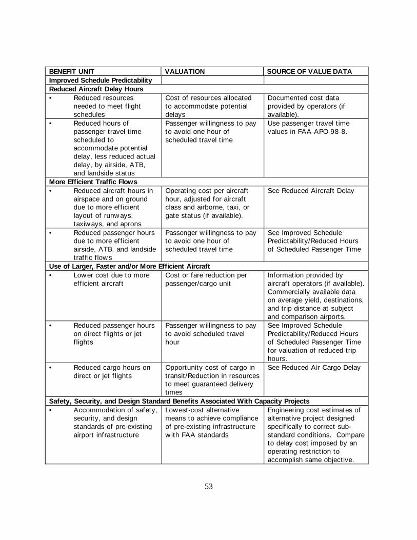
53

BENEFIT UNIT VALUATION SOURCE OF VALUE DATAImproved Schedule PredictabilityReduced Aircraft Delay Hours• Reduced resources

needed to meet flightschedules

Cost of resources allocatedto accommodate potentialdelays

Documented cost dataprovided by operators (ifavailable).

• Reduced hours ofpassenger travel timescheduled toaccommodate potentialdelay, less reduced actualdelay, by airside, ATB,and landside status

Passenger willingness to payto avoid one hour ofscheduled travel time

Use passenger travel timevalues in FAA-APO-98-8.

More Efficient Traffic Flows• Reduced aircraft hours in

airspace and on grounddue to more efficientlayout of runways,taxiways, and aprons

Operating cost per aircrafthour, adjusted for aircraftclass and airborne, taxi, orgate status (if available).

See Reduced Aircraft Delay

• Reduced passenger hoursdue to more efficientairside, ATB, and landsidetraffic flows

Passenger willingness to payto avoid one hour ofscheduled travel time

See Improved SchedulePredictability/Reduced Hoursof Scheduled Passenger Time

Use of Larger, Faster and/or More Efficient Aircraft• Lower cost due to more

efficient aircraftCost or fare reduction perpassenger/cargo unit

Information provided byaircraft operators (if available).Commercially available dataon average yield, destinations,and trip distance at subjectand comparison airports.

• Reduced passenger hourson direct flights or jetflights

Passenger willingness to payto avoid scheduled travelhour

See Improved SchedulePredictability/Reduced Hoursof Scheduled Passenger Timefor valuation of reduced triphours.

• Reduced cargo hours ondirect or jet flights

Opportunity cost of cargo intransit/Reduction in resourcesto meet guaranteed deliverytimes

See Reduced Air Cargo Delay

Safety, Security, and Design Standard Benefits Associated With Capacity Projects• Accommodation of safety,

security, and designstandards of pre-existingairport infrastructure

Lowest-cost alternativemeans to achieve complianceof pre-existing infrastructurewith FAA standards

Engineering cost estimates ofalternative project designedspecifically to correct sub-standard conditions. Compareto delay cost imposed by anoperating restriction toaccomplish same objective.

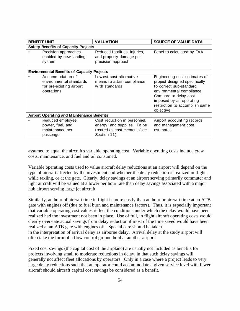
54

BENEFIT UNIT VALUATION SOURCE OF VALUE DATASafety Benefits of Capacity Projects• Precision approaches

enabled by new landingsystem

Reduced fatalities, injuries,and property damage perprecision approach

Benefits calculated by FAA.

Environmental Benefits of Capacity Projects• Accommodation of

environmental standardsfor pre-existing airportoperations

Lowest-cost alternativemeans to attain compliancewith standards

Engineering cost estimates ofproject designed specificallyto correct sub-standardenvironmental compliance.Compare to delay costimposed by an operatingrestriction to accomplish sameobjective.

Airport Operating and Maintenance Benefits• Reduced employee,

power, fuel, andmaintenance perpassenger

Cost reduction in personnel,energy, and supplies. To betreated as cost element (seeSection 11).

Airport accounting recordsand management costestimates.

assumed to equal the aircraft's variable operating cost. Variable operating costs include crewcosts, maintenance, and fuel and oil consumed.

Variable operating costs used to value aircraft delay reductions at an airport will depend on thetype of aircraft affected by the investment and whether the delay reduction is realized in flight,while taxiing, or at the gate. Clearly, delay savings at an airport serving primarily commuter andlight aircraft will be valued at a lower per hour rate than delay savings associated with a majorhub airport serving large jet aircraft.

Similarly, an hour of aircraft time in flight is more costly than an hour or aircraft time at an ATBgate with engines off (due to fuel burn and maintenance factors). Thus, it is especially importantthat variable operating cost values reflect the conditions under which the delay would have beenrealized had the investment not been in place. Use of full, in flight aircraft operating costs wouldclearly overstate actual savings from delay reduction if most of the time saved would have beenrealized at an ATB gate with engines off. Special care should be takenin the interpretation of arrival delay as airborne delay. Arrival delay at the study airport willoften take the form of a flow control ground hold at another airport.

Fixed cost savings (the capital cost of the airplane) are usually not included as benefits forprojects involving small to moderate reductions in delay, in that such delay savings willgenerally not affect fleet allocations by operators. Only in a case where a project leads to verylarge delay reductions such that an operator could accommodate a given service level with feweraircraft should aircraft capital cost savings be considered as a benefit.

55

At airports served by a relatively small number of air carriers, variable operating cost data can becollected directly from the aircraft operators. However, at many airports, comprehensive surveysof aircraft operators may be impractical due to the reluctance of some to share data or simply dueto the large numbers of operators (particularly where GA is a major component of traffic).

A comprehensive discussion of aircraft operating cost and other economic values relevant toairport project BCAs is available in the FAA publication "Economic Values for Evaluation ofFederal Aviation Administration Investment and Regulatory Programs" (FAA-APO-98-8,June 1999). This publication specifically addresses aircraft operating costs (for both air carrierand GA) and also covers aircraft capital costs (in the form of aircraft replacement costs). Inaddition to describing data sources, the publication presents tables of values for different aircrafttypes. Values should be converted to current dollars using the methodology described foraircraft variable operating costs in FAA-APO-98-8 (also see Appendix A of this guide for moreinformation on use of price indexes).

10.5.5.2 Valuation of Passenger Delay Reductions. Reductions in delay hours to passengers arevalued according to the willingness of passengers to pay to avoid travel delay.

The value used in the BCA should that described in FAA-APO-98-8. If the mix of business andnon-business passengers is known, the separate value estimates for these categories can beapplied to the pro-rated portions of the delay reduction reflecting these two passenger groups.

In the case of landside project where delay reductions lead to decreased use of passengervehicles, a value equal to the reduced variable operating costs of the vehicles may be attributedto reduced vehicle hours. The Federal Highway Administration should be consulted for data onautomobile variable operating costs.

10.5.5.3 Valuation of Air Cargo Delay Reductions. Whereas Section 10.4.1.6 propose a basicmeans for quantifying cargo delay in terms of hours, FAA has not settled on a generalmethodology for valuing reductions in shipping time for air cargo. Thus, the following guidanceon valuation is intended only to suggest possible approaches that would be acceptable to FAA.FAA encourages the development of innovative alternative approaches, provided they are well-documented and reproducible.

Conventional Air Cargoes. In most cases, the cost of delay in the delivery ofconventional air cargo (belly cargo and cargo carried by traditional all-cargo carriers) will beabsorbed by the shipper and/or recipient of the air cargo. Delay to shippers and/or recipients indelivery of non-perishable cargo can be conservatively valued based on the average value of aton of air cargo multiplied by OMB's estimate of the return to capital in the U.S. economy.10 Byway of example, if a ton of cargo valued at $5 million is delayed by 2 hours, the cost of thisdelay would equal $5 million multiplied by 2, divided by 8760 hours (the hours in one year), and 10See Section 12 for a discussion of the time value of money.

56

then multiplied by 7 percent (yielding $80). In the case of perishable cargoes, such as freshproduce or flowers, the cost of spoilage or reduced shelf life should be estimated, documented,and added to the estimated time value of an hour of delay.

Delay may also result in critical logistical problems for shippers, leading to large expenses orrevenue losses. Unfortunately, estimation of these costs is highly situation-specific andextremely difficult to document.

Guaranteed Delivery Cargoes. Delays incurred by integrated, door-to-door packagecarriers can result in direct monetary losses to the carrier, either due to refunded shipping fees orhigher operating costs needed to expedite late packages. If clearly documented, these highercosts per package delay hour could be used to measure the value of measured delay savings. Asin the case of conventional air cargo, the package recipient may have important logistical needsfor package. In many cases, the refund of the shipping fee will not compensate these parties forthe late delivery of a critical package or part. Unfortunately, there is no method to capture fullythis impact, which will vary widely based on circumstance.

Required Documentation. Both in the case of conventional and integrated cargoes, it isclear that the high degree of reliance on data provided by proprietary operators places a premiumon documentation of claimed benefits by the operators in question.

10.5.5.4 Valuation of Meeter/Greeter Delay Reductions. FAA has not yet established a formalpolicy recognizing the role of benefits to persons who meet or escort people at ATBs, nor has itdeveloped formal values to be applied to reductions in meeter/greeter delay time. Meeter/greeteractivity is often voluntary and not essential to completion of the air trip. On the other hand, themeeter/greeter's time clearly has a real value to both the meeter/greeter and, presumably, to thepassenger accompanied. Until FAA is able to establish a firm value per hour of meeter/greeterdelay, it is recommended that meeter/greeter time be valued at one-half of the value assigned tothe passenger associated with the meeter/greeter. Moreover, it is recommended that themeasured benefit should not be included as a core benefit in the BCA, but rather should betreated as qualitative information to the BCA.

10.5.6 Improved Schedule Predictability: Valuation of reduced time allotted for potential delays(whether incurred airside, landside, or in the ATB) is done by multiplying the reduction in timeallocated for delays (less the reduction in actual delays) by the appropriate opportunity cost ofthat time. Aircraft, passenger, and cargo schedule time savings should be valued at the per hourrates defined in Section 10.5.5.11

11Time allocated to accommodate potential delays, as well as time spent innon-delayed travel, may be valued at a somewhat lower rate than time spent inunexpected delay. Consequently, Table 10.4 is structured to allow thepotential placement of different time values for scheduled travel time asopposed to unscheduled time. FAA official values for time should be usedpending further notification.

57

10.5.7 More Efficient Traffic Flows: Estimated reductions in travel time attributable to moreefficient airside, ATB, and landside infrastructure are frequently mixed in with estimatedreductions in delay as determined by capacity models. However, when possible, benefitsassociated with more efficient design should be isolated and valued separately according to thesame values defined for delay in Section 10.5.5.

10.5.8 Use of Larger, Faster, and/or More Efficient Aircraft: Benefits associated with airsideimprovements that enable larger, faster, and/or more efficient aircraft to serve an airport aremeasured both in the form of reduced cost per revenue passenger mile and reduced passengertime in transit.

10.5.8.1 Lower Cost Per Revenue Mile. Information provided by carriers on cost reductionsassociated with the use of more efficient aircraft may be used directly if the information is welldocumented.

10.5.8.2 Reduced Time In Transit. Trip time reductions due to faster aircraft and/or more directflights can either be derived from carrier-provided information or by study of trip times atcomparison airports. Reduced time in transit should be valued at the standard value per hour ofpassenger time or cargo time (see Section 10.5.5).

10.5.9 Safety, Security, and Design Standard Benefits Associated With Capacity Projects: Thestandards compliance credit that can be taken for a capacity project that corrects a pre-existingstandards problem at an airport cannot exceed the most cost-effective alternative means to havecorrected the problem. Determination of this value will equal the lesser of the lowest costphysical correction (determined through engineering estimates) or the lowest cost operationsrestriction (estimated by simulation modeling of delays and other inefficiencies imposed by therestriction). Aircraft, passenger, and cargo delays associated with operating restrictions wouldbe valued using the methodologies described in section 10.5.5.

10.5.10 Safety Benefits of Capacity Projects: FAA will assign appropriate values to safetybenefits associated with upgrades in precision landing systems. Guidance on appropriate valuesto assign to avoided fatalities, injuries, and property damage are provided in FAA-APO-98-8.Values for avoided fatalities and injuries, when updated by the Office of the Secretary ofTransportation, are published in FAA/APO bulletins.

10.5.11 Environmental Benefits of Capacity Projects: The environmental credit that can be takenfor a capacity project that mitigates a pre-existing environmental problem at an airport cannotexceed the most cost-effective alternative means to have corrected the problem. Determinationof this value will equal the lesser of the lowest cost physical correction (determined throughengineering estimates) or the lowest cost operations restriction (estimated by simulationmodeling of delays and other inefficiencies imposed by the restriction). Aircraft, passenger, andcargo delays associated with operating restrictions would be valued using the methodologiesdescribed in section 10.5.5.

58

10.5.12 Airport Operating and Maintenance Benefits: Reductions in the resources needed tooperate and maintain the airport (relative to the base case) should be treated in the cost side ofthe BCA. The analyst should consult airport accounting records and management cost estimatesto value these savings.

10.6 Hard-To-Quantify Benefit and Impact Categories: A natural follow-on to valuation ofthe benefits described in Section 10.3 is the identification and description of benefits and impactswhich are too difficult to quantify or cannot be evaluated in dollar terms--referred to in thisguidance as "hard-to-quantify" benefits and impacts. Hard-to-quantify benefits and impactsshould not be neglected and can be very important to the outcome of the analysis and a decisionon whether to pursue a particular alternative.

Hard-to-quantify benefits described below include:

• Measurement of systemwide delay caused by local airport delay;• Passenger comfort and convenience; and• Non-aviation macroeconomic and productivity impacts.

10.6.1 Systemwide Delay: Simulation modeling of delay at the study airport does not capturethe effect of "follow-on" delays, e.g., delays that result at other airports as a result of delaysoriginating due to congestion at the subject airport. Whereas FAA attempts to considersystemwide delay impacts in its capacity analyses, it has been unable to develop a robustsimulation methodology for measuring these impacts.

Efforts by FAA to simulate follow-on delay have emphasized the use of systemwide delaymodels such as the National Airspace System Performance Analysis Capability (NASPAC)model and the Airport Network Model (AIRNET). These tools permit the analyst to study thepotential effects of system performance problems, usually measured in terms of delays, as theypropagate through the nation over the course of a day. However, in practice, the models haveproved more useful for general diagnostic analysis (e.g., indicating which destination airports aremost sensitive to schedule disruptions) than in quantifying follow-on delay impacts. Problemswith the models include their inability to recreate the dynamic rescheduling undertaken byairlines in the event of major schedule disruptions or permanent changes in airport capacity.

Consideration of follow-on delay impacts is probably unwarranted for projects with fairly smallreductions in average delay (e.g., 2 minutes or less). However, in the case of projects with majoraverage delay reductions (5 minutes or more), the analyst may attempt to quantify follow-oneffects. FAA will consider follow-on delay reduction estimates developed from anymethodology that is well documented.

59

An example of a potentially usable methodology is one developed by Lincoln Laboratory.12 TheLincoln Laboratory approach is based on a matrix of probabilities that delays of various lengths(less than 10 minutes, 11 to 20 minutes, etc.) at one airport will carry over to downstreamairports. The analyst could retrieve data on flight delay reductions by flight from simulationmodel results and apply the specified probabilities from the Lincoln Laboratory matrix as a firstapproximation of total delay saved. Technical Supplement No. 3 of "A Study of the HighDensity Rule" (July 1995) illustrates one application of this methodology.

10.6.2 Increased Passenger Comfort and Convenience: Some capacity investments made atairports, particularly in ATB facilities, have the specific goal of improving the comfort andconvenience of passengers and persons accompanying them. Such improvements may have asignificant impact on the passenger's perception of the utility of flying from a particular airportand may yield benefits to both the airport and the airlines through increased enplanements andconcession revenues. Unfortunately, comfort and convenience are highly subjective benefits thatare difficult to quantify, particularly with regard to the utility of aesthetic considerations.

One gross measure of passenger comfort is the increase in square feet of non-concession publicareas. Other parameters that may be measured are seats available in waiting areas, number ofrest facilities, etc. Expanded concession areas also may be viewed as enhancing public comfort,but are not eligible for AIP grants and should not be included in project BCAs submitted to FAAfor consideration for AIP grants.

FAA does not have official economic values for measures of passenger comfort andconvenience. Consequently, presentation of data on improved passenger comfort (e.g., increasedsquare footage of public areas) will in most cases be supplemental to the BCA calculation.However, for projects where a major benefit is expected from improved passenger comfort, itmay be appropriate to undertake a contingent valuation study based on a survey of passengers.

A contingent valuation study involves constructing a survey methodology that asks people whatdollar amounts they would be willing to pay for improved comfort. The main disadvantage ofthis approach is that there is no assurance that the analyst will obtain reliable answers to surveyquestions since, unlike market decisions, individuals may have less of an incentive to give anhonest and thoughtful response to a survey question. Moreover, respondents may not accuratelyprocess amenity information presented to them. Special care must be taken in the contingentvaluation study to present benefits in a manner understandable to the passenger. Despite theselimitations, the contingent valuation survey methodology has potentially great usefulness,particularly in contexts in which good market data are not available.

12Boswell, Steve, Lincoln Laboratory, Massachusetts Institute of Technology:"Analysis of Downstream Impacts of Air Traffic Delay and Estimation ofDownstream Delay Reduction Due to ITWS," (August 1994, unpublished).

60

10.6.3 Non-Aviation Impacts: FAA is charged with making investments that improve the airportand airway system--investments that are funded by taxes on aviation users. As noted in Section2 of this guidance, non-aviation impacts to communities from airport investments are generallynot included in FAA BCA studies. In addition, Section 6(b)(3) of OMB Circular A-94 generallyrules out consideration in BCAs of employment or output multipliers that purport to measure thesecondary effects of government expenditures in measured social benefits and costs. On theother hand, OMB believes that true non-aviation benefits which result from investments inaviation infrastructure should be counted. An example might be preservation of wetlands as aresult of airport landbanking.

However, the FAA is receptive to information on certain classes of non-aviation impacts,including macroeconomic and productivity gains. Macroeconomic gains include the expansionof employment and income as a result of the investment project. Productivity gains includebenefits such as the restructuring of business logistics systems to take advantage ofimprovements in air service. Macroeconomic and productivity gains should be listed separatelyfrom the aviation user benefits estimated for the project and should not be included in BCAmeasures.

10.6.3.1 Macroeconomic Gains. Methodologies for estimating direct employment creation (viasurvey or input-output analysis) and indirect and induced employment multipliers (from input-output analysis) are well established. However, macroeconomic gains can only be treated as aform of benefit if they are "incremental." That is, they are gains only if they would not haveaccrued to the national economy in the absence of the project.

Applications of input-output methodologies often fail to measure incremental impacts properly.The relocation of an operation from one region to another (e.g., the relocation of an air cargohub) will generate apparent macroeconomic gains for the recipient region but will cost the donorregion comparable gains. Measurement and comparison of the macroeconomic impacts for eachregion (or at a national level) could well yield a neutral macroeconomic impact.

Similarly, the incrementality of direct, indirect, and induced multiplier effects hinges upon theextent of structurally unemployed labor and surplus productive capacity in the regional economy.A key element in evaluating incremental impacts involves comparing the direct employmentexpected to be generated by a project to the number of unemployed in the city or greatermetropolitan area where the investment is being undertaken. Only if (1) the expected number ofunemployed persons in the regional economy in a particular year is greater than or equal to thedirect, indirect, and induced employment impact in the same year and (2) the jobs are notdisplaced from another region, can the complete set of direct, indirect, and induced impacts beassumed to be fully realized. In the case when the estimated employment impact exceeds theexpected number of unemployed, the direct, indirect, and induced impacts are limited to thenumber of job vacancies in the local economy.

61

Presentation of macroeconomic gains should be accompanied with a detailed description of themethodology used to calculate these gains. However, even with the precautions recommendedabove, macroeconomic gains estimates will still be subject to large uncertainties because thestimulative macroeconomic effects of airport projects are generally small in relation to theoverall volume of national and regional macroeconomic activity.

10.6.3.2 Productivity Gains. Companies and workers may obtain productivity gains if theyrestructure their logistics of doing business due to improved airport facilities. These improvedlogistics are not measured in input-output models since these models almost always reflect afixed logistics technology.

Only a limited number of studies to date have attempted to quantify productivity gains.13 Inthese studies, data collected from a survey of industry are used to estimate elasticities (measuresof sensitivity) of gains to industry from changes in transportation system attributes. Based onthese estimates, schedules of gains corresponding to different levels of transportation systemimprovements can be derived.

As would be expected, potential gains from the logistics response by industry is contingent uponspecific firm and industry characteristics. Firms for which logistics costs are a large share oftotal cost and which operate on low margins are most likely to take advantage of the ability toimprove their logistics systems.

Relatively few airport projects will be candidates for productivity analysis, in that the projectmust result in a fundamental change in the cost of doing business. Such projects may includenew airports, major airport or access road expansions, or installation of runways that permitlarger aircraft to use the airport. Given the early stage of development of this type of analysis,FAA will consider claimed productivity gains separately from conventional BCA results.

10.7 Special Case of New Airports: One of the most difficult applications of BCA criteria isto new/replacement airports. Proposals for new airports could include the following:

• Construction of a regional airport to consolidate traffic from several smaller airports andthus realize more service and/or lower fares;

• Construction of an airport to replace an obsolete or poorly-situated airport that is subjectto severe delays or service limitations; and

• Construction of an airport to supplement a nearby congested airport.

13One such study is by Hickling Lewis Brod Inc., Measuring the RelationshipBetween Freight Transportation and Industry Productivity, TransportationResearch Board, National Research Council, 1995.

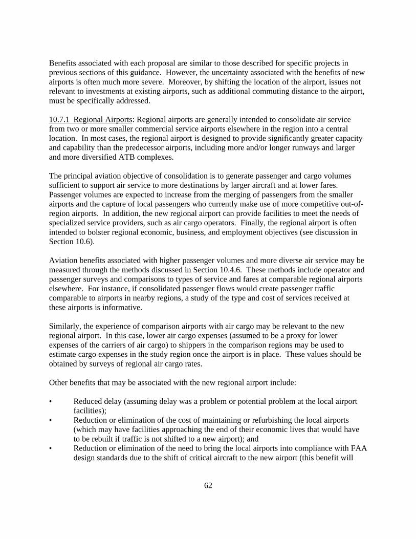
62

Benefits associated with each proposal are similar to those described for specific projects inprevious sections of this guidance. However, the uncertainty associated with the benefits of newairports is often much more severe. Moreover, by shifting the location of the airport, issues notrelevant to investments at existing airports, such as additional commuting distance to the airport,must be specifically addressed.

10.7.1 Regional Airports: Regional airports are generally intended to consolidate air servicefrom two or more smaller commercial service airports elsewhere in the region into a centrallocation. In most cases, the regional airport is designed to provide significantly greater capacityand capability than the predecessor airports, including more and/or longer runways and largerand more diversified ATB complexes.

The principal aviation objective of consolidation is to generate passenger and cargo volumessufficient to support air service to more destinations by larger aircraft and at lower fares.Passenger volumes are expected to increase from the merging of passengers from the smallerairports and the capture of local passengers who currently make use of more competitive out-of-region airports. In addition, the new regional airport can provide facilities to meet the needs ofspecialized service providers, such as air cargo operators. Finally, the regional airport is oftenintended to bolster regional economic, business, and employment objectives (see discussion inSection 10.6).

Aviation benefits associated with higher passenger volumes and more diverse air service may bemeasured through the methods discussed in Section 10.4.6. These methods include operator andpassenger surveys and comparisons to types of service and fares at comparable regional airportselsewhere. For instance, if consolidated passenger flows would create passenger trafficcomparable to airports in nearby regions, a study of the type and cost of services received atthese airports is informative.

Similarly, the experience of comparison airports with air cargo may be relevant to the newregional airport. In this case, lower air cargo expenses (assumed to be a proxy for lowerexpenses of the carriers of air cargo) to shippers in the comparison regions may be used toestimate cargo expenses in the study region once the airport is in place. These values should beobtained by surveys of regional air cargo rates.

Other benefits that may be associated with the new regional airport include:

• Reduced delay (assuming delay was a problem or potential problem at the local airportfacilities);

• Reduction or elimination of the cost of maintaining or refurbishing the local airports(which may have facilities approaching the end of their economic lives that would haveto be rebuilt if traffic is not shifted to a new airport); and

• Reduction or elimination of the need to bring the local airports into compliance with FAAdesign standards due to the shift of critical aircraft to the new airport (this benefit will

63

vary depending on the aviation role of the local facilities after the start-up of the regionalairport).

10.7.2 Replacement Airports: A replacement airport may be viewed as a special case of aregional airport. However, rather than consolidating traffic into one facility, its primary purposeis to replace a former central facility which has reached its maximum physical potential and/or issubject to some other permanent capacity constraint inherent to its location.

In general, the principal benefit associated with a replacement airport will be a reduction in delayassociated with alleviation of the capacity constraint at the former airport. However, benefitsmay also result from the accommodation of larger, faster, and/or more efficient aircraft whichcould not physically be accommodated at the predecessor airport. Other benefits describedabove for regional airports may also apply.

10.7.3 Supplemental Airports: Supplemental airports are those intended to accommodateregional demand that cannot be met by the existing, primary airport. Most typically, theseairports are termed reliever airports and are designed to accommodate general aviation trafficthat would otherwise use congested primary airports. However, in some cases, supplementalairports may take the form of full-fledged commercial service airports designed to accommodateall traffic types.

Benefits associated with supplemental airports are usually airspace and taxiway delay reductionsoccurring to users of both the reliever and the primary airport. These benefits can be modeledusing SIMMOD or other simulation models that can account for multi-airport airspacemanagement.

An important potential consideration is accessibility of the supplemental airport. Reallocation oftraffic to the airport on a voluntary basis may not occur if the reliever facility is too far removedfrom population or business centers of interest to its potential users. The issue of access and howit factors into BCA of new airports is discussed immediately below.

10.7.4 Uncertainties of Traffic Forecasts at New Airports: Extreme care must be used inassessing potential benefits attributed to higher traffic levels at new airports. In particular,passenger and cargo use of the airport may fall below expectations for the following reasons:

• Continued operation of the local airports the airport is intended to replace;• Lack of carrier interest in the new airport due to high user fees;• Poor location of the new airport relative to regional population centers; and• Proximity of a major hub airport within reasonable driving distance (e.g., 90 minutes) of

the new airport.

If smaller, local airports continue to operate after the opening of the new regional airport and arenot subject to major operating disadvantages, it is likely that some air service will continue to beprovided from the local airports. The degree to which this service will erode the level of traffic

64

at the new regional airport depends on locations relative to population centers, comparativelanding fee levels, and inducements offered to air service providers by local communities. Theuncertainty of traffic flows due to these factors should be assessed using surveys of potentialcarriers and passengers. For obvious reasons, lack of carrier support for the new airport must begiven major weight in situations where existing airports will remain open.

Landing fees associated with the pre-existing airports will generally be substantially less (for agiven level of traffic) than they would be for the new regional airport. This discrepancy resultsbecause the pre-existing airports have, in most cases, been fully amortized whereas the newairport will have significant bond payments to meet, even with AIP participation. Higher airportfees may mitigate variable operating cost savings that would result from the use of more efficientaircraft at the new airport (see Appendix C for more discussion on the effects of airport fees onpassenger travel decisions).

Location of the new airport at distances far away (20 miles or more) from regional populationcenters is another basis for concern about future traffic volumes. Ground access time is a majorconsideration of passengers who make trip decisions based on total transit time and air fare. Inparticular, benefits of estimated lower air fares and air transit times to passengers can be partiallyor completely eliminated by higher ground access times and expenses. Moreover, the lowerfares and air transit times that are the assumed inducement for passengers to use the new airportwill not be realized in the first place if sufficient passengers volumes are not attained at the newfacility. In this latter case, air service to the region could actually end up more fragmented andexpensive than it was before (especially if the pre-existing airports continue to operate).

Proximity of a major hub airport to the region (particularly an airport served by a discount aircarrier) introduces yet another element of uncertainty with regard to the recapture of lost regionaltraffic. Major fare savings may be associated with travel to the out-of-region airport whichcannot be matched at the new airport. In addition, if the air service from the more distant airportis more direct, longer ground travel time to get to the out-of-region airport may be discounted bythe passenger. (In many cases, the passenger would have to hub through the larger airport evenif he or she departed from the regional airport).

Unfortunately, comparison of travel choices to passengers in the situations described above canbe very complicated. Total ground/terminal/air transit times and fares for a representativesample of trip destinations must be measured from the competing airports and compared to theestimated times and fares at the regional airport if expected traffic levels are reached. Should thetotal trip cost from the study airport compare unfavorably to the competing airport, this wouldindicate that expected traffic levels at the new airport probably will not materialize. Data at thislevel of detail will generally need to be collected through surveys of passengers, travel agentsand corporate travel managers, and air carriers.

65

Section 11: COST ESTIMATION

11.1 Costs of Capacity Projects: Cost is defined as the resources that will be consumed if anobjective is undertaken. The value of consumed resources is measured in constant dollars, whichmakes different cost elements comparable with themselves as well as with the benefits describedin Section 10.

Each alternative method of accomplishing the objective will have its own associated cost. Costsinclude all capital, labor, and natural resources necessary to undertake each alternative whetherthey are borne by governmental units (including the FAA), various components of the totalflying public, the general public, or some other particular group.

11.2 Cost Concepts: Assignment of correct costs to infrastructure projects requires anunderstanding of the following cost concepts:

• Opportunity cost;• Incremental cost;• Sunk cost;• Depreciation;• Principal and interest expense; and• Inflation.

11.2.1 Opportunity Cost: Opportunity cost is the value of the benefits foregone when resourcesare shifted from satisfying one objective to satisfying another. An all inclusive measure, itrepresents what society as a whole--government and all private groups--must give up to obtainthe desired objective. It is the theoretically correct measure of cost for use in economic analysesof projects funded with government funds. As an example, the opportunity cost of a new runwayis what the resources used to construct it--concrete, steel, electronic components, labor, etc.--could produce in their next best use.

Project-related opportunity costs generally equate to their actual cash outlay, or out-of-pocket,costs, including construction costs, wages, fringe benefits, overhead, and other expense items.However, the following three qualifications apply to the general use of cash outlay valuations:

• Costs can arise if a resource which is required by a project is already owned by thesponsor (e.g., land to be used for a terminal). When it is consumed by a project there isan opportunity cost in that it cannot be used in another use (e.g., an industrial area), butthere is no cash outlay. Care must be taken to assign an opportunity cost equal to thevalue of the resource in its next best use;

• If a resource is subsidized, the value of the subsidy must be quantified and added to theprice of the resource; and

• Sales or excise taxes that form part of the expenditures for a project do not representresources consumed in a project, and should be excluded from project-related opportunitycosts.

66

11.2.2 Incremental Cost: A BCA is concerned with the differences between options (the basecase and its alternatives). All cost elements which differ between options are defined asincremental costs, and must be reflected in the comparison of options. Costs which are commonto all options are not relevant to the investment decision and should be netted out whencalculating differences among options.

11.2.3 Sunk Cost: Sunk costs are costs of resources which have already been consumed andcannot be recovered at the time the BCA is being conducted. As a consequence, they are notrelevant for current decisionmaking and should not be included in the BCA. Occasionally,projects can be implemented for very little additional or incremental cost because they make useof existing fixed assets. If these assets have no opportunity cost (i.e., no alternative uses), theyare free to the project under consideration.

11.2.4 Depreciation: Frequently, large costs must be incurred in the beginning of a project inorder to obtain benefits (or revenues) in later years. It is often useful to know by how muchannual benefits (or revenues) exceed annual costs, or the net benefit (or income) of the project.In order for this value to be reasonable, it is necessary to allocate the large initial costs to lateryears when benefits occur. This is done by the accounting methodology of depreciation.

While depreciation is important in determining reasonable annual accounting of net benefits orincome, its use in BCA is limited to the estimation of salvage values. BCA analysis is concernedwith when resources are actually consumed (e.g., during the initial construction of the facilityand subsequent operating and maintenance expenses) and when their benefits occur. Thus, BCAdetermines the capital cost of a project based on the value and timing of the resources (e.g.,concrete, labor) used in the initial construction period. Depreciation, which reflects an artificialspreading of resource consumption over a long period of time, does not accurately reflect thetiming of resource consumption. In fact, inclusion of depreciation in a BCA would lead todouble counting of capital costs.

Depreciation methodology has applications in estimating salvage values. To yield reasonableresults, such depreciation must relate the asset's age to its actual value. However, essentiallyarbitrary depreciation schemes designed for tax or other purposes must not be used forcalculating salvage values.

11.2.5 Principal and Interest Expense: As in the case of depreciation, the resource costsassociated with project construction are considered directly in BCA. Interest and principal costspayable on the capital funds required to implement a project should therefore not be included in aBCA. Both of these cost items are implicitly taken into account by means of the discount rate inthe computation of present value (see section 12.5).

11.2.6 Inflation: The dollar is the measure into which all costs and benefits must be converted inorder to be compared. However, due to the process of inflation, the amount of physicalresources that may be purchased by a dollar will decrease over time. Consequently, it is

67

necessary to cost all resources in the form of dollars of a given year, known as constant dollars,to facilitate year-to-year comparisons.

In some instances, the analyst may expect that the constant cost of a particular resource willincrease or decrease over time. That is, due to a changing scarcity relative to other resources, itsvalue in dollars of a given year may change. When this occurs, the constant cost should beescalated or decreased from year to year. A much more detailed discussion on the treatment ofinflation, with instructions for converting current dollar values to constant dollar values, isprovided in Appendix A of this guidance.

11.3 Life Cycle Cost Model: The fundamental cost problem is to determine the total economiccosts of proposed alternative future investments. The life cycle cost model accomplishes thisobjective. It systematically identifies the total cost to government, public, and private entities ofestablishing and operating an investment project. It also specifies when specific costs areincurred.

This subsection develops a generalized scheme by which to classify the costs of all proposedinvestment projects. Costs are organized under four general headings: Research andDevelopment Cost; Investment Cost; Operations and Maintenance Cost; and Termination Cost.Numerous specific costs are indicated under each of these headings. The classification ofspecific costs is intended to cover many potential situations. It is not expected that all itemsidentified below will be relevant to the evaluation of any particular proposed project. On theother hand, it is likely that some of the costs below which are specific to particular projects, oruseful for understanding particular project components, may be omitted.

Unlike the preceding section on project benefits, the following discussion treats the various costcategories without differentiating by project type. This is because the various major project costcategories tend to be straightforward and uniform for most airport projects. However, adiscussion on special problems in the correct specification facility reconstruction costs isincluded at the end of this section.

11.3.1 Planning and Research and Development Cost: This category should include all costs thatwill be incurred prior to beginning construction of the project under evaluation. The exception isthat costs that have already been incurred at the time the BCA is undertaken or which must bedeveloped in order to complete the BCA must be excluded. Incurred costs are sunk costs and arenot relevant for decisionmaking purposes.

Typical planning costs for airport projects include the following:

• Any necessary research and development expenses associated with the project;• Project environmental assessment;• Detailed project design and engineering plans;• Coordination with regional development and transportation plans;• Arrangement of project financing; and

68

• Public outreach.

11.3.2 Investment Cost: This category should include all opportunity costs associated withgetting the investment implemented. Investment costs occur early on in an activity's life timeand typically consist of land costs, construction and equipage costs, operating costs, andtermination costs.

11.3.2.1 Land Cost. Land cost includes all interests in land that are acquired for the project, suchas purchases, leaseholds, easements, air rights, mineral rights, etc. Land that is already ownedshould be valued according to its opportunity cost or market value.

11.3.2.2 Construction Cost. Construction cost includes all expenses associated with the buildingof a new facility or the expansion, modernization, or refurbishment of an existing facility.Construction cost should also include any costs to expand, modernize, or refurbish any otherportion of the airport or its infrastructure necessitated by the implementation of the project.Estimates of construction cost are generally site-specific and should be developed based onengineering estimates. Estimates of the cost (if any) incurred in building or modifying any of theitems listed in Table 11.1 should be provided.

Construction cost includes all labor and materials, including any relevant transportation cost formaterials, needed to implement the project regardless of who will incur the cost. Constructioncosts should be scaled up by an appropriate contingency factor (usually 15 percent). Costsincluding the contingency should be increased again by a professional service fee (which mayvary from 0 to 15 percent). Finally, the scaled-up estimate should be augmented by some factor(e.g., 2 percent) to address project administrative costs. As noted above, all costs should bespecified in constant study year dollars and by the year in which the costs incurred.

FAA should be consulted for cost estimates of facilities (e.g., air traffic control towers orprecision landing systems) to be built by or in coordination with FAA.

11.3.2.3 Equipment, Vehicle, and Provisioning Costs. Equipment, vehicle, and provisioningcosts consist of items in addition to physical facilities that are required to accomplish an activity.Equipment costs could include the non-facility components of ATBs. Vehicles could includeemergency and maintenance vehicles required to service an expansion of airfield infrastructure.Provisioning costs are incurred for initial spare parts, special tools, and technical documents.Other items such as furniture would also be classified as equipment. All cost estimates shouldinclude any charges for transportation to the airport site.

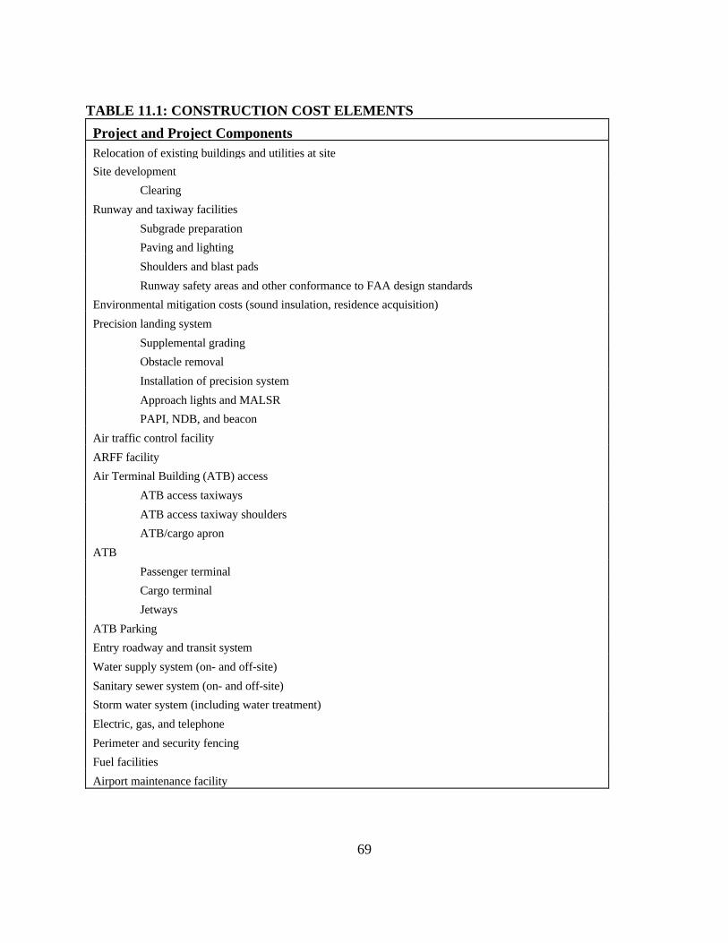
69

TABLE 11.1: CONSTRUCTION COST ELEMENTS

Project and Project ComponentsRelocation of existing buildings and utilities at site

Site development

Clearing

Runway and taxiway facilities

Subgrade preparation

Paving and lighting

Shoulders and blast pads

Runway safety areas and other conformance to FAA design standards

Environmental mitigation costs (sound insulation, residence acquisition)

Precision landing system

Supplemental grading

Obstacle removal

Installation of precision system

Approach lights and MALSR

PAPI, NDB, and beacon

Air traffic control facility

ARFF facility

Air Terminal Building (ATB) access

ATB access taxiways

ATB access taxiway shoulders

ATB/cargo apron

ATB

Passenger terminal

Cargo terminal

Jetways

ATB Parking

Entry roadway and transit system

Water supply system (on- and off-site)

Sanitary sewer system (on- and off-site)

Storm water system (including water treatment)

Electric, gas, and telephone

Perimeter and security fencing

Fuel facilities

Airport maintenance facility

70

11.3.2.4 Initial Training Cost. Some projects may require new operating skills that require thetraining of airport and/or airline staff, as well as additional training of pilots. Initial training costincludes travel, subsistence, and lodging associated with training, instructional cost, andcompensation of employees or persons being trained.

11.3.2.5 Transition Cost. Transition cost reflects the impact on airport operations of buildingand/or transitioning to the new project. This impact can be very large, particularly if theconstruction of the project leads to the temporary closure of major facilities of the airport. Arunway reconstruction project will lead to the total or partial closure of the runway itself, andmay cause the temporary closure of any runway intersecting with it. Disruption and delayassociated with the project may result in millions of dollars of additional costs to airlines, generalaviation users, passengers, and others using the airport, and must be measured and included as animportant cost element of the project.

Measurement of transition costs should be undertaken as a subset of the capacity simulationexercise described in section 10.4.1 of this guidance. Additional guidance on the subject oftransition costs associated with runway and facility reconstruction is provided in section 11.4.

11.3.3 Operations and Maintenance Cost (O&M): O&M costs are the recurring costs required tooperate and maintain the proposed investment project. The sponsor must demonstrate to FAAthat the proposed O&M regime will be adequate to sustain the project in good condition over thefull economic life assumed for the project. Expenses associated with O&M may occur annuallyor periodically every so many years.

11.3.3.1 Personnel Cost. Personnel cost is a major component of recurring O&M costs.Estimation of personnel cost is a multi-step process. The first step requires the determination ofthe annual labor hours required by type of skill. These hours should include not only directlabor, but such other items as recurring training, travel time, break time etc. Estimates for newsystems can be developed based on engineering data or previous experience with similar types ofundertakings. The second step in estimation of recurring labor costs is to adjust the requiredlabor hours for annual leave, sick leave, and other absences. The third step is to compute theeffective compensation rate (including fringe benefits) for each labor category. The final step isto translate annual labor requirements for each required skill into dollars by multiplying theannual labor hours required (from step 2) by the appropriate effective hourly compensation rate(as determined in step 3).

11.3.3.2 Materials. Materials consist of items as such as repair parts, small tools, lubricants,sealants, and other items which are consumed annually by the operation and maintenance of asystem.

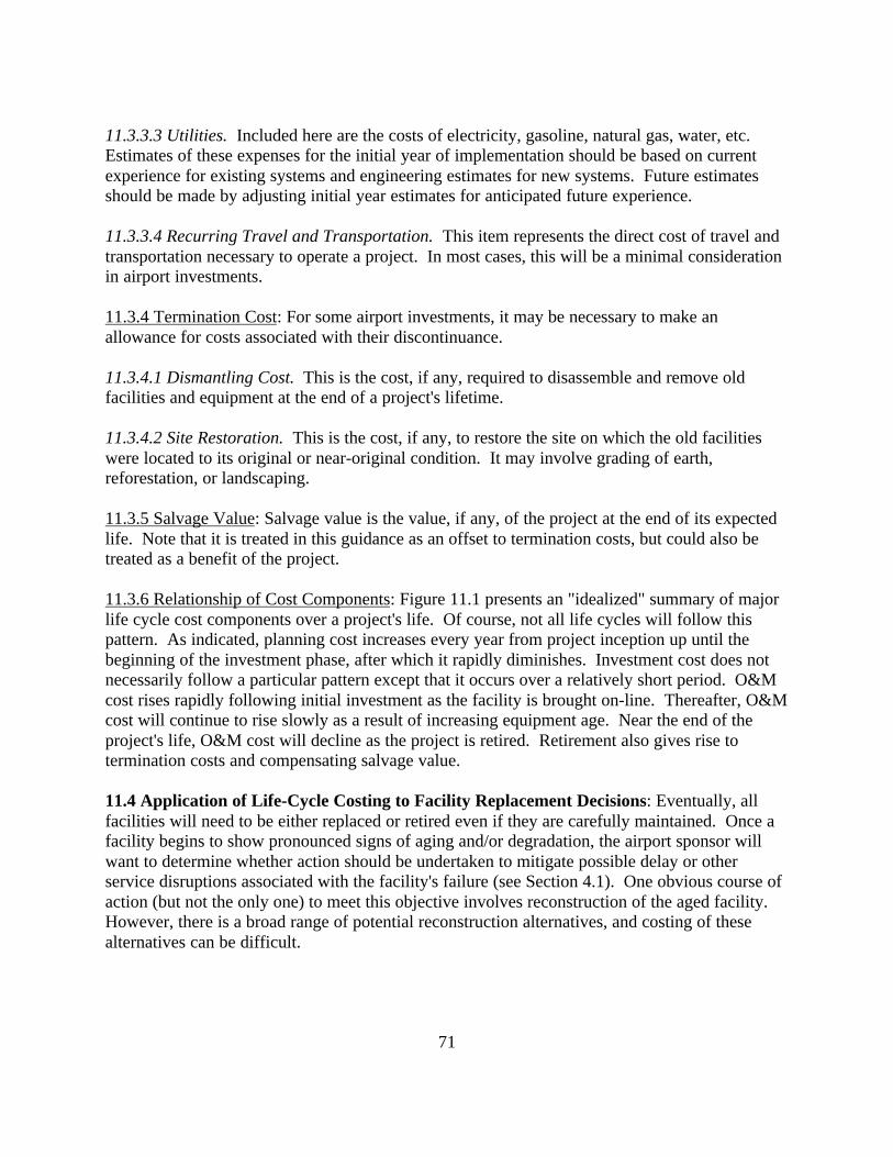
71

11.3.3.3 Utilities. Included here are the costs of electricity, gasoline, natural gas, water, etc.Estimates of these expenses for the initial year of implementation should be based on currentexperience for existing systems and engineering estimates for new systems. Future estimatesshould be made by adjusting initial year estimates for anticipated future experience.

11.3.3.4 Recurring Travel and Transportation. This item represents the direct cost of travel andtransportation necessary to operate a project. In most cases, this will be a minimal considerationin airport investments.

11.3.4 Termination Cost: For some airport investments, it may be necessary to make anallowance for costs associated with their discontinuance.

11.3.4.1 Dismantling Cost. This is the cost, if any, required to disassemble and remove oldfacilities and equipment at the end of a project's lifetime.

11.3.4.2 Site Restoration. This is the cost, if any, to restore the site on which the old facilitieswere located to its original or near-original condition. It may involve grading of earth,reforestation, or landscaping.

11.3.5 Salvage Value: Salvage value is the value, if any, of the project at the end of its expectedlife. Note that it is treated in this guidance as an offset to termination costs, but could also betreated as a benefit of the project.

11.3.6 Relationship of Cost Components: Figure 11.1 presents an "idealized" summary of majorlife cycle cost components over a project's life. Of course, not all life cycles will follow thispattern. As indicated, planning cost increases every year from project inception up until thebeginning of the investment phase, after which it rapidly diminishes. Investment cost does notnecessarily follow a particular pattern except that it occurs over a relatively short period. O&Mcost rises rapidly following initial investment as the facility is brought on-line. Thereafter, O&Mcost will continue to rise slowly as a result of increasing equipment age. Near the end of theproject's life, O&M cost will decline as the project is retired. Retirement also gives rise totermination costs and compensating salvage value.

11.4 Application of Life-Cycle Costing to Facility Replacement Decisions: Eventually, allfacilities will need to be either replaced or retired even if they are carefully maintained. Once afacility begins to show pronounced signs of aging and/or degradation, the airport sponsor willwant to determine whether action should be undertaken to mitigate possible delay or otherservice disruptions associated with the facility's failure (see Section 4.1). One obvious course ofaction (but not the only one) to meet this objective involves reconstruction of the aged facility.However, there is a broad range of potential reconstruction alternatives, and costing of thesealternatives can be difficult.

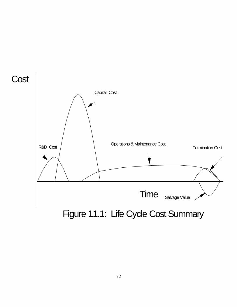
72

Cost

Time

Capital Cost

R&D CostOperations & Maintenance Cost

Termination Cost

Salvage Value

Figure 11.1: Life Cycle Cost Summary

73

11.4.1 Justification for Reconstruction Projects: The sponsor seeking to reconstruct a facilitymust show that its particular recommendation for reconstruction does the following:

• Generates net benefits relative to the base case; and• Produces greater net benefits than all other alternatives (e.g., relocating the facility,

building an alternate facility, etc.).

The base case for the above analysis should assume escalating O&M costs for the aged facility,followed by closure of the facility at some point when additional maintenance is no longer cost-effective.

11.4.2 Consideration of Degree of Reconstruction: There are several critical and interrelatedsteps that must be explicitly measured in costing potential reconstruction options:

• Timing of the reconstruction;• Degree of reconstruction needed;• Least-cost means of accomplishing a given degree of reconstruction (this analysis must

factor in the disruption costs to airport users during the reconstruction); and• Costs and benefits of associated projects in reconstruction decision.

11.4.2.1 Timing of Reconstruction. The sponsor must consider alternatives involving near-termreconstruction (within several years) and far-term reconstruction (e.g., in 10 years). Deferringreconstruction will lead to higher O&M expenses in the near-term and may lead to moreextensive damage of the aging facility and its subgrade, thus requiring a more extensivereconstruction in the future. In addition, if traffic is growing rapidly at the airport, deferringreconstruction may lead to greater traffic disruption once reconstruction is finally undertaken.Alternatively, if reconstruction can be deferred until a time when an already-planned substituteor additional facility becomes available, the cost of the deferred reconstruction alternative maybe much less than the cost of the immediate reconstruction alternative.

11.4.2.2 Degree of Reconstruction. The degree or extent of a potential reconstruction can behighly variable. In the case of a runway, reconstruction may involve the removal of a layer ofpavement with a subsequent replacement overlay. At the other extreme, a full-depthreconstruction of the runway and the subgrade could be undertaken.14 Both extremes (withappropriate intermediate levels) should be evaluated and costed.

14The overlay may last only half as long as the full depth reconstruction, inwhich case the cost of the overlay option would need to reflect two separateoverlays to be comparable to the full depth reconstruction.

74

11.4.2.3 Least-Cost Means of Reconstruction. The cost of a given reconstruction option (e.g.,partial pavement replacement) can vary significantly based on the assumptions concerning thereconstruction method and schedule. In many cases it is possible to reconstruct a runway atnight or in segments, thus keeping it partially open to airport users (who therefore incur lowerdisruption cost) but at higher cost for labor and materials. Alternatively, if the runway is closedcompletely to enable full-time reconstruction, physical construction costs will be lower butdisruption cost to airport users will be higher. Consequently, it is essential that a complete rangeof reconstruction schedules be explored and costed.

Impacts on users caused by reconstruction should be estimated using appropriate capacitymodels (see Section 10.4.1). In general, delay or other disruption associated with thereconstruction option must be assigned a value and considered along with other measured costs.

11.4.3.4 Consideration of Linked Reconstruction Projects. A capacity project may be proposedprincipally to accommodate airport users during the reconstruction of a separate item of airportinfrastructure. In such cases, the two projects (the reconstruction project and the facilityintended to accommodate disruption associated with it) must be linked into one overall projectand subjected to one BCA.

75

Section 12: MULTI-PERIOD ECONOMIC DECISION CRITERIA

12.1 Requirement for Multi-Period Analysis: The emphasis of this guidance until now hasbeen on the fullest practical identification, quantification, and monetization of benefits and costsfor various project types. These benefits and costs are developed in constant dollars for a limitednumber of focus years. This section of the guidance will accomplish three principal objectives:

• Provide instructions on how to interpolate/extrapolate focus year benefits and costs toeach year of the project's construction and/or operating life;

• Describe analytical methods for quantifying and comparing multi-period benefit and coststreams; and

• Recommend appropriate methods for selecting optimal alternatives.

A brief discussion on the measurement of optimal timing for investments is also provided.

12.2 Creation of Multi-Period Benefit Series: With the exception of project capital costs(which are developed for each year of the construction period), benefit and cost data in theprevious sections are developed for several levels of future demand (measured in terms ofenplanements and/or operations) that correspond to selected project years, called focus years.These years are selected from the beginning, middle, and late stages of the project's expected life.

The limitation of benefit and cost measurements to focus years is largely a function of theexcessive level of effort and expense that would be required to simulate capacity benefits foreach project year. However, BCA requires that benefits and costs be developed for each year ofthe project life. Thus, the analyst must interpolate and/or extrapolate benefit and cost results ofthe focus years to those years and traffic levels for which benefits and costs were not directlymeasured.

The principal benefit of most capacity projects will be delay reduction. As such, selection offocus years should be done in a manner that allows the analyst to approximate the comparativedelay trends of the base case and its alternatives. Section 10.4.1 provides a detailed methodologyfor selection and adjustment of focus years to enable a good linear approximation of curvilineardelay growth trends.

If focus years are properly selected, the interpolation of benefits between two points can be doneby a simple per operation or per passenger pro-ration process. That is, if aircraft operating delaysavings of an alternative relative to the base case are 1,000 hours at 500,000 operations, and2,000 hours at 550,000 operations, then it may be assumed that savings would be 1,500 hours at525,000 operations. Moreover, to the extent that other benefits attributable to the project arerelated to operations and/or passenger levels, this linear pro-ration approach is also appropriate.

Assuming that one of the focus years selected for the project corresponds to a demand level atthe end of the project's projected life, the need to extrapolate benefits beyond this year is limited.However, to conform with the guidance in Section 8.3, it will be necessary to extrapolate project

76

benefits from the final focus year by at least 5 years to accommodate analysis of optimal timingof projects. In this case, extrapolation of benefits from the final focus year should occur at thesame rate of benefit per operation (or passenger) as measured between the next-to-final and finalfocus years (provided the delay benefit level does not exceed 20 minutes per operation--seeSection 10.4.1.)

12.3 Creation of Multi-Period Cost Series: O&M cost data will generally grow at a constantper operation or per passenger unit rate and can safely be pro-rated on this basis. In some cases,the cost of periodic maintenance events may be scheduled for discreet years.

12.4 Conversion of Benefit and Cost Series to Present Value: Most airport investmentsinvolve the expenditure of large blocks of resources at the outset of the project in return for anannual (usually rising) flow of benefits to be realized in the future. Although these benefits andcosts are in the form of dollars, year-to-year benefits and costs cannot simply be summed intototals and then compared. Rather, the BCA must take into account the fact that dollars paid outor earned in the near-term are worth more in "present value" than are dollars paid out or earnedin the far-term. The process of converting future cash flows into present value is calleddiscounting.

The opportunity cost of money accounts for the need to discount dollar amounts to account forthe passage of time. Another factor that may affect the perception of the value of future revenuestreams--risk and uncertainty--should be dealt with explicitly in the BCA and not throughdiscounting future dollar streams.

12.4.1 Opportunity Cost of Capital: The opportunity cost of capital reflects the fact that, evenwithout inflation, the present value (the value today) of a dollar to be received a year from now isless than the value of a dollar in-hand today. This outcome can be easily understood from thestandpoint of lost revenue-earning opportunity. A dollar in-hand can be invested immediately inan interest-bearing account (or some other investment instrument) and earn interest for a periodof one year. A dollar to be received one year from now cannot earn income for the investorduring this period. Thus, the BCA must account for the opportunity cost of capital.

12.4.2 Inflation: Inflation reflects the diminishing value of a dollar from year to year as measuredin the real resources and services for which it can be exchanged. Although inflation is animportant issue in investment analysis, FAA recommends that benefits and costs of projects bevalued in terms of constant study year dollars (see Sections 10.5.1 and 11.2.6). As such, the roleof inflation is already removed from the benefit and cost streams developed in Sections 10 and11 of this guidance and no discounting of future revenue streams for inflation is required.

12.4.3 Risk: Investors will frequently discount future revenues more severely if these revenuesare characterized by a high degree of risk and uncertainty. Consequently, market interest ratesassociated with risky bonds are substantially higher than those for secure bonds. However, theU.S. Office of Management and Budget states that risk and uncertainty should be dealt with

77

explicitly in the BCA using sensitivity analysis, probability distributions, and expected values--not through the discount rate applied to future monetary flows (see Section 13).

12.5 Discount Rate: Discounting requires the division of an annual discount rate into futurebenefits and costs. The annual discount rate (also known as the marginal rate of return ofcapital) represents the prevailing level of capital productivity that can be achieved at anyparticular time by investing resources, i.e., the opportunity cost. Because FAA recommends theuse of constant dollar cash streams, the discount rate should be net of inflation. This net-of-inflation rate is called the real discount rate.

The Office of Management and Budget (OMB) of the Executive Office of the President of theUnited States specifies appropriate real discount rates for investments of Federal funds inCircular No. A-94 (October 29, 1992). The real discount rate relevant to all airport projects to befunded with Federal grant funds is 7 percent.

12.6 Basic Discounting Methodology: The present value (PV) of a future cost or benefit for agiven year “n” is determined by the following formula:

where:

V = future value in year n in constant dollarsr = annual real discount raten = number of years from the base year (study year)

When whole numbers are used for "n", the above formula assumes that all costs and benefits in ayear occur at the end of the year. A mid-year accrual can be simulated by the use of half valuesfor "n" (i.e., n = ½, 1½, 2½, etc.). Finally, a discounting formula can be applied which assumescontinuous accrual of costs and benefits over the course of a year.15

From a practical point of view, the mid-point and continuous discounting procedures are aboutthe same. Either can be used to approximate the continuous characteristic of benefit and coststreams. Also, there is not a large difference between the end-of-period discounting and eithermid-period or continuous discounting--less than 4 percent at a 7 percent discount rate. Therelatively small changes produced by different discounting procedures suggests that, with respectto project evaluation, any of the methods is acceptable.

15Present value tables, located in various financial text books, can also beused.

1-1 )r+(1

V=PV

n

n2

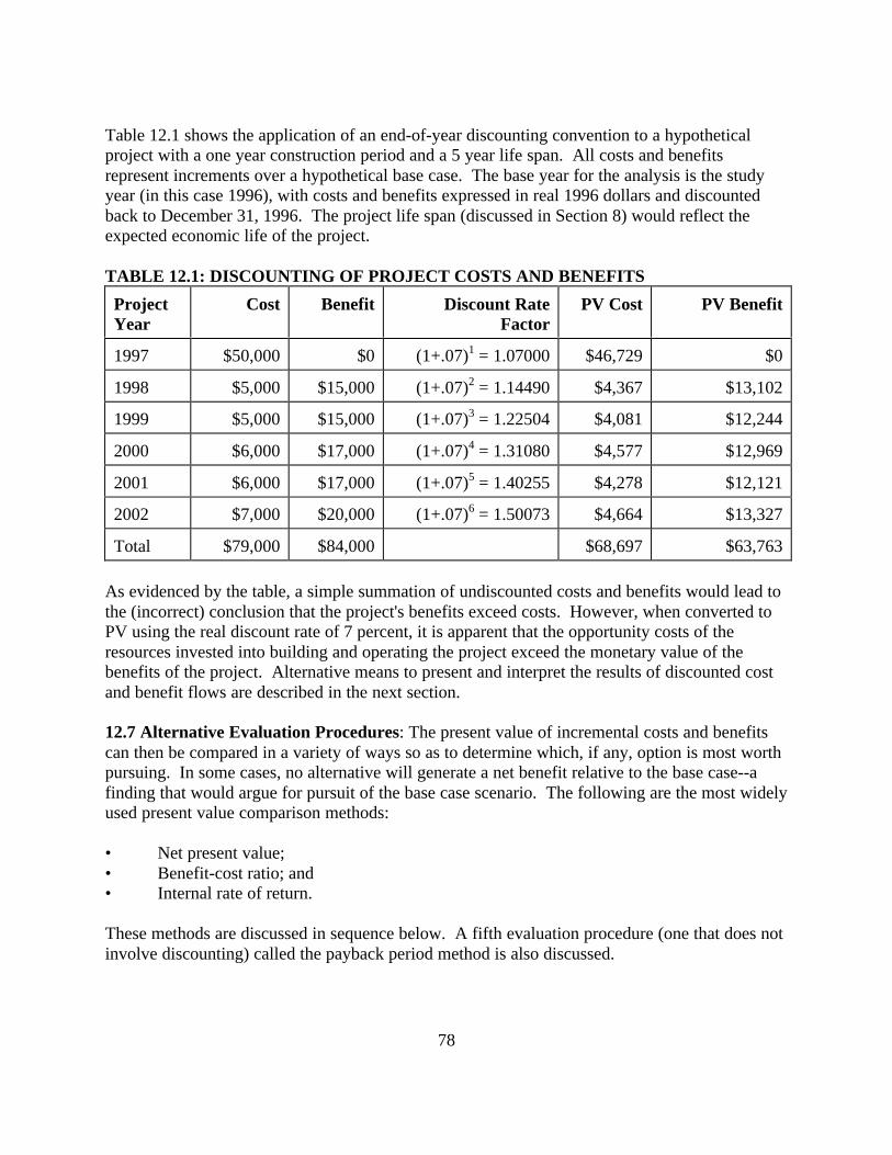
78

Table 12.1 shows the application of an end-of-year discounting convention to a hypotheticalproject with a one year construction period and a 5 year life span. All costs and benefitsrepresent increments over a hypothetical base case. The base year for the analysis is the studyyear (in this case 1996), with costs and benefits expressed in real 1996 dollars and discountedback to December 31, 1996. The project life span (discussed in Section 8) would reflect theexpected economic life of the project.

TABLE 12.1: DISCOUNTING OF PROJECT COSTS AND BENEFITS

ProjectYear

Cost Benefit Discount RateFactor

PV Cost PV Benefit

1997 $50,000 $0 (1+.07)1 = 1.07000 $46,729 $0

1998 $5,000 $15,000 (1+.07)2 = 1.14490 $4,367 $13,102

1999 $5,000 $15,000 (1+.07)3 = 1.22504 $4,081 $12,244

2000 $6,000 $17,000 (1+.07)4 = 1.31080 $4,577 $12,969

2001 $6,000 $17,000 (1+.07)5 = 1.40255 $4,278 $12,121

2002 $7,000 $20,000 (1+.07)6 = 1.50073 $4,664 $13,327

Total $79,000 $84,000 $68,697 $63,763

As evidenced by the table, a simple summation of undiscounted costs and benefits would lead tothe (incorrect) conclusion that the project's benefits exceed costs. However, when converted toPV using the real discount rate of 7 percent, it is apparent that the opportunity costs of theresources invested into building and operating the project exceed the monetary value of thebenefits of the project. Alternative means to present and interpret the results of discounted costand benefit flows are described in the next section.

12.7 Alternative Evaluation Procedures: The present value of incremental costs and benefitscan then be compared in a variety of ways so as to determine which, if any, option is most worthpursuing. In some cases, no alternative will generate a net benefit relative to the base case--afinding that would argue for pursuit of the base case scenario. The following are the most widelyused present value comparison methods:

• Net present value;• Benefit-cost ratio; and• Internal rate of return.

These methods are discussed in sequence below. A fifth evaluation procedure (one that does notinvolve discounting) called the payback period method is also discussed.

79

12.7.1 Net Present Value (NPV): The net present value (NPV) method requires that analternative meet the following criteria to warrant investment of funds:

• Have a positive NPV; and• Have the highest NPV of all tested alternatives.

The first condition insures that the alternative is worth undertaking relative to the base case, e.g.,it contributes more in incremental benefits than it absorbs in incremental costs. The secondcondition insures that maximum benefits (in a situation of unrestricted access to capital funds)are obtained.

The formula for the calculation of NPV is as follows:

where:

B = future annual benefits in constant dollarsC = future annual costs inconstant dollarsr = annual real discount ratek = number of years from the base year over which the project will be evaluatedt = an index running from 0 to k representing the year under consideration

As an illustration of the application of NPV, consider the example in Table 12.2. Threeinvestment options are presented. The values for benefits and costs of each are incremental tothe base case, in 1996 dollars, and are discounted to the present at the OMB-prescribed realdiscount rate of 7 percent.

Alternative A does not have a positive NPV and should not be pursued relative to the base case.Both alternatives B and C have positive NPVs, indicating either option would be preferred to thebase case. However, alternative C has the highest NPV, making it the best alternative to pursue.

NPV is the most widely-used and theoretically-accurate economic method for selecting amonginvestment alternatives, and should be used for all analyses prepared for the FAA'sconsideration. However, NPV does have certain conceptual and analytical limitations, whichmakes consideration of other present value evaluation methods appropriate in some instances.

2-1 )r+(1

C - )r+(1

B = )r+(1

)C-(B = NPV

tt

k

0=tt

tk

0=ttt

k

0=t

2∑∑∑

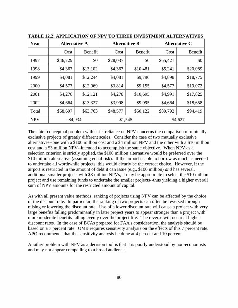
80

TABLE 12.2: APPLICATION OF NPV TO THREE INVESTMENT ALTERNATIVES

Year Alternative A Alternative B Alternative C

Cost Benefit Cost Benefit Cost Benefit

1997 $46,729 $0 $28,037 $0 $65,421 $0

1998 $4,367 $13,102 $4,367 $10,481 $5,241 $20,089

1999 $4,081 $12,244 $4,081 $9,796 $4,898 $18,775

2000 $4,577 $12,969 $3,814 $9,155 $4,577 $19,072

2001 $4,278 $12,121 $4,278 $10,695 $4,991 $17,825

2002 $4,664 $13,327 $3,998 $9,995 $4,664 $18,658

Total $68,697 $63,763 $48,577 $50,122 $89,792 $94,419

NPV -$4,934 $1,545 $4,627

The chief conceptual problem with strict reliance on NPV concerns the comparison of mutuallyexclusive projects of greatly different scales. Consider the case of two mutually exclusivealternatives--one with a $100 million cost and a $4 million NPV and the other with a $10 millioncost and a $3 million NPV--intended to accomplish the same objective. When NPV as aselection criterion is strictly applied, the $100 million alternative would be preferred over the$10 million alternative (assuming equal risk). If the airport is able to borrow as much as neededto undertake all worthwhile projects, this would clearly be the correct choice. However, if theairport is restricted in the amount of debt it can issue (e.g., $100 million) and has several,additional smaller projects with $3 million NPVs, it may be appropriate to select the $10 millionproject and use remaining funds to undertake the smaller projects--thus yielding a higher overallsum of NPV amounts for the restricted amount of capital.

As with all present value methods, ranking of projects using NPV can be affected by the choiceof the discount rate. In particular, the ranking of two projects can often be reversed throughraising or lowering the discount rate. Use of a lower discount rate will cause a project with verylarge benefits falling predominantly in later project years to appear stronger than a project withmore moderate benefits falling evenly over the project life. The reverse will occur at higherdiscount rates. In the case of BCAs prepared for FAA's consideration, the analysis should bebased on a 7 percent rate. OMB requires sensitivity analysis on the effects of this 7 percent rate.APO recommends that the sensitivity analysis be done at 4 percent and 10 percent.

Another problem with NPV as a decision tool is that it is poorly understood by non-economistsand may not appear compelling to a broad audience.

81

12.7.2 Benefit-Cost Ratio: The benefit-cost ratio is defined as the present value of benefitsdivided by the present value of costs. The formula for the calculation of the benefit-cost ratio isas follows:

A proposed activity with a ratio of discounted benefits to costs of 1 or more will return at least asmuch in benefits as it costs to undertake--indicating that the activity is worth undertaking. In thecase of the investment alternatives developed in Table 12.2, the benefit-cost ratios foralternatives A, B, and C would be 0.93, 1.03, and 1.05, respectively.

The principal advantage of the benefit-cost ratio is that it is intuitively understood by mostpeople. Moreover, this method does provide a correct answer as to which objectives should beundertaken--defined as those with ratios greater than or equal to unity. However, it often fails toanswer correctly the question of how to accomplish the objectives most effectively, particularlywhen comparing mutually exclusive projects of different scale or different levels of capitalintensity and operating expense.

The difficulty associated with project scale is the flip side of the scale problem associated withNPV. In the case described above for NPV (where a $100 million investment would yield a$4 million NPV and a $10 million investment would yield a $3 million NPV) the benefit-costratios would be 1.04 and 1.3, respectively. Reliance on these ratios would lead to the choice ofthe $10 million investment. However, as already noted, only in a situation when an airport'sability to issue debt is constrained would the choice of the $10 million investment be appropriate(assuming equal risk). Where an airport is able to raise ample capital for its investment needs,the preferred project would be the $100 million one.

The benefit-cost ratio cannot properly compare capital intensive projects with others that havesignificant operating expenses. An example of this is shown in Table 12.3.16

16Adapted from De Neufville.

3-1

)r+(1C

)r+(1B

= B/C

tt

k

0=t

tt

k

0=t 2

∑

∑

where:

Bt = future annual benefits in constant dollarsCt = future annual costs inconstant dollarsr = annual real discount ratet = an index running from 0 to k representing the year under consideration

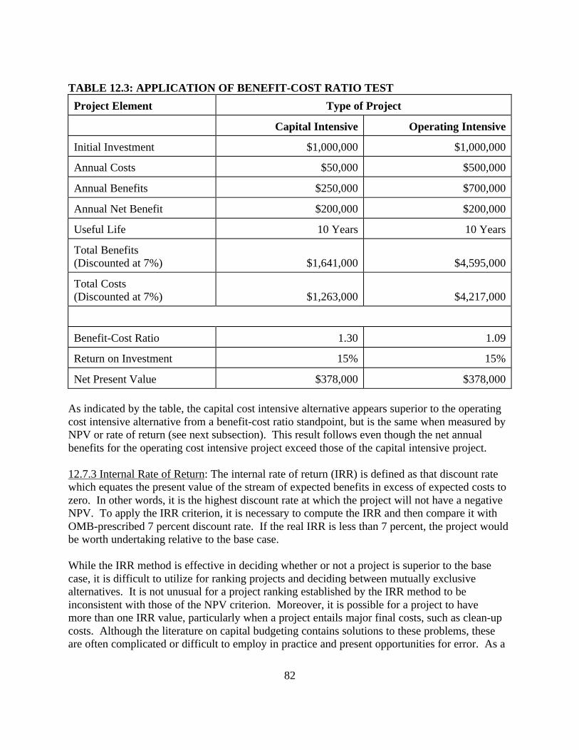
82

TABLE 12.3: APPLICATION OF BENEFIT-COST RATIO TEST

Project Element Type of Project

Capital Intensive Operating Intensive

Initial Investment $1,000,000 $1,000,000

Annual Costs $50,000 $500,000

Annual Benefits $250,000 $700,000

Annual Net Benefit $200,000 $200,000

Useful Life 10 Years 10 Years

Total Benefits(Discounted at 7%) $1,641,000 $4,595,000

Total Costs(Discounted at 7%) $1,263,000 $4,217,000

Benefit-Cost Ratio 1.30 1.09

Return on Investment 15% 15%

Net Present Value $378,000 $378,000

As indicated by the table, the capital cost intensive alternative appears superior to the operatingcost intensive alternative from a benefit-cost ratio standpoint, but is the same when measured byNPV or rate of return (see next subsection). This result follows even though the net annualbenefits for the operating cost intensive project exceed those of the capital intensive project.

12.7.3 Internal Rate of Return: The internal rate of return (IRR) is defined as that discount ratewhich equates the present value of the stream of expected benefits in excess of expected costs tozero. In other words, it is the highest discount rate at which the project will not have a negativeNPV. To apply the IRR criterion, it is necessary to compute the IRR and then compare it withOMB-prescribed 7 percent discount rate. If the real IRR is less than 7 percent, the project wouldbe worth undertaking relative to the base case.

While the IRR method is effective in deciding whether or not a project is superior to the basecase, it is difficult to utilize for ranking projects and deciding between mutually exclusivealternatives. It is not unusual for a project ranking established by the IRR method to beinconsistent with those of the NPV criterion. Moreover, it is possible for a project to havemore than one IRR value, particularly when a project entails major final costs, such as clean-upcosts. Although the literature on capital budgeting contains solutions to these problems, theseare often complicated or difficult to employ in practice and present opportunities for error. As a

83

consequence, it is not recommended that the IRR method be used to evaluate airport projects forwhich AIP funds will be requested.

12.7.4 Payback Period: The payback period measures the number of years required for netundiscounted benefits to recover the initial investment in a project. One characteristic of thisevaluation method is that it favors projects with near-term (and more certain) benefits. However,the payback period method fails to consider benefits beyond the payback period. Nor does itprovide information on whether an investment is worth undertaking in the first place. Althoughoften used in business applications, the payback period method is not appropriate for analysesconducted to justify the investment of AIP or other U.S. government funds.

12.8 Evaluation of Optimal Project Timing: The issue of optimal project timing is frequentlyignored in economic analysis, but is particularly important in the case of large infrastructureprojects typical of airports. In some cases, BCA may reveal that a greater net benefit can berealized if a project is deferred for several years rather than implemented immediately. Such asituation has a higher likelihood of occurring if the following conditions are met:

• The project benefit stream is heavily weighted to the later years of the project life;• The project is characterized by large, up-front capital costs; and• Capital and land cost escalation can be contained through land banking or other means.

Section 8.3 of this guidance recommended that benefit and cost figures be developed for a periodof at least 5 years beyond the estimated project life. NPV can then be calculated for the projectbeginning in year X and year X+5, each with a benefit stream lasting the same number of years(e.g., 20 years beyond the completion of construction). Thus, the project NPV would becalculated for the following two time scenarios:

To resolve the issue of optimal timing, the NPV for each alternative should be measured for boththe current and delayed time scenarios.

12.9 Selection of Best Alternative: Given equal risk and uncertainty, FAA recommends that thealternative/time scenario with the largest positive NPV be given primary consideration as thepreferred course of action. In the case of Table 12.4, the preferred course of action would be

4-1 )r+(1

)C-(B = NPV

tt

k

0=t

2∑

5-1 )r+(1

)C-(B = NPV

tt

5+k

=t

25

∑

84

alternative C, but with project implementation delayed by 5 years.17 If this course of action isselected, it would be appropriate to revisit the BCA within 5 years to make sure that data andassumptions contained in it are still valid.

TABLE 12.4: BCA RESULTS FOR THREE ALTERNATIVES

Option NPV With ConstructionBeginning in Year t=1

NPV With ConstructionBeginning in Year t=6

Alternative A $5 million $10 million

Alternative B $1 million $1.5 million

Alternative C $8 million $14 million

Of course, not all alternatives will have equal certainty. Alternative A in year t+1 may be muchless subject to cost overruns than alternative C in year t+5. The issue of sensitivity and itsimpact on investment decisions is described in the next section of this guidance.

17 This assumes that it is not feasible to do Alternative C in Year t=1 andextend its life by 5 years, assuming Bi > Ci for i=1,..,5.

85

Section 13: UNCERTAINTY

13.1 Need to Address Uncertainty: The outcome of a BCA will depend on numerous estimates,forecasts, assumptions, and approximations of reality. Each of these factors has the potential tointroduce error into the results. The importance of such errors in affecting the outcome of theBCA must be known to the decision-maker if informed decisions are to be made and confidenceplaced in such decisions. Moreover, the degree of uncertainty associated with each alternative isitself a factor to be considered in selecting between competing alternatives.

13.2 Characterizing Uncertainty: The treatment of uncertainty must be guided by theprinciples of full disclosure and transparency. Data, models, and their implications for riskassessment should be identified. Inferences and assumptions should be identified and evaluatedexplicitly, together with adequate justifications for choices made, and assessments of the effectsof these choices on the BCA.

13.3 Sensitivity Analysis: Sensitivity analysis is an important tool for evaluating the impacts ofuncertainty on proposed investment projects. The basic approach is to vary key assumptions,estimates, and forecasts systematically over appropriate ranges and observe the impact on theresults. For certain items, the impact may be insignificant while for others it may be quite large.In some cases the relative desirability of competing alternatives may be altered while in others itwill not be.

13.3.1 Probability Distributions: The actual procedure for varying a parameter depends onwhether or not it may be described by a known probability distribution. If it can be so described,probability statements can be made about each value selected and the outcome of the analysis.Such an approach is known by convention as risk analysis.

If the probability distribution for each parameter is not known, alternative values of theparameter are selected over a range over which it is known or believed reasonable for it to vary.Probability statements regarding the likely occurrence of any particular value of the parameterare not possible. This approach is known as uncertainty analysis.

13.3.2 Methods of Sensitivity Analysis: There are several ways in which the analysis can beaccomplished. Each depends on how the key assumptions, estimates, and forecasts are varied.One procedure is to vary only one at a time, holding the others constant so as to determine theindependent, or partial, effect of this parameter. This procedure is known as a one variableuncertainty test. A second procedure is to vary two parameters simultaneously and is known as atwo variable uncertainty test.

Similarly, three, four and more variable uncertainty tests can be constructed. These can easilyproduce large amounts of data and require the decision maker to consider an excessively largenumber of outcomes. An alternative is to allow all parameters to vary together in severalpredetermined patterns, each representing a relevant probable future state of affairs. This

86

procedure is known as alternative scenario analysis and makes use of probabilistic or "stochastic"computer simulation techniques.

13.3.2.1 One Variable Test. This procedure should be applied to the major cost and benefitcomponents of each alternative. Its primary purpose is to identify the sensitivity of the NPV ofeach alternative to changes in value of each component. This permits additional effort to bedevoted to improving the reliability of estimates for those components to which the results aresensitive. Where reliability cannot be improved, it puts the decision-maker on notice as topotential weaknesses of the BCA.

To carry out the one variable tests, the NPV of each alternative must be recalculated for differentvalues of any one particular component while others are held constant. The range of valuesshould extend over those that can reasonably be expected to prevail. Where a probabilitydistribution for the component of interest is known, this range may be established by aconfidence interval (usually 90 to 95 percent). Where such a distribution is unknown, the rangeshould extend from the smallest to the largest value that could reasonably by expected to occur.The process should be repeated for each major component to be tested.

Once these computations have been completed, the problem arises as to how to display theresults. If only a small number of components were tested, a tabular display may be appropriate.If more components were varied, a graphical display is often useful. Consider the followingexample of a new runway. Estimates indicate that installation of a new runway will generatebenefits and costs over a 20 year economic life with present values of $45 million and$35 million, respectively, for a net present value of $10 million. These estimates are based onthree basic forecast variables: traffic growth; economic life; and construction cost. Figure 13.1indicates the impact on NPV that will occur if each of these items is allowed to vary over a rangeof plus or minus 100 percent of its value while the others are held constant.

As can be seen, increases in construction costs above 55 percent will result in a negative NPVindicating that the project should not be undertaken. Shortening the economic life by about50 percent will also result in the NPV becoming negative. Changes in traffic growth will notaffect the desirability of the project unless growth is about 90 percent less than predicted. Fromthis information, the decision-maker can conclude that the project will have a positive NPVunless there are substantial changes in the key variables.

13.3.2.2 Two Variable Test. The one variable test permits examination of one factor holding allothers constant. However, it may be useful to let two factors change at the same time,particularly if such changes may be expected to occur together. Or it may be necessary todetermine the extent to which a change in one factor can be offset by a change in another.

As indicated in Figure 13.2, a different curve relating NPV to economic life may be constructedfor each different level of construction spending. For any given NPV, it is shown

87

Net PresentValue($Millions)

Percentage Change inVariable

-100 -50 0 10050

0

25

-15

Construction

Traffic Growth

Economic Life

Figure 13.1: One Variable Uncertainty Test

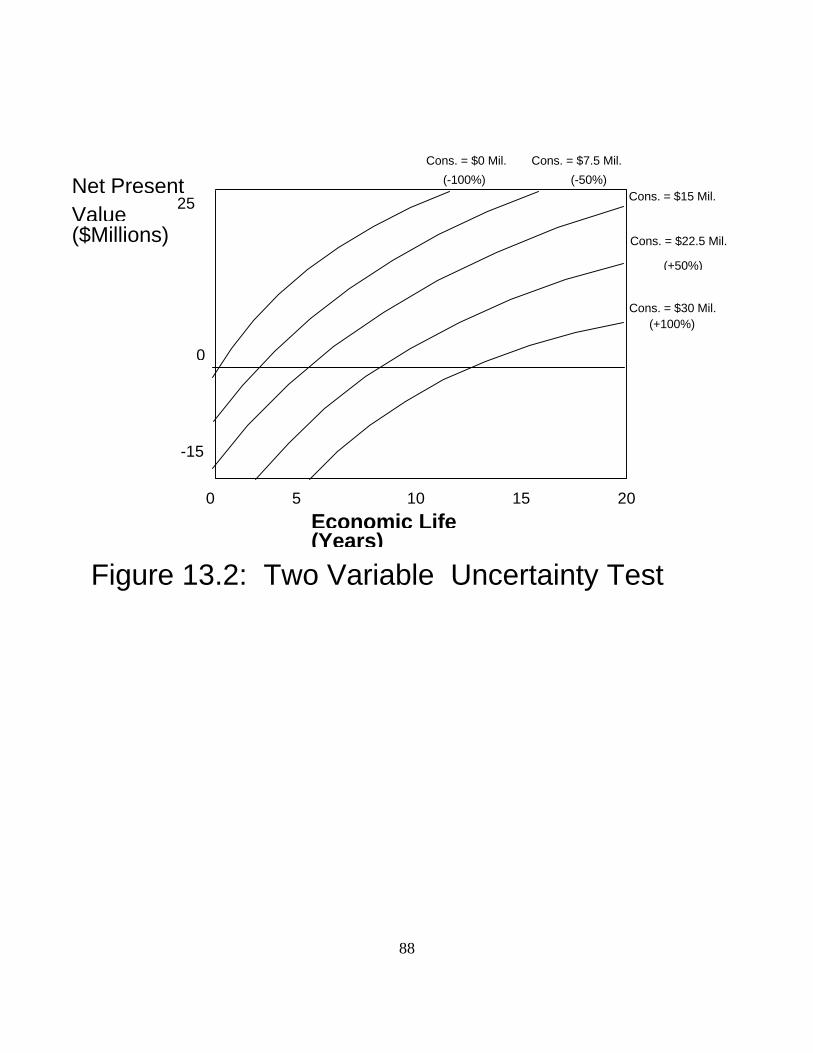
88

Net PresentValue($Millions)

Economic Life(Years)

0 5 10 2015

0

25

-15

Figure 13.2: Two Variable Uncertainty TestTTestUncertainty

Cons. = $30 Mil. (+100%)

Cons. = $22.5 Mil.

(+50%)

Cons. = $15 Mil.

Cons. = $7.5 Mil.

(-50%)

Cons. = $0 Mil.

(-100%)

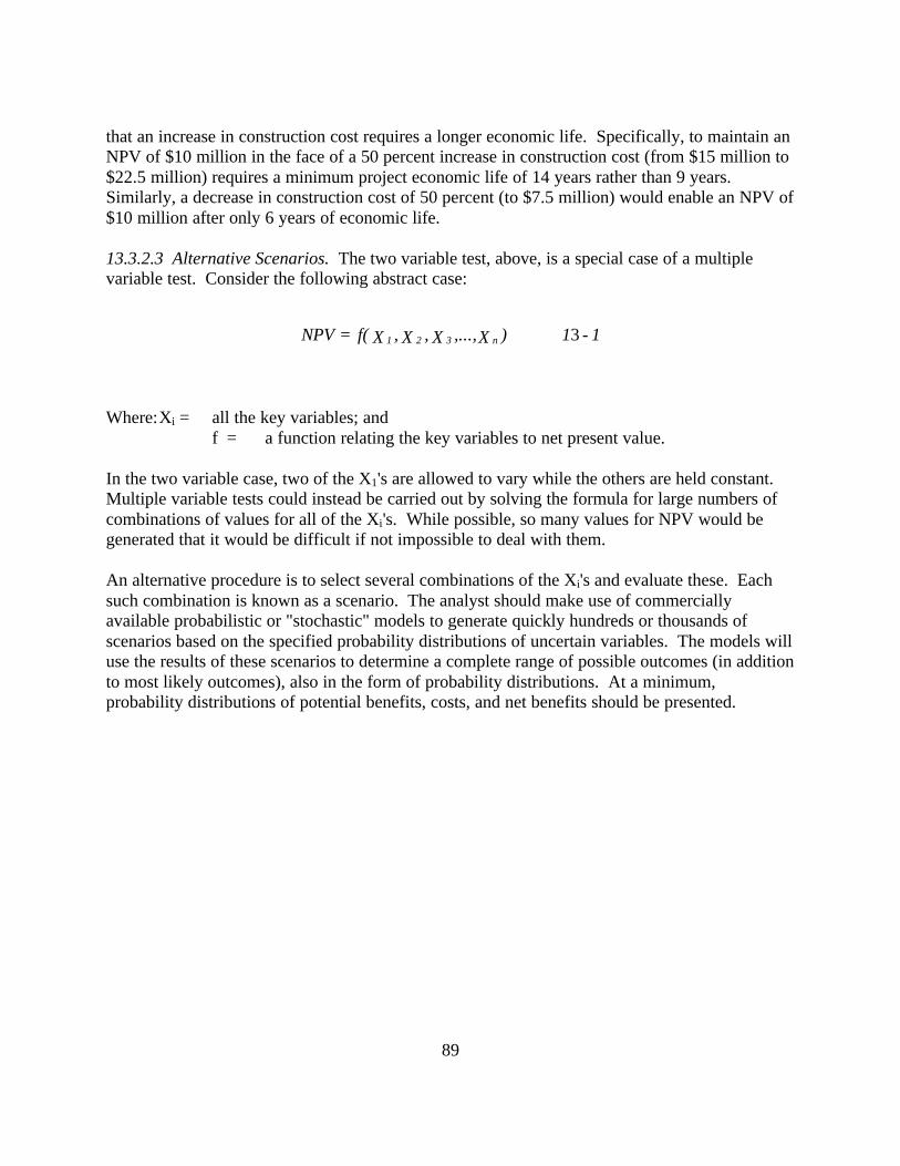
89

that an increase in construction cost requires a longer economic life. Specifically, to maintain anNPV of $10 million in the face of a 50 percent increase in construction cost (from $15 million to$22.5 million) requires a minimum project economic life of 14 years rather than 9 years.Similarly, a decrease in construction cost of 50 percent (to $7.5 million) would enable an NPV of$10 million after only 6 years of economic life.

13.3.2.3 Alternative Scenarios. The two variable test, above, is a special case of a multiplevariable test. Consider the following abstract case:

Where:Xi = all the key variables; andf = a function relating the key variables to net present value.

In the two variable case, two of the X1's are allowed to vary while the others are held constant.Multiple variable tests could instead be carried out by solving the formula for large numbers ofcombinations of values for all of the Xi's. While possible, so many values for NPV would begenerated that it would be difficult if not impossible to deal with them.

An alternative procedure is to select several combinations of the Xi's and evaluate these. Eachsuch combination is known as a scenario. The analyst should make use of commerciallyavailable probabilistic or "stochastic" models to generate quickly hundreds or thousands ofscenarios based on the specified probability distributions of uncertain variables. The models willuse the results of these scenarios to determine a complete range of possible outcomes (in additionto most likely outcomes), also in the form of probability distributions. At a minimum,probability distributions of potential benefits, costs, and net benefits should be presented.

1-1 )X,...,X ,X ,Xf( = NPV n321 3

90

Section 14: SELECTION OF OPTIMAL PROJECT

14.1 Consideration of All Information: The final outcome of the BCA process is arecommendation on the best course of action, if any, to attain the proposed objective. Therecommendation of the appropriate alternative will depend on measured benefits and costs,consideration of hard-to-quantify benefits and costs, and sensitivity of results to uncertainty.

14.2 Net Present Value: FAA recommends that the alternative with the largest positive NPV (ifany) be given primary consideration as the preferred course of action. Note that the operativeword here is “consideration”. The recommend alternative is not automatically the one which hasthe largest positive NPV. All relevant data such as hard-to-quantify benefits and costs anduncertainty must also be considered in deciding on the preferred alternative

14.3 Hard-To-Quantify Benefits and Costs: In selecting between alternatives that haveapproximately equal NPVs, particular weight should be assigned to the alternative with thepreponderance of qualitatively described benefits. Moreover, the airport sponsor may believethat a lesser-ranked project from an NPV perspective has very important hard-to-quantifybenefits that would make it preferable to other alternatives. In this case, the sponsor may selectthe lesser-ranked project provided that the reasons for selecting this project are clearly described.

14.4 Uncertainty: Sensitivity analysis may reveal that an alternative with a lower NPV rankingalso has a much lower risk of failing to realize net positive benefits. In such cases, the projectsponsor may justify the selection of the lower-ranked alternative, particularly if potential failureof the higher ranked alternatives would lead to large economic losses. Comparison ofalternatives from the standpoint of risk will be greatly facilitated by the generation of probabilitydistributions around expected NPVs.

A-1

Appendix A: TREATMENT OF INFLATION

[Note: This appendix is taken from CHAPTER 7. INFLATION in Economic Analysis ofInvestment and Regulatory Decisions -- Revised Guide, Federal Aviation Administration, ReportFAA-APO-98-4, dated January 1998.]

A.1 Introduction

The performance of economic analysis requires that benefits and costs be measured. Theyardstick of measurement is the dollar. This yardstick must remain unchanged for all quantitiesmeasured if resulting measurements are to be meaningful and comparable with each other. Butthe value of the dollar is rarely constant from one year to the next. Changes in the prices ofgoods and services continuously effect the purchasing power of the dollar. This chapter dealswith how to manage changes in the value of the dollar over time in order that benefits and costsoccurring in different years may be consistently measured.

A.2 Price Changes

This section is divided into two parts: measuring inflation and measuring price changes forspecific commodities. Inflation may be defined as a change in the general price level -- this is achange in the average price of all goods and services produced in the economy or which areregularly purchased by a defined buyer or class of buyers. It is conceptually distinct from thechange in the price of any specific commodity, which most likely will be changing at a differentrate than the price level or even moving in the opposite direction.

A.2.1 Measuring Inflation

Changes in the value of the dollar over time are measured using an index number. For theoverall U.S. economy, a broadly based index representing the price of all goods and servicessuch as the Gross Domestic Product (GDP) Implicit Price Deflator is commonly used. Whenconsidering the goods and services typically bought by a subset of purchasers, such ashouseholds, a more narrowly defined index is typically employed. Such numbers are a measureof relative value. They indicate the price of the group of goods and services of interest in oneyear relative to some other year. By convention, index numbers are usually computed as theratio of the price of the goods and services of interest in one year divided by their price in thebase year. The resulting ratio is then multiplied by 100 to produce the index number. Repeatingthe process for a number of years results in a series of index numbers.

To illustrate the methodology of working with index numbers, consider the two price measuresfor GDP reported in Table A.1: The GDP Implicit Price Deflator and the GPD Chain-Type PriceIndex. Both measures are currently published by the Bureau of Economic Analysis of theDepartment of Commerce. Because the two series differ only slightly, it is appropriate to useeither. The following examples make reference to the deflator series.

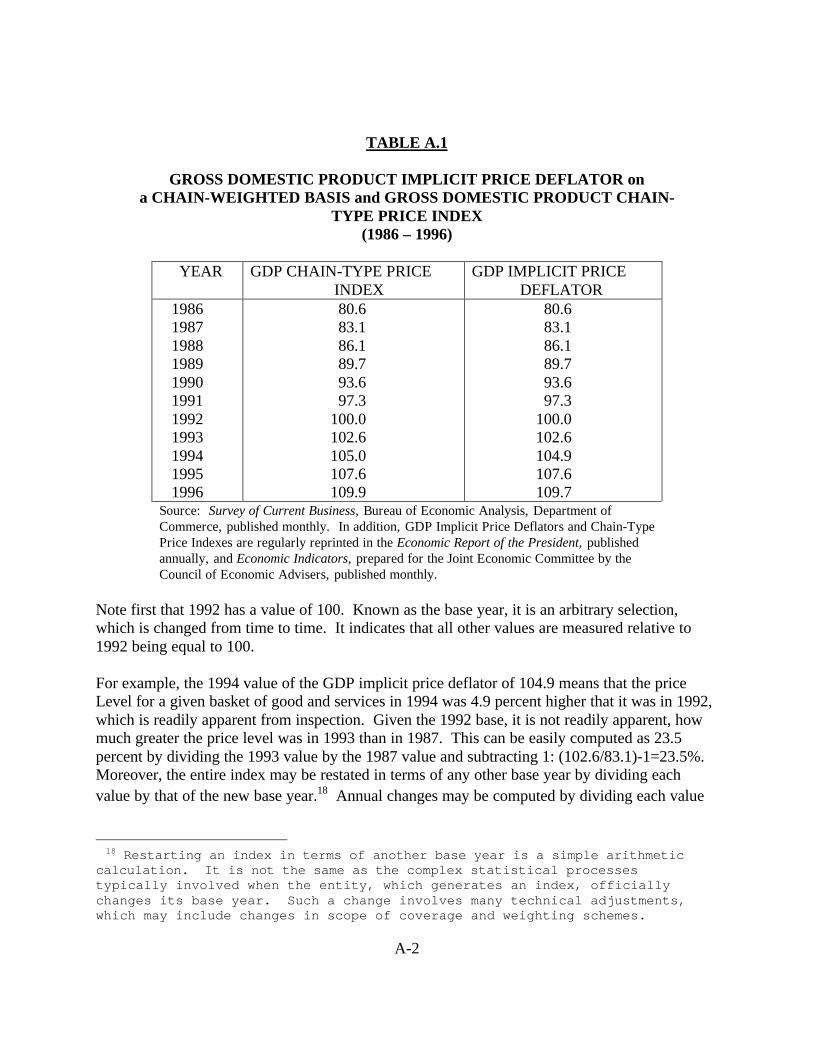
A-2

TABLE A.1

GROSS DOMESTIC PRODUCT IMPLICIT PRICE DEFLATOR ona CHAIN-WEIGHTED BASIS and GROSS DOMESTIC PRODUCT CHAIN-

TYPE PRICE INDEX(1986 – 1996)

YEAR GDP CHAIN-TYPE PRICE INDEX

GDP IMPLICIT PRICE DEFLATOR

1986 1987 1988 1989 1990 1991 1992 1993 1994 1995 1996

80.6 83.1 86.1 89.7 93.6 97.3 100.0 102.6 105.0 107.6 109.9

80.6 83.1 86.1 89.7 93.6 97.3 100.0 102.6 104.9 107.6 109.7

Source: Survey of Current Business, Bureau of Economic Analysis, Department ofCommerce, published monthly. In addition, GDP Implicit Price Deflators and Chain-TypePrice Indexes are regularly reprinted in the Economic Report of the President, publishedannually, and Economic Indicators, prepared for the Joint Economic Committee by theCouncil of Economic Advisers, published monthly.

Note first that 1992 has a value of 100. Known as the base year, it is an arbitrary selection,which is changed from time to time. It indicates that all other values are measured relative to1992 being equal to 100.

For example, the 1994 value of the GDP implicit price deflator of 104.9 means that the priceLevel for a given basket of good and services in 1994 was 4.9 percent higher that it was in 1992,which is readily apparent from inspection. Given the 1992 base, it is not readily apparent, howmuch greater the price level was in 1993 than in 1987. This can be easily computed as 23.5percent by dividing the 1993 value by the 1987 value and subtracting 1: (102.6/83.1)-1=23.5%.Moreover, the entire index may be restated in terms of any other base year by dividing eachvalue by that of the new base year.18 Annual changes may be computed by dividing each value

18 Restarting an index in terms of another base year is a simple arithmeticcalculation. It is not the same as the complex statistical processestypically involved when the entity, which generates an index, officiallychanges its base year. Such a change involves many technical adjustments,which may include changes in scope of coverage and weighting schemes.

A-3

by that of the previous year and subtracting 1. For example, the rate of price change between1995 and 1994 is: (107.6/104/9)-1=2.57%.

To make adjustments for general price level changes requires that the concepts of constantdollars and current dollars be recognized. Current dollar estimates are expressed in the pricelevel of the year in which the resource flows they represent occur. They are the actual amountspent or received. Constant dollar estimates represent the same value as current dollar estimatesbut as measured by the yardstick of the price level of a fixed reference year. Constant dollarscan be specified in terms of any reference year that is desired.

To convert a series expressed in current dollars to constant dollars of a particular year requiresthat all numbers in the series be adjusted for general price level changes. This requires twosteps. First, the general price level index must be transformed so that its base year is the one inwhich the constant dollars are to be stated. As previously noted, this is accomplished by dividingthe general price level index through by its value in the desired base year. The second step is toconvert the specified price series to constant dollars. This requires that it be divided by thevalues produced by step 1. The procedure is illustrated in Table A.2, where the total FAAOperations and Maintenance Budget Appropriation from 1986 through 1996 is converted fromcurrent dollars to 1995 constant dollars. To convert constant dollars to current dollars requiresthat the procedure be reversed. First the deflator series must be divided by its value in the year inwhich the constant dollars are expressed and multiplied by the constant dollar series.

Another conversion likely to be encountered in practice is the transformation of a series from theconstant dollars of one year to those of another. This is accomplished by multiplying theconstant dollar series by the ratio of the price index term for the desired year to the price indexterm for the year in which it is currently expressed, where the base year of the price index isarbitrary. For example, to convert the 1995 constant dollar series in column (4) of Table A.2from 1995 constant dollars to 1990 constant dollars requires that each number in column (4) bemultiplied by 87.0/100 from column (2) or 93.6/107.6 from column (1).

A.2.2 Measuring Price Changes of Specific Goods and Services

A related but distinct situation arises when it is necessary to convert the price of a specific item,which is known in one time period, to what it was in the past or will be in the future. For pastprices, this may be accomplished by using an historical price index defined for the particularclass of item in question. For example, suppose it is known that a particular generic kind ofaircraft was worth $2 million dollars in 1995. A price index defined for this general type ofaircraft allows us to determine -- using the procedures described above in Section A.2.1 -- thatthe price of this aircraft has doubled since 1985. We can then estimate the price of this aircraft in1985 as $1 million. Note that this price adjustment provides no information

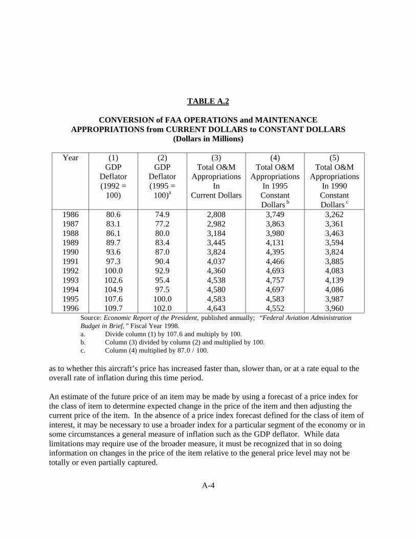
A-4

TABLE A.2

CONVERSION of FAA OPERATIONS and MAINTENANCEAPPROPRIATIONS from CURRENT DOLLARS to CONSTANT DOLLARS

(Dollars in Millions)

Year (1)GDP

Deflator(1992 =

100)

(2)GDP

Deflator(1995 =

100)a

(3)Total O&M

AppropriationsIn

Current Dollars

(4)Total O&M

AppropriationsIn 1995ConstantDollars b

(5)Total O&M

AppropriationsIn 1990ConstantDollars c

19861987198819891990199119921993199419951996

80.683.186.189.793.697.3100.0102.6104.9107.6109.7

74.977.280.083.487.090.492.995.497.5100.0102.0

2,8082,9823,1843,4453,8244,0374,3604,5384,5804,5834,643

3,7493,8633,9804,1314,3954,4664,6934,7574,6974,5834,552

3,2623,3613,4633,5943,8243,8854,0834,1394,0863,9873,960

Source: Economic Report of the President, published annually; “Federal Aviation Administration Budget in Brief,” Fiscal Year 1998.a. Divide column (1) by 107.6 and multiply by 100.b. Column (3) divided by column (2) and multiplied by 100.c. Column (4) multiplied by 87.0 / 100.

as to whether this aircraft’s price has increased faster than, slower than, or at a rate equal to theoverall rate of inflation during this time period.

An estimate of the future price of an item may be made by using a forecast of a price index forthe class of item to determine expected change in the price of the item and then adjusting thecurrent price of the item. In the absence of a price index forecast defined for the class of item ofinterest, it may be necessary to use a broader index for a particular segment of the economy or insome circumstances a general measure of inflation such as the GDP deflator. While datalimitations may require use of the broader measure, it must be recognized that in so doinginformation on changes in the price of the item relative to the general price level may not betotally or even partially captured.

A-5

Estimation of prices of items in the future is typically made for two reasons. The first is forbudget purposes. It is necessary to know how much will actually be spent in the future so that itmay be budgeted for and included in the appropriation process. The second occurs in theconduct of benefit-cost analysis where it is necessary to determine expected benefit or cost valuechanges relative to changes in the general price level. This can be particularly important whendealing with items which are a large component of the analysis and which have price changesthat differ significantly from the overall change in the general price level. Of particularimportance in FAA benefit-cost analysis is the decrease in the cost of electronics relative to thegeneral price level. Suggested methods for dealing with this type of problem are presented inSection A.4.3 below.

A.3 Source of Price Indexes

Numerous different price indexes and forecasts of price indexes are published by governmentaland private organizations. They are available for many narrowly defined commodities andservices, as well as for broader classifications ranging in scope from selected 4-digit SIC19

industries to the overall economy.

Available information and the specific situation should govern the selection of an index for anyparticular price adjustment problem. In general, broadly based measures which reflect the pricesof all goods and services typically purchased by a specific buyer or class of buyer should be usedto make adjustments for inflation -- changes in the general level of prices. Narrowly definedmeasures are appropriate for estimating past or future prices of specific goods or services.Special care should be taken not to use a narrowly defined index to make adjustments for thegeneral level of inflation. For instance, if the objective is to determine the change in the realprice of aircraft over time (as measured relative to other goods and services), it would not beappropriate to deflate an historical time series of aircraft prices by an aircraft price index. Theaircraft price index is built from historical aircraft price changes, and its subsequent applicationto an historical series of aircraft prices would (by definition) give the impression that aircraftprices remained constant. In fact, prices of aircraft may have changed significantly relative toprices of other goods and services in the economy. It would be appropriate to use an indexcomposed of a broad mix of goods and services (such as the implicit GDP deflator), of whichaircraft prices are only a small part, to deflate aircraft prices. On the other hand, if the objectiveis to convert a known aircraft price from an earlier year to a current aircraft price in the studyyear, the use of an aircraft price index would be appropriate. The following section identifiesseveral indexes that may be of use to agency analysts. They are organized by categories relevantto potential FAA economic analyses. These indexes are intended only as suggestions.

19 Industries are classified in the Standard Industrial Classification Manual1987, Office of Management and Budget, 1987. The classification systemoperates in such a way that the definitions become progressively narrowerwith successive additions of numerical digits. The broadest classificationscontain 2 digits and the narrowest 7 digits.

A-6

A.3.1 General Price Level

In January 1996 the Bureau of Economic Analysis, compelled by recent dramatic changes in theU.S. economy’s structure (particularly the spectacular fall in computer prices), adopted a chain-weighted method of computing real GDP and aggregate growth.20 Associated with this newapproach is the GDP Chain-Type Price Index. Both the new GDP Chain-Type Price Index andthe older GDP Implicit Price Deflator represent changes in the prices of all goods an servicesproduced in the United States. Because of their broad coverage, they are widely regarded as thebest single measure of changes in the general price level. Either may be used to adjust timeseries data on current dollar benefits and costs into constant dollars. These measures arecompiled by the Bureau of Economic Analysis on a quarterly and annual basis. Data for themost recent three years are published in the Survey of Current Business.21 Historical data arereprinted in the Economic Indicators.22 Both series are also reprinted annually in the EconomicReport of the President.23

Forecasts for the GDP Implicit Price Deflator and/or GDP Chain-Type Price Index are availablefrom several sources. The Office of Management and Budget provides a projection of the GDPImplicit Price Deflator annually in conjunction with the preparation of the President’s Budget.DRI/McGraw-Hill Data Resources provides forecasts of a wide range of deflators and indexes.The WEFA Group, another full service economic and information consulting firm, also providesa broad range of services including forecasts of deflators and indexes. OMB recommends thatthe GDP deflator projections prepared in conjunction with the President’s Budget be used whenit is necessary to forecast the rate of general inflation and that credible private sector forecasts beused to conduct sensitivity analysis.24

20For a general discussion of the chain-type method, see Charles Steindel,“Chain-Weighting: The New Approach to Measuring GDP”, Current Issues inEconomics and Finance, Vol. 1, Number 9, Federal Reserve Bank of New York,December 1995, pp. 1-5. A more detailed description is given in Mark Lasky,“Forecasting with the New Data”, DRI/McGraw-Hill U.S. Review, February 1996,pp. 38-50, and Mark Lasky “A Preview of the New Chain-Weighted GDP Measures”,DRI/McGraw-Hill U.S. Review, September 1995, pp. 29-37.

21Survey of Current Business, Bureau of Economic Analysis, Department ofCommerce, Washington, D.C., published monthly.

22Economic Indicators, prepared for the Joint Economic Committee by theCouncil of Economic Advisers, U.S. Government Printing Office, Washington,1996, published monthly.

23Economic Report of the President, Council of Economic Advisors, Washington,D.C., published annually in January.

24OMB Circular A-94 (Revised -- October 29, 1992) p. 8.

A-7

A.3.2 Economic Sector Price Levels

Price levels of sectors of the economy represented by the various components of Gross DomesticProduct are measured by either the respective deflator for each component of the respectivechain-weighted index. Component deflators or component chain-weighted indexes likely to beof interest to agency analysts are those for total personal consumption expenditures, fixedinvestment, nonresidential structures, and government purchases of goods and services. Theyare published in the same sources as the GDP Deflator and Chain-Type Price Index. Historicaldata on a chain-weighted basis are available back to 1959. Forecasts of these series are availablefrom the same sources as the GDP Deflator and Chain-Type Price Index. (Section A.3.1).

A.3.3 Construction

Several widely known indexes of construction costs are available in addition to the implicitdeflator. The Boeckh Building Cost Index is compiled monthly by E.H. Boeckh Company,the property division of Mitchell International (internet address:http://www.mitchell.com/boeckh/bcontact.html). It represents construction costs for three typesof buildings: (1) apartments, hotels, and office buildings, (2) commercial and factory buildings,and (3) residential buildings. The Engineering-News Record (ENR) publishes monthly itsConstruction Cost, Common Labor, Skilled Labor, Building Cost and Material Cost (comprisedof cement, steel and lumber) Indexes. These indexes are available separately for 20 U.S. cities.In addition, the ENR uses the Department of Commerce fixed-weighted Construction Cost indexto deflate the value of New Construction Put-In-Place to constant 1992 dollars. On a quarterlybasis, the ENR compiles various construction cost indexes: general-purpose cost, valuation, andspecial purpose indexes. Each December the ENR forecasts these indexes for the next 12months.25

The Federal Highway Administration publishes a quarterly index of highway construction costsin “Price Trends for Federal-Aid Highway Construction.”26 It is based on pricing of sixcomponents of highway construction: common excavation, to indicate the price trend for allroadway excavation; Portland cement concrete pavement and bituminous concrete pavement, toIndicate the price trend for all surfacing types; and reinforcing steel, structural steel, andstructural concrete, to indicate the price trend for structures. 25For detailed description of the index, see “Materials and Labor CostTrends in the U.S.,” Engineering News-Record, (March 9, 1981); pp. 132-137.Also see fourth quarterly Cost Report in ENR for December 23, 1996, andForecast’ 97 in ENR for January 27, 1997.

26“Price Trends for Federal-Aid Highway Construction,” Office ofEngineering, Federal-Aid and Design Division, Federal Highway Administration,publication number FHWA-PD-95-006.

A-8

A.3.4 Energy

As a component of the Producer Price Index (PPI), the Bureau of Labor Statistics compilesmonthly indexes for the prices of coal, coke, gas fuels, electric power, crude petroleum, andrefined petroleum products -- gasoline, kerosene and jet fuels, light fuel oils, residual fuels -- aswell as a composite of them. These are published in the PPI Detailed Report27 or in TheMonthly Labor Review.28 The PPI indexes are also available on the BLS web site athttp://stats.bls.gov.

In addition, the Energy Information Administration of the U.S. Department of Energy publishesthe Annual Energy Review and Annual Energy Outlook. For most series historical energystatistics are given from 1949 through the current year. The Annual Energy Outlook containsprojections to 2015. Most of the data are also available electronically at http:/www/eia.doe.gov.

A.3.5 Electronics and Computers

Also contained in the Producer Price Indexes are several components representing electric andelectronic devices. The broadest category is for electrical machinery and equipment.It represents such items as wiring devices, instruments, motors, transformers, switching gear,electric lamps, and electric components and accessories. An index for each of thesesubcomponents is also available. The electric and electronic devices index is published in theMonthly Labor Review and the subcomponent indexes in the monthly PPI Detailed Report.29 Inaddition, the PPI Detailed Report provides indexes for specific SIC electronics industries—electron tubes (SIC 3671), printed circuit boards (SIC 3672), semiconductors (SIC 3674),electronic capacitors (SIC 3675), electronic resistors (SIC 3676), electronic coils andtransformers (SIC 3677) and electronic connectors (SIC 3578). Computers are aggregated undera broad category -- Office, Computing, and Accounting Machines (SIC 357). At the four-digitlevel, the computer industry is represented in the PPI by electronic computers (SIC 3571),computer storage devices (SIC 3572), computer terminals (SIC 3575), and computer peripheralequipment, n.e.c. (SIC 3578).

27The PPI Detailed Report, Bureau of Labor Statistics, Department f Labor,published monthly.

28The Monthly Labor Review, Bureau of Labor Statistics, Department of Labor,published monthly.

29The PPI Detailed Report, Bureau of Labor Statistics, Department of Labor,published monthly.

A-9

A.3.6 Aircraft and Parts

In addition, BLS publishes the PPI indexes for aircraft and parts. These consist of anaggregate index for aircraft and parts (SIC 372) and more detailed indexes: aircraft (SIC3721), aircraft engine and engine parts (SIC 3724), and aircraft parts auxiliary equipment,n.e.c. (SIC 3728). DRI provides a forecast of these indexes upon customer request.

A.4 Treatment of Inflation in Benefit-Cost Analysis

As a general rule, inflation should not be permitted to affect the outcome of benefit-costanalyses. Such studies are concerned with real quantities -- resources consumed and benefitsprovided. The dollar is used only as the yardstick of value measurement. Because changes inthe unit of measurement cannot affect the relationship between the real quantities, allowingprice changes to affect the analysis will distort the results. This section presents methodologyfor ensuring that inflation does not impact benefit-cost analysis and produce such distortions.

A.4.1 Constant or Nominal Dollars

OMB now permits benefit-cost analyses to be conducted in either nominal or current dollars orin constant dollars of a particular year.30 Effects of inflation are excluded by choosing eithernominal dollars or constant dollars and avoiding mixing-up both in the same analysis and byusing a nominal discount rate if the analysis is conducted in nominal dollars and a real discountrate if the analysis is conducted in constant dollars. (See Chapter 5, 11.C. of "EconomicAnalysis of Investment and Regulatory Decisions -- Revised Guide," FAA-APO-98-4, datedJanuary 1998.) OMB implies a preference for the use of constant dollars unless most of theunderlying values are initially available in nominal dollars. Although some conversions fromnominal to constant or vice-versa may be necessary to get all values into one form or the other,the choice of nominal or constant dollars should be made so as to minimize the conversionsrequired.

Another consideration in selecting nominal or constant dollars is whether or not private sectoroptimizing behavior is endogenous within the analysis to be undertaken. If it is, the analystmust recognize that private sector actions are based on after tax impacts and that taxes aretypically a function of nominal values. (For example, an analysis of alternative policiesdesigned to influence aircraft operations to replace older aircraft with newer, quieter oneswould need to incorporate tax impacts of replacement.) Where the outcome of an analysisdepends significantly on such behavior, the analyst should seriously consider use of nominal

30“OMB Circular A-94” (Revised -- October 29, 1992) p. 8. The previousversion of Circular A-94 (March 27, 1972) p. 3, had required that allanalyses be conducted in constant dollars.

A-10

values when designing the study.Current FAA practice is to conduct benefit-cost analyses inconstant dollars. Although use of nominal values may be advantageous in certain cases, FAAanalyses should continue the use of constant dollars as normal practice unless there is goodreason to do otherwise. The following guidance presumes the use of constant dollars.

A.4.2 Period Between Analysis Date and Project Start Date

The selection of the yardstick of value measurement is arbitrary. The constant dollars of oneyear are as good as the constant dollars of any other year as far as the economics of theanalysis goes. However, for practical considerations it is recommended that the constantdollars of the year of the analysis be selected as the unit of measurement. This procedure is anatural approach because it permits benefits and costs to be valued at their current prices.Moreover, it avoids the need to transform current prices into past or future year dollars and,with respect to future years, the need to forecast inflation. Note that this recommendation isnot a hard and fast rule and should not be followed when other circumstances so indicate.

A.4.3 Inflation During Project Life

During the projected life of the proposed investment of regulation, changes in the general levelof prices should not be allowed to impact the analysis. Benefits and costs are real quantities;they consist of the goods and services provided by a project and the resources consumed inproviding them. Dollars enter the analysis only as the yardstick of value. To allow the unit ofmeasurement to vary would assign different valuation to the same benefits or costs dependingon the variation in the unit of measurement over the project’s lifetime.31 With the typicalinvestment or regulation during times of increasing prices, large costs occurring early in theproject’s life would be assigned less value than benefits stretching out over the years. Thiscould lead to projects being undertaken which are not worthwhile because inflation had beenallowed to increase benefit values relative to cost values. To avoid such distortions, allbenefits and costs associated with an investment or regulation must be measured in the constantdollars of a particular year -- preferably the year of the analysis for reasons noted in SectionA.4.2 of this appendix.

There is an important qualification (not exception) to the general rule of expressing allquantities in the constant dollars of a particular year. Quantities that increase or decrease invalue more or less than the general price level should have their values adjusted by thedifference between changes in their value and the general price level. This must be done to

31 This statement assumes use of a real discount rate such as the OMBspecified 7 percent rate. It would not hold if a nominal discount rate wereused because the inflation premium built into the nominal rate should remove,at least approximately, the impacts of inflation.

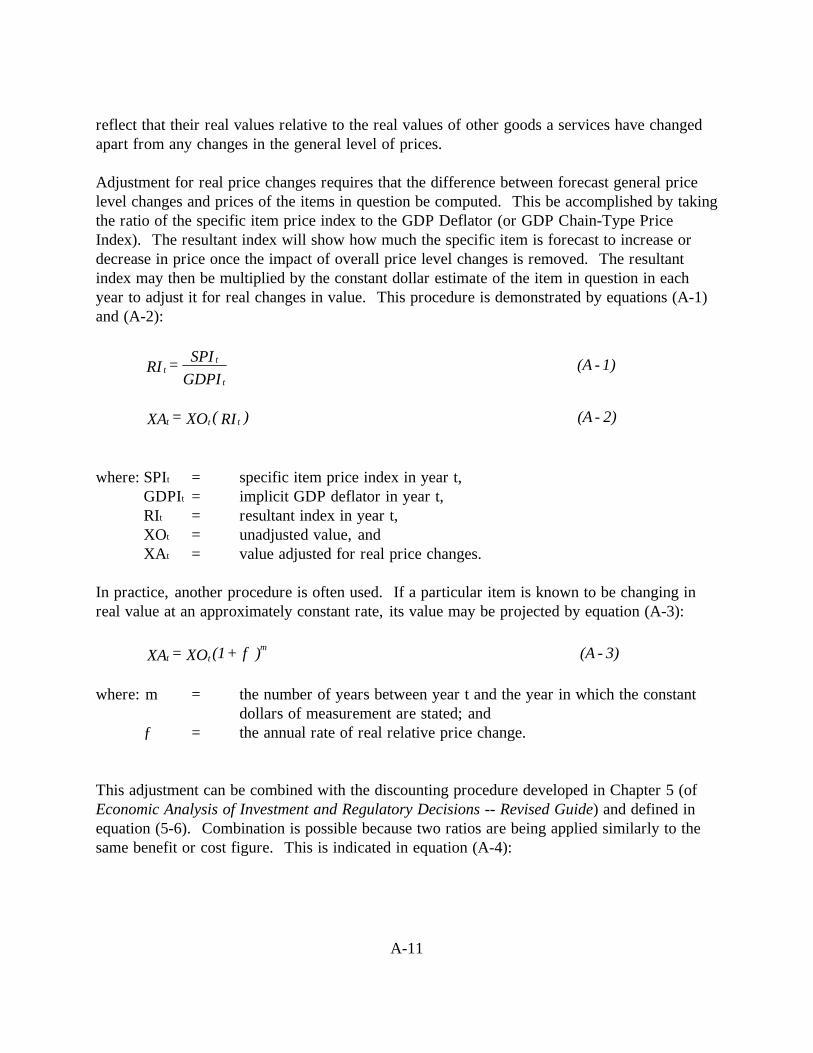
A-11

reflect that their real values relative to the real values of other goods a services have changedapart from any changes in the general level of prices.

Adjustment for real price changes requires that the difference between forecast general pricelevel changes and prices of the items in question be computed. This be accomplished by takingthe ratio of the specific item price index to the GDP Deflator (or GDP Chain-Type PriceIndex). The resultant index will show how much the specific item is forecast to increase ordecrease in price once the impact of overall price level changes is removed. The resultantindex may then be multiplied by the constant dollar estimate of the item in question in eachyear to adjust it for real changes in value. This procedure is demonstrated by equations (A-1)and (A-2):

1)-(A GDPISPI = RI

t

tt

2)-(A )RI(XO = XA ttt

where: SPIt = specific item price index in year t,GDPIt = implicit GDP deflator in year t,RIt = resultant index in year t,XOt = unadjusted value, andXAt = value adjusted for real price changes.

In practice, another procedure is often used. If a particular item is known to be changing inreal value at an approximately constant rate, its value may be projected by equation (A-3):

3)-(A )f+(1XO = XAm

tt

where: m = the number of years between year t and the year in which the constantdollars of measurement are stated; and

ƒ = the annual rate of real relative price change.

This adjustment can be combined with the discounting procedure developed in Chapter 5 (ofEconomic Analysis of Investment and Regulatory Decisions -- Revised Guide) and defined inequation (5-6). Combination is possible because two ratios are being applied similarly to thesame benefit or cost figure. This is indicated in equation (A-4):

A-12

where: Xt = the quantity in year t being adjusted expressed in constant dollarsof the year of initial project implementation,

(B-C)t' = all benefits and costs other than those contained in Xt,r = the discount rate, andk = the total number of periods in the evaluation period of the project

or regulation.

A typical situation where real cost changes must be considered arises with respect toreplacement projects. One advantage of the proposed new system over the old often is that itreplaces an old technology with a new one. In cases where the real cost of the old technologyis projected to increase with time, the absolute amount of the new system’s advantagecontinually increases. While it is proper to include such an ever-increasing advantage in anevaluation, the burden of establishing an appropriate rate of increase rests squarely on theshoulders of the analyst. Conclusions which result solely from assuming large real costincreases in the existing system which are not thoroughly justified are not convincing and areeasily contested.

)4(1

1

)1(

)(

00

−

++

++−

= ∑∑==

Arf

Xr

CBNPV

tk

tt

k

tt

t

B-1

Appendix B: OFFICIAL GUIDANCE ON ECONOMIC ANALYSIS

Official guidance on the need to conduct economic analyses of investment projects andappropriate methodologies for doing so are documented in the following Executive Order andOffice of Management and Budget (OMB) Circular.

B.1 Executive Order 12893 (January 26, 1994): "Principles of Federal InfrastructureInvestment"--Requires Federal agencies to develop and implement plans for infrastructureinvestment and management consistent with the following principles: systematic analysis oftransportation infrastructure project benefits and costs; efficient management of infrastructure;greater private sector participation in infrastructure investment and management; and projectdecisionmaking at the appropriate level of government. The Executive Order requires agenciesto evaluate infrastructure investment at both the program-level (e.g., AIP-level) and individualproject level.

B.2 OMB CIRCULAR A-94 (Revised) (October 29, 1992): "Guidelines and Discount RatesFor Benefit-Cost Analysis of Federal Programs"--Prescribes the methodology to be used inevaluating time-distributed benefits and costs. The circular requires that present values forbenefits and costs of projects such as airport infrastructure projects be calculated using a 7percent real discount rate. It also establishes policy for the treatment of inflation and changes inreal costs. The circular applies to the evaluation of U.S. Government programs and projects.

B.3 Other References: The following references may also prove to be useful.

B.3.1 Methodological:Airport Capacity and Delay, FAA Advisory Circular 150/5060-5, September 9, 1983.

Airport Capacity and Delay, Change 2, December 1, 1995.

Airport Design, FAA Advisory Circular 150/5300-13, September 29, 1989.

Lyon, Randolph M., “Federal Discount Rate Policy, The Shadow Price of Capital, andChallenges for Reforms,” Journal of Environmental Economics and Management, 18, no. 2, part2 (March 1990), S29-S50.

OMB BULLETIN No. 94-16, “Guidance on Executive Order No. 12893, Principles for FederalInfrastructure Investments,” March 7, 1994.

“Policy Guidance Regarding Benefit-Cost Analysis for Airport Capacity Projects RequestingDiscretionary Airport Improvement Program Grant Awards and Letters of Intent,” FederalRegister, Vol. 62, No. 121, June 24, 1997.

“Policy Regarding Revisions of Selection Criteria for Discretionary Airport ImprovementProgram Grant Awards,” Federal Register, Vol. 59, No. 209, October 31, 1994.

B-2

“Policy for Letter of Intent Approvals under the Airport Improvement Program, ” FederalRegister, Vol.59, No. 209, October 31, 1994.

Staffing Standards System—Air Traffic, FAA Order 1380.33B, Federal Aviation Administration,Washington D.C. March 10, 1980.

Staffing Standards System—Airways Facilities Sector Level, FAA Order 1380.40C, FederalAviation Administration, Washington D.C., December, 21, 1992.

Staffing Standards—Regional Logistics Division, FAA Order 1380.42A, Federal AviationAdministration, Washington D.C.

A Study of the High Density Rule, DOT Report to Congress, Department of Transportation,Washington D.C., May 1995.

“Treatment of Value of Life and Injuries in Preparing Economic Evaluations,” Office of theSecretary of Transportation Memorandum January 6, 1993, and subsequent annual updates.

“The Value of Saving Travel Time: Departmental Guidance for Conducting EconomicsEvaluations,” Office of the Secretary of Transportation Memorandum, April 9, 1997.

B.3.2. Data Sources:Air Carrier Traffic Statistics, Bureau of Transportation Statistics, U.S. Department ofTransportation, published monthly.

Economic Indicators, prepared for the Joint Economic Committee by the Council ofEconomic Advisers, U.S. Government Printing Office, Washington D.C., 1996, publishedmonthly.

Economic Report of the President, Council of Economic Advisers, Washington, D.C., publishedannually in January.

FAA Air Traffic Activity, Office of Aviation Policy and Plans, Federal Aviation Administration,Washington D.C., Published annually.

FAA Aviation Forecasts, Office of Aviation Policy and Plans, Federal Aviation Administration,Washington, D.C., published annually.

FAA Statistical Handbook of Aviation, Office of Aviation Policy and Plans, Federal AviationAdministration, Washington D.C., published annually.

“Materials and Labor Cost Trends in the U.S., “Engineering News Record, March 9, 1981, pp.132-137.

B-3

Monthly Labor Review, Bureau of Labor Statistics, Department of Labor, published monthly.

OMB CIRCULAR No. A-76 (Revised Handbook), Performance of Commercial Activities,March 1996.

PPI Detailed Report, Bureau of Labor Statistics, Department of Labor, published monthly.

“Price Trends for Federal-Aid Highway Construction,” publication number FHWA-PD-95-006,Office of Engineering, Federal-Aid and Design Division, Federal Highway Administration,Washington D.C.

Standard Industrial Classification Manual, Office of Management and Budget, 1987.

Standard Abstract of the United States, Department of Commerce, Washington D.C., 1996.

Survey of Current Business, Bureau of Economic Analysis, Department of Commerce,published monthly.

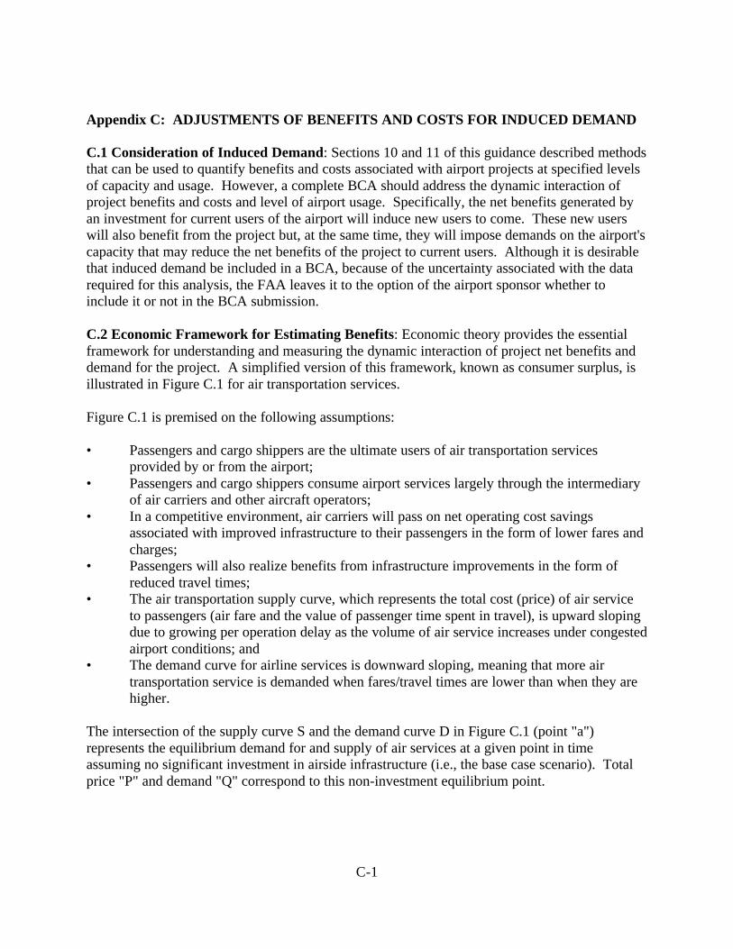
C-1

Appendix C: ADJUSTMENTS OF BENEFITS AND COSTS FOR INDUCED DEMAND

C.1 Consideration of Induced Demand: Sections 10 and 11 of this guidance described methodsthat can be used to quantify benefits and costs associated with airport projects at specified levelsof capacity and usage. However, a complete BCA should address the dynamic interaction ofproject benefits and costs and level of airport usage. Specifically, the net benefits generated byan investment for current users of the airport will induce new users to come. These new userswill also benefit from the project but, at the same time, they will impose demands on the airport'scapacity that may reduce the net benefits of the project to current users. Although it is desirablethat induced demand be included in a BCA, because of the uncertainty associated with the datarequired for this analysis, the FAA leaves it to the option of the airport sponsor whether toinclude it or not in the BCA submission.

C.2 Economic Framework for Estimating Benefits: Economic theory provides the essentialframework for understanding and measuring the dynamic interaction of project net benefits anddemand for the project. A simplified version of this framework, known as consumer surplus, isillustrated in Figure C.1 for air transportation services.

Figure C.1 is premised on the following assumptions:

• Passengers and cargo shippers are the ultimate users of air transportation servicesprovided by or from the airport;

• Passengers and cargo shippers consume airport services largely through the intermediaryof air carriers and other aircraft operators;

• In a competitive environment, air carriers will pass on net operating cost savingsassociated with improved infrastructure to their passengers in the form of lower fares andcharges;

• Passengers will also realize benefits from infrastructure improvements in the form ofreduced travel times;

• The air transportation supply curve, which represents the total cost (price) of air serviceto passengers (air fare and the value of passenger time spent in travel), is upward slopingdue to growing per operation delay as the volume of air service increases under congestedairport conditions; and

• The demand curve for airline services is downward sloping, meaning that more airtransportation service is demanded when fares/travel times are lower than when they arehigher.

The intersection of the supply curve S and the demand curve D in Figure C.1 (point "a")represents the equilibrium demand for and supply of air services at a given point in timeassuming no significant investment in airside infrastructure (i.e., the base case scenario). Totalprice "P" and demand "Q" correspond to this non-investment equilibrium point.

C-2

Price

Passengers

S

S'

D

D

P*

(Fare+

Value of Time)

0

CI

Figure C.1: Consumer Surplus and Role of Induced Demand

P'

P

Q Q*

a

b

d

c

C-3

Now assume that an infrastructure capacity investment would reduce airside congestion andtherefore reduce delay per aircraft operation and passenger. Although traffic demand withrespect to a given total price does not change with the investment (curve D does not shift), theinvestment would permit a higher volume of air service to be provided at the same total price perpassenger, or (alternatively) would allow a lower total price per passenger for the same trafficlevel. This effect is represented by a shift in the air travel supply curve downward, from S to S'.The supply and demand equilibrium is altered from point "a" to point "c", indicating that areduction in the total price of air travel would lead to an increase in demand for air travelservices by passengers.

The net effect of the project is to increase total benefits by an amount equal to the areas C plus I.C is the product of the decrease in total price (P-P*) multiplied by the number of passengers (Q)who would have used the airport even without the investment (pre-existing passengers). Thebenefit to induced or incremental traffic (those passengers who would not have used the airportexcept for the benefits of the investment) is the product of the decrease in total price (P-P*)multiplied by the increase in the number of users (Q*-Q) multiplied by one-half. Multiplicationby one-half is required because the demand curve bisects the area that would be formed by theproduct of (Q-Q*) and (P-P*).32

The consideration of induced demand and consumer surplus is necessary for a correctquantification of benefits.33 Failure to consider induced demand in Figure C.1 would lead theanalyst to conclude that total price per passenger would fall to P' rather than P* and that totalbenefits would equal the rectangle PadP', rather than the polygon PacP* (areas C plus I). In somecases, this error could become severe. Figure C.2 illustrates a case where average delay costs arerising steeply as operations increase at a congested airport. The assumption that

32In economic terms, the adjustment by one-half represents the differencebetween the marginal valuation, read from the demand function, and the newtotal price P* at each quantity above Q.

33Air carriers could also experience a benefit known as producer surplus,provided that air carrier operating expenses are subject to rising marginalcosts. However, this discussion assumes that air carrier operating costs in anuncongested airport environment experience constant returns to scale (i.e., theprice of providing an additional unit of service does not change with thevolume of service). Delay attributable to increases of air service atcongested airports would lead to higher per operation air carrier costs.However, assuming the airport is served by multiple carriers, it is likely thatcarriers will increase service in response to the prevailing average delay peroperation rather than the marginal delay per operation. Under the condition ofa supply curve defined by rising average cost, there would be no producersurplus associated with an expansion of air transportation service.

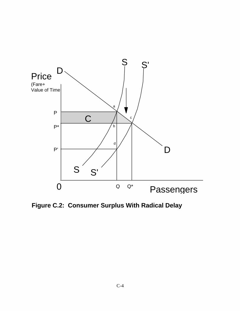
C-4

Price

Passengers

S S'

D

D

(Fare+Value of Time

0

C

Figure C.2: Consumer Surplus With Radical Delay

S S'

Q Q*

P

P'

P*

a

c

b

d

C-5

airport activity would remain unchanged in response to the investment resulting in supply curveS' would lead to an overestimation of future average passenger delay savings equal to thedifference between the area PadP' and PacP*.

C.3 Methodology to Calculate Induced Demand: The guidance for doing simulation analysisof airport capacity projects in Section 10.4.1 recommended that a series of simulations beconducted at passenger demand levels escalating in 2 percent increments from the base casedemand levels simulated. Estimated delay reductions per operation at each demand level shouldthen be recorded in a tabular format (see Table 10.3).

The data in Table 10.3 can be used to determine the impact of the investment on the finaldemand for air transportation services (as measured by the number of passengers). Bycalculating the net impact of delay reductions and other project benefits on passenger trip timeand fare, and by making a reasonable estimate of the total elasticity of demand for air travel atthe study airport, the induced demand scenario in Table 10.3 that best represents an equilibriumdemand/supply solution can be determined. In particular, the scenario with the induced demandlevel (e.g., 2 percent, 4 percent) that most closely conforms to the expected change in demand(passenger response to the actual delay reduction for that scenario as estimated using the totalelasticity of demand) will be the equilibrium scenario. This process is explained in detail in thefollowing subsection.

C.3.1 Total Trip Costs: The first step to reaching an equilibrium demand/supply solution is todetermine the total one-way trip cost for an average passenger currently using the airport. Thiscost consists of two principal components: the average value of one-way passenger transit time(e.g., the time from entering the departure airport to the time of leaving the arrival airport) andthe average one-way ticket fare (which will reflect the cost of providing air service to thatpassenger in a competitive market).

The current total one-way trip cost estimates (time and fare) serve as the basis for evaluating therelative impact of delay reductions and other benefits associated with an investment. Table C.1represents an expansion of the type of data contained in Table 10.3 to include the impact oftravel time and fare associated with a particular investment option in year X. Table C.1 shouldinclude any other quantifiable benefits realized by air travelers, whether or not these benefits arethemselves sensitive to changes in passenger demand. Airlines and passenger service providersare assumed to increase their level of service (subject to constant returns to scale) to meet thechanged demand for air service by passengers.

Table C.1 is presented in a stacked format, but as a spreadsheet would represent a continuoustable extending over 33 columns. For purpose of reference within the table, the columns arelabeled by their alphabetic spreadsheet column headings from A through Z and AA through AG.Five scenarios, representing induced demand levels equal to 0, 2, 4, 6, 8 percent of base casedemand, are identified and developed. Enplanements in the base case are identified in column Cand passengers per enplanement in column D. Total passengers, consisting of base

C-6

TABLE C. 1: CALCULATION OF REDUCED DEMAND

A B C D E F GSCENARIO INDUCED PASSENGER LEVELS

AdditionalPercentageInduced Base Case Induced TotalOver Base Base Case Passengers Demand Demand DemandCase Demand Demand Per (Passengers)(Passengers) (Passengers)

(Explanements) Enplanement (C*D) (B*E) (E*F)

Scenario A 0% 1,000,000 2 2,000,000 0 2,000,000Scenario B 2% 1,000,000 2 2,000,000 40,000 2,040,000Scenario C 4% 1,000,000 2 2,000,000 80,000 2,080,000Scenario D 6% 1,000,000 2 2,000,000 120,000 2,120,000Scenario E 8% 1,000,000 2 2,000,000 160,000 2,160,000

A H I J K L MSCENARIO VALUE OF REDUCED TRIP TIME

Value ofOne-Way Time Time Value of

Base Case Value of Saving of Saving of InvestmentTrip Value of Base Case Investment Investment Case

Time Passenger Trip Time Option Option Trip Time(Minutes) Time ((H/60)*I) (Minutes) ((K/60)*I) (J-L)

Scenario A 150 $26.70 $111.25 2.9 $1.29 $109.96Scenario B 150 $26.70 $111.25 2.7 $1.20 $110.05Scenario C 150 $26.70 $111.25 2.5 $1.11 $110.14Scenario D 150 $26.70 $111.25 2 $0.89 $110.36Scenario E 150 $26.70 $111.25 1.5 $0.67 $110.58

A N O P Q R S T U V W XSCENARIO VALUE OF REDUCED AIR FARE Net

Aircraft Annual Higher Aircraft One-WayOperating Annual Operating Landing Fee Operating Percent Net Trip

One-Way Average Average Cost Financing & Maintenance & O&M Costs Cost Cost Fare FareBase Case Aircraft Passengers Savings Cost Cost From Invest. Savings Savings Savings After

Trip Operating Per Per Pass. From Invest. From Invest, Per Pass. Per Pass. Passed On Per Pass. Invest.Fare Cost/Hour Operation (K/60*O)/P in Year X in Year X ((R+S)/G) (Q-T) To Passenger (U*V) (N-W)

Scenario A $130.00 $1,200.00 50 $1.16 $500,000 $100,000 $0.30 $0.86 100% $0.86 $129.14Scenario B $130.00 $1,200.00 50 $1.08 $500,000 $102,000 $0.30 $0.78 100% $0.78 $129.22Scenario C $130.00 $1,200.00 50 $1.00 $500,000 $104,000 $0.29 $0.71 100% $0.71 $129.29Scenario D $130.00 $1,200.00 50 $0.80 $500,000 $106,000 $0.29 $0.51 100% $0.51 $129.49Scenario E $130.00 $1,200.00 50 $0.60 $500,000 $108,000 $0.28 $0.32 100% $0.32 $129.68

A Y Z AA AB AC AD AE AF AGSCENARIO TOTAL TRIP COST REDUCTION (TIME AND FARE) BEST INDUCED DEMAND ESTIMATE

Total Discrepancy ActualOne-Way One-Way One-Way Percent Estimated Estimated Invest. Case

Base Case Cost Reduction Investment Change in Price Percentage Induced TimeTotal Realized Per Total rip Cost Due Elasticity Induced Relative to Saving PerCost Passenger Cost to Investment of Demand Assumed Closet Operation(N+J) (L+W) (Y-Z) (-Z/Y) Demand (AB*AC) (AD-B) Match (Minutes)

Scenario A $241.25 $2.15 $239.10 -0.89% -1.20 1.07% 1.07%Scenario B $241.25 $1.99 $239.26 -0.82% -1.20 0.99% -1.01% * 2.7Scenario C $241.25 $1.82 $239.43 -0.76% -1.20 0.91% -3.09%Scenario D $241.25 $1.40 $239.85 -0.58% -1.20 0.70% -5.30%Scenario E $241.25 $0.99 $240.26 -0.41% -1.20 0.49% -7.51%

C-7

case (column E) and induced passengers (column F) are summarized in column G. All data inTable C.1 are illustrative and do not reflect an actual airport analysis.

C.3.2 Impact of Time Savings on Trip Time: Column H of Table C.1 reflects the unadjustedaverage passenger one-way trip time in minutes. Passenger trip time can be determined frompassenger and/or operator surveys, consultations with operators, and/or data provided bycommercial data vendors. Estimation of total trip time should make allowances for passengercheck in, transfers to connecting flights, check out, and delay encountered. It is also critical thattrip time be considered for a whole one-way trip, and not simply a segment of a multi-segmentflight. Column I represents the official DOT value of passenger time (see Section 10.5.5.2,FAA-APO-98-8, and APO issued updates to the value of passenger time). Column J is theproduct of columns I and H and represents the time value of the total base case trip. Column Kis the average savings in trip minutes attributable to the investment for different possible levelsof demand (base plus induced demand), taken from column E of Table 10.3. Column Lrepresents the value in passenger time of this delay saving, and M represents the average amountand value of the trip time in column J less the time savings in column L.

C.3.3 Impact of Time Savings on Trip Fare: Column N of Table C.1 is the average trip fare in1996 dollars. Average trip fare can be calculated from the same sources--surveys, consultationswith operators, and/or commercial data vendors--used to determine average trip time. Column Ois the variable operating cost for the average aircraft using the airport (see Section 10.5.5.1).Column P represents the average number of passengers on each flight operation that experiencesthe delay saving noted in column K. Column Q is the value of the delay reduction in terms ofreduced variable aircraft operating costs, calculated by valuing minutes of delay saving fromcolumn K at the aircraft operating cost in column O.

Column Q represents the unadjusted benefit of the investment with regard to its impact onaircraft operating costs on a one-way trip. However, the aircraft operator may or may not passon this saving to passengers in the form of lower trip fares--some will be diverted to the airport(in the form of airport user fees) or may be retained by the carrier itself. In column R of TableC.1, it is assumed that $500,000 in airport user fees must be raised from aircraft operators tocover the project financing cost in year X34. In addition, column S summarizes the annual O&Mcosts in Year X associated with the investment at different levels of demand. Column T showsthe sum of columns R and S, divided by total passengers (column G). In column U, column T(total airport user fees and O&M costs per passenger) is subtracted from column Q (aircraftoperating cost savings per passenger) to yield a net cost savings to the aircraft operator perpassenger. 34In the case of an AIP-funded project, the amount raised through higher ratesand charges to air carriers will be the residual portion of the project notcovered by AIP or payments from airport reserve funds. It should be noted thatairport user fees are considered here because they affect the net gain to theaircraft operator, and thus the average cost savings that may be passed alongto passengers. User fees to cover capital costs are not otherwise consideredin the BCA, however, in that the costs of financing the investment are alreadycaptured in the discounted value of the capital and operating costs of theinvestment (see Section 11).

C-8

In a competitive market, it may be assumed that air carriers will pass along some portion of theirnet cost savings to passengers in the form of lower fares. In column V of Table C.1, it isassumed that aircraft operators pass on 100 percent of these cost savings to their passengers aslower fares (shown in column W).35 Column X represents the one-way base case fare of columnN less the full value of the net per passenger aircraft operating cost savings in column W for eachassumed demand level.

C.3.4 Impact of Change in Total Trip Cost on Final Demand: Columns Y, Z, and AA summarizethe total trip cost before and after the investment for each level of simulated demand, withcolumn Z summing the total time and fare savings realized by each passenger. Column ABrepresents the percentage reduction in total per passenger trip cost attributable to the newinvestment at each of the five simulated demand levels.

C.3.4.1 Total Elasticity of Demand. Column AC introduces the total elasticity of demand for airtravel--a key parameter for determining which of the simulated induced demand levels is thecorrect equilibrium demand level. Total elasticity of demand for air travel is a measure of airtravelers' response to variations in the cost of air travel. This parameter measures the percentagechange in air passenger trips resulting from a one percent change in trip prices. Total elasticitiesare negative because price and quantity demanded are inversely proportional (see Figure C.1).

Total elasticities are highly specific to the characteristics and location of the particular airport(e.g., the carriers serving the airport, local ground access congestion, the proximity of competingairports, and availability of other transportation modes). Estimation of total elasticities specificto an airport may be possible, particularly if carriers at the airport engage in limited fare wars(especially when the fare war is limited to the airport in question). In such cases, changes inairport usage can be measured. Alternatively, surveys of passengers to determine demandresponses must rely on contingent valuation methodologies which are expensive to administerand may yield inaccurate results.

As part of a major study on child restraint systems, FAA sponsored an extensive review of theeconomic literature regarding total elasticity of demand for air travel at a national level. Thefindings of this review are summarized in Chapter 2 and Appendix G of Report to Congress:Child Restraint Systems, Volume 1 and 2, May 1995. The elasticity values found in theacademic literature range from -0.6 to -4.5. Representative values for business and non-businesstravelers are presented in Table C.2. Values in Table C.2 can be tailored to the mix ofpassengers at an airport. Overall weighted values are -0.79 and -1.59 for business and non-business travelers, respectively, with an overall average (assuming the 50/50 mix typical of thenation at large) of -1.2.

35 Technically, (1) 100% of the cost savings should always be passed on in orderto attract new customers and (2) only the marginal customers are the recipientsof the cost savings.

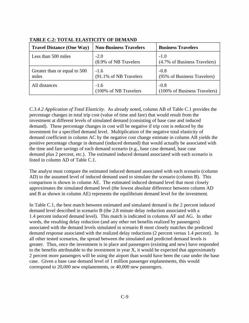
C-9

TABLE C.2: TOTAL ELASTICITY OF DEMAND

Travel Distance (One Way) Non-Business Travelers Business Travelers

Less than 500 miles -2.0(8.9% of NB Travelers

-1.0(4.7% of Business Travelers)

Greater than or equal to 500miles

-1.6(91.1% of NB Travelers

-0.8(95% of Business Travelers)

All distances -1.6(100% of NB Travelers

-0.8(100% of Business Travelers)

C.3.4.2 Application of Total Elasticity. As already noted, column AB of Table C.1 provides thepercentage changes in total trip cost (value of time and fare) that would result from theinvestment at different levels of simulated demand (consisting of base case and induceddemand). These percentage changes in cost will be negative if trip cost is reduced by theinvestment for a specified demand level. Multiplication of the negative total elasticity ofdemand coefficient in column AC by the negative cost change estimate in column AB yields thepositive percentage change in demand (induced demand) that would actually be associated withthe time and fare savings of each demand scenario (e.g., base case demand, base casedemand plus 2 percent, etc.). The estimated induced demand associated with each scenario islisted in column AD of Table C.1.

The analyst must compare the estimated induced demand associated with each scenario (columnAD) to the assumed level of induced demand used to simulate the scenario (column B). Thiscomparison is shown in column AE. The estimated induced demand level that most closelyapproximates the simulated demand level (the lowest absolute difference between column ADand B as shown in column AE) represents the equilibrium demand level for the investment.

In Table C.1, the best match between estimated and simulated demand is the 2 percent induceddemand level described in scenario B (the 2.8 minute delay reduction associated with a1.4 percent induced demand level). This match is indicated in columns AF and AG. In otherwords, the resulting delay reduction (and any other net benefits realized by passengers)associated with the demand levels simulated in scenario B most closely matches the predicteddemand response associated with the realized delay reductions (2 percent versus 1.4 percent). Inall other tested scenarios, the spread between the simulated and predicted demand levels isgreater. Thus, once the investment is in place and passengers (existing and new) have respondedto the benefits attributable to the investment in year X, it would be expected that approximately2 percent more passengers will be using the airport than would have been the case under the basecase. Given a base case demand level of 1 million passenger enplanements, this wouldcorrespond to 20,000 new enplanements, or 40,000 new passengers.

C-10

Although the induced demand effect illustrated in the above example is not large, in some cases(e.g., airports in close regional proximity) total elasticity of demand may be high (4 or above).Given a elasticity coefficient of -6, the induced demand effect in the above example would havebeen 6 percent. Similarly, a project generating major delay savings would also have a magnifiedinduced demand effect.

C.4 Induced Demand at Multiple Forecast Levels: Table C.1 was developed for one point intime, corresponding to that point when demand at the airport would reach 1 millionenplanements under the base case demand forecast. Depending on the expected growth inenplanements under the base case, two or more higher demand levels will have been simulatedfor the investment (see Section 10.4.1), each of which will have its own level of induceddemand. Consequently, Table C.1 should be repeated for each present and future demand levelsimulated.

Travel time and fare estimates for the current period should be adjusted to each of the futureforecast years based on expected growth in delay as measured in the base case scenario. Futuretravel times will be equal to the current travel time plus new delay associated with future traffic.Delay will also increase operator costs by the value of aircraft operating costs associated with thenew delay. This added cost should be converted to a per passenger basis and added to thecurrent average fare to calculate a future base fare for base case (this assumes the cost increase ispassed on to customers).

Because an investment may have greater benefits relative to the base case at higher overalldemand levels, it does not follow that the percentage of induced demand associated with onedemand level (year X) will apply to higher demand levels (year X+10). Thus, induced demandwhich was 3 percent in Table C.1 (associated with 1 million base case enplanements in year X)could be 4 or 6 percent when base case enplanements reach 2 million in year X+20.

C.5 Adjustments of Benefits and Costs to Reflect Induced Demand: Table C.1 was developedto determine the response of users to the airport following the implementation of a new project.Demand response was measured according to the cost savings realized by the ultimate user of thesystem--the passenger. The information contained or developed in the Table C.1 is also criticalto the development of total project benefits and costs, although some further processing isrequired.

C.5.1 Benefits: Benefits from Table C.1 must reflect those to the overall project rather thansimply to passengers. In addition, benefits must be counted differently for pre-existing andinduced passengers.

C.5.1.1 Project Versus Passenger Benefits. Table C.1 measured travel time and fare reductionsrealized by passengers as a means of gauging the change in final demand for airport services thatmay result from an investment. Fare reductions, made possible by lower airline operating costs,were adjusted downward to reflect user charges paid by airlines to the airport sponsor to coverfinancing and O&M costs associated with the investment.

C-11

However, the full cost savings to airlines (whether distributed to the sponsor through usercharges or to the passenger through lower fares or retained by the airline) must be measured asbenefits of the project. In the case of Table C.1, these are measured on a per passenger basis incolumn Q. Project financing and O&M costs are already considered by the BCA process in thetotal capital and O&M cost of the project (adjusted in the discount rate).

C.5.1.2 Benefits To Pre-Existing and Induced Traffic. Benefit information contained inTable C.1 must be interpreted differently for passengers who would have used the airport evenwithout the investment (pre-existing passengers) and those who are induced to use it due to thebenefits of the investment. As noted in Appendix C.1, the benefit to induced passenger traffic isequal to the product of the decrease in price (P-P*) multiplied by the increase in the number ofusers (Q*-Q) multiplied by one-half. From the context of Figure C.1, multiplication by one-halfis required because the demand curve bisects the area that would be formed by the product of (Q-Q*) and (P-P*).

The values in these columns for scenario B would represent the total benefits per pre-existingpassenger, which are summarized in Table C.3. Column B of Table C.3 contains the perpassenger benefits of columns L and Q of Table C.1. These benefits are multiplied by thenumber of pre-existing passengers (column E of Table C.2) to generate total benefits to pre-existing traffic.

Column E of Table C.3 contains the 50 percent factor to scale benefits down by one-half forinduced passengers. The total number of induced passengers for scenario B is listed in column Fof Table C.3. Benefits in column B of Table C.3 are multiplied by the 50 percent factor incolumn E and then by the induced passenger total in column F, yielding total benefits to inducedpassengers in column G. Total benefits for pre-existing and induced passengers are summed incolumn H of Table C.3. An alternate calculation, based solely on the savings per passenger inscenario A of Table C.1 (no induced demand), is provided in column I of Table C.3.

As can be seen when comparing columns G and I of Table C.3, consideration of induced demandleads to an overall reduction in benefits relative to what would have been measured were induceddemand not considered. This result will occur in situations where delay is highly

C-12

TABLE C.3: IMPACT OF INDUCED DEMAND ON BENEFITS

A B C D E F G H I

BENEFIT BASE CASE DEMAND PASSENGERS (PRE-EXISTING)

INDUCED PASSENGERS TOTAL PASSENGERS

Saving forExisting

PassengersPercent

in Year X Pre-Existing Total TotalSaving Due to Passenger Benefits Total Benefit

Per Total Investment Saving Applying Total Induced Benefit W/O CorrectionPre-Existing Pre-Existing (B*C) To Induced Induced Passengers Passengers For Induced

Passenger Passengers Passenger Passengers (B*E) (D+G) Demand

Passenger Time $1.2015 2,000,000 $2,403,000 50% 40,000 $24,030 $2,427,030 $2,581,000Aircraft Operating Cost $1.08 2,000,000 $2,160,000 50% 40,000 $21,600 $2,181,600 $2,320,000Total Benefit $3.2815 2,000,000 $4,563,000 50% 40,000 445,630 $4,608,630 $4,901,000

TABLE C.4: IMPACT OF INDUCED DEMAND ON COSTS

A B

VARIABLE COST

AnnualCost

in Year X

Capital Cost Does not vary with passengervolume

O&M $102,000

C-13

sensitive to increased traffic in both the base and investment cases. Alternatively, in exampleswhere the additional traffic induced by the investment has little or no impact on delay relative tothe base case demand levels (e.g., if the values in column K of Table C.1 did not fall with higherpassenger levels), consideration of induced demand would lead to higher total benefits thanwould be measured were induced demand not considered.

C.5.2 Costs: Relevant cost data found in Table C.1 is associated with O&M expenses listed incolumn S. In this case, O&M is influenced by the amount of traffic using the airport and isassumed to have a constant per passenger value. Thus, O&M totals developed in Section 11 forthe base case are adjusted upwards by the amount of induced passengers associated with scenarioB. O&M costs (adjusted for induced demand) are summarized in Table C.4.

Alternatively, the overall capital costs of the project are not subject to variations in passengerdemand. Financing charges, which reflect the payments needed to pay off loans and bondsissued for project costs not covered by AIP or other grants, are reflected in column R of TableC.1. As noted above, these amounts are considered in Table C.1 only to measure their impact onpassenger demand. The financing cost of project capital, along with the opportunity cost of grantfunds, is captured in the discount rate applied to all project costs and benefits.