F-TODIM: AN APPLICATION OF THE FUZZY TODIM METHOD … · Making, is one of the first Multi-Criteria Decision Making (MCDM) founded on prospect Theory. One of the strong attributes

September 24-28, 2012Rio de Janeiro, Brazil

F-TODIM: AN APPLICATION OF THE FUZZY TODIM METHOD TO RENTAL EVALUATION OF RESIDENTIAL PROPERTIES

Renato A. Krohling Departamento de Engenharia de Produção &

Programa de Pós-graduação em Informática, PPGI

UFES - Universidade Federal do Espírito Santo

Av. Fernando Ferrari, 514, CEP 29075-910

Vitória, Espírito Santo, ES

[email protected]

Talles T. M. de SouzaDepartamento de Informática

UFES - Universidade Federal do Espírito Santo

Av. Fernando Ferrari, 514,CEP 29075-910

Vitória, Espírito Santo, ES

[email protected]

RESUMO

O método de Tomada de Decisão Iterativa Multicritério (TODIM) é um dos primeiros métodos

de tomada decisão baseado na teoria da propensão ao risco. Um característica marcante deste

método é sua capacidade para tratar problemas de tomada de decisão envolvendo riscos.

Contudo, o método TODIM na sua formulação original não é capaz de levar em conta

informações incertas da matriz de decisão. Objetivando atacar esse problema, foi desenvolvido

recentemente pelos autores desse artigo o método Fuzzy TODIM, que é uma extensão do método

TODIM. Dessa forma torna-se possível tratar problemas de tomada de decisão envolvendo riscos

e incertezas. Um estudo de caso ilustrando a aplicação na avaliação de imóveis residenciais para

alugar é apresentado.

Palavras chave. Tomada de decisão multi-critério, teoria da propensão ao risco, fuzzy TODIM

ADM – Apoio à Decisão Multicritério

ABSTRACT

The TODIM method, which is an acronym in Portuguese for Iterative Multi-criteria Decision

Making, is one of the first Multi-Criteria Decision Making (MCDM) founded on prospect

Theory. One of the strong attributes is its capacity to treat risk MCDM problems. Nevertheless,

TODIM in its original formulation is not able to take into account uncertain information of the

decision matrix. In order to tackle this shortcoming, the authors of this paper have recently

developed the Fuzzy TODIM method, which is an extension of TODIM method to handle

uncertain MCDM problems. So, it is possible to handle risk and uncertain MCDM problems. A

case study illustrating the application of the method to rental evaluation of residential properties

is presented.

Keywords. Multi-Criteria Decision Making (MCDM), prospect theory, fuzzy TODIM

MCDM – Multi-criteria Decision Making

431


1. Introduction Complex decision processes may be considered difficult to solve most due to the involved

uncertainties, associated risks and inherent complexities of multi-criteria decision making

(MCDM) problems (Fenton and Wang, 2006). The theory of fuzzy sets and fuzzy logic

developed by Zadeh (1965) has been used to model uncertainty or lack of knowledge and applied

to several MCDM problems. Bellman & Zadeh (1970) introduced the theory of fuzzy sets in

problems of MCDM as an effective approach to treat vagueness, lack of knowledge and

ambiguity inherent in the human decision making process which are known as fuzzy multi-

criteria decision making (FMCDM). See for example Zimmerman (1991) for more information. For real world-problems the decision matrix is affected by uncertainty and may be modeled

using fuzzy numbers. A fuzzy number (Dubois and Prade, 1980) can be seen as an extension of

an interval with varied grade of membership. This means that each value in the interval has

associated a real number that indicates its compatibility with the vague statement associated with

a fuzzy number. So, standard MCDM methods like TOPSIS (Wang and Yoon, 1981) and

PROMETHEE (Brans, Vincke and Marechal, 1986) have been extended using fuzzy numbers

resulting in fuzzy TOPSIS (Wang, Liu, and Zhang, 2005) and fuzzy PROMETHEE (Goumas and

Lygerou, 2000), respectively. Both methods have successfully been applied to solve various

uncertain MCDM problems.

Another important aspect of decision making is that most of the existing MCDM methods are

not able to capture or take into account the risk attitude/preferences of the decision maker in

MCDM. Prospect theory developed by Kahneman and Tversky (1979) is a descriptive model of

individual decision making under condition of risk. Later, Tversky and Kahneman (1992)

developed the cumulative prospect theory, which capture psychological aspects of decision

making under risk. In the prospect theory, the outcomes are expressed by means of gains and

losses from a reference alternative (Salminen, 1994). The value function in prospect theory

assumes an S-shape concave above the reference alternative, which reflects the aversion of risk in

face of gains; and the convex part below the reference alternative reflects the propensity to risk in

case of losses.

As far as we know, one of the first MCDM methods based on prospect theory was proposed by Gomes and Lima (1992). Despite its effectiveness and simplicity in concept, this method

presents some shortcomings because of its inability to deal with uncertainty and imprecision

inherent in the process of decision making. In the original formulation of TODIM (an acronym in

Portuguese for Iterative Multi-criteria Decision Making), the rating of alternatives, which

composes the decision matrix, is represented by crisp values. The TODIM method has many

similarities with the PROMETHEE method, whereas the preference function is replaced by the

prospect function. The TODIM method has been applied to rental evaluation of residential

properties (Gomes and Rangel, 2009) among others applications with good performance.

However, one of the shortcomings of the TODIM method is its inability to handle uncertain

MCDM, which are present in many MCDM problems.

In a previous work (Krohling & de Souza, 2012), we extend the TODIM method by

combining the strong aspects of prospect theory and fuzzy sets to handle uncertain and risk

MCDM and developed the Fuzzy TODIM method, which is able to handle uncertain decision

matrices. In section 2, we provide some background knowledge on fuzzy sets and prospect

theory. In section 3, we present the novel Fuzzy TODIM method, which contains uncertainty in

the decision matrix using trapezoidal fuzzy numbers and the value function of prospect theory to

handle risk attitudes of the decision maker. In section 4, we present a case study to illustrate the

method. In section 5, we present some conclusions and directions for future work.

2. Multi-criteria Decision Making

2.1 Preliminaries on prospect theory The value function used in the prospect theory is described in form of a power law according to

the following expression:

432


if 0( )

( ) if 0

x xv x

x x

α

βθ

≥=

− − < (1)

where α and β are parameters related to gains and losses, respectively. The parameter θ

represents a characteristic of being steeper for losses than for gains. In case of risk

aversion 1.θ > Fig. 1 shows a prospect value function with a concave and convex S-shaped for

gains and losses, respectively. Kahneman and Tversky (1979) experimentally determined the

values of 0.88,and 2.25,α β θ= = = which are consistent with empirical data. Further, they

suggested that the value of θ is between 2.0 and 2.5.

Fig. 1: Value function of prospect theory.

2.2 Preliminaries on fuzzy sets and fuzzy number Next, we provide some basic definitions of fuzzy sets and fuzzy numbers (Wang & Lee, 2009).

Definition 1: A fuzzy set Ã in a universe of discourse X is characterized by a membership

function ( )Ã xµ that assigns each element x in X a real number in the interval [0; 1]. The numeric

value ( )Ã xµ stands for the grade of membership of x in Ã.

Definition 2: A trapezoidal fuzzy number ã is defined by a quadruplet 1 2 3 4( , , , )ã a a a a= as shown

in Fig. 2. The membership function is given by:

1

11 2

2 1

2 3

43 4

4 3

4

0, if

, if

( ) 1, if

, if

0, if

ã

x a

x aa x a

a a

x a x a

a xa x a

a a

x a

µ

<

− ≤ < −

= ≤ ≤ − < ≤

−

>

(2)

Fig. 2: Trapezoidal fuzzy number 1 2 3 4( , , , ).ã a a a a=

433


Definition 2: Let a trapezoidal fuzzy number 1 2 3 4( , , , )ã a a a a= , then the defuzzified value amɶ is

calculated by:

1 2 3 4( )

4ã

a a a am

+ + += ⋅ (3)

Definition 3: Let two trapezoidal fuzzy numbers 1 2 3 4( , , , )ã a a a a= and 1 2 3 4( , , , ),b b b b b=ɶ then the

operation with these fuzzy numbers are defined as follows:

1. Addition of fuzzy numbers (+)

1 2 3 4 1 2 3 4 1 1 2 2 3 3 4 4( ) ( , , , ) ( ) ( , , , ) ( , , , )ã b a a a a b b b b a b a b a b a b+ = + = + + + +ɶ

2. Subtraction of fuzzy numbers (-)

1 2 3 4 1 2 3 4 1 1 2 2 3 3 4 4( ) ( , , , ) ( ) ( , , , ) ( , , , )ã b a a a a b b b b a b a b a b a b− = − = − − − −ɶ

3. Multiplication of fuzzy numbers (x)

1 2 3 4 1 2 3 4 1 1 2 2 3 3 4 4( ) ( , , , ) ( ) ( , , , ) ( , , , )ã x b a a a a x b b b b a b a b a b a b= = ⋅ ⋅ ⋅ ⋅ɶ

4. Division of fuzzy numbers (/)

1 2 3 4 1 2 3 4 1 4 2 3 3 2 4 1(/) ( , , , ) (/) ( , , , ) ( / , / , / , / )ã b a a a a b b b b a b a b a b a b= =ɶ

5. Multiplication by a scalar number k

1 2 3 4 1 2 3 4( , , , ) ( , , , ).kã k a a a a ka ka ka ka= =

Definition 4: Let two trapezoidal fuzzy numbers 1 2 3 4( , , , )ã a a a a= and 1 2 3 4( , , , ),b b b b b=ɶ then the

distance between them (Mahdavi et al., 2008) is calculated by:

42

1 1

1 {1,3}

1( , ) ( ) ( )( ) .

6i i i i i i

i i

d a b b a b a b a+ += ∈

= − + − − ∑ ∑ɶɶ

(4)

Definition 5: Let the trapezoidal fuzzy number 1 2 3 4( , , , ),ã a a a a= then the following properties of

prospect value of fuzzy numbers are given as follows:

1 2 3 4 1 2 3 4

1 2 3 4 1 2 3 4

1 2 3 4 1 1 3 4

1 2 3

(1) if 0, 0, 0, 0, then ( ) [ , , , ]

(2) if 0, 0, 0, 0 then ( ) [ , , , ]

(3) if 0, 0, 0, 0, then ( ) [ , , , ]

(4) if 0, 0, 0,

a a a a v a a a a a

a a a a v a a a a a

a a a a v a a a a a

a a a

α α α α

β β β β

β β α α

≥ ≥ ≥ ≥ =

≤ ≤ ≤ ≤ = −θ −θ −θ −θ

≤ ≤ ≥ ≥ = −θ −θ

≤ ≥ ≥

ɶ

ɶ

ɶ

4 1 2 3 4

1 2 3 4 1 2 3 4

0, then ( ) [ , , , ]

(5) if 0, 0, 0, 0 then ( ) [ , , , ]

with [0,1],

a v a a a a a

a a a a v a a a a a

β α α α

β β β α

≥ = −θ

≤ ≤ ≤ ≥ = −θ −θ −θ

α∈ β∈[0,1],θ >1.

ɶ

ɶ

3 Fuzzy Multicriteria Decision Making

3.1 Description of decision making problem with uncertain decision matrixLet us consider the fuzzy decision matrix A, which consists of alternatives and criteria, described

by:

1

...

m

A

A

A

=ɶɺɺ

1

11 1

1

... n

n

m mn

C C

x x

x x

ɶ ɶ…

⋮ ⋱ ⋮

ɶ ɶ⋯

where 1 2, , , mA A A⋯ are alternatives, 1 2, ,..., nC C C are criteria, ijxɶ are fuzzy numbers that indicates

the rating of the alternative iA with respect to criterion .jC The weight vector

434


( )1 2, ..., nW w w w= composed of the individual weights ( 1,..., )jw j n= for each criterion jC

satisfying 1

1.n

ji

w=

=∑ The data of the decision matrix A come from different sources, so it is

necessary to normalize it in order to transform it into a dimensionless matrix, which allow the

comparison of the various criteria. In this work, we use the normalized decision matrix

with 1,..., , and 1,..., .ij mxnR r i m j n = = =

After normalizing the decision matrix and the weight vector, TODIM begins with the calculation

of the partial dominance matrices and the final dominance matrix. For such calculations the

decision makers need to define firstly a reference criterion, which usually is the criterion with the

highest importance weight. So, rcw indicates the weight of the criterion c divided by the

reference criteria r. TODIM is described in (Gomes and Lima, 1992; Gomes & Rangel, 2009).

The use of numerical values in the rating of alternatives may have limitations to deal with

uncertainties. So, an extension of TODIM is developed to solve problems of decision making

with uncertain data resulting in fuzzy TODIM. In practical applications, the trapezoidal shape of

the membership function is often used to represent fuzzy numbers. Fuzzy models using

trapezoidal fuzzy numbers proved to be very effective for solving decision-making problems

where the available information is imprecise.

The fuzzy TODIM is described in the following.

3.2 The Fuzzy TODIM method The Fuzzy TODIM is described in the following steps:

Step 1: The criteria are normally classified into two types: benefit and cost. The fuzzy-decision

matrix ij mxnA x = ɶ ɶ with 1,..., , and 1, ...,i m j n= = is normalized which results the correspondent

fuzzy-decision matrix .ij mxnR r = ɶ ɶ The fuzzy normalized value ijrɶ is calculated as:

4

4 1

1

4 1

max( ) with =1,2,3,4 for cost criteria

max ( ) min

min( ) with =1,2,3,4 for benefit criteria

max ( ) min

kij ijk

iji ij i ij

kij ijk

iji ij i ij

a ar k

a a

a ar k

a a

−=

−

−=

− (5)

Step 2: Calculate the dominance of each alternative iAɶ over each alternative jAɶ using the

following expression:

1

( , ) ( , ) ( , )m

i j c i jc

A A A A i jδ φ=

= ∀∑ɶ ɶ ɶ ɶ (6)

where

( )

( )

1

( )

1

( )

( , ) if [ ( )] 0

( , ) 0, if [ ( )] 0

-1 ( , ) if [ ( )] 0

rcic jc x xm

rcc

c i j x x

mrcc

ic jc x xrc

wd x x m mic jc

w

A A m mic jc

wd x x m mic jcw

φ

θ

=

=

⋅ − >

= − =

⋅ − <

∑

∑

ɶ ɶ

ɶ ɶ

ɶ ɶ

ɶ ɶ

ɶ ɶ

ɶ ɶ

(7)

435


The term ( , )c i jA Aφ ɶ ɶ represents the contribution of the criterion c to the function ( , )i jA Aδ ɶ ɶ when

comparing the alternative i with alternative j. The parameter θ represents the attenuation factor

of the losses, which can be tuned according to the problem at hand. In Equation (7) ( )xm icɶ and ( )xm jcɶ

stands for the defuzzified values of the fuzzy number icxɶ and jcxɶ , respectively. The term

( , )ic jcd x xɶ ɶ designates the distance between the two fuzzy numbers icxɶ and jcxɶ , as defined in

Equation (4). Three cases can occur in Equation (7): i) if the value ( ) ( )x xm mic jc−ɶ ɶ is positive, it

represents a gain; ii) if the value ( ) ( )x xm mic jc−ɶ ɶ is nil; and iii) if the value ( ) ( )x xm mic jc−ɶ ɶ is

negative, it represents a loss. The final matrix of dominance is obtained by summing up the

partial matrices of dominance for each criterion.

Step 3: Calculate the global value of the alternative i by means of normalizing the final matrix of

dominance according to the following expression:

( , ) min ( , )

max ( , ) min ( , )i

i j i j

i j i j

δ δξ

δ δ

−=

−

∑ ∑∑ ∑ (8)

Ordering the values iξ provides the rank of each alternative. The best alternatives are those that

have higher value iξ .

Next, we present results for a case study.

4. Experimental Results 4.1 Case study - Rental evaluation of residential properties This case study considers the rental evaluation of residential properties in the city Volta Redonda,

RJ, Brazil. The information of the decision matrix, which consists of crisp values, was adopted

from Gomes & Rangel (2009). It is listed in Table 1 and is composed for 15 alternatives and 8

criteria. The weight vector is listed in Table 2. The original formulation of the TODIM presents

limitations since it is not possible to take into account uncertainty into the decision matrix. Our

formulation attempts to overcome these limitations by describing the uncertainty in form of

trapezoidal fuzzy numbers. In our study we investigate the case of symmetric and asymmetric

uncertainty.

Table 1. Decision matrix (Gomes and Rangel, 2009).

Alternatives Criteria

C1 C2 C3 C4 C5 C6 C7 C8

A1 3 290 3 3 1 6 4 0

A2 4 180 2 2 1 4 2 0

A3 3 347 1 2 2 5 1 0

A4 3 124 2 3 2 5 4 0

A5 5 360 3 4 4 9 1 1

A6 2 89 2 3 1 5 1 0

A7 1 85 1 1 1 4 0 1

A8 5 80 2 3 1 6 0 1

A9 2 121 2 3 0 6 0 0

A10 2 120 1 3 1 5 1 0

A11 4 280 2 2 2 7 3 1

A12 1 90 1 1 1 5 2 0

A13 2 160 3 3 2 6 1 1

A14 3 320 3 3 2 8 2 1

A15 4 180 2 4 1 6 1 1

436


4.2 Decision matrix with symmetric uncertainty

To the original decision matrix listed in Table 1 was introduced -10%, -5%, +5%, +10%

uncertainty to build up 1 2 3 4, , , ,a a a a respectively in form of trapezoidal fuzzy number according

to:

1 2 3 40.1 , 0.05 , 0.05 , 0.1 ,a m m a m m a m m a m m= − = − = + = +

where m stands for the mean graded (the original crisp value in the Table 1) of the trapezoidal

fuzzy number. Fig. 3 depicts the case for the cell (1,1) corresponding to alternative A1 with

respect to criterion C1 of the fuzzy decision matrix. The trapezoidal fuzzy decision matrix

generated is listed in Table 3.

Table 2. Assigned weights to criteria (Gomes and Rangel, 2009).

C1 0.25

C2 0.15

C3 0.10

C4 0.20

C5 0.05

C6 0.10

C7 0.05

C8 0.10

Table 3. Fuzzy decision matrix with symmetric uncertainty.


C1 C2 C3 C4

A1 [2.7, 2.85, 3.15, 3.3] [261, 275.5, 304.5, 319] [2.7, 2.85, 3.15, 3.3] [2.7,2.85,3.15,3.3]

A2 [3.6, 3.8, 4.2, 4.4] [162, 171, 189, 198] [1.8, 1.9, 2.1, 2.2] [1.8,1.9,2.1,2.2]

A3 [2.7, 2.85, 3.15, 3.3] [312.3, 329.65, 364.35, 381.7] [0.9, 0.95, 1.05, 1.1] [1.8,1.9,2.1,2.2]

A4 [2.7,2.85, 3.15, 3.3] [111.6, 117.8, 130.2, 136.4] [1.8, 1.9, 2.1, 2.2] [2.7,2.85,3.15,3.3]

A5 [4.5, 4.75, 5.25, 5.5] [324, 342, 378, 396] [2.7, 2.85, 3.15, 3.3] [3.6,3.8,4.2,4.4]

A6 [1.8, 1.9, 2.1, 2.2] [80.1, 84.55, 93.45, 97.9] [1.8, 1.9, 2.1, 2.2] [2.7,2.85,3.15,3.3]

A7 [0.9, 0.95, 1.05, 1.1] [76.5, 80.75, 89.25, 93.5] [0.9, 0.95, 1.05, 1.1] [0.9,0.95,1.05,1.1]

A8 [4.5, 4.75, 5.25, 5.5] [72, 76, 84, 88] [1.8, 1.9, 2.1, 2.2] [2.7,2.85,3.15,3.3]

A9 [1,8, 1.9, 2.1, 2.2] [108.9, 114.95, 127.05, 133.1] [1.8, 1.9, 2.1, 2.2] [2.7,2.85,3.15,3.3]

A10 [1.8, 1.9, 2.1, 2.2] [108, 114, 126, 132] [0.9, 0.95, 1.05, 1.1] [2.7,2.85,3.15,3.3]

A11 [3.6, 3.8, 4.2, 4.4] [252, 266, 294, 308] [1.8, 1.9, 2.1, 2.2] [1.8,1.9,2.1,2.2]

A12 [0.9,0.95, 1.05, 1.1] [81, 85.5, 94.5, 99] [0.9, 0.95, 1.05, 1.1] [0.9,0.95,1.05,1.1]

A13 [1.8, 1.9, 2.1, 2.2] [144,152,168, 176] [2.7, 2.85, 3.15, 3.3] [2.7,2.85,3.15,3.3]

A14 [2.7, 2.85, 3.15, 3.3] [288, 304, 336, 352] [2.7, 2.85, 3.15, 3.3] [2.7,2.85,3.15,3.3]

A15 [3.6, 3.8, 4.2, 4.4] [162, 171, 189, 198] [1.8, 1.9, 2.1, 2.2] [3.6,3.8,4.2,4.4]

437


Table 3. Fuzzy decision matrix with symmetric uncertainty (cont.).

Fig. 3: Symmetric trapezoidal fuzzy number (2.7, 2.85, 3.15, 3.3)ã = .

For comparisons purpose, we first apply the TODIM method to the original crisp matrix listed in

Table 1 in order to get the reference ranking of the alternatives. Since the TODIM and the F-

TODIM use the parameter ,θ we adopt the reference value 1θ = (Gomes & Rangel, 2009). Next,

we apply the F-TODIM method to the fuzzy trapezoidal matrix with symmetric uncertainty given

in Table 3. In order to study the influence of the parameter ,θ we also use the value 2.5θ = as

suggested by Abdellaoui (2000). The ranking of the alternatives is shown in Table 4. In order to

compare the results we adopt those results obtained from Gomes & Rangel (2009) as reference.

We depict the ranking values for 1θ = and 2.5θ = in Fig. 4 and the prospect function in Fig. 5. As

we can notice, the alternative A5 represents the best alternative for both methods. This means that

the alternative A5 even though affected by uncertainty remains the best alternative. The results

for 1θ = and 2.5θ = are almost the same, which indicates the robustness of the method. In

general, the order of the alternatives obtained by F-TODIM compared to TODIM is different.


C5 C6 C7 C8

A1 [0.9, 0.95, 1.05, 1.1] [5.4, 5.7, 6.3, 6.7] [3.6,3.8,4.2,4.4] [0]

A2 [0.9, 0.95, 1.05, 1.1] [3.6,3.8,4.2,4.4] [1.8,1.9,2.1,2.2] [0]

A3 [1.8, 1.9, 2.1, 2.2] [4.5, 4.75, 5.25, 5.5] [0.9,0.95,1.05,1.1] [0]

A4 [1.8, 1.9, 2.1, 2.2] [4.5, 4.75, 5.25, 5.5] [3.6,3.8,4.2,4.4] [0]

A5 [3.6, 3.8, 4.2, 4.4] [8.1, 8.55, 9.45, 9.9] [0.9,0.95,1.05,1.1] [0.9, 0.95, 1.05, 1.1]

A6 [0.9, 0.95, 1.05, 1.1] [4.5, 4.75, 5.25, 5.5] [0.9,0.95,1.05,1.1] [0]

A7 [0.9, 0.95, 1.05, 1.1] [3.6, 3.8, 4.2, 4.4] [0] [0.9, 0.95, 1.05, 1.1]

A8 [0.9, 0.95, 1.05, 1.1] [5.4, 5.7, 6.3, 6.7] [0] [0.9, 0.95, 1.05, 1.1]

A9 [0] [5.4, 5.7, 6.3, 6.7] [0] [0]

A10 [0.9, 0.95, 1.05, 1.1] [4.5, 4.75, 5.25, 5.5] [0.9,0.95,1.05,1.1] [0]

A11 [1.8, 1.9, 2.1, 2.2] [6.3, 6.65, 7.35, 7.7] [2.7,2.85,3.15,3.3] [0.9, 0.95, 1.05, 1.1]

A12 [0.9, 0.95, 1.05, 1.1] [4.5, 4.75, 5.25, 5.5] [1.8,1.9,2.1,2.2] [0]

A13 [1.8, 1.9, 2.1, 2.2] [5.4, 5.7, 6.3, 6.7] [0.9,0.95,1.05,1.1] [0.9, 0.95, 1.05, 1.1]

A14 [1.8, 1.9, 2.1, 2.2] [7.2, 7.6, 8.4, 8.8] [1.8,1.9,2.1,2.2] [0.9, 0.95, 1.05, 1.1]

A15 [0.9, 0.95, 1.05, 1.1] [5.4, 5.7, 6.3, 6.7] [0.9,0.95,1.05,1.1] [0.9, 0.95, 1.05, 1.1]

438


Table 4. Ranking of the alternatives.

Classification TODIM

crisp

Fuzzy TODIM

a) symmetric 1θ =

Fuzzy TODIM

b) symmetric 2.5θ =

1 A5 A5 A5

2 A14 A14 A14

3 A11 A11 A11

4 A13 A13 A13

5 A1 A15 A15

6 A15 A1 A1

7 A4 A4 A4

8 A8 A8 A8

9 A3 A2 A3

10 A2 A3 A2

11 A6 A6 A6

12 A10 A10 A10

13 A12 A9 A9

14 A9 A12 A12

15 A7 A7 A7

Fig. 4: Ranking of the alternatives for fuzzy trapezoidal matrix with 10% uncertainty around the mean.

439


Fig. 5: Prospect function for trapezoidal fuzzy matrix with 10% symmetric uncertainty around the

mean.

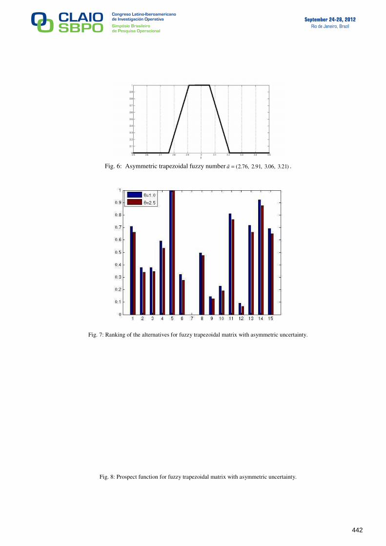
4.3 Decision matrix with asymmetric uncertainty To the original decision matrix listed in Table 1 was introduced -8%, -3%, +2%, +7% uncertainty

to build up 1 2 3 4, , , ,a a a a respectively in form of trapezoidal fuzzy number according to:

1 2 3 40.08 , 0.03 , 0.02 , 0.07a m m a m m a m m a m m= − = − = + = +

where m stands for the mean graded (the original crisp value in the Table 1) of the trapezoidal

fuzzy number. Fig. 6 depicts the case for the cell (1,1) corresponding to alternative A1 with

respect to criterion C1 of the fuzzy decision matrix. The trapezoidal fuzzy decision matrix

generated is listed in Table 5.

Similar to the previous case, we apply the F-TODIM method to the fuzzy trapezoidal matrix with

asymmetric uncertainty given in Table 5.The ranking is shown in Table 6. We depict the ranking

values for 1θ = and 2.5θ = in Fig. 7 and the prospect function in Fig. 8.

Table 5. Fuzzy decision matrix with asymmetric uncertainty.


C1 C2 C3 C4

A1 [2.76, 2.91, 3.06, 3.21] [266.8, 281.3, 295.8, 310.3] [2.76, 2.91, 3.06, 3.21] [2.76, 2.91, 3.06, 3.21]

A2 [3.68, 3.88, 4.08, 4.28] [165.6, 174.6, 183.6, 192.6] [1.84, 1.94, 2.04, 2.14] [1.84, 1.94, 2.04, 2.14]

A3 [2.76, 2.91, 3.06, 3.21] [319.24, 336.59, 353.94, 371.29] [0.92, 0.97, 1.02, 1.07] [1.84, 1.94, 2.04, 2.14]

A4 [2.76, 2.91, 3.06, 3.21] [114.08, 120.28, 126.48, 132.68] [1.84, 1.94, 2.04, 2.14] [2.76, 2.91, 3.06, 3.21]

A5 [4.6, 4.85, 5.1, 5.35] [331.2, 349.2, 367.2, 385.2] [2.76, 2.91, 3.06, 3.21] [3.68, 3.88, 4.08, 4.28]

A6 [1.84, 1.94, 2.04, 2.14] [81.88, 86.33, 90.78, 95.23] [1.84, 1.94, 2.04, 2.14] [2.76, 2.91, 3.06, 3.21]

A7 [0.92, 0.97, 1.02, 1.07] [78.2, 82.45, 86.7, 90.95] [0.92, 0.97, 1.02, 1.07] [0.92, 0.97, 1.02, 1.07]

A8 [4.6, 4.85, 5.1, 5.35] [73.6, 77.6, 81.6, 85.6] [1.84, 1.94, 2.04, 2.14] [2.76, 2.91, 3.06, 3.21]

A9 [1.84, 1.94, 2.04, 2.14] [111.32, 117.37, 123.42, 129.47] [1.84, 1.94, 2.04, 2.14] [2.76, 2.91, 3.06, 3.21]

A10 [1.84, 1.94, 2.04, 2.14] [110.4, 116.4, 122.4, 128.4] [0.92, 0.97, 1.02, 1.07] [2.76, 2.91, 3.06, 3.21]

A11 [3.68, 3.88, 4.08, 4.28] [257.6, 271.6, 285.6, 299.6] [1.84, 1.94, 2.04, 2.14] [1.84, 1.94, 2.04, 2.14]

A12 [0.92, 0.97, 1.02, 1.07] [82.8, 87.3, 91.8, 96.3] [0.24, 0.32, 1.39, 1.74] [0.92, 0.97, 1.02, 1.07]

A13 [1.84, 1.94, 2.04, 2.14] [147.2, 155.2, 163.2, 171.2] [0.92, 0.97, 1.02, 1.07] [2.76, 2.91, 3.06, 3.21]

A14 [2.76, 2.91, 3.06, 3.21] [294.4, 310.4, 326.4, 342.4] [0.92, 0.97, 1.02, 1.07] [2.76, 2.91, 3.06, 3.21]

A15 [3.68, 3.88, 4.08, 4.28] [165.6, 174.6, 183.6, 192.6] [1.84, 1.94, 2.04, 2.14] [3.68, 3.88, 4.08, 4.28]

440


Table 5. Fuzzy decision matrix with asymmetric uncertainty (cont.).

As we can notice, the alternative A5 represents the best alternative for both methods.

This means that the alternative A5 even though affected by uncertainty continues to be the better

alternative. For 1θ = and 2.5θ = the order of the alternatives is almost the same. In general, the

order of the alternatives obtained by F-TODIM compared to TODIM is different.

Table 6. Ranking of alternatives.

Classification TODIM

crisp

Fuzzy TODIM

b) asymmetric 1θ =

Fuzzy TODIM

b) asymmetric 2.5θ =

1 A5 A5 A5

2 A14 A14 A14

3 A11 A11 A11

4 A13 A13 A13

5 A1 A15 A15

6 A15 A1 A1

7 A4 A4 A4

8 A8 A8 A8

9 A3 A2 A3

10 A2 A3 A2

11 A6 A6 A6

12 A10 A10 A10

13 A12 A9 A9

14 A9 A12 A12

15 A7 A7 A7


C5 C6 C7 C8

A1 [0.92, 0.97, 1.02, 1.37] [5.52, 5.82, 6.12, 6.42] [3.68, 3.88, 4.02 4.28] [0]

A2 [0.92, 0.97, 1.02, 1.37] [3.68, 3.88, 4.08, 4.28] [1.84, 1.94, 2.04, 2.14] [0]

A3 [1.84, 1.94, 2.04, 2.14] [4.6, 4.85, 5.1, 5.35] [0.92, 0.97, 1.02, 1.07] [0]

A4 [1.84, 1.94, 2.04, 2.14] [4.6, 4.85, 5.1, 5.35] [3.68, 3.88, 4.02 4.28] [0]

A5 [3.68, 3.88, 4.08, 4.28] [8.28, 8.73, 9.18, 9.63] [0.92, 0.97, 1.02, 1.07] [0.92, 0.97, 1.02, 1.07]

A6 [0.92, 0.97, 1.02, 1.37] [4.6, 4.85, 5.1, 5.35] [0.92, 0.97, 1.02, 1.07] [0]

A7 [0.92, 0.97, 1.02, 1.37] [3.68, 3.88, 4.08, 4.28] [0] [0.92, 0.97, 1.02, 1.07]

A8 [0.92, 0.97, 1.02, 1.37] [5.52, 5.82, 6.12, 6.42] [0] [0.92, 0.97, 1.02, 1.07]

A9 [0] [5.52, 5.82, 6.12, 6.42] [0] [0]

A10 [0.92, 0.97, 1.02, 1.37] [4.6, 4.85, 5.1, 5.35] [0.92, 0.97, 1.02, 1.07] [0]

A11 [1.84, 1.94, 2.04, 2.14] [6.44, 6.79, 7.14, 7.49] [2.76, 2.91, 3.06, 3.21] [0.92, 0.97, 1.02, 1.07]

A12 [0.92, 0.97, 1.02, 1.37] [4.6, 4.85, 5.1, 5.35] [1.84, 1.94, 2.04, 2.14] [0]

A13 [1.84, 1.94, 2.04, 2.14] [5.52, 5.82, 6.12, 6.42] [0.92, 0.97, 1.02, 1.07] [0.92, 0.97, 1.02, 1.07]

A14 [1.84, 1.94, 2.04, 2.14] [7.36, 7.76, 8.16, 8.56] [1.84, 1.94, 2.04, 2.14] [0.92, 0.97, 1.02, 1.07]

A15 [0.92, 0.97, 1.02, 1.37] [5.52, 5.82, 6.12, 6.42] [0.92, 0.97, 1.02, 1.07] [0.92, 0.97, 1.02, 1.07]

441


Fig. 6: Asymmetric trapezoidal fuzzy number (2.76, 2.91, 3.06, 3.21)ã = .

Fig. 7: Ranking of the alternatives for fuzzy trapezoidal matrix with asymmetric uncertainty.

Fig. 8: Prospect function for fuzzy trapezoidal matrix with asymmetric uncertainty.

442


5. Conclusions In this work, we have applied the fuzzy TODIM method, for short, F-TODIM for multi-criteria

decision making to tackle problems affected by uncertainty. The F-TODIM has been investigated

for a case study consisting of rental evaluation of residential properties where the decision matrix

is represented by trapezoidal fuzzy numbers. In general, the order of the alternatives obtained by

F-TODIM compared to TODIM is different since F-TODIM is a more general approach taking

into account uncertainty. The standard TODIM, in its original formulation, is only applicable to

crisp decision matrices. The F-TODIM method can be applied to more challenging MCDM

problems considering uncertain environments. We currently are expanding the method to other

applications.

References Abdellaoui, M. (2000). Parameter-free elicitation of utility and probability weighting functions.

Management Science, 46, 1497–1512.

Bellman, R.E., & Zadeh, L.A. (1970). Decision-making in a fuzzy environment. Management Science, 17, 141–164.

Brans, J.P., Vincke, P., & Mareschal, B. (1986). How to select and how to rank projects: The

Promethee method. European Journal of Operational Research, 24(2), 228-238. Dubois, D., & Prade, H. Fuzzy Sets and Systems: Theory and Applications. New York:

Academic Press, 1980.

Fenton, N., & Wang, W. (2006). Risk and confidence analysis for fuzzy multicriteria decision

making Knowledge-Based Systems, 19(6), 430-437.

Gomes, L.F.A.M., & Lima, M.M.P.P. (1992). TODIM: Basics and application to multicriteria

ranking of projects with environmental impacts. Foundations of Computing and Decision Sciences, 16 (4), 113–127.

Gomes, L.F.A.M., & Rangel, L.A.D. (2009). An application of the TODIM method to the

multicriteria rental evaluation of residential properties. European Journal of Operational Research 193, 204–211.

Goumas, M. & Lygerou, V. (2000). An extension of the PROMETHEE method for decision

making in fuzzy environment: Ranking of alternative energy exploitation projects. European Journal of Operational Research, 123(3), 606-613.

Hwang, C.L., & Yoon, K.P. Multiple attributes decision making methods and applications.

Berlin: Springer-Verlag, 1981.

Kahneman, D., & Tversky, A. (1979). Prospect theory: An analysis of decision under risk.

Econometrica, 47, 263–292.

Krohling, R.A., & de Souza, T.T.M. (2012). Combining prospect theory and fuzzy numbers to

multi-criteria decision making, Expert Systems with Applications, 39, 11487-11493.

Mahdavi, I., Mahdavi-Amiri, N., Heidarzade, A., & Nourifar, R. (2008). Designing a model

of fuzzy TOPSIS in multiple criteria decision making. Applied Mathematics and Computation,

206(2), 607-617.

Salminen, P. (1994). Solving the discrete multiple criteria problem using linear prospect theory.

European Journal of Operational Research, 72(1), 146–54.

Tversky A., & Kahneman D. (1992). Advances in prospect theory: cumulative representation of

uncertainty. Journal of Risk and Uncertainty, 5(4), 297–323.

Wang, J., Liu, S.Y., & Zhang, J. (2005). An extension of TOPSIS for fuzzy MCDM based on

vague set theory. Journal of Systems Science and Systems Engineering, 14, 73-84. Wang, T.-C. and Lee, H.-D. (2009). Developing a fuzzy TOPSIS approach based on subjective

weights and objective weights. Expert Systems with Applications, 36, 8980-8985.

Zadeh, L.A. (1965). Fuzzy sets. Information and Control, 8, 338-353.

Zimmermann, H. J. Fuzzy set theory and its application. Boston: Kluwer Academic Publishers,

1991.

443

Documents

F-TODIM: AN APPLICATION OF THE FUZZY TODIM METHOD … · Making, is one of the first Multi-Criteria Decision Making (MCDM) founded on prospect Theory. One of the strong attributes