Embed Size (px)
Citation preview

NASA Contractor Report 198248
F-18 High Alpha Research Vehicle (HARV)Parameter Identification Flight Test Maneuversfor Optimal Input Design Validation andLateral Control Effectiveness
E.A. Morelli
Lockheed Martin Engineering and Sciences Co.NASA Langley Research CenterHampton, Virginia
Contract NAS1-19000
December 1995
National Aeronautics and Space AdministrationLangley Research CenterHampton, Virginia 23681-0001
https://ntrs.nasa.gov/search.jsp?R=19960012190 2018-09-01T06:35:39+00:00Z
i
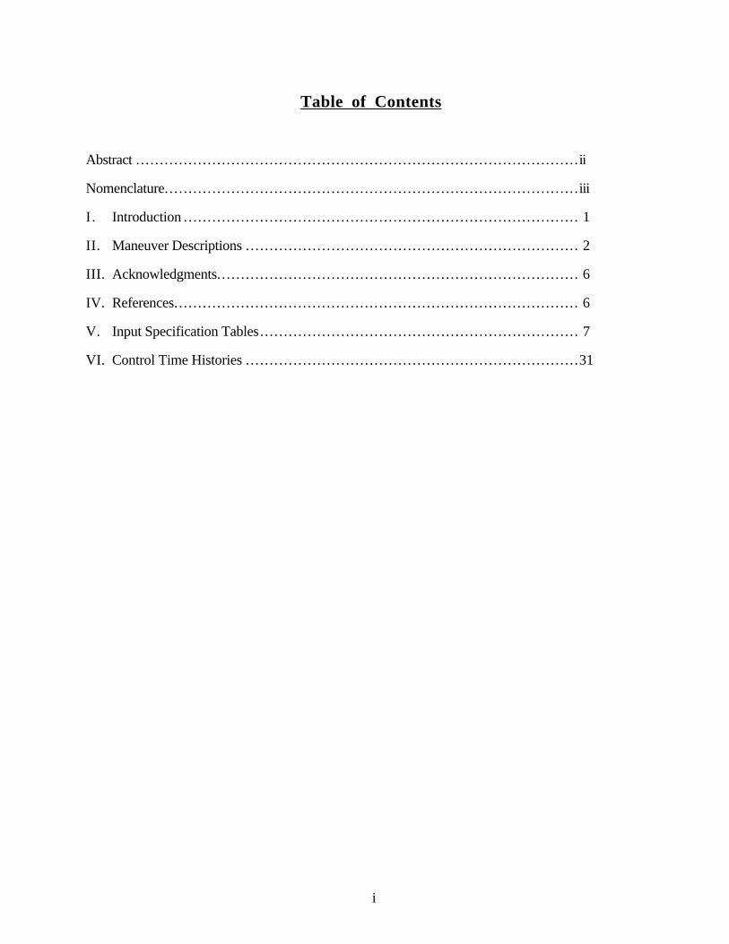
Table of Contents
Abstract . . . . . . . . . . . . . . . . . . . . . . . . . . . . . . . . . . . . . . . . . . . . . . . . . . . . . . . . . . . . . . . . . . . . . . . . . . . . . . . . . . . . . . . . . . . . . ii
Nomenclature.. . . . . . . . . . . . . . . . . . . . . . . . . . . . . . . . . . . . . . . . . . . . . . . . . . . . . . . . . . . . . . . . . . . . . . . . . . . . . . . . . . . . . . iii
I . Introduction .. . . . . . . . . . . . . . . . . . . . . . . . . . . . . . . . . . . . . . . . . . . . . . . . . . . . . . . . . . . . . . . . . . . . . . . . . . . . . . . . . . 1
II. Maneuver Descriptions .. . . . . . . . . . . . . . . . . . . . . . . . . . . . . . . . . . . . . . . . . . . . . . . . . . . . . . . . . . . . . . . . . . . . . 2
III. Acknowledgments.. . . . . . . . . . . . . . . . . . . . . . . . . . . . . . . . . . . . . . . . . . . . . . . . . . . . . . . . . . . . . . . . . . . . . . . . . . . 6
IV. References.. . . . . . . . . . . . . . . . . . . . . . . . . . . . . . . . . . . . . . . . . . . . . . . . . . . . . . . . . . . . . . . . . . . . . . . . . . . . . . . . . . . . 6
V. Input Specification Tables.. . . . . . . . . . . . . . . . . . . . . . . . . . . . . . . . . . . . . . . . . . . . . . . . . . . . . . . . . . . . . . . . . . 7
VI. Control Time Histories .. . . . . . . . . . . . . . . . . . . . . . . . . . . . . . . . . . . . . . . . . . . . . . . . . . . . . . . . . . . . . . . . . . . . .31

ii
Abstract
Flight test maneuvers are specified for the F-18 High Alpha Research Vehicle (HARV). Themaneuvers were designed for open loop parameter identification purposes, specifically for optimalinput design validation at 5 degrees angle of attack, identification of individual strake effectiveness at40 and 50 degrees angle of attack, and study of lateral dynamics and lateral control effectiveness at 40and 50 degrees angle of attack. Each maneuver is to be realized by applying square wave inputs tospecific control effectors using the On-Board Excitation System (OBES). Maneuver descriptions andcomplete specifications of the time / amplitude points defining each input are included, along withplots of the input time histories.
iii
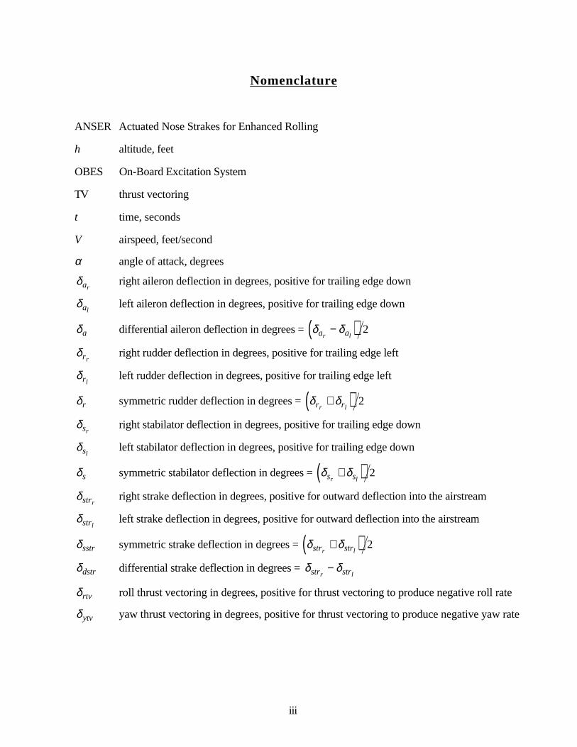
Nomenclature
ANSER Actuated Nose Strakes for Enhanced Rolling
h altitude, feet
OBES On-Board Excitation System
TV thrust vectoring
t time, seconds
V airspeed, feet/second
α angle of attack, degrees
δarright aileron deflection in degrees, positive for trailing edge down
δalleft aileron deflection in degrees, positive for trailing edge down
δa differential aileron deflection in degrees = δar− δal( ) 2
δrrright rudder deflection in degrees, positive for trailing edge left
δrlleft rudder deflection in degrees, positive for trailing edge left
δr symmetric rudder deflection in degrees = δrr+ δrl( ) 2
δsrright stabilator deflection in degrees, positive for trailing edge down
δslleft stabilator deflection in degrees, positive for trailing edge down
δs symmetric stabilator deflection in degrees = δsr+ δsl( ) 2
δstrrright strake deflection in degrees, positive for outward deflection into the airstream
δstrlleft strake deflection in degrees, positive for outward deflection into the airstream
δsstr symmetric strake deflection in degrees = δstrr+ δstrl( ) 2
δdstr differential strake deflection in degrees = δstrr− δstrl
δrtv roll thrust vectoring in degrees, positive for thrust vectoring to produce negative roll rate
δ ytv yaw thrust vectoring in degrees, positive for thrust vectoring to produce negative yaw rate

iv
subscripts
o nominal or trim value

5
I. Introduction
The F-18 High Alpha Research Vehicle (HARV) is a highly instrumented research aircraft usedin the NASA High Alpha Technology Program1. Objectives for this program include investigatingadvanced flight testing techniques and determining the effectiveness of novel control effectors formaneuvering flight at high angles of attack.
In this work, the technique described in references [2] and [3] was used to design flight testmaneuvers consisting of optimal open loop square wave inputs. These square wave inputs are to beapplied directly to the relevant control effectors by the On-Board Excitation System (OBES)4. Theoptimal input design technique uses dynamic programming to compute globally optimal square waveinputs for model parameter estimation experiments, based on a priori dynamic models. Linear apriori dynamic models were obtained from an F-18 HARV nonlinear simulation5 using central finitedifferences. The maneuvers were designed specifically to collect flight data with maximuminformation content for dynamic modeling purposes.
Specific objectives addressed by the maneuvers specified in this document are:
1. Study the efficacy of optimal square wave inputs implemented by the On-Board ExcitationSystem (OBES) for aircraft parameter identification, including comparison with standard3-2-1-1 input forms. Comparison of piloted optimal square wave inputs with piloteddoublet inputs has been documented in reference [6].
2. Determine individual strake effectiveness at 40 and 50 degrees angle of attack forcomparison with wind tunnel data and results from alternative flight test methods.
3. Study aircraft lateral dynamic response, differential strake effectiveness, and yaw / rollthrust vectoring effectiveness at 40 and 50 degrees angle of attack.
4. Update and verify existing aerodynamic models.
The purpose of this report is to document the specifications for the maneuvers designed toachieve the above objectives.

6
II. Maneuver Descriptions
There are thirteen (13) optimal square wave input maneuvers described in this report. Themaneuvers can be divided into three groups:
1. Five (5) maneuvers for optimal input design validation using the OBES system.
2. Two (2) maneuvers for investigating individual strake effectiveness at 40 and 50 degreesangle of attack using the OBES system.
3. Six (6) maneuvers for studying lateral dynamic response and control effectiveness at 40and 50 degrees angle of attack using the OBES system.
All maneuvers are to be flown using the Actuated Nose Strakes for Enhanced Rolling (ANSER)control law in thrust vectoring (TV) mode7,8. Control definitions and sign conventions are givenabove in the Nomenclature section. Detailed descriptions of the maneuvers in each group appearbelow, with numbering corresponding to that given above.
1. This group of five maneuvers is for studying the optimal input design technique. Initial flightcondition is trim angle of attack 5 degrees and approximately 25,000 feet altitude, with the ANSERcontrol law in TV mode. This initial flight condition applies for all five maneuvers.
The first two maneuvers involve deflection of the symmetric stabilator for studying optimal inputdesign and for longitudinal model updates and verification. The first input is a standard 3-2-1-1input, which will be compared to the second input, an optimal square wave, in terms of efficacy forlongitudinal dynamic response flight testing. It is therefore important that these two maneuvers berun in sequence on the same flight to minimize extraneous influences on the comparison. Inputspecifications for the symmetric stabilator 3-2-1-1 input are given in Table 1, and the optimalsymmetric stabilator specifications are given in Table 2. Figures 1 and 2 show time histories for the3-2-1-1 and optimal inputs, respectively. Both inputs included a rate limit of 40 degrees/second forthe symmetric stabilator.
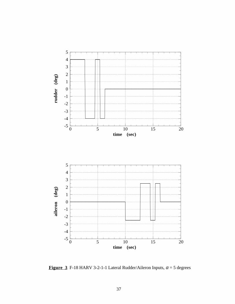
The next three maneuvers involve deflection of the rudder and aileron for studying optimalmultiple input design and for lateral model updates and verification. The first input is a standard3-2-1-1 input, which will be compared to the next two inputs, a sequential optimal square wave and asimultaneous optimal square wave, in terms of efficacy for lateral dynamic response flight testing. Itis therefore important that these three maneuvers be run in sequence on the same flight to minimizeextraneous influences on the comparison. Input specifications for the rudder / aileron 3-2-1-1 inputare given in Table 3, specifications for the sequential rudder / aileron optimal input are given inTable 4, and the specifications for the simultaneous rudder / aileron optimal input are given inTable 5. Figures 3, 4, and 5 show time histories for the 3-2-1-1, sequential optimal, and

7
simultaneous optimal inputs, respectively. All inputs included a rate limits of 75 degrees/second forrudder and 100 degrees/second for aileron.
Each of the five maneuvers in this group is to be flown two (2) times, for a total of ten (10)runs. Each run should be preceded by at least two seconds of steady trimmed flight, and followed byat least two seconds of free response before the pilot takes action to control the aircraft. The durationof each maneuver is 20 seconds. Estimated flight time for this set of maneuvers (including repeats) isapproximately 15 minutes.
2. This group of two maneuvers is for studying the effectiveness of individual strake deflections athigh angles of attack, independent of the scheduled symmetric strake deployment associated with theANSER control law.
For the first maneuver, initial flight condition is trim angle of attack 40 degrees andapproximately 25,000 feet altitude, with the ANSER control law in TV mode. This maneuverinvolves independent deflection of the left and right strakes for studying individual strakeeffectiveness. Input specifications for the left / right strake optimal square wave input are given inTable 6. Figure 6 shows time histories for the optimal strake inputs. The inputs included a rate limitof 100 degrees/second for both left and right strakes.
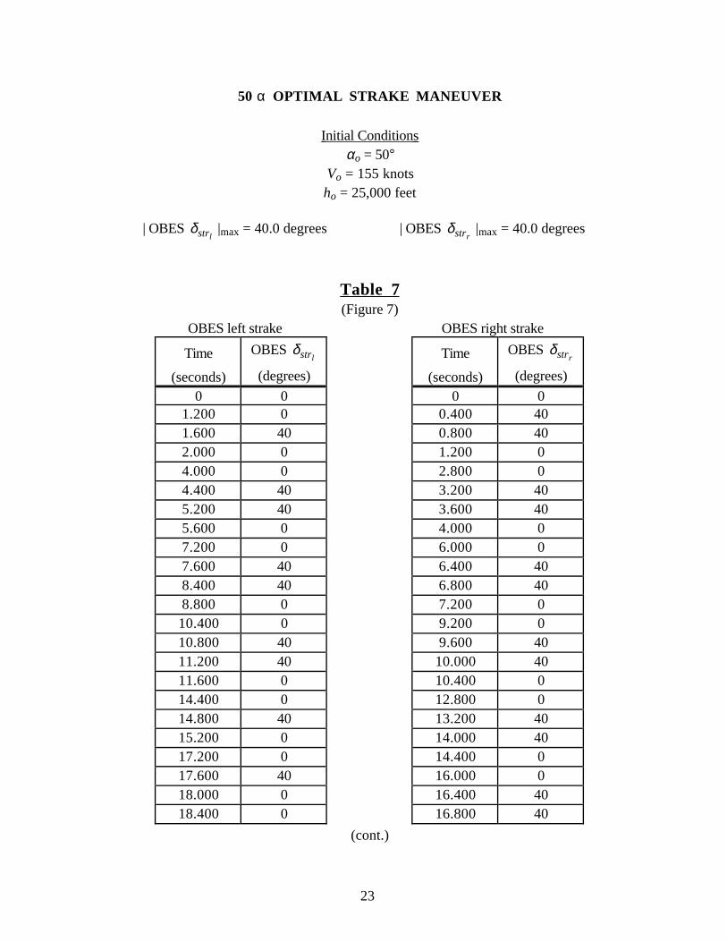
For the second maneuver, initial flight condition is trim angle of attack 50 degrees andapproximately 25,000 feet altitude, with the ANSER control law in TV mode. This maneuverinvolves independent deflection of the left and right strakes for studying individual strakeeffectiveness. Input specifications for the left / right strake optimal square wave input are given inTable 7. Figure 7 shows time histories for the optimal strake inputs. The inputs included a rate limitof 100 degrees/second for both left and right strakes
Both maneuvers in this group are to be flown two (2) times, for a total of four (4) runs. Eachrun should be preceded by at least two seconds of steady trimmed flight, and followed by at least twoseconds of free response before the pilot takes action to control the aircraft. The duration of eachmaneuver is 24 seconds. Estimated flight time for this set of maneuvers (including repeats) isapproximately 10 minutes.
3. This group of six maneuvers is for studying lateral dynamics and control effectiveness at highangle of attack. There are three different types of maneuver in this group. A maneuver of each typewas designed for two initial flight conditions:
a.) Trim angle of attack 40 degrees and approximately 25,000 feet altitude, with the ANSERcontrol law in TV mode.
b.) Trim angle of attack 50 degrees and approximately 25,000 feet altitude, with the ANSERcontrol law in TV mode.

8
A description of each maneuver type and the corresponding input specifications for the two flightconditions listed above are given next.
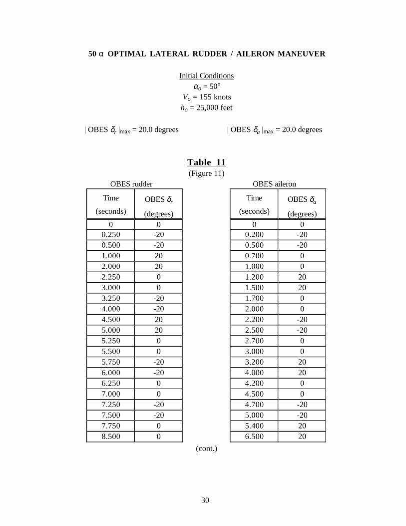
The first maneuver type involves simultaneous deflection of the rudder and aileron for studyinglateral dynamic response and for model updates and verification. Input specifications for therudder / aileron optimal square wave inputs are given in Table 8 for 40 degrees angle of attack, andin Table 11 for 50 degrees angle of attack. Figures 8 and 11 show time histories of the optimalinputs for 40 degrees angle of attack and 50 degrees angle of attack, respectively. All inputs includedrate limits of 82 degrees/second for rudder and 100 degrees/second for aileron.
The second maneuver type involves simultaneous deflection of the yaw thrust vectoring anddifferential strake for studying yaw thrust vectoring effectiveness and differential strakeeffectiveness, and for model updates and verification. A symmetric strake deflection must be appliedslowly before the start of this maneuver. The symmetric strake deflection δsstr is computed as:
δsstr = ( αo – 30) degrees for αo > 30 degrees
or,
δsstr = 10 degrees for αo = 40 degrees
δsstr = 20 degrees for αo = 50 degrees
Input specifications for the yaw thrust vectoring / differential strake optimal square wave inputs aregiven in Table 9 for 40 degrees angle of attack, and in Table 12 for 50 degrees angle of attack.Individual strake deflections are non-negative and are computed by combining the symmetric strakedeflection δsstr with the differential strake deflections δdstr from Tables 9 and 12, using thefollowing logic:
if (abs( δdstr ) ≤ 2.0*( δsstr )) then
δstrl = δsstr – 0.5*( δdstr )
δstrr = δsstr + 0.5*( δdstr )
else
if ( δdstr > 0.0) then
δstrl = 0.0
δstrr = δdstr
else
δstrl = – δdstr

9
δstrr = 0.0
end if
end if
Figures 9 and 12 show time histories of the optimal inputs for 40 degrees angle of attack and 50degrees angle of attack, respectively. All inputs included rate limits of 100 degrees/second for yawthrust vectoring and 180 degrees/second for differential strake.
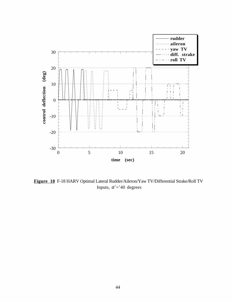
The third maneuver type involves sequential deflection of the rudder, aileron, yaw thrustvectoring, differential strake, and roll thrust vectoring for studying control effectiveness and optimalinput design, and for model updates and verification. A symmetric strake deflection must be appliedslowly before the start of this maneuver. The symmetric strake deflection δsstr is computed as:
δsstr = ( αo – 30) degrees for αo > 30 degrees
or,
δsstr = 10 degrees for αo = 40 degrees
δsstr = 20 degrees for αo = 50 degrees
Input specifications for the rudder / aileron / yaw thrust vectoring / differential strake / roll thrustvectoring optimal square wave inputs are given in Table 10 for 40 degrees angle of attack, and inTable 13 for 50 degrees angle of attack. Individual strake deflections are computed exactly asdescribed above for the second maneuver type in this set. Figures 10 and 13 show time histories ofthe optimal inputs for 40 degrees angle of attack and 50 degrees angle of attack, respectively. Allinputs included rate limits of 82 degrees/second for rudder, 100 degrees/second for aileron,100 degrees/second for yaw thrust vectoring, 180 degrees/second for differential strake, and100 degrees/second for roll thrust vectoring.
Each of the six maneuvers in this group is to be flown two (2) times, for a total of twelve (12)runs. Each run should be preceded by at least two seconds of steady trimmed flight, and followed byat least two seconds of free response before the pilot takes action to control the aircraft. The durationof the rudder / aileron maneuvers and the yaw thrust vectoring / differential strake maneuvers is 15seconds. The duration of the sequential rudder / aileron / yaw thrust vectoring / differentialstrake / roll thrust vectoring maneuvers is 21 seconds. Estimated flight time for this set ofmaneuvers (including repeats) is approximately 20 minutes.

10
III. Acknowledgments
This research was conducted at the NASA Langley Research Center under NASA contractNAS1-19000.
IV. References
1 . Gilbert, W.P. and Gatlin, D.H. "Review of the NASA High-Alpha Technology Program",NASA CP 3149, Volume I, Part I, High Angle-of-Attack Technology Conference, NASALangley Research Center, Hampton, Virginia. October 30 - November 1, 1990, pp. 23-59.
2 . Morelli, E. A. and Klein, V. "Optimal Input Design for Aircraft Parameter Estimation usingDynamic Programming Principles", AIAA paper 90-2801, Atmospheric Flight MechanicsConference, Portland, Oregon. August 1990.
3 . Morelli, E. A. "Practical Input Optimization for Aircraft Parameter Estimation Experiments",NASA CR 191462. May 1993.
4 . Wichman, K.D. and Earls, M. "On-Board Excitation System Specification for the F-18HARV", F-18 HARV Internal Document 91-84-101 (Rev. A), NASA Dryden Flight ResearchFacility, Edwards, California. July 1991.
5 . Messina, M.D. et al. "F/A-18 High Angle-of-Attack Research Vehicle SimulationModifications to Assist the Design of Advanced Control Laws", NASA TM 110216, NASALangley Research Center, Hampton, Virginia. 1996.
6 . Morelli, E.A. "Flight Test Validation of Optimal Input Design using Pilot Implementation",IFAC paper IFAC-559, 10th IFAC Symposium on System Identification, Copenhagen,Denmark. July 1994.
7 . Bacon, B.J., Davidson, J.B., Hoffler, K.D., Lallman, F.J., Messina, M.D., Murphy, P.C.,Ostroff, A.J., Proffitt, M.S., Strickland, M.E., Yeager, J.C., Foster, J. V., andBundick, W.T. "Design Specification for a Thrust-Vectoring, Actuated-Nose-Strake FlightControl Law for the High-Alpha Research Vehicle", NASA TM 110217, NASA LangleyResearch Center, Hampton, Virginia. 1996.
8 . Davidson, J.B., Foster, J.V., Ostroff, A.J., Lallman, F.J., Murphy, P.C., Hoffler, K.D., andMessina, M.D. "Development of a Control Law Design Process Utilizing Advanced SynthesisMethods with Application to the NASA F-18 HARV", NASA CP-3137, Volume 4, High-Angle-of-Attack Projects and Technology Conference, NASA Dryden Flight Research Facility,Edwards, California. April 21-23, 1992, pp. 111-158.

11
V. Input Specification Tables

12
5 α 3-2-1-1 LONGITUDINAL STABILATOR MANEUVER
Initial Conditions αo = 5°
Vo = 370 knotsho = 25,000 feet
| OBES δs |max = 3.0 degrees
Table 1(Figure 1)
OBES stabilator
Time(seconds)
OBES δs
(degrees)0 0
0.025 33.000 33.050 -35.000 -35.050 36.000 36.050 -37.000 -37.025 012.000 012.025 -315.000 -315.050 317.000 317.050 -318.000 -318.050 319.000 319.025 024.000 0

13
5 α OPTIMAL LONGITUDINAL STABILATOR MANEUVER
Initial Conditions αo = 5°
Vo = 370 knotsho = 25,000 feet
| OBES δs |max = 4.0 degrees
Table 2(Figure 2)
OBES stabilator
Time
(seconds)
OBES δs
(degrees)0 0
0.100 42.500 42.700 -43.000 -43.200 43.500 43.700 -46.000 -46.200 46.500 46.700 -47.000 -47.200 49.750 49.950 -410.250 -410.450 410.750 410.950 -413.250 -413.450 4
(cont.)

14
Table 2 (cont.)(Figure 2)
OBES stabilator
Time
(seconds)
OBES δs
(degrees)13.750 413.950 -414.250 -414.450 417.000 417.200 -417.500 -417.700 418.000 418.200 -420.000 -420.200 420.500 420.700 -421.000 -421.200 422.250 422.450 -422.750 -422.950 423.250 423.450 -423.750 -423.850 024.000 0

15
5 α 3-2-1-1 LATERAL RUDDER / AILERON MANEUVER
Initial Conditions αo = 5°
Vo = 370 knotsho = 25,000 feet
| OBES δr |max = 4.0 degrees | OBES δa |max = 2.5 degrees
Table 3(Figure 3)
OBES rudder OBES aileron
Time
(seconds)
OBES δr
(degrees)
Time
(seconds)
OBES δa
(degrees)0 0 0 0
0.050 4 10.000 02.675 4 10.025 -2.52.775 -4 12.675 -2.54.475 -4 12.725 2.54.575 4 14.475 2.55.375 4 14.525 -2.55.475 -4 15.375 -2.56.275 -4 15.425 2.56.325 0 16.275 2.520.000 0 16.300 0
20.000 0

16
5 α SEQUENTIAL OPTIMAL LATERAL RUDDER / AILERON MANEUVER
Initial Conditions αo = 5°
Vo = 370 knotsho = 25,000 feet
| OBES δr |max = 4.0 degrees | OBES δa |max = 2.5 degrees
Table 4(Figure 4)
OBES rudder OBES aileron
Time
(seconds)
OBES δr
(degrees)
Time
(seconds)
OBES δa
(degrees)0 0 0 0
0.075 4 10.125 00.900 4 10.150 -2.50.975 0 11.925 -2.51.125 0 11.975 2.51.200 4 13.050 2.51.575 4 13.100 -2.51.650 0 14.400 -2.52.025 0 14.450 2.52.100 4 18.000 2.52.475 4 18.025 02.550 0 18.450 02.700 0 18.475 -2.52.775 4 19.800 -2.53.600 4 19.825 03.675 0 20.000 03.825 03.900 44.050 44.175 -46.075 -4
(cont.)

17
Table 4 (cont.)(Figure 4)
OBES rudder
Time
(seconds)
OBES δr
(degrees)6.200 47.200 47.325 -47.425 -47.500 07.650 07.725 -47.875 -47.950 08.100 08.175 48.775 48.900 -410.125 -410.200 020.000 0

18
5 α OPTIMAL LATERAL RUDDER / AILERON MANEUVER
Initial Conditions αo = 5°
Vo = 370 knotsho = 25,000 feet
| OBES δr |max = 4.0 degrees | OBES δa |max = 2.5 degrees
Table 5(Figure 5)
OBES rudder OBES aileron
Time
(seconds)
OBES δr
(degrees)
Time
(seconds)
OBES δa
(degrees)0 0 0 0
0.075 -4 0.025 2.50.225 -4 1.125 2.50.300 0 1.175 -2.50.450 0 1.350 -2.50.525 -4 1.400 2.51.350 -4 1.800 2.51.475 4 1.850 -2.51.800 4 2.475 -2.51.875 0 2.525 2.52.025 0 3.150 2.52.100 4 3.200 -2.52.250 4 5.175 -2.52.375 -4 5.200 02.700 -4 5.400 02.825 4 5.425 2.52.925 4 9.225 2.53.050 -4 9.250 04.500 -4 9.450 04.625 4 9.475 -2.54.725 4 11.250 -2.5
(cont.)

19
Table 5 (cont.)(Figure 5)
OBES rudder OBES aileron
Time
(seconds)
OBES δr
(degrees)
Time
(seconds)
OBES δa
(degrees)4.800 0 11.300 2.54.950 0 11.925 2.55.025 4 11.975 -2.56.075 4 13.725 -2.56.200 -4 13.775 2.56.300 -4 14.625 2.56.375 0 14.650 06.525 0 14.850 06.600 -4 14.875 -2.56.975 -4 15.750 -2.57.050 0 15.800 2.57.200 0 17.775 2.57.275 4 17.825 -2.57.875 4 18.675 -2.58.000 -4 18.725 2.58.775 -4 19.800 2.58.850 0 19.825 09.000 0 20.000 09.075 49.900 410.025 -411.475 -411.550 011.700 011.775 412.150 412.225 012.375 012.450 412.600 412.725 -412.825 -4
(cont.)

20
Table 5 (cont.)(Figure 5)
OBES rudder
Time
(seconds)
OBES δr
(degrees)12.950 413.050 413.175 -414.400 -414.525 414.850 414.925 015.075 015.150 416.200 416.325 -416.650 -416.775 416.875 417.000 -417.325 -417.400 017.775 017.850 418.000 418.125 -418.225 -418.350 419.350 419.475 -419.575 -419.700 419.800 419.875 020.000 0

21
40 α OPTIMAL STRAKE MANEUVER
Initial Conditions αo = 40°
Vo = 155 knotsho = 25,000 feet
| OBES δstrl |max = 30.0 degrees | OBES δstrr
|max = 30.0 degrees
Table 6(Figure 6)
OBES left strake OBES right strake
Time
(seconds)
OBES δstrl
(degrees)
Time
(seconds)
OBES δstrr
(degrees)
0 0 0 00.900 0 0.300 301.200 30 0.600 301.500 0 0.900 03.000 0 4.800 03.300 30 5.100 303.600 30 5.400 303.900 0 5.700 05.700 0 6.600 06.000 30 6.900 306.300 0 7.500 307.800 0 7.800 08.100 30 10.500 08.400 0 10.800 309.000 0 11.400 309.300 30 11.700 09.900 30 12.900 010.200 0 13.200 3011.700 0 13.500 3012.000 30 13.800 012.300 30 15.000 012.600 0 15.300 3013.800 0 16.200 30
(cont.)

22
Table 6 (cont.)(Figure 6)
OBES left strake OBES right strake
Time
(seconds)
OBES δstrl
(degrees)
Time
(seconds)
OBES δstrr
(degrees)
14.100 30 16.500 014.400 30 18.300 014.700 0 18.600 3016.500 0 18.900 3016.800 30 19.200 017.700 30 20.400 018.000 0 20.700 3019.200 0 21.000 3019.500 30 21.300 019.800 30 24.000 020.100 021.300 021.600 3021.900 022.200 022.500 3022.800 3023.100 024.000 0
23
50 α OPTIMAL STRAKE MANEUVER
Initial Conditions αo = 50°
Vo = 155 knotsho = 25,000 feet
| OBES δstrl |max = 40.0 degrees | OBES δstrr
|max = 40.0 degrees
Table 7(Figure 7)
OBES left strake OBES right strake
Time
(seconds)
OBES δstrl
(degrees)
Time
(seconds)
OBES δstrr
(degrees)
0 0 0 01.200 0 0.400 401.600 40 0.800 402.000 0 1.200 04.000 0 2.800 04.400 40 3.200 405.200 40 3.600 405.600 0 4.000 07.200 0 6.000 07.600 40 6.400 408.400 40 6.800 408.800 0 7.200 010.400 0 9.200 010.800 40 9.600 4011.200 40 10.000 4011.600 0 10.400 014.400 0 12.800 014.800 40 13.200 4015.200 0 14.000 4017.200 0 14.400 017.600 40 16.000 018.000 0 16.400 4018.400 0 16.800 40
(cont.)

24
Table 7 (cont.)(Figure 7)
OBES left strake OBES right strake
Time
(seconds)
OBES δstrl
(degrees)
Time
(seconds)
OBES δstrr
(degrees)
18.800 40 17.200 019.200 40 24.000 019.600 022.800 023.200 4023.600 4024.000 0

25
40 α OPTIMAL LATERAL RUDDER / AILERON MANEUVER
Initial Conditions αo = 40°
Vo = 155 knotsho = 25,000 feet
| OBES δr |max = 18.0 degrees | OBES δa |max = 20.0 degrees
Table 8(Figure 8)
OBES rudder OBES aileron
Time
(seconds)
OBES δr
(degrees)
Time
(seconds)
OBES δa
(degrees)0 0 0 0
0.2000 18 0.2500 200.5000 18 0.5000 200.7000 0 0.7500 01.0000 0 1.0000 01.2000 -18 1.2500 -201.5000 -18 3.5000 -201.7000 0 4.0000 202.0000 0 4.5000 202.2000 -18 5.0000 -202.5000 -18 6.5000 -202.7000 0 7.0000 203.0000 0 8.5000 203.2000 18 8.7500 03.5000 18 9.0000 03.7000 0 9.2500 204.0000 0 10.0000 204.2000 -18 10.2500 04.5000 -18 10.5000 04.8750 18 10.7500 205.0000 18 12.5000 20
(cont.)

26
Table 8 (cont.)(Figure 8)
OBES rudder OBES aileron
Time
(seconds)
OBES δr
(degrees)
Time
(seconds)
OBES δa
(degrees)5.3750 -18 12.7500 05.5000 -18 13.0000 05.8750 18 13.2500 -206.5000 18 14.0000 -206.7000 0 14.5000 207.0000 0 14.5500 207.2000 -18 14.7500 08.0000 -18 15.0000 08.2000 08.5000 08.7000 189.0000 189.2000 09.5000 09.7000 1810.5000 1810.8750 -1811.5000 -1811.7000 013.0000 013.2000 1813.5000 1813.8750 -1814.5000 -1814.7000 015.0000 0

27
40 α OPTIMAL LATERAL YAW TV / DIFFERENTIAL STRAKE MANEUVER
Initial Conditions αo = 40°
Vo = 155 knotsho = 25,000 feet
| OBES δytv |max = 6.0 degrees | OBES δdstr |max = 20.0 degrees
Table 9(Figure 9)
OBES yaw thrust vectoring OBES differential strake
Time
(seconds)
OBES δytv
(degrees)
Time
(seconds)
OBES δdstr
(degrees)0 0 0 0
0.0750 6 0.1250 -200.4500 6 0.3000 -200.5750 -6 0.4250 00.7500 -6 0.9000 00.8750 6 1.0250 201.0500 6 1.2000 201.1750 -6 1.4250 -202.2500 -6 1.8000 -202.3750 6 2.0250 202.8500 6 2.7000 202.9250 0 2.9250 -203.1500 0 3.0000 -203.2250 6 3.2250 204.2000 6 3.4500 204.3250 -6 3.5750 05.2500 -6 3.7500 05.3250 0 3.8750 205.7000 0 4.5000 205.7750 6 4.7250 -206.4500 6 5.8500 -206.5250 0 5.9750 06.7500 0 6.3000 0
(cont.)

28
Table 9 (cont.)(Figure 9)
OBES yaw thrust vectoring OBES differential strake
Time
(seconds)
OBES δytv
(degrees)
Time
(seconds)
OBES δdstr
(degrees)6.8250 6 6.4250 -207.0500 6 6.6000 -207.1750 -6 6.8250 208.2500 -6 8.1000 208.3250 0 8.2250 08.5500 0 8.4000 08.6250 6 8.5250 -209.1500 6 9.6000 -209.2250 0 9.7250 09.9000 0 9.9000 09.9750 -6 10.0250 -2010.8000 -6 10.3500 -2010.8750 0 10.5750 2011.1000 0 10.8000 2011.1750 -6 10.9250 011.4000 -6 11.1000 011.5250 6 11.2250 -2011.7000 6 11.5500 -2011.8250 -6 11.7750 2012.0000 -6 12.0000 2012.1250 6 12.1250 013.0500 6 12.6000 013.1250 0 12.7250 2013.3500 0 13.6500 2013.4250 6 13.7750 014.7000 6 13.9500 014.7750 0 14.0750 2015.0000 0 14.2500 20
14.4750 -2014.7000 -2014.8250 015.0000 0

29
40 α OPTIMAL LATERAL SEQUENTIAL MANEUVER
Initial Conditions αo = 40°
Vo = 155 knotsho = 25,000 feet
| OBES δr |max = 19.0 degrees | OBES δa |max = 18.0 degrees
| OBES δytv |max = 6.0 degrees | OBES δdstr |max = 20.0 degrees
| OBES δrtv |max = 10.0 degrees
Table 10(Figure 10)
OBES rudder OBES aileron OBES yaw TV OBES diff. strake OBES roll TV
Time
(sec)
OBES
δr
(deg)
Time
(sec)
OBES
δa
(deg)
Time
(sec)
OBES
δytv
(deg)
Time
(sec)
OBES
δdstr
(deg)
Time
(sec)
OBES
δrtv
(deg)
0 0 0 0 0 0 0 0 0 0
0.250 19 4.000 0 8.000 0 12.000 0 16.000 0
0.500 19 4.200 18 8.075 6 12.125 20 16.100 -10
0.750 0 4.500 18 9.500 6 12.500 20 17.000 -10
1.000 0 4.875 -18 9.625 -6 12.725 -20 17.100 0
1.250 19 5.000 -18 11.000 -6 13.500 -20 17.500 0
1.500 19 5.375 18 11.075 0 13.625 0 17.600 10
1.975 -19 5.500 18 11.500 0 14.000 0 18.000 10
2.000 -19 5.875 -18 11.575 6 14.125 20 18.100 0
2.475 19 6.000 -18 12.000 6 15.000 20 18.500 0
2.500 19 6.200 0 12.075 0 15.225 -20 18.600 10
2.975 -19 6.500 0 21.000 0 15.500 -20 19.500 10
3.000 -19 6.700 -18 15.625 0 19.700 -10
3.250 0 7.000 -18 21.000 0 20.000 -10
3.500 0 7.375 18 20.100 0
3.750 19 8.000 18 21.000 0
4.000 19 8.200 0
4.250 0 21.000 0
21.000 0
30
50 α OPTIMAL LATERAL RUDDER / AILERON MANEUVER
Initial Conditions αo = 50°
Vo = 155 knotsho = 25,000 feet
| OBES δr |max = 20.0 degrees | OBES δa |max = 20.0 degrees
Table 11(Figure 11)
OBES rudder OBES aileron
Time
(seconds)
OBES δr
(degrees)
Time
(seconds)
OBES δa
(degrees)0 0 0 0
0.250 -20 0.200 -200.500 -20 0.500 -201.000 20 0.700 02.000 20 1.000 02.250 0 1.200 203.000 0 1.500 203.250 -20 1.700 04.000 -20 2.000 04.500 20 2.200 -205.000 20 2.500 -205.250 0 2.700 05.500 0 3.000 05.750 -20 3.200 206.000 -20 4.000 206.250 0 4.200 07.000 0 4.500 07.250 -20 4.700 -207.500 -20 5.000 -207.750 0 5.400 208.500 0 6.500 20
(cont.)

31
Table 11 (cont.)(Figure 11)
OBES rudder OBES aileron
Time
(seconds)
OBES δr
(degrees)
Time
(seconds)
OBES δa
(degrees)8.750 20 6.900 -209.500 20 7.500 -209.750 0 7.700 010.000 0 8.000 010.250 20 8.200 2010.500 20 8.500 2010.750 0 8.900 -2013.000 0 9.000 -2013.250 -20 9.200 013.500 -20 9.500 013.750 0 9.700 -2015.000 0 10.500 -20
10.700 011.000 011.200 -2011.500 -2011.900 2012.000 2012.200 012.500 012.700 -2013.000 -2013.200 013.500 013.700 -2014.000 -2014.400 2014.500 2014.700 015.000 0

32
50 α OPTIMAL LATERAL YAW TV / DIFFERENTIAL STRAKE MANEUVER
Initial Conditions αo = 50°
Vo = 155 knotsho = 25,000 feet
| OBES δytv |max = 5.0 degrees | OBES δdstr |max = 15.0 degrees
Table 12(Figure 12)
OBES yaw thrust vectoring OBES differential strake
Time
(seconds)
OBES δytv
(degrees)
Time
(seconds)
OBES δdstr
(degrees)0 0 0 0
0.050 5 0.100 150.800 5 0.800 150.850 0 0.975 -151.000 0 2.000 -151.050 -5 2.175 151.200 -5 2.200 151.250 0 2.375 -151.400 0 2.600 -151.450 -5 2.775 151.800 -5 3.400 151.900 5 3.575 -152.000 5 4.800 -152.050 0 4.975 152.400 0 5.600 152.450 5 5.775 -152.600 5 5.800 -152.700 -5 5.900 02.800 -5 6.000 02.850 0 6.100 -153.000 0 6.200 -153.050 -5 6.300 03.600 -5 6.400 03.700 5 6.500 -15
(cont.)

33
Table 12 (cont.)(Figure 12)
OBES yaw thrust vectoring OBES differential strake
Time
(seconds)
OBES δytv
(degrees)
Time
(seconds)
OBES δdstr
(degrees)4.200 5 6.800 -154.250 0 6.975 154.400 0 7.200 154.450 -5 7.375 -156.000 -5 9.200 -156.100 5 9.300 08.200 5 9.400 08.300 -5 9.500 -158.800 -5 10.200 -158.850 0 10.375 159.000 0 10.800 159.050 -5 10.900 09.200 -5 11.200 09.300 5 11.300 1510.800 5 12.000 1510.900 -5 12.175 -1511.200 -5 13.600 -1511.250 0 13.775 1511.600 0 14.800 1511.650 -5 14.900 011.800 -5 15.000 011.850 012.000 012.050 -512.200 -512.300 512.400 512.500 -512.600 -512.700 514.800 514.850 015.000 0

34
50 α OPTIMAL LATERAL SEQUENTIAL MANEUVER
Initial Conditions αo = 50°
Vo = 155 knotsho = 25,000 feet
| OBES δr |max = 19.0 degrees | OBES δa |max = 20.0 degrees
| OBES δytv |max = 5.0 degrees | OBES δdstr |max = 20.0 degrees
| OBES δrtv |max = 10.0 degrees
Table 13(Figure 13)
OBES rudder OBES aileron OBES yaw TV OBES diff. strake OBES roll TV
Time
(sec)
OBES
δr
(deg)
Time
(sec)
OBES
δa
(deg)
Time
(sec)
OBES
δytv
(deg)
Time
(sec)
OBES
δdstr
(deg)
Time
(sec)
OBES
δrtv
(deg)
0 0 0 0 0 0 0 0 0 0
0.250 -19 4.000 0 8.000 0 12.000 0 16.000 0
2.500 -19 4.200 20 8.050 5 12.125 -20 16.100 10
2.975 19 4.500 20 9.500 5 14.000 -20 17.000 10
3.000 19 4.900 -20 9.600 -5 14.225 20 17.200 -10
3.250 0 5.500 -20 10.500 -5 16.000 20 18.000 -10
3.500 0 5.900 20 10.600 5 16.125 0 18.100 0
3.750 -19 6.500 20 11.000 5 21.000 0 18.500 0
4.000 -19 6.900 -20 11.050 0 18.600 10
4.250 0 7.500 -20 11.500 0 20.000 10
21.000 0 7.900 20 11.550 5 20.100 0
8.000 20 12.000 5 21.000 0
8.200 0 12.050 0
21.000 0 21.000 0

35
VI. Control Time Histories
-4
-3
-2
-1
0
1
2
3
4
0 4 8 12 16 20 24
sym
met
ric
stab
ilat
or
(deg
)
time (sec)
Figure 1 F-18 HARV 3-2-1-1 Longitudinal Stabilator Input, α = 5 degrees

36
-5
-4
-3
-2
-1
0
1
2
3
4
5
0 4 8 12 16 20 24
sym
met
ric
stab
ilat
or
(deg
)
time (sec)
Figure 2 F-18 HARV Optimal Longitudinal Stabilator Input, α = 5 degrees
37
-5
-4
-3
-2
-1
0
1
2
3
4
5
0 5 10 15 20
rudd
er
(deg
)
time (sec)
-5
-4
-3
-2
-1
0
1
2
3
4
5
0 5 10 15 20
aile
ron
(d
eg)
time (sec)
Figure 3 F-18 HARV 3-2-1-1 Lateral Rudder/Aileron Inputs, α = 5 degrees

38
-5
-4
-3
-2
-1
0
1
2
3
4
5
0 5 10 15 20
rudd
er
(deg
)
time (sec)
-5
-4
-3
-2
-1
0
1
2
3
4
5
0 5 10 15 20
aile
ron
(d
eg)
time (sec)
Figure 4 F-18 HARV Sequential Optimal Lateral Rudder/Aileron Inputs, α = 5 degrees

39
-5
-4
-3
-2
-1
0
1
2
3
4
5
0 5 10 15 20
rudd
er
(deg
)
time (sec)
-5
-4
-3
-2
-1
0
1
2
3
4
5
0 5 10 15 20
aile
ron
(d
eg)
time (sec)
Figure 5 F-18 HARV Optimal Lateral Rudder/Aileron Inputs, α = 5 degrees

40
0
5
10
15
20
25
30
35
0 4 8 12 16 20 24
left
str
ake
(de
g)
time (sec)
0
5
10
15
20
25
30
35
0 4 8 12 16 20 24
righ
t st
rake
(d
eg)
time (sec)
Figure 6 F-18 HARV Optimal Lateral Left/Right Strake Inputs, α = 40 degrees

41
0
10
20
30
40
50
0 4 8 12 16 20 24
left
str
ake
(de
g)
time (sec)
0
10
20
30
40
50
0 4 8 12 16 20 24
righ
t st
rake
(d
eg)
time (sec)
Figure 7 F-18 HARV Optimal Lateral Left/Right Strake Inputs, α = 50 degrees

42
-30
-20
-10
0
10
20
30
0 5 10 15
rudd
er
(deg
)
time (sec)
-20
-15
-10
-5
0
5
10
15
20
0 5 10 15
aile
ron
(d
eg)
time (sec)
Figure 8 F-18 HARV Optimal Lateral Rudder/Aileron Inputs, α = 40 degrees

43
-8
-6
-4
-2
0
2
4
6
8
0 5 10 15
yaw
th
rust
vec
tori
ng
(d
eg)
time (sec)
-30
-20
-10
0
10
20
30
0 5 10 15
dif
fere
nti
al s
trak
e (
deg
)
time (sec)
Figure 9 F-18 HARV Optimal Lateral Yaw TV/Differential Strake Inputs, α = 40 degrees
44
-30
-20
-10
0
10
20
30
0 5 10 15 20
rudderaileronyaw TVdiff. strakeroll TV
con
trol
def
lect
ion
(d
eg)
time (sec)
Figure 10 F-18 HARV Optimal Lateral Rudder/Aileron/Yaw TV/Differential Strake/Roll TVInputs, α = 40 degrees

45
-30
-20
-10
0
10
20
30
0 5 10 15
rudd
er
(deg
)
time (sec)
-30
-20
-10
0
10
20
30
0 5 10 15
aile
ron
(d
eg)
time (sec)
Figure 11 F-18 HARV Optimal Lateral Rudder/Aileron Inputs, α = 50 degrees

46
-6
-4
-2
0
2
4
6
0 5 10 15
yaw
th
rust
vec
tori
ng
(d
eg)
time (sec)
-20
-15
-10
-5
0
5
10
15
20
0 5 10 15
dif
fere
nti
al s
trak
e (
deg
)
time (sec)
Figure 12 F-18 HARV Optimal Lateral Yaw TV/Differential Strake Inputs, α = 50 degrees

47
-30
-20
-10
0
10
20
30
0 5 10 15 20
rudderaileronyaw TVdiff. strakeroll TV
con
trol
def
lect
ion
(d
eg)
time (sec)
Figure 13 F-18 HARV Optimal Lateral Rudder/Aileron/Yaw TV/Differential Strake/Roll TVInputs, α = 50 degrees


![[Bản Việt Nam] Làm Giàu Nhanh - T. Harv Eker](https://img.dokumen.tips/doc/110x75/588a6b941a28ab336f8b5181/ban-viet-nam-lam-giau-nhanh-t-harv-eker.jpg)