Extraction of Tubular Structures over an Orientation Domain

Mickaël PéchaudLIENS

École Normale SupérieureParis, France

Renaud KerivenIMAGINE / LIGMUniversité Paris-Est

Paris, France

Gabriel PeyréCEREMADE

Université Paris DauphineParis, France

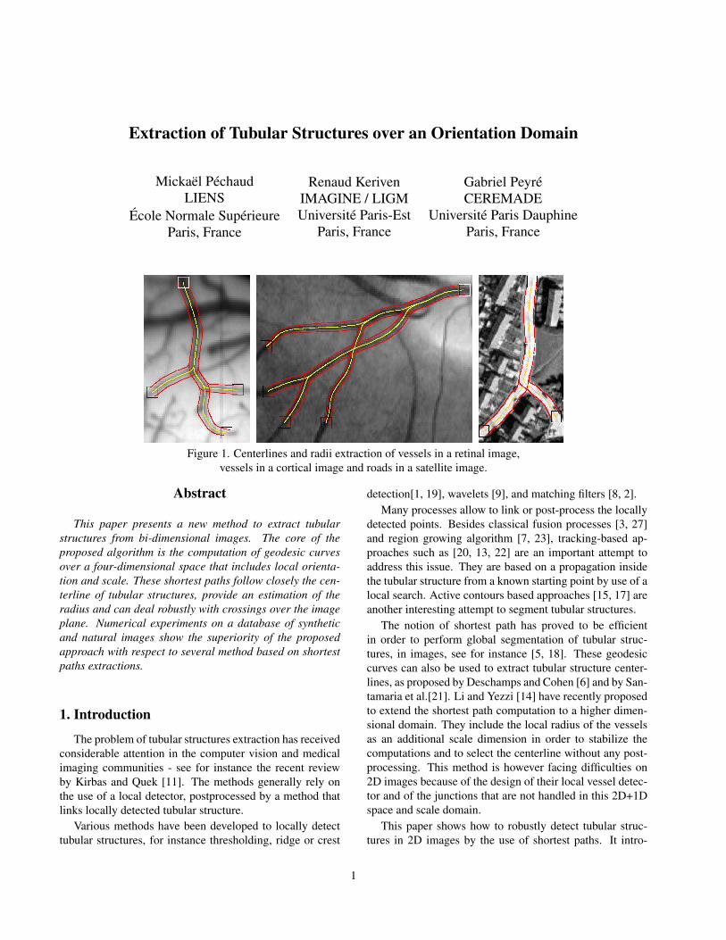
Figure 1. Centerlines and radii extraction of vessels in a retinal image,vessels in a cortical image and roads in a satellite image.

Abstract

This paper presents a new method to extract tubularstructures from bi-dimensional images. The core of theproposed algorithm is the computation of geodesic curvesover a four-dimensional space that includes local orienta-tion and scale. These shortest paths follow closely the cen-terline of tubular structures, provide an estimation of theradius and can deal robustly with crossings over the imageplane. Numerical experiments on a database of syntheticand natural images show the superiority of the proposedapproach with respect to several method based on shortestpaths extractions.

1. Introduction

The problem of tubular structures extraction has receivedconsiderable attention in the computer vision and medicalimaging communities - see for instance the recent reviewby Kirbas and Quek [11]. The methods generally rely onthe use of a local detector, postprocessed by a method thatlinks locally detected tubular structure.

Various methods have been developed to locally detecttubular structures, for instance thresholding, ridge or crest

detection[1, 19], wavelets [9], and matching filters [8, 2].Many processes allow to link or post-process the locally

detected points. Besides classical fusion processes [3, 27]and region growing algorithm [7, 23], tracking-based ap-proaches such as [20, 13, 22] are an important attempt toaddress this issue. They are based on a propagation insidethe tubular structure from a known starting point by use of alocal search. Active contours based approaches [15, 17] areanother interesting attempt to segment tubular structures.

The notion of shortest path has proved to be efficientin order to perform global segmentation of tubular struc-tures, in images, see for instance [5, 18]. These geodesiccurves can also be used to extract tubular structure center-lines, as proposed by Deschamps and Cohen [6] and by San-tamaria et al.[21]. Li and Yezzi [14] have recently proposedto extend the shortest path computation to a higher dimen-sional domain. They include the local radius of the vesselsas an additional scale dimension in order to stabilize thecomputations and to select the centerline without any post-processing. This method is however facing difficulties on2D images because of the design of their local vessel detec-tor and of the junctions that are not handled in this 2D+1Dspace and scale domain.

This paper shows how to robustly detect tubular struc-tures in 2D images by the use of shortest paths. It intro-

1

duces an additional local orientation dimension that disam-biguates the crossing singularities using pattern-recognitioninspired techniques. Centerline detection and radius esti-mation are completely embedded in the proposed segmen-tation method and does not rely on additional properties ofthe images (such as centerlines being the darker part of ves-sels), nor on a post-processing step. Numerical results onsynthetic and real-life examples shows the advantage of us-ing this orientation information. The database will availableonline so that future method can compare their results to theproposed approach.

2. Shortest paths in orientation domainThis paper considers a gray scale image I : [0, 1]2 →

[0, 1] and in numerical computation, this image is sampledregularly on a grid of n×n pixels. In the following, deriva-tive operators in the continuous domain are used althoughthe computations are done on the discrete grid using finitedifferences.

2.1. Local Tubular Structure Model

At the core of the proposed approach is the local de-tection of tubular structures. This paper uses a normalizedcross-correlation with a tubular model as a local feature in-dicator.

The local geometry of a tubular structure is capturedwith a model M(x) ∈ R for x = (x1, x2) ∈ Λ =[−Λ1,Λ1]× [−Λ2,Λ2]. The models considered is this arti-cle are of the form M(x1, x2) = m(x2) and therefore onlydepend on a 1D profile m. A model is thus a small tem-plate which represents a typical horizontal tubular structureof normalized width one wishes to detect. This normalizedpattern is then rotated and scaled in order to define warpedmodels Mr,θ(x) for x ∈ Λ(r, θ) = rRθ(Λ)

∀x ∈ Λ(r, θ), Mr,θ(x) def.= M(R−θ(x/r)) (1)

where Rθ is the planar rotation of angle θ. Each patternMr,θ looks like a typical tubular structure oriented alongdirection θ ∈ [0, π) and of width r > 0.

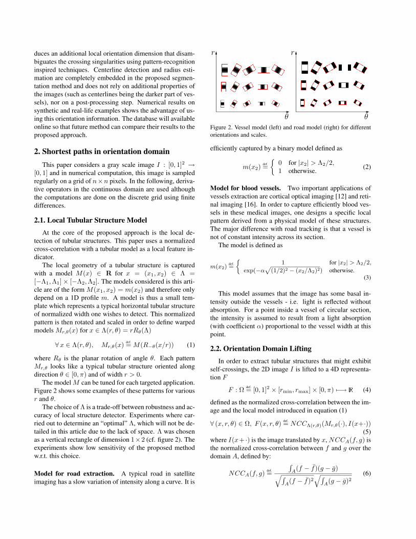
The model M can be tuned for each targeted application.Figure 2 shows some examples of these patterns for variousr and θ.

The choice of Λ is a trade-off between robustness and ac-curacy of local structure detector. Experiments where car-ried out to determine an “optimal” Λ, which will not be de-tailed in this article due to the lack of space. Λ was chosenas a vertical rectangle of dimension 1×2 (cf. figure 2). Theexperiments show low sensitivity of the proposed methodw.r.t. this choice.

Model for road extraction. A typical road in satelliteimaging has a slow variation of intensity along a curve. It is

θ θ

r r

Figure 2. Vessel model (left) and road model (right) for differentorientations and scales.

efficiently captured by a binary model defined as

m(x2)def.=

0 for |x2| > Λ2/2,1 otherwise. (2)

Model for blood vessels. Two important applications ofvessels extraction are cortical optical imaging [12] and reti-nal imaging [16]. In order to capture efficiently blood ves-sels in these medical images, one designs a specific localpattern derived from a physical model of these structures.The major difference with road tracking is that a vessel isnot of constant intensity across its section.

The model is defined as

m(x2)def.=

1 for |x2| > Λ2/2,

exp(−αp

(1/2)2 − (x2/Λ2)2) otherwise.(3)

This model assumes that the image has some basal in-tensity outside the vessels - i.e. light is reflected withoutabsorption. For a point inside a vessel of circular section,the intensity is assumed to result from a light absorption(with coefficient α) proportional to the vessel width at thispoint.

2.2. Orientation Domain Lifting

In order to extract tubular structures that might exhibitself-crossings, the 2D image I is lifted to a 4D representa-tion F

F : Ω def.= [0, 1]2 × [rmin, rmax]× [0, π) 7−→ R (4)

defined as the normalized cross-correlation between the im-age and the local model introduced in equation (1)

∀ (x, r, θ) ∈ Ω, F (x, r, θ) def.= NCCΛ(r,θ)(Mr,θ(·), I(x+·))(5)

where I(x+ ·) is the image translated by x, NCCA(f, g) isthe normalized cross-correlation between f and g over thedomain A, defined by:

NCCA(f, g) def.=

∫A(f − f)(g − g)√∫

A(f − f)2

√∫A(g − g)2

(6)

where h =R

Ah

µ(A) , µ(A) being the area of A.Function F ranges from −1 to 1, is invariant under local

intensity changes and is an indicator of how likely a tubularstructure of radius r and orientation θ is present at locationx.

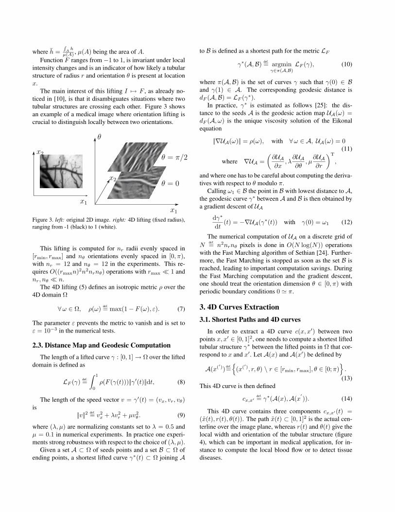
The main interest of this lifting I 7→ F , as already no-ticed in [10], is that it disambiguates situations where twotubular structures are crossing each other. Figure 3 showsan example of a medical image where orientation lifting iscrucial to distinguish locally between two orientations.

θ

x2θ = π/2

θ = 0

x1

x1

x2

Figure 3. left: original 2D image. right: 4D lifting (fixed radius),ranging from -1 (black) to 1 (white).

This lifting is computed for nr radii evenly spaced in[rmin, rmax] and nθ orientations evenly spaced in [0, π),with nr = 12 and nθ = 12 in the experiments. This re-quires O((rmaxn)2n2nrnθ) operations with rmax 1 andnr, nθ n.

The 4D lifting (5) defines an isotropic metric ρ over the4D domain Ω

∀ω ∈ Ω, ρ(ω) def.= max(1− F (ω), ε). (7)

The parameter ε prevents the metric to vanish and is set toε = 10−3 in the numerical tests.

2.3. Distance Map and Geodesic Computation

The length of a lifted curve γ : [0, 1] → Ω over the lifteddomain is defined as

LF (γ) def.=∫ 1

0

ρ(F (γ(t)))||γ′(t)||dt, (8)

The length of the speed vector v = γ′(t) = (vx, vr, vθ)is

||v||2 def.= v2x + λv2

r + µv2θ . (9)

where (λ, µ) are normalizing constants set to λ = 0.5 andµ = 0.1 in numerical experiments. In practice one experi-ments strong robustness with respect to the choice of (λ, µ).

Given a set A ⊂ Ω of seeds points and a set B ⊂ Ω ofending points, a shortest lifted curve γ∗(t) ⊂ Ω joining A

to B is defined as a shortest path for the metric LF

γ∗(A,B) def.= argminγ∈π(A,B)

LF (γ), (10)

where π(A,B) is the set of curves γ such that γ(0) ∈ Band γ(1) ∈ A. The corresponding geodesic distance isdF (A,B) = LF (γ∗).

In practice, γ∗ is estimated as follows [25]: the dis-tance to the seeds A is the geodesic action map UA(ω) =dF (A, ω) is the unique viscosity solution of the Eikonalequation

||∇UA(ω)|| = ρ(ω), with ∀ω ∈ A, UA(ω) = 0(11)

where ∇UA =(

∂UA∂x

, λ∂UA∂θ

, µ∂UA∂r

)T

,

and where one has to be careful about computing the deriva-tives with respect to θ modulo π.

Calling ω1 ∈ B the point in B with lowest distance to A,the geodesic curve γ∗ between A and B is then obtained bya gradient descent of UA

dγ∗

dt(t) = −∇UA(γ∗(t)) with γ(0) = ω1 (12)

The numerical computation of UA on a discrete grid ofN

def.= n2nrnθ pixels is done in O(N log(N)) operationswith the Fast Marching algorithm of Sethian [24]. Further-more, the Fast Marching is stopped as soon as the set B isreached, leading to important computation savings. Duringthe Fast Marching computation and the gradient descent,one should treat the orientation dimension θ ∈ [0, π) withperiodic boundary conditions 0 ' π.

3. 4D Curves Extraction3.1. Shortest Paths and 4D curves

In order to extract a 4D curve c(x, x′) between twopoints x, x′ ∈ [0, 1]2, one needs to compute a shortest liftedtubular structure γ∗ between the lifted points in Ω that cor-respond to x and x′. Let A(x) and A(x′) be defined by

A(x(′)) def.=

(x(′), r, θ) \ r ∈ [rmin, rmax], θ ∈ [0;π)

.

(13)This 4D curve is then defined

cx,x′def.= γ∗(A(x),A(x

′)). (14)

This 4D curve contains three components cx,x′(t) =(x(t), r(t), θ(t)). The path x(t) ⊂ [0, 1]2 is the actual cen-terline over the image plane, whereas r(t) and θ(t) give thelocal width and orientation of the tubular structure (figure4), which can be important in medical application, for in-stance to compute the local blood flow or to detect tissuediseases.

t

t

θ(t)

r(t)

Figure 4. Left: extraction of a vessel in a cortical image. Startingpoint: white square. Ending point: black square. Right: corre-sponding orientation θ(t) and radius r(t).

3.2. Numerical Experiments

3.2.1 Phantom experiments.

Experiments were carried out on several phantoms im-ages, for which the centerlines positions and the radii haveknown analytical forms with sub-pixelic accuracy. Thecross section of these phantoms corresponds to the model(3) with parameter α = 0.01. An additive Gaussian whitenoise with various amplitudes are added to the phantoms.Ten phantoms are generated for each condition, and eachnoise level, see Figure 5. In each case, the true starting andending points of each phantom are used, as well as the truestarting and ending radii for the [14] method. The result-ing benchmark database will be available online in order toallow comparison with future works.

Figure 5. Some of the sample phantoms used as benchmarks (basicintensities range from 0 to 1), shown here with a spatially indepen-dent Gaussian noise of variance 0.15.

For each phantom and level of noise, three algorithmswere tested: the classical 2D method Fast Marching [4]with pre-smoothing of the image (pre-smoothing is classi-cally used in Fast Marching based methods to obtain a cen-tered path), Li/Yezzi method[14] and the method proposedin this article. The smoothing parameter of the classical 2Dmethod, the smoothing parameter as well the three more pa-rameters of the 3D method were optimized for this bench-mark. In order not to take advantage of the exact knowledgeof the profile, the proposed method was applied with a vol-

untary wrong model parameter α = 0.1. In each case, thetrue starting and ending points of each phantom are used,as well as the true starting and ending radii for the [14]method.

For each method, the error of the vessels centerline po-sition and radius w.r.t the ground truth was computed usingthe following formula.

ErrorC(c)2 =∫ 1

0

||x(t)− x∗(t∗)||2dt (15)

where t∗ is such that x∗(t) is the ground truth centerlinepoint closest to the computed centerline x(t).

The error of the radii estimation ([14] and proposedmethod only) was computed using the following formula:

ErrorR(c)2 =∫ 1

0

|r(t)− r∗(t∗)|2 dt (16)

where r is the radius computed by the method, and r∗

the ground truth radius.Figure 6 shows ErrorC(c) and ErrorR(c) curves for sev-

eral synthetic images as a function of the noise level. Usingthe 3D space+scale lifting [14] produces results of varyingquality, and requires a careful tuning of the parameters toachieve the optimal error rate. [4] with an optimal smooth-ing provides a precise evaluation of the centerline locations,but without any evaluation of the local radius. The proposedmethod provides both positions and radii with more robust-ness and accuracy.

3.2.2 Real images experiments.

Figure 1 shows results of tubular structure extraction forthe three modalities considered in this paper:

Left: vessels extraction for a complex optical imaging ofthe cortex with several branches and intersections.Center: vessels extraction on a retinal image from theDRIVE database [26, 16].Right: road extracted from a satellite image over an urbanarea.

The starting areaA is shown with a white square and severalending points ω are shown with black squares.

The crossings in the retinal image (center) show the in-terest of the 4D lifting. Note also the large overlap of thecenterlines computed from several different points, the sub-pixelic precision of the centerline and the correct handlingof intersections on the cortical image (left).

Another interest of this method is that it automaticallycomputes the radius r(t) and orientation θ(t) parameters(figure 4).

The precision of the 4D lifting method is evaluated onthe DRIVE database [26, 16]. Approximate ground truthcenterlines positions and radii are computed from the binary

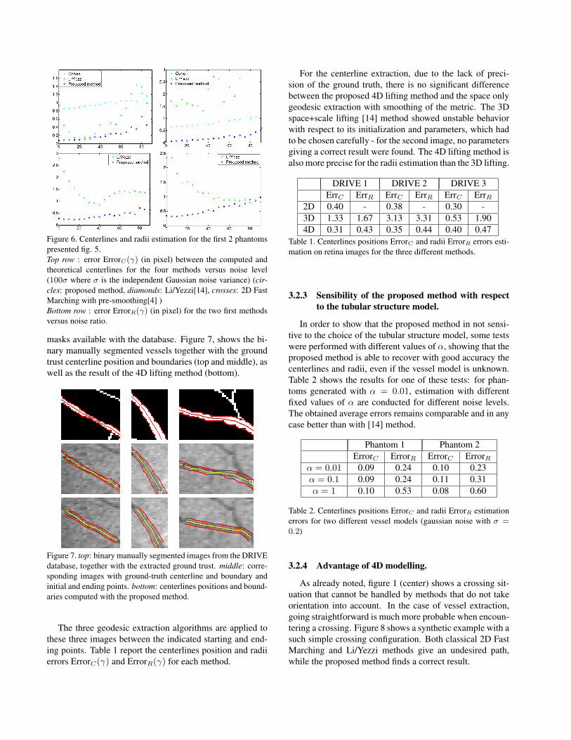
Figure 6. Centerlines and radii estimation for the first 2 phantomspresented fig. 5.Top row : error ErrorC(γ) (in pixel) between the computed andtheoretical centerlines for the four methods versus noise level(100σ where σ is the independent Gaussian noise variance) (cir-cles: proposed method, diamonds: Li/Yezzi[14], crosses: 2D FastMarching with pre-smoothing[4] )Bottom row : error ErrorR(γ) (in pixel) for the two first methodsversus noise ratio.

masks available with the database. Figure 7, shows the bi-nary manually segmented vessels together with the groundtrust centerline position and boundaries (top and middle), aswell as the result of the 4D lifting method (bottom).

Figure 7. top: binary manually segmented images from the DRIVEdatabase, together with the extracted ground trust. middle: corre-sponding images with ground-truth centerline and boundary andinitial and ending points. bottom: centerlines positions and bound-aries computed with the proposed method.

The three geodesic extraction algorithms are applied tothese three images between the indicated starting and end-ing points. Table 1 report the centerlines position and radiierrors ErrorC(γ) and ErrorR(γ) for each method.

For the centerline extraction, due to the lack of preci-sion of the ground truth, there is no significant differencebetween the proposed 4D lifting method and the space onlygeodesic extraction with smoothing of the metric. The 3Dspace+scale lifting [14] method showed unstable behaviorwith respect to its initialization and parameters, which hadto be chosen carefully - for the second image, no parametersgiving a correct result were found. The 4D lifting method isalso more precise for the radii estimation than the 3D lifting.

DRIVE 1 DRIVE 2 DRIVE 3ErrC ErrR ErrC ErrR ErrC ErrR

2D 0.40 - 0.38 - 0.30 -3D 1.33 1.67 3.13 3.31 0.53 1.904D 0.31 0.43 0.35 0.44 0.40 0.47

Table 1. Centerlines positions ErrorC and radii ErrorR errors esti-mation on retina images for the three different methods.

3.2.3 Sensibility of the proposed method with respectto the tubular structure model.

In order to show that the proposed method in not sensi-tive to the choice of the tubular structure model, some testswere performed with different values of α, showing that theproposed method is able to recover with good accuracy thecenterlines and radii, even if the vessel model is unknown.Table 2 shows the results for one of these tests: for phan-toms generated with α = 0.01, estimation with differentfixed values of α are conducted for different noise levels.The obtained average errors remains comparable and in anycase better than with [14] method.

Phantom 1 Phantom 2ErrorC ErrorR ErrorC ErrorR

α = 0.01 0.09 0.24 0.10 0.23α = 0.1 0.09 0.24 0.11 0.31α = 1 0.10 0.53 0.08 0.60

Table 2. Centerlines positions ErrorC and radii ErrorR estimationerrors for two different vessel models (gaussian noise with σ =0.2)

3.2.4 Advantage of 4D modelling.

As already noted, figure 1 (center) shows a crossing sit-uation that cannot be handled by methods that do not takeorientation into account. In the case of vessel extraction,going straightforward is much more probable when encoun-tering a crossing. Figure 8 shows a synthetic example with asuch simple crossing configuration. Both classical 2D FastMarching and Li/Yezzi methods give an undesired path,while the proposed method finds a correct result.

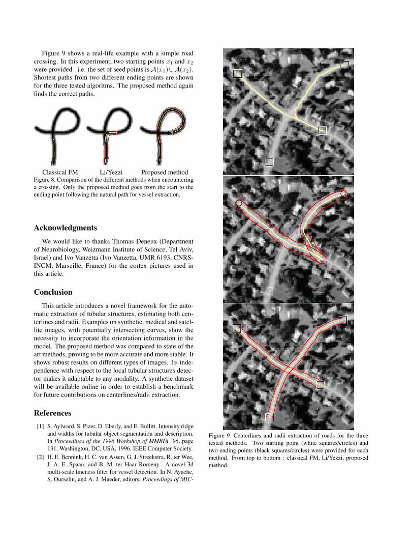
Figure 9 shows a real-life example with a simple roadcrossing. In this experiment, two starting points x1 and x2

were provided - i.e. the set of seed points isA(x1)∪A(x2).Shortest paths from two different ending points are shownfor the three tested algoritms. The proposed method againfinds the correct paths.

Classical FM Li/Yezzi Proposed methodFigure 8. Comparison of the different methods when encounteringa crossing. Only the proposed method goes from the start to theending point following the natural path for vessel extraction.

Acknowledgments

We would like to thanks Thomas Deneux (Departmentof Neurobiology, Weizmann Institute of Science, Tel Aviv,Israel) and Ivo Vanzetta (Ivo Vanzetta, UMR 6193, CNRS-INCM, Marseille, France) for the cortex pictures used inthis article.

Conclusion

This article introduces a novel framework for the auto-matic extraction of tubular structures, estimating both cen-terlines and radii. Examples on synthetic, medical and satel-lite images, with potentially intersecting curves, show thenecessity to incorporate the orientation information in themodel. The proposed method was compared to state of theart methods, proving to be more accurate and more stable. Itshows robust results on different types of images. Its inde-pendence with respect to the local tubular structures detec-tor makes it adaptable to any modality. A synthetic datasetwill be available online in order to establish a benchmarkfor future contributions on centerlines/radii extraction.

References[1] S. Aylward, S. Pizer, D. Eberly, and E. Bullitt. Intensity ridge

and widths for tubular object segmentation and description.In Proceedings of the 1996 Workshop of MMBIA ’96, page131, Washington, DC, USA, 1996. IEEE Computer Society.

[2] H. E. Bennink, H. C. van Assen, G. J. Streekstra, R. ter Wee,J. A. E. Spaan, and B. M. ter Haar Romeny. A novel 3dmulti-scale lineness filter for vessel detection. In N. Ayache,S. Ourselin, and A. J. Maeder, editors, Proceedings of MIC-

Figure 9. Centerlines and radii extraction of roads for the threetested methods. Two starting point (white squares/circles) andtwo ending points (black squares/circles) were provided for eachmethod. From top to bottom : classical FM, Li/Yezzi, proposedmethod.

CAI (2), volume 4792 of Lecture Notes in Computer Science,pages 436–443. Springer, 2007.

[3] J. Canny. A computational approach to edge detection.IEEE Transactions Pattern Analysis and Machine Intelli-gence, 8(6):679–698, November 1986.

[4] L. Cohen. Minimal Paths and Fast Marching Methods forImage Analysis. Nikos Paragios and Yunmei Chen, 2005.

[5] L. Cohen and R. Kimmel. Fast marching the global mini-mum of active contours, 1996.

[6] T. Deschamps and L. Cohen. Fast extraction of minimalpaths in 3D images and applications to virtual endoscopy.Medical Image Analysis, 5(4):281–299, Dec. 2001.

[7] B. Fang, W. Hsu, and M. Lee. Reconstruction of vascularstructures in retinal images. In ICIP, volume 2, pages 157–160, 2003.

[8] A. Hoover, V. Kouznetsova, , and M. Goldbaum. Locatingblood vessels in retinal images by piecewise threshold prob-ing of a matched filter response. In Proceedings IEEE Trans-actions on Medical Imaging, number 19 in 3, pages 203–210.IEEE Computer Society, 2000.

[9] H. F. Jelinek and R. M. Cesar-Jr. Segmentation of retinalfundus vasculature in non-mydriatic camera images usingwavelets. In J. Suri and T. Laxminarayan, editors, Angiog-raphy and Plaque Imaging: Advanced Segmentation Tech-niques, pages 193–224. CRC Press, 2003.

[10] L. Jonasson, X. Bresson, P. Hagmann, J. Thiran, andV. Wedeen. Representing Diffusion MRI in 5D SimplifiesRegularization and Segmentation of White Matter Tracts.IEEE Transactions on Medical Imaging, 26:1547–1554, 112007.

[11] C. Kirbas and F. Quek. A review of vessel extraction tech-niques and algorithms. Technical report, VisLab WrightState University, Dayton, Ohio, Nov 2000.

[12] D. Kleinfeld, P. Mitra, F. Helmchen, and W. Denk. Fluctu-ations and stimulus-induced changes in blood flow observedin individual capillaries in layers 2 through 4 of rat neo-cortex. Proceedings of National Academy of Science, USA,95(26):15741–6, 1998.

[13] M. Lalonde, L. Gagnon, and M.-C. Boucher. Non-recursivepaired tracking for vessel extraction from retinal images.In Proceedings of the 31st International Symposium onRobotics, pages 61–68, may 2000.

[14] H. Li and A. Yezzi. Vessels as 4d curves: Global minimal 4dpaths to extract 3d tubular surfaces. In CVPRW ’06, page 82,Washington, DC, USA, 2006. IEEE Computer Society.

[15] J. Melonakos, E. Pichon, S. Angenent, and A. Tannenbaum.Finsler active contours. IEEE Trans. Pattern Anal. Mach.Intell., 30(3):412–423, 2008.

[16] M. Niemeijer, J. Staal, B. van Ginneken, M. Loog, andM. Abramoff. Comparative study of retinal vessel segmenta-tion methods on a new publicly available database. In J. M.Fitzpatrick and M. Sonka, editors, SPIE Medical Imaging,volume 5370, pages 648–656. SPIE, SPIE, 2004.

[17] T. Peng, I. H. Jermyn, V. Prinet, and J. Zerubia. An extendedphase field higher-order active contour model for networksand its application to road network extraction from vhr satel-lite images. In Proc. European Conference on Computer Vi-sion (ECCV), Marseille, France, octobre 2008.

[18] K. Poon, G. Hamarneh, and R. Abugharbieh. Live-vessel:Extending livewire for simultaneous extraction of optimalmedial and boundary paths in vascular images. In Proceed-ings of MICCAI (2), pages 444–451, 2007.

[19] V. Prinet, O. Monga, C. Ge, S. L. Xie, and S. D. Ma. Thinnetwork extraction in 3d images: Application to medical an-giograms. In ICPR ’96: Proceedings of the InternationalConference on Pattern Recognition, volume 3, page 386,Washington, DC, USA, 1996. IEEE Computer Society.

[20] P. Pérez, A. Blake, and M. Gangnet. JetStream: probabilisticcontour extraction with particles. In Proceedings of IEEE In-ternational Conference on Computer Vision, ICCV’01, vol-ume 2, pages 524–531, Vancouver, Canada, July 2001.

[21] A. Santamaría-Pang, C. M. Colbert, P. Saggau, and I. A.Kakadiaris. Automatic centerline extraction of irregulartubular structures using probability volumes from multipho-ton imaging. In Proceedings of MICCAI (2), pages 486–494,2007.

[22] M. Schaap, R. Manniesing, I. Smal, T. van Walsum,A. van der Lugt, and W. J. Niessen. Bayesian tracking oftubular structures and its application to carotid arteries in cta.In Proceedings of MICCAI (2), pages 562–570, 2007.

[23] H. Schmitt, M. Grass, V. Rasche, O. Schramm, S. Hähnel,and K. Sartor. An x-ray based method for the determina-tion of the contrast agent propagation in 3d vessel struc-tures. IEEE Transactions on Medical Imaging, 21(3):251–262, 2002.

[24] J. A. Sethian. Fast marching methods. SIAM Review,41(2):199–235, 1999.

[25] J. A. Sethian. Level Set Methods and Fast Marching Meth-ods: Evolving Interfaces in Computational Geometry, FluidMechanics, Computer Vision, and Materials Science. Cam-bridge University Press, 1999.

[26] J. Staal, M. Abramoff, M. Niemeijer, M. Viergever, andB. van Ginneken. Ridge based vessel segmentation in colorimages of the retina. IEEE Transactions on Medical Imag-ing, 23(4):501–509, 2004.

[27] Y. Yang, S. Hung, and N. Rao. An automatic hybrid methodfor retinal blood vessel extraction. International Journal ofapplied Mathematics and Computer Science, 18(3):399–407,2008.