Extracting Randomness via Repeated Condensing∗

Omer Reingold† Ronen Shaltiel‡ Avi Wigderson§

Abstract

Extractors (defined by Nisan and Zuckerman) are procedures that use a small number oftruly random bits (called the seed) to extract many (almost) truly random bits from arbitrarydistributions as long as they have sufficient (min)-entropy. A natural weakening of an extractoris a condenser, whose output distribution has a higher entropy rate than the input distribu-tion (without losing much of the initial entropy). An extractor can be viewed as an ultimatecondenser as it outputs a distribution with the maximal entropy rate.

In this paper we construct explicit condensers with short seed length. The condenser con-structions combine (variants or more efficient versions of) ideas from several works, including theblock extraction scheme of [NZ96], the observation made in [SZ98, NTS99] that a failure of theblock extraction scheme is also useful, the recursive “win-win” case analysis of [ISW99, ISW00],and the error correction of random sources used in [Tre01].

As a byproduct, (via repeated iterating of condensers), we obtain new extractor construc-tions. The new extractors give significant qualitative improvements over previous ones forsources of arbitrary min-entropy; they are nearly optimal simultaneously in the main two pa-rameters - seed length and output length. Specifically, our extractors can make any of thesetwo parameters optimal (up to a constant factor), only at a poly-logarithmic loss in the other.Previous constructions require polynomial loss in both cases for general sources.

We also give a simple reduction converting “standard” extractors (which are good for anaverage seed) to “strong” ones (which are good for most seeds), with essentially the sameparameters. With it, all the above improvements apply to strong extractors as well.

1 Introduction

1.1 Extractors

One of the most successful ideas in modern computer science is that of probabilistic algorithmsand protocols. These are procedures that use random coin tosses when performing computationaltasks. A natural problem is how can computers obtain truly random bits.

A line of research (initiated by [vN51, Blu86, SV86]) is motivated by the question of availabilityof truly random bits. The idea is to make truly random bits available by refining the (imperfect)

∗A preliminary version of this paper appeared in [RSW00].†Incumbent of the Walter and Elise Haas Career Development Chair, Department of Computer Science Weizmann

Institute of Science, Rehovot, Israel. omer.reingold@weizmann.ac.il. Most of this research was performed whileat AT&T Labs - Research. Florham Park, NJ, and while visiting the Institute for Advanced Study, Princeton, NJ.Research was supported in part by US-Israel Binational Science Foundation Grant 2002246.

‡Department of Computer Science, University of Haifa, Haifa 31905, Israel. ronen@cs.haifa.ac.il. Part of thisresearch was performed while staying at the Institute for Advanced Study, Princeton, NJ. This research was alsosupported in part by the Borland Scholar program

§Institute for advanced study, Princeton, NJ. avi@ias.edu. This research was supported by USA-Israel BSFGrant 97-00188.

1

randomness found in some natural physical processes. The goal is to design procedures called“randomness extractors” that given a sample from an arbitrary source of randomness producestruly random bits. It was shown by [SV86] that this task cannot be performed by deterministicalgorithms, even for some randomness sources that have a simple and ”nice” structure. In light ofthis, the goal of this line of research became “spending” as few as possible truly random bits inorder to extract as many as possible (almost) truly random bits from arbitrary imperfect randomsources which contain sufficient randomness.

The most general definition of weak random sources and the formal definition of extractorsemerged from the works of [CG89, Zuc90, Zuc96, NZ96]. The definition of extractors [NZ96] requiresquantifying two notions: The first is the amount of randomness in probability distributions, whichis measured using a variant of the entropy function called min-entropy.

Definition 1.1 A distribution X is called a k-source if the probability it assigns to every elementin its range is bounded above by 2−k. The min-entropy of X, (denoted by H∞(X)) is the maximalk such that X is a k-source.

The second notion is the quality of the extracted bits, which is measured using the statisticaldistance between the extracted bits and truly uniform ones.

Definition 1.2 Two distributions P, Q, (over the same domain Ω) are ε-close if they have statisti-cal distance of at most ε. (For every event A ⊆ Ω, the probability that the two distributions assignto A differ by at most ε).

Extractors are functions that use few truly random bits to extract many (almost) truly randombits from arbitrary distributions which “contain” sufficient randomness. A formal definition follows.We use Um to denote the uniform distribution on m bit strings.

Definition 1.3 [NZ96] A function Ext : 0, 1n × 0, 1d → 0, 1m is a (k, ε)-extractor if forevery k-source X, the distribution Ext(X, Ud), (obtained by running the extractor on an elementsampled from X and a uniformly chosen d bit string, which we call the seed) is ε-close to Um. Theentropy-loss of an extractor is defined to be k + d − m.

Informally, we will say that an extractor uses a seed of length d in order to extract m bits fromdistributions on n bits which contain k random bits. We refer to the ratio between m and k as thefraction of the randomness which the extractor extracts, and to the ratio between k and n as theentropy rate of the source.

Apart from their original application of obtaining random bits from natural sources, extrac-tors turned out to be useful in many areas in complexity theory and combinatorics, with ex-amples being pseudo-random generators for space bounded computation, deterministic amplifica-tion, oblivious sampling, constructive leader election and explicit constructions of expander graphs,super-concentrators and sorting networks. The reader is referred to the excellent survey articles[Nis96, NTS99]. (A more recent survey article that complements the aforementioned articles canbe found in [Sha02]).

1.2 Extractor constructions: goals and previous work

We now survey some of the goals in extractor constructions and previous research towards achievingthese goals. Extractor constructions are measured by viewing d and m as functions of the source

2

parameters (n and k) and the required error ε. A recent result of [RRV99] enables us to rid ourselvesof ε, and concentrate on the case that ε is some fixed small constant1. We maintain this conventionthroughout the introduction.

When constructing extractors there are two possible objectives: minimizing the seed length dand maximizing the output size m. It should be noted that the existence of an optimal extractor(which optimizes both parameters simultaneously, and matches the known lower bounds due to[RTS00]) can be easily proven using the probabilistic method. Thus, the goal is to match thisperformance with explicit constructions. A (family of) extractors is explicit if it can be computedin polynomial time.2

In the remainder of this sub-section we survey the currently known explicit extractors construc-tions known for the two objectives. (The reader is also referred to [Sha02] for a more recent surveyarticle that covers some subsequent work [TSUZ01, TSZS01, SU01, LRVW03].) Tables 1,2 containsome extractor constructions, but are far from covering the mass of work done in this area. In thefollowing paragraphs we focus on extractors which work for arbitrary min-entropy threshold k.

1. Minimizing the seed length: A lower bound of Ω(log n) on the seed length was given in[NZ96, RTS00]. In contrast to the (non-explicit) optimal extractor which uses a seed of lengthO(log n) to extract all the randomness from the source, explicit constructions of extractors canoptimize the seed length only at the cost of extracting a small fraction of the randomness. Forlarge k (k = Ω(n)) the extractor of [Zuc97] uses a seed of length O(log n) to extract a constantfraction of the initial randomness. However, for smaller k, explicit constructions can only extract apolynomial fraction of the initial randomness, (m = k1−α for an arbitrary constant α). This resultwas first achieved in [Tre01] for k = nΩ(1), and later extended for any k in [ISW00].

2. Maximizing the output size: Current constructions of explicit extractors can extract largefractions of the randomness only at the cost of enlarging the seed length. A general method toincrease the fraction extracted at the cost of enlarging the seed length was given in [WZ93]. Thebest extractors which extract all the randomness out of random sources are constructed this wayfrom extractors which extract a constant fraction of the randomness. In light of this, we focus ourattention to extractors which extract a constant fraction. The best such explicit extractor is by[RRV02], which uses a seed of length O(log2 n).

Concluding this presentation, we stress that while there are explicit constructions which areoptimal in any of these two parameters (for arbitrary k), the cost is a polynomial loss in the other.

1.3 New Results

We give two constructions, each optimal in one of the parameters and losing only a poly-logarithmicfactor in the other. Thus, both come closer to simultaneously optimizing both parameters. (Weremark that in a subsequent work, [LRVW03] give constructions that lose only a constant factor inthe other parameter.) The results are stated for constant ε, (see section 7 for the exact dependenceon ε). In the first construction we extract any constant fraction of the initial randomness using aseed of length O(log n · (log log n)2). This improves the best previous such result by [RRV02] whichuses a seed of length O(log2 n).

1[RRV99] gives a general explicit transformation which transforms an extractor with constant error into an extrac-tor with arbitrary small error while harming the other parameters only slightly more than they need to be harmed.The exact dependence of our results on ε is presented in section 7.

2More formally, a family E = En of extractors is defined given polynomially computable integer functionsd(n), m(n), k(n), ε(n) such that for every n, En : 0, 1n × 0, 1d(n) → 0, 1m(n) is a (k(n), ε(n))-extractor. Thefamily is explicit in the sense that En can be computed in time polynomial in n + d(n).

3

Table 1: Extracting a constant fraction: m = (1 − α)k for arbitrary α > 0

reference min-entropy k seed length d

[Zuc97] k = Ω(n) O(log n)

[TS96] any k O(log9 n)

[ISW00] k = 2O(√

log n) O(log n · log log log n)

[RRV02] any k O(log2 n)

Thm. 1.4 any k O(log n · (log log n)2)

optimal any k O(log n)

Table 2: Optimizing the seed length: d = O(log n)

reference min-entropy k output length m

[Zuc97] k = Ω(n) (1 − α)k

[Tre01] k = nΩ(1) k1−α

[ISW00] k = 2O(√

log n) Ω( klog log log n)

[ISW00] any k k1−α

Thm. 1.6 any k Ω( klog n)

optimal any k k

All the results are stated for constant ε. α is an arbitrary small constant.

Theorem 1.4 For every n, k and constant ε, there are explicit (k, ε)-extractors Ext : 0, 1n ×0, 1O(log n·(log log n)2) → 0, 1(1−α)k, where α > 0 is an arbitrary constant.3

Using [WZ93], we get the following corollary4, which also improves the previous best construc-tion which extract all the randomness by [RRV02].

Corollary 1.5 For every n, k and constant ε, there are explicit (k, ε)-extractors Ext : 0, 1n ×0, 1O(log n·(log log n)2·log k) → 0, 1k.

Our second construction uses the optimal seed length (that is O(log n)) to extract m = Ω(k/ log n)bits, this improves the best previous result by [ISW00] which could only extract m = k1−α bits.

Theorem 1.6 For every n, k and constant ε, there are explicit (k, ε)-extractors Ext : 0, 1n ×0, 1O(log n) → 0, 1Ω(k/ log n).

Using [ISW00], we get the following corollary, (in which the “loss” depends only on k)5.

Corollary 1.7 For every n, k and constant ε, there are explicit (k, ε)-extractors Ext : 0, 1n ×0, 1O(log n) → 0, 1Ω(k/(log k·log log k)).

3We remark that our construction requires k ≥ 8 log5 n. Nevertheless, Theorem 1.4 follows as stated because thecase of k < 8 log5 n was already covered in [ISW00]. This is also the case in the next Theorems.

4In fact, the version of Theorem 1.4 stated above does not suffice to conclude the corollary. To use the method of[WZ93] we need a version where the error is 1/polylogn which follows just the same from our analysis, see section 7.

5[ISW00] show that an extractor Ext : 0, 1kO(1)

× 0, 1d → 0, 1m can be used to construct an extractorExt : 0, 1n × 0, 1d+O(log n) → 0, 1Ω(m/ log log k) for any n.

4

1.4 Condensers

The main technical contribution of this paper are constructions of various “condensers”.6 A con-denser is a generalization of an extractor.

Definition 1.8 A (k, k′, ε)-condenser is a function Con : 0, 1n × 0, 1d → 0, 1n′, such that

for every k-source X of length n, the distribution Con(X, Ud) is ε-close to a k′-source.

Note that an extractor is a special case of a condenser, when n′ = k′. Condensers are mostinteresting when k′/n′ > k/n (that is the entropy rate of the output distribution is larger thanthat of the initial distribution). Such condensers can be used to construct extractors via repeatedlycondensing the source until an entropy rate 1 is achieved. In this paper we give a new constructionof condensers. One possible setting of the parameters gives that for constant ε > 0 and every n andk with k ≥ 8 log5 n there is an explicit (k, Ω(k), ε)-condenser Con : 0, 1n × 0, 1O(log n·log log n) →0, 1k log n. The exact parameters can be found in Section 5.

Somewhat surprisingly, an important component in the construction of the condenser aboveis a condenser that does not condense at all! That is one in which the entropy rate of the out-put distribution is smaller than that of the initial distribution. The usefulness of such objects inconstructing extractors is demonstrated in [NZ96] (see also [SZ98, Zuc97]). We refer to such con-densers as “block extraction schemes” and elaborate on their role in extractors (and condensers)constructions in Section 1.6.

In this paper we give a construction of a block extraction scheme that uses a seed of lengthO(log log n). Note that this in particular beats the Ω(log n) lower bound on extractors due to[NZ96, RTS00]. The exact parameters can be found in Section 3.

1.5 Transforming general extractors into strong extractors

Speaking informally, a strong extractor is an extractor in which the output distribution is inde-pendent of the seed7. In some applications of extractors it is beneficial to have the strong version.Most extractor constructions naturally lead to strong extractors, yet some (with examples being[TS96, ISW00] and the constructions of this paper), are not strong or difficult to analyze as strong.We solve this difficulty by giving a general explicit transformation which transforms any extractorinto a strong extractor with essentially the same parameters. Exact details are given in section 8.

1.6 Technique

In this section we attempt to explain the main ideas in this paper without delving into technicaldetails.

High level overview

In contrast to latest papers on extractors [Tre01, RRV02, ISW00] we do not use Trevisan’s paradigm.Instead, we revisit [NZ96] and attempt to construct block sources, (A special kind of sources whichallow very efficient extraction). Following [SZ98, NTS99], we observe that when failing to produce

6The notion of condensers was also used in [RR99]. While similar in spirit, that paper deals with a completelydifferent set of parameters and uses different techniques. The notion of condensers also comes up in subsequent work[TSUZ01, CRVW02, LRVW03] as a tool for constructing extractors and expander graphs.

7In the original paper [NZ96] strong versions of extractors were defined and constructed, and the notion of a“non-strong” extractor was later given by Ta-Shma, [TS96].

5

a block source the method of [NZ96] “condenses” the source. This enables us to use a “win-win”case analysis as in [ISW99, ISW00] which eventually results in a construction of a condenser.Our extractors are then constructed by repeated condensing. A critical component in obtainingimproved parameters is derandomizing the construction of block-sources of [NZ96].

Block sources

We begin by describing a special kind of sources called block-sources (a precise definition appears inDefinition 2.3) that allow extractors with very efficient parameters. Consider a source distributionX that is composed of two independent concatenated distributions X = (X1, X2), where X1 is ak1-source and X2 is a k2-source. Extractors for this special scenario (which are called block-sourceextractors) can be constructed by composing two extractors: An extractor with optimal seed lengthcan be used to extract random bits from X2, and these bits, (being independent of X1), can beused as seed to extract all the randomness from X1 using an extractor with large output. (Note,that with today’s best extractors this argument uses the optimal seed length to extract all therandomness from X1, as long as k2 is at least polylog(n)). The requirement that X1 and X2 beindependent could be relaxed in the following way, (that was suggested in [CG89]): Intuitively, it issufficient that X1 “contains” k1 random bits, and X2 “contains” k2 random bits even conditionedon X1. Such sources are called block-sources8. Thus, extracting randomness from general sourcescan be achieved by giving a construction which uses few random bits to transform a general sourceinto a block source, and using a block-source extractor.

This approach was suggested by Nisan and Zuckerman in [NZ96]. They constructed a “blockextraction scheme”. That is a condenser that given an arbitrary source X, uses few random bitsto produce a new source B (called a block) which is shorter than the initial source, and containsa large fraction of the initial randomness. This means that the distribution (B, X) meets thefirst requirement of block sources: The first block contains randomness. Intuitively, to meet thesecond requirement one should give an upper bound on the amount of randomness contained in B,and conclude that there is some randomness in X which is not contained in B. However, in theconstruction of Nisan and Zuckerman such an upper bound can be achieved only “artificially” bysetting the parameters so that the length of B is smaller than k. This indeed gives that B did not“steal all the entropy” in the source. However, this approach has a costly effect. In the analysis ofNisan and Zuckerman the amount of randomness that is guaranteed to be in B is proportional toits length. Thus, decreasing the length of B reduces the amount of entropy that can be guaranteed.In particular, when k <

√n choosing the length of B this way, it may be the case that B contains

no randomness. As a result, the extractors of [NZ96] do not work when k <√

n.

Condensing by a “win-win” analysis

A way to go around this problem was suggested in [SZ98, NTS99]. We now explain a variant ofthe argument in [NTS99] that we use in our construction. Recall that we want obtain a large blockB that does not “steal all the entropy”. An important observation is that the case in which theblock-extraction scheme fails to produce such a block is also good in the sense that it means thatB “stole all the entropy from the source”. As B is shorter than the initial source, it follows that itis more condensed. We now explain this approach in more detail.

Suppose we use the block extraction scheme to produce a large block B (say of length n/2) andconsider the distribution (B, X). Recall that for our purposes to get a useful block-source, it suffices

8More precisely, a (k1, k2)-block source is a distribution X = (X1, X2) such that X1 is a k1-source, and for everypossible value x1 of X1, the distribution of X2, conditioned on the event that X1 = x1, is a k2-source.

6

that X contains very few random bits that are not contained in B. An important observation isthat when the procedure above fails to construct a block source, this happens because (almost) allthe randomness “landed” in B. In this case, we obtained a block that is more condensed than theinitial source X. (It has roughly the same amount of randomness and half the length).

Using this idea repeatedly, at each step either we construct a block source, (from which we canextract randomness), or we condense the source. There is a limit on how much we can condensethe source. Certainly, when the length reduces below the original entropy k, no further condensingis possible. This means that running this procedure repeatedly enough times we eventually obtaina block source.

The outcome of the procedure above are several “candidate” distributions, where one of themis a block source. Not knowing which is the “right one”, we run block source extractors on all ofthem, (using the same seed). We know that one of the distributions we obtain is close to uniform. Itturns out that the number of candidate distributions is relatively small (about log(n/k). Considerthe distribution obtained by concatenating the output distributions of the block-source extractors.This distribution contains a portion which is (close to) uniformly distributed on roughly k bits andthus has entropy close to that of the initial source. Moreover, the distribution is on strings of lengthnot not much larger than k (the length is roughly k log(n/k)). We conclude that the aforementioneddistribution is more condensed than the initial source, and that the procedure described above is acondenser!

We can now obtain an extractor construction by repeatedly condensing the source (using freshrandomness in each iteration) until it becomes close to uniform. However, it turns out that theparameters of the constructed condenser are not good enough to yield a good extractor. Our actualconstruction of condensers is achieved by using the procedure above with an improved version ofthe block extraction scheme of Nisan and Zuckerman.

Improved block extraction

Let us delve into the parameters. The block extraction scheme of Nisan and Zuckerman spendsO(log n) random bits when producing a block B of length n/2, and can guarantee that B is anΩ(k/ log(n/k))-source. This turns out to be too costly to run our condenser construction.

One problem is that the number of random bits used by the block extraction scheme is too largefor our purposes. Since the block extraction scheme already spends O(log n) random bits. Usingthe strategy described above we will need to run it roughly log(n/k) times, resulting in a large seedlength (log n · log(n/k)). We overcome this problem by derandomizing the construction of Nisanand Zuckerman. We reduce the number of random bits used from log n to log log n, allowing us torun it a larger number of times while still obtaining short seed length.

A second problem is that we want the block B to contain a constant fraction of the initialrandomness k. The analysis of Nisan and Zuckerman only guarantees that the block B containsΩ(k/ log(n/k)) random bits. Note that while this quantity is smaller than we want, it does achievethe goal when k is a constant fraction of n. We introduce another modification to the constructionof Nisan and Zuckerman in order to increase the randomness in B. The idea is to reduce the caseof k = o(n) into the case of k = Ω(n). This is done by error correcting the source prior to using theblock extraction scheme. We give a non-constructive argument to show that every error correctedrandom source has a “piece” of length k which is an Ω(k)-source. When analyzing the scheme weuse the analysis of Nisan and Zuckerman on this piece. Intuitively, this enables the analysis of theblock extraction scheme to be carried out on the condensed piece, where it performs best.

7

1.7 Organization of the paper

Section 2 includes some preliminaries. In section 3 we construct a block extraction scheme. Insection 4 we use the method of [NTS99] to show that when using the block extraction scheme eitherwe get a block source or we condense the source. In section 5 we run the block extraction schemerecursively and obtain condensers. In section 6 we use the condensers to construct extractors.Section 7 gives the exact dependence of our extractors on the error parameter ε. In section 8 weshow how to transform arbitrary extractors into strong extractors.

2 Preliminaries

2.1 Probability distributions

Given a probability distribution P we use the notation PrP [·] to denote the probability of therelevant event according to the distribution P . We sometimes fix some probability space (namely aset Ω and a distribution over Ω) and then use the notation Pr[·] to denote the probability of eventsin this probability space. We use Pr[E1, E2] to denote Pr[E1 ∩ E2].We need the following notion of “collision probability”.

Definition 2.1 For a distribution P over Ω, define the L2-norm of P : C(P ) =∑

ω∈Ω P (ω)2. Inwords, C(P ) is the probability that two independent samples from P gave the same outcome. Werefer to C(P ) as the collision probability of P .

We need the following useful Lemma.

Lemma 2.2 Let V be ρ-close to a k-source. Define L = v|PrV (V = v) > 2−(k−1). It followsthat PrV (L) < 2ρ.

Proof: Let V ′ be a k-source such that V and V ′ are ρ-close. We have that |PrV (L)−PrV ′(L)| < ρ.However, V ′ assigns small probability to all elements in L, whereas V assigns large probability tothese elements. This gives that PrV (L) − PrV ′(L) > PrV ′(L), Which means that PrV ′(L) < ρ.Using the first inequality we get that PrV (L) < 2ρ. 2

2.2 Block sources

Block sources are random sources which have a special structure. The notion of block sources wasdefined in [CG89].

Definition 2.3 [CG89] Two random variables (X1, X2) form a (k1, k2)-block source if X1 is ak1-source, and for every possible value x1 of X1 the distribution of X2, given that X1 = x1, is ak2-source.

Block source extractors are extractors which work on block sources.

Definition 2.4 A (k, t, ε)-block source extractor is a function Ext : 0, 1n1 ×0, 1n2 ×0, 1d →0, 1m, such that for every (k, t)-block source (X1, X2), (where X1, X2 are of length n1,n2 respec-tively), the distribution Ext(X1, X2, Ud) is ε-close to Um.

Block sources allow the following composition of extractors.

8

Lemma 2.5 (implicit in [NZ96] and appears in [SZ98]) If there exist an explicit (k, ε1)-extractorExt1 : 0, 1n1 × 0, 1d1 → 0, 1m, and an explicit (t, ε2)-extractor Ext2 : 0, 1n2 × 0, 1d2 →0, 1d1, then there exists an explicit (k, t, ε1 + ε2)-block-source extractor Ext : 0, 1n1 ×0, 1n2 ×0, 1d2 → 0, 1m, where Ext(x1, x2; y) = Ext1(x1, Ext2(x2, y)).

Following [NZ96, SZ98, Zuc97] we can use the above Theorem to compose two extractors: onewhich optimizes the seed length and another which optimizes the output length. The resultingblock-source extractor will “inherit” the nice properties of both its component extractors. Particu-larly, taking Ext1 to be the extractor of [RRV02] and Ext2 to be the extractor of [ISW00], we getthe following block-source extractor:

Corollary 2.6 For every integers n1 ≤ n2, k and t ≥ log4 n1 there is an explicit (k, t, 1n1

+ 1n2

)-block

source extractor BE : 0, 1n1 × 0, 1n2 × 0, 1O(log n2) → 0, 1k.

Thus, to construct extractors which achieve short seed length and large output simultaneously,it suffices to use few random bits, and convert any k-source into a (k′, log4 n)-block source suchthat k′ is not much smaller than k.

This turns out to be a tricky problem. No such (efficient in terms of random bits spent) schemeis known when k <

√n.

2.3 Error correcting codes

Our construction uses error correcting codes.

Definition 2.7 An error-correcting code with distance d is a function EC : 0, 1n → 0, 1n suchthat for every x1, x2 ∈ 0, 1n such that x1 6= x2, d(EC(x1), EC(x2)) ≥ d. (Here d(z1, z2) denotesthe Hamming distance between z1, z2). An error-correcting code is explicit if EC can be computedin polynomial time.

We use the following construction of error correcting codes.

Theorem 2.8 [Jus72] There exist constants 0 < b < a and an explicit error correcting code EC :0, 1n → 0, 1an with distance bn.

2.4 Almost l-wise independent distributions

We use the following notion of efficiently constructible distributions.

Definition 2.9 Call a distribution P on n bits, polynomially constructible using u(n) bits9, ifthere exists an algorithm A : 0, 1u(n) → 0, 1n which runs in time polynomial in n, such that thedistribution A(Y ) where Y is chosen uniformly from 0, 1u(n) is identical to P .

Naor and Naor [NN93] defined “almost l-wise independent distribution”.

Definition 2.10 ([NN93]) A distribution (P1, · · · , Pn) over 0, 1n is said to be (ε, l)-wise depen-dent with mean p if for every subset i1, · · · , il of [n], the distribution (Pi1 , · · · , Pil) is ε-close tothe distribution over l bit strings where all bits are independent and each of them takes the value 1with probability p.

9Naturally, one should speak about a sequence P = Pn of distributions for this to make sense.

9

Naor and Naor showed that almost l-wise independent distributions can be constructed usingvery few random bits.

Theorem 2.11 [NN93] For every n, l and ε, an (ε, l)-wise dependent distribution with mean 1/2is polynomially constructible using O(log log n + l + log(1/ε)) bits.

We require distributions that are almost l-wise independent with mean different than 1/2.Nevertheless, it is very easy to construct such distributions from Theorem 2.11.

Corollary 2.12 For every n, ε and q, an (ε, 2)-wise dependent distribution with mean 2−q is poly-nomially constructible using O(log log n + q + log(1/ε)) bits.

Proof: We use Theorem 2.11 to construct a distribution that is (ε, 2q)-wise dependent with mean1/2 over qn bits. Note that this costs O(log log(qn) + q + log(1/ε)) = O(log log n + q + log(1/ε))bits. We denote these bits by P1, . . . , Pqn. We divide them into n blocks of length q and define nbits P ′

1, . . . , p′n as follows: P ′

i is set to ‘one’ if and only if all the bits in the i’th block are ‘one’.In particular each P ′

i is a function of the bits in the i’th block. It follows that the distributionP ′

1, . . . , P′n is (ε, 2)-wise dependent. 2

Given (X1, · · · , Xn) that form a (0, 2)-wise dependent distribution, Chebichev’s inequality givesthat for every 0 < λ < 1

Pr(|∑

1≤i≤n

Xi − pn| > λpn) <1

λ2pn

The same argument can be applied to (ε, 2)-wise dependent distributions and gives that:

Lemma 2.13 If (X1, · · · , Xn) is a (ε, 2)-wise dependent distribution with mean p, then for every0 < λ < 1

Pr(|∑

1≤i≤n

Xi − pn| > λpn) < O(1

λ2pn+√

ε)

as long as ε < λ4p4

25 .

3 Improved block extraction

Some constructions of block sources from general sources [NZ96, SZ98, Zuc97] rely on a buildingblock called a “block extraction scheme”. In our terminology a block extraction scheme is a con-denser. Nevertheless, we choose to redefine this notion as it is more convenient to present theparameters in a different way.

Definition 3.1 Let n, k and r be integers and ρ, γ be numbers. A function B : 0, 1n → 0, 1d ×0, 1n/r is a (k, ρ, γ)-block-extraction scheme if it is a (k, γ ·

(

kr

)

, ρ)-condenser.

In words, a block extraction scheme takes a k-source of length n and uses a seed to producea distribution (which we call a block) of length n/r. The parameter γ measures the entropy rateof the new distribution in terms of the entropy rate of the initial distribution. For example whenγ = 1 this means that the two distributions have the same rate and the block-extraction scheme“preserves” the entropy rate in the source. In this section, we discuss constructions in whichγ < 1 meaning that the entropy rate in the output distribution is smaller than that of the initialdistribution.

Using this notation, Nisan and Zuckerman proved the following Theorem:

10

Lemma 3.2 [NZ96] There exists a constant c > 0 such that for every n, k, r and ρ ≥ 2−ck/r there

is an explicit (k, ρ, Ω( 1log n

k))-block extraction scheme B : 0, 1n × 0, 1O(log n log 1

ρ) → 0, 1n/r.

We prove the following Lemma that improves Lemma 3.2 for some choice of parameters, namelyfor 1 < r ≤ log n and ρ = 1/ logO(1) n.

Lemma 3.3 There exists a constant c > 0 such that for every n, k, r and ρ ≥ c√

rk there is an

explicit (k, ρ, Ω(1))-block extraction scheme B : 0, 1n × 0, 1O(log log n+log(1/ρ)+log r) → 0, 1n/r.

Lemma 3.3 improves Lemma 3.2 in two respects (as long as one settles for small r ≤ log n and largeρ > 1/ logO(1) n).

1. We reduce the number of random bits spent by the block extraction scheme. In [NZ96] thenumber of random bits is logarithmic in n, whereas in Lemma 3.3 the number of random bitsis double logarithmic in n.

This is achieved by derandomizing the proof of Nisan and Zuckerman using almost l-wiseindependent distributions. In section 3.1 we describe the property that a distribution needsto have in order to allow the Nisan-Zuckerman analysis, and construct a small sample spacewith this property.

2. We increase the amount of randomness guaranteed in the output block. In [NZ96] the amountof randomness guaranteed in the output block B is Ω( k

r log(n/k)). Lemma 3.3 guarantees that

B contains Ω(kr ) random bits.

Note that the two quantities are the same when k = Ω(n). Indeed, our improvement isachieved by reducing the case of k = o(n) to that of k = Ω(n). We start from a k-sourcewith k = o(n). In section 3.3 we show that once a random source is error corrected, there aresome k indices, (to the error corrected source) which induce an Ω(k)-source. This inducedsource has a constant entropy rate. When applying the argument of Nisan and Zuckermanour analysis concentrates on this source which allows us to guarantee more that the blockcontains more randomness. The exact analysis is given in section 3.4.

The remainder of this section is devoted to proving Lemma 3.3.

3.1 The analysis of Nisan and Zuckerman

The block extraction scheme of Nisan and Zuckerman is obtained by restricting the source to somesubset of the indices which is selected using few random bits. More precisely, they construct a smallsample space of subsets of [n] (having a property that we immediately describe) and prove thatthe distribution obtained by sampling an element from a k-source and restricting it to the indicesin a random set from the sample space contains a large fraction of the initial randomness. In thissection we construct a smaller such sample space which enables us to spend less random bits toconstruct a block extraction scheme. We now describe the property used by Nisan and Zuckerman.Intuitively, a k-source has k random bits “hidden” somewhere.

Definition 3.4 Let n, k, r and δ be parameters. A distribution S over subsets of [n] is called r-intersecting for sets of size k with error probability δ if for every G ⊆ [n] with |G| ≥ k, PrS(|S∩G| <k8r ) < δ.

11

The following is implicit in [NZ96].

Lemma 3.5 [NZ96] There exists some constant c > 0 such that if X is a k-source on 0, 1n

and S is a distribution over subsets of [n] which is r-intersecting for sets of size cklog(n/k) with error

probability δ then the distribution X|S (obtained by sampling x from X and s from S and computingx|s) is (4

√δ + 2−Ω(k))-close to a Ω( k

r log(n/k))-source.

Nisan and Zuckerman use a construction based on O(log(1/δ))-wise independence to prove thefollowing Lemma.

Lemma 3.6 [NZ96] For every n, k, r and δ > 2−O(k/r) there is a distribution over subsets of [n]that are of size n/r and this distribution is r-intersecting for sets of size k with error probability δ.Furthermore, the distribution is polynomially constructible using O(log n · log(1/δ)) bits.

Using Lemma 3.5 this immediately implies the block extraction scheme of Lemma 3.2. We willbe mostly interested in the case when r is small, (say r ≤ log n) and δ is large, (say δ ≥ log−O(1) n).For this setup we can save random bits and make the dependence on n double logarithmic.

Lemma 3.7 There exists a constant c > 0 such that for every n, k, r and δ > cr/k, there is adistribution over subsets of [n] that are of size n/r and this distribution is r-intersecting for setsof size k with error probability δ > 0. Furthermore, the distribution is polynomially constructibleusing O(log log n + log r + log(1/δ)) bits.

We prove this Lemma in the following subsection.

3.2 A small sample space for intersecting large sets

We now prove Lemma 3.7. We view distributions over n bit strings as distributions over subsetsof [n]. More specifically, we identify the n bit values (W1, · · · , Wn) with the set i|Wi = 1. Weconstruct a distribution (W1, · · · , Wn) with the following properties:

• For every 1 ≤ i ≤ n, Pr(Wi = 1) ≈ 1/2r.

• For every set G ⊆ [n] with |G| ≥ k, the probability that the sum of the Wi’s for i ∈ Gis far from the expected |G|/2r is small. (It is important to note that we allow the “smallprobability” to be quite large, since we are shooting for large δ).

Note that the second condition gives both the intersecting property and the fact that the selectedsets are rarely of size larger than n/r (by considering G = [n]). We are interested in constructingsuch a distribution using as few as possible random bits. A pairwise independent distribution hasthese properties but takes log n random bits to construct. We can do better by using the “almostl-wise independent” distributions of [NN93].

Construction 3.8 Let q be an integer such that 1/4r < 2−q ≤ 1/2r, and ε = min(cδ2, c/r4)where c > 0 is a constant that will be determined later. Let W = (W1, · · · , Wn) be the (ε, 2)-wise dependent distribution with mean 2−q guaranteed in corollary 2.12. Note that this requiresO(log log n + log r + log(1/ε)) random bits.

The next Lemma follows:

12

Lemma 3.9 There exist constants c, c′ > 0 such that when using construction 3.8 with the constantc, then for ever δ > c′ · r/k the distribution W has the following properties:

1. For every set G ⊆ [n] such that |G| ≥ k, Pr(∑

i∈G Wi < k8r ) < δ/3.

2. Pr(∑

1≤i≤n Wi > nr ) < δ/3.

Proof: We use Lemma 2.13 to deduce both parts of the Lemma and we use the fact that the Wi’sare (ε, 2) dependent with mean p = 1/2q where 1/4r < p ≤ 1/2r. We start by proving the firstpart. For this part, we set λ = 1/2 and assume without loss of generality that |G| = k. Note that:

∑

i∈G

Wi <k

8r ⊆

∑

i∈G

Wi <k

2 · 2q ⊆ |

∑

i∈G

Wi −k

2q| >

λk

2q

Thus, it suffices to bound the probability of the latter event. To meet the condition in Lemma 2.13

we need to make sure that ε < λ4p4

25 = Θ(1/r4). The requirement that ε < c/r4 takes care of thiscondition by choosing a sufficiently small small constant c > 0. Applying Lemma 2.13 we get thatthe probability of deviation from the mean is bounded by O(r/k + δ

√c). We have that r/k ≤ δ/c′.

We can set c′ to be large enough so that O(r/k + δ√

c) ≤ δ/6 + O(δ√

c). This is bounded fromabove by δ/3 for small enough c > 0. The proof of the second item is similar. We choose λ = 1and note that:

∑

1≤i≤n

Wi >n

r ⊆

∑

1≤i≤n

Wi >2n

2q ⊆ |

∑

1≤i≤n

Wi −n

2q| >

λn

2q

Using the fact that n ≥ k we can repeat the computations above and conclude that the probabilityof this event is also bounded bounded by O(δ

√c). The Lemma follows by choosing a sufficiently

small c > 0. 2

We are ready to prove Lemma 3.7

Proof: (of Lemma 3.7) The first item of Lemma 3.9 shows that W is a distribution over subsetsof [n] that is r-intersecting for sets of size k with error probability δ/3. The second item showsthat W could be transformed into a distribution over subsets of size exactly n/r without changingit by much. This change is done by adding arbitrary indices to the set if its size is smaller thann/r and deleting arbitrary indices if its size is larger than n/r. Adding indices will not spoil theintersecting property, and the probability that we need to delete indices is bounded by δ/3. TheLemma follows. 2

3.3 Error corrected random sources

In this subsection we develop another tool required for the peoof of Lemma 3.3 and show that if weapply an error correcting code to an arbitrary k-source, we obtain a k-source which has k indiceswhich induce an Ω(k)-source.

In the remainder of this section we fix a, b and EC to be as in Theorem 2.8. For a vectorx ∈ 0, 1n and a set T ⊆ [n] we use x|T to denote the restriction of x to T .

Lemma 3.10 Let X be a k-source on 0, 1n. There exists a set T ⊆ [an] of size k, such thatEC(X)|T is an Ω(k)-source.

13

Lemma 3.10 is an immediate corollary of lemma 3.11 which was mentioned to us by RussellImpagliazzo. A very similar argument also appears in [SZ98].

Lemma 3.11 [Imp99] Let X be a k-source on 0, 1n. For every v, there exists a set T ⊆ [an] ofsize v, such that EC(X)|T is a 1

2 · log 1/(2−k + (1 − ba)v)-source.

The following fact states that if a distribution has low collision probability then it has highmin-entropy. This follows because a distribution with low min-entropy has an element which getslarge probability. This element has a large chance of appearing in two consecutive independentsamples.

Fact 3.12 If C(P ) ≤ 2−k then P is a k/2-source.

Our goal is showing that there exists a subset of [an] on which the error corrected source haslow collision probability. We will show that a random (multi)-set has this property.Proof: (of Lemma 3.11) Consider the following probability space: X1, X2 are independently chosenfrom the distribution X, and T = (I1, .., Iv) is chosen independently where each Ij is uniformlydistributed in [an]. Consider the following event: B = EC(X1)|T = EC(X2)T . We first showthat the probability of B is small.

Pr(B) = Pr(B|X1 = X2) Pr(X1 = X2) +∑

a1 6=a2

Pr(B|X1 = a1, X2 = a2) Pr(X1 = a1, X2 = a2) (1)

X is a k-source, and therefore Pr(X1 = X2) ≤ 2−k. For given a1 6= a2, we know that thedistance between EC(a1) and EC(a2) is at least bn. Thus, any of the Ij ’s has a chance of b

a to“hit” a coordinate where EC(a1) and EC(a2) disagree. Having chosen v such coordinates theprobability that none of them differentiated between EC(a1) and EC(a2) is bounded by (1 − b

a)v.Plugging this in 1 we get that

Pr(B) ≤ 2−k + (1 − b

a)v

In the sample space we considered, T was chosen at random. Still, by averaging there is a fixingT ′ of the random variable T for which the above inequality holds. For this T ′ we have that theprobability that independently chosen X1 and X2 have EC(X1)|T ′ = EC(X2)|T ′ is small. In otherwords we have that

C(EC(X)|T ′) ≤ 2−k + (1 − b

a)v

The Lemma immediately follows from fact 3.12. 2

3.4 Construction of block extraction scheme

In this subsection we put everything together and prove Lemma 3.3. We are ready to define ourblock extraction scheme. Recall that EC is the error correcting code from Theorem 2.8 and a andb are the constants which existence is guaranteed by that Theorem.

Construction 3.13 (block extraction scheme) Given n, k, r, ρ and a constant e (which will befixed later) let d = O(log log n + log r + log(1/ρ)) be the number of bits used by Lemma 3.7 toconstruct a distribution over subsets of [an] that is ar-intersecting for sets of size ek with errorprobability (ρ

4)2. For y ∈ 0, 1u, let Sy be the set defined by y in the intersecting distribution. Wenow define:

B(x, y) = EC(x)|Sy

14

We are finally ready to prove Lemma 3.3.

Proof: (of Lemma 3.3) Let V denote the distribution EC(X). Lemma 3.10 implies that thereexists a set T ⊆ [an] of size k such that V |T is a dk-source, (for some constant d > 0). Considerthe distribution S ∩ T , (the restriction of the intersecting distribution to the coordinates of T ).Note that the distribution S ∩ T is a distribution over subsets of T . We claim that it has the sameintersecting properties of S. Namely, that S ∩ T is ar-intersecting for sets of size ek with errorprobability (ρ

4)2). (This follows from the definition as every subset G ⊆ T is in particular a subsetof [n]). We now use Lemma 3.5 on the source V |T using the intersecting distribution S ∩T . Let usfirst check that the conditions of Lemma 3.5 are met. We fix the constant e of construction 3.13,setting e = (cd)/(− log d), where c is the constant from Lemma 3.5. The conditions of Lemma 3.5are met since V |T is a dk-source of length k and we have a distribution which is intersecting sets of

size ek = c(dk)log(k/(dk)) . We conclude from the lemma that V |S∩T is ρ-close to an Ω(k/r)-source. We

now claim that VS is ρ-close to an Ω(k/r)-source. This is because adding more coordinates cannotreduce the entropy. The lemma follows as we have shown that B(X, Ud) = V |S is ρ-close to anΩ(k/r)-source. 2

4 Partitioning to two “good” cases

Let B be the block extraction scheme constructed in the previous section and let X be a k-source.We consider the distribution (B(X, Y ), X) (where Y is a random seed that is independent of X).Following the intuition explained in Section 1.6 we’d like to argue that for every k-source X atleast one of the following good cases happen:

• (B(X, Y ), X) is (close to) a block source.

• B(X, Y ) is (close to) having higher entropy rate than X. That is B(X, Y ) is more condensedthan X.

In this section we show that although the statement above does not hold as stated, we canprove a more technical result with the same favor.

Remark 4.1 Here is a counterexample for the statement above assuming k ≤ n/2. Consider asource X which tosses a random bit b and depending on the outcome decides weather to samplefrom a distribution X1 in which the first k bits are random and the remaining n − k bits are fixed,or from a distribution X2 that is k-wise independent. X1 corresponds to the first good case (andyields a block source) as B is expected to hit about k/2 random bits. X2 corresponds to the second(and yields a condensed block) as the block that B outputs contains n/2 bits and thus “steals all therandomness”. However, the “combination distribution” X doesn’t satisfy any of the two good cases.

A way of going around this problem that was devised in [NTS99]. The idea is to argue that theexample in the remark above is the “worst possible” and show that any source X can be partitionedinto two sources where for each one of them one of the good cases holds. To make this formal, weintroduce the following notation:

Definition 4.2 (conditioning random variables) Fix some probability space. Let X be a ran-dom variable and E be an event with positive probability. We define the probability distribution of

15

X conditioned on E which we denote by P(X|E) as follows: For every possible value x in the rangeof X,

P(X|E)(x) =

Pr(X = x|E) Pr(X = x, E) > 00 Pr(X = x, E) = 0

• For a random variable X and an event E we say that X is a k-source in E if P(X|E) is ak-source.

• For two random variables A, B and an event E we say that the pair (A, B) is a (k1, k2)-blocksource in E if P((A,B)|E) is a (k1, k2)-source.

We use the convention that if E has zero probability then any random variable is a k-source (or(k1, k2)-block source) in E.

With this notation, the precise statement is that given some k-source X and uniformly dis-tributed seed Y for the block extraction scheme. We can partition this probability space into threesets: The first has negligible weight and can be ignored. On the second, the block extraction schemeproduces a block source, and on the third, the block extraction scheme condenses the source. Wenow state this precisely.For the remainder of this section we fix the following parameters:

• A k-source X over n bit strings.

• An (k, ρ, γ) block extraction scheme B : 0, 1n × 0, 1u → 0, 1n/r for r ≥ 2.

• A parameter t. (Intuitively, t measures how much randomness we want the second block of ablock-source to contain).

We now fix the following probability space that will be used in the remainder of this section. Theprobability space is over the set Ω = 0, 1n × 0, 1u and consists of two independent randomvariables X (the given k-source) and Y that is uniformly distributed over 0, 1u.

Lemma 4.3 There exist a partition of 0, 1n × 0, 1u into three sets BAD, BLK, CON withthe following properties:

1. Pr(BAD) ≤ 2(ρ + 2−t)

2. (B(X, Y ), X) is a (γkr − t, t)-block source in BLK.

3. B(X, Y ) is a (k − 2t)-source in CON .

In the remainder of this section we use ideas similar to that in [NTS99] to prove Lemma 4.3.The idea is to partition the elements in the probability space into three sets according to their“weight”: The “small weight” elements form the set CON . Intuitively the small weight elementsinduce a source of high min-entropy. The “medium-weight” elements form the set BLK. Intuitivelythe medium weight elements induce a source of medium min-entropy. Thus, they contain some (butnot all!) of the min-entropy of the initial source. The fraction of “large weight” elements is boundedby ρ, (the error parameter of the block extraction scheme). These elements form the set BAD andcan be ignored because of their small fraction.

The following definition is motivated by the intuition above. (The partition of Lemma 4.3 willbe based on the following partition).

16

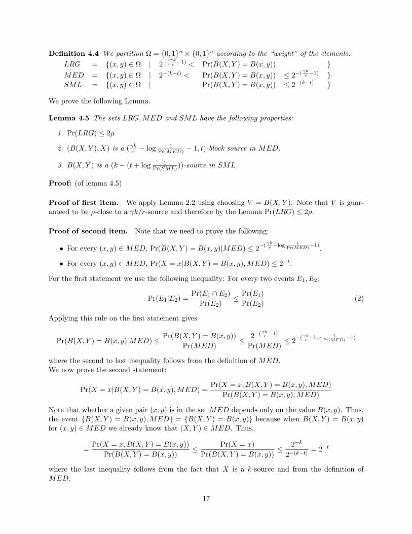
Definition 4.4 We partition Ω = 0, 1n × 0, 1u according to the “weight” of the elements.

LRG = (x, y) ∈ Ω | 2−( γkr−1) < Pr(B(X, Y ) = B(x, y))

MED = (x, y) ∈ Ω | 2−(k−t) < Pr(B(X, Y ) = B(x, y)) ≤ 2−( γkr−1)

SML = (x, y) ∈ Ω | Pr(B(X, Y ) = B(x, y)) ≤ 2−(k−t)

We prove the following Lemma.

Lemma 4.5 The sets LRG, MED and SML have the following properties:

1. Pr(LRG) ≤ 2ρ

2. (B(X, Y ), X) is a (γkr − log 1

Pr(MED) − 1, t)-block source in MED.

3. B(X, Y ) is a (k − (t + log 1Pr(SML)))-source in SML.

Proof: (of lemma 4.5)

Proof of first item. We apply Lemma 2.2 using choosing V = B(X, Y ). Note that V is guar-anteed to be ρ-close to a γk/r-source and therefore by the Lemma Pr(LRG) ≤ 2ρ.

Proof of second item. Note that we need to prove the following:

• For every (x, y) ∈ MED, Pr(B(X, Y ) = B(x, y)|MED) ≤ 2−( γk

r−log 1

Pr(MED)−1)

.

• For every (x, y) ∈ MED, Pr(X = x|B(X, Y ) = B(x, y), MED) ≤ 2−t.

For the first statement we use the following inequality: For every two events E1, E2:

Pr(E1|E2) =Pr(E1 ∩ E2)

Pr(E2)≤ Pr(E1)

Pr(E2)(2)

Applying this rule on the first statement gives

Pr(B(X, Y ) = B(x, y)|MED) ≤ Pr(B(X, Y ) = B(x, y))

Pr(MED)≤ 2−( γk

r−1)

Pr(MED)≤ 2

−( γkr−log 1

Pr(MED)−1)

where the second to last inequality follows from the definition of MED.We now prove the second statement:

Pr(X = x|B(X, Y ) = B(x, y), MED) =Pr(X = x, B(X, Y ) = B(x, y), MED)

Pr(B(X, Y ) = B(x, y), MED)

Note that whether a given pair (x, y) is in the set MED depends only on the value B(x, y). Thus,the event B(X, Y ) = B(x, y), MED = B(X, Y ) = B(x, y) because when B(X, Y ) = B(x, y)for (x, y) ∈ MED we already know that (X, Y ) ∈ MED. Thus,

=Pr(X = x, B(X, Y ) = B(x, y))

Pr(B(X, Y ) = B(x, y))≤ Pr(X = x)

Pr(B(X, Y ) = B(x, y))≤ 2−k

2−(k−t)= 2−t

where the last inequality follows from the fact that X is a k-source and from the definition ofMED.

17

Proof of the third item. Note that we need to prove that for (x, y) ∈ SML:

Pr(B(X, Y ) = B(x, y)|SML) ≤ 2−(k−(t+log 1

Pr(SML)))

The proof is similar to the proof of the first part in the second item. More precisely, we use therule (2) above. We argue that:

Pr(B(X, Y ) = B(x, y)|SML) ≤ Pr(B(X, Y ) = B(x, y)

Pr(SML)≤ 2−(k−t)

Pr(SML)≤ 2

−(k−(t+log 1Pr(SML)

))

2

We are now ready to prove Lemma 4.3.Proof: (of Lemma 4.3) We need to slightly change the partition above. The sets LRG, MED andSML are almost the partition we want. We only need to avoid a setup in which the sets MED orSML are too small, since in this case the effect of conditioning is too costly. Still, if one of the setsis very small we can safely add it to the “bad” elements and ignore it. This is the intuition behindthe following partition, which partitions 0, 1n × 0, 1u into three sets:

1. The set BAD will contain all (x, y) ∈ LRG. It will also contain all (x, y) ∈ SML ifPr(SML) < 2−t, and all (x, y) ∈ MED if Pr(MED) < 2−t.

2. The set BLK, (which corresponds to the set MED) contains all (x, y) ∈ MED if Pr(MED) ≥2−t. (Thus, BLK is empty if Pr(MED) < 2−t).

3. The set CON , (which corresponds to the set SML) contains all (x, y) ∈ SML if Pr(SML) ≥2−t. (Thus, BLK is empty if Pr(SML) < 2−t).

Lemma 4.3 follows from Lemma 4.5. 2

5 Constructing condensers

In this section we use a win-win analysis as outlined in Section 1.6 to construct a condenser. Themain Theorem of this Section is the following:

Theorem 5.1 For every n and k such that k ≥ 8 log5 n and 2 ≤ r ≤ log2 n there exist an explicit

(k, Ω(k/r), 1/ log2 n)-condenser Con : 0, 1n × 0, 1O(log(n/k)·log log n

log r+log n) → 0, 1

k log(n/k)r log r

It is helpful to consider two particular corollaries: For the first one we choose r = 2. This givesthat the condenser maintains a constant fraction of the initial randomness.

Corollary 5.2 For every n and k such that k ≥ 8 log5 n, there exists an explicit (k, Ω(k), 1/ log2 n)-condenser Con : 0, 1n × 0, 1O(log n

klog log n+log n) → 0, 1O(k log n

k).

For the second condenser we choose r = Θ(log n). This gives a condenser with seed O(log n) thatmaintains a (1/logn)-fraction of the initial randomness.

Corollary 5.3 For every n and k such that k ≥ 8 log5 n, there exists an explicit (k, Ω( klog n), 1/ log2 n)-

condenser Con : 0, 1n × 0, 1O(log n) → 0, 1 k2 .

In the remainder of this section we prove Theorem 5.1.

18

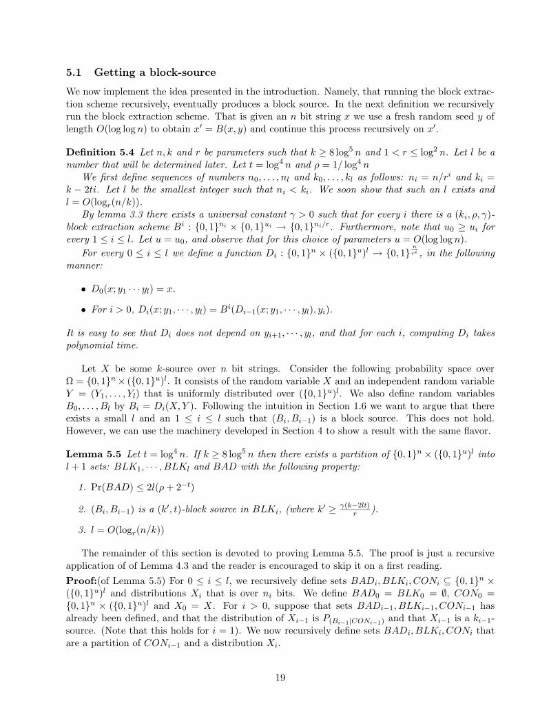
5.1 Getting a block-source

We now implement the idea presented in the introduction. Namely, that running the block extrac-tion scheme recursively, eventually produces a block source. In the next definition we recursivelyrun the block extraction scheme. That is given an n bit string x we use a fresh random seed y oflength O(log log n) to obtain x′ = B(x, y) and continue this process recursively on x′.

Definition 5.4 Let n, k and r be parameters such that k ≥ 8 log5 n and 1 < r ≤ log2 n. Let l be anumber that will be determined later. Let t = log4 n and ρ = 1/ log4 n

We first define sequences of numbers n0, . . . , nl and k0, . . . , kl as follows: ni = n/ri and ki =k − 2ti. Let l be the smallest integer such that ni < ki. We soon show that such an l exists andl = O(logr(n/k)).

By lemma 3.3 there exists a universal constant γ > 0 such that for every i there is a (ki, ρ, γ)-block extraction scheme Bi : 0, 1ni × 0, 1ui → 0, 1ni/r. Furthermore, note that u0 ≥ ui forevery 1 ≤ i ≤ l. Let u = u0, and observe that for this choice of parameters u = O(log log n).

For every 0 ≤ i ≤ l we define a function Di : 0, 1n × (0, 1u)l → 0, 1n

ri , in the followingmanner:

• D0(x; y1 · · · yl) = x.

• For i > 0, Di(x; y1, · · · , yl) = Bi(Di−1(x; y1, · · · , yl), yi).

It is easy to see that Di does not depend on yi+1, · · · , yl, and that for each i, computing Di takespolynomial time.

Let X be some k-source over n bit strings. Consider the following probability space overΩ = 0, 1n × (0, 1u)l. It consists of the random variable X and an independent random variableY = (Y1, . . . , Yl) that is uniformly distributed over (0, 1u)l. We also define random variablesB0, . . . , Bl by Bi = Di(X, Y ). Following the intuition in Section 1.6 we want to argue that thereexists a small l and an 1 ≤ i ≤ l such that (Bi, Bi−1) is a block source. This does not hold.However, we can use the machinery developed in Section 4 to show a result with the same flavor.

Lemma 5.5 Let t = log4 n. If k ≥ 8 log5 n then there exists a partition of 0, 1n × (0, 1u)l intol + 1 sets: BLK1, · · · , BLKl and BAD with the following property:

1. Pr(BAD) ≤ 2l(ρ + 2−t)

2. (Bi, Bi−1) is a (k′, t)-block source in BLKi, (where k′ ≥ γ(k−2lt)r ).

3. l = O(logr(n/k))

The remainder of this section is devoted to proving Lemma 5.5. The proof is just a recursiveapplication of of Lemma 4.3 and the reader is encouraged to skip it on a first reading.

Proof:(of Lemma 5.5) For 0 ≤ i ≤ l, we recursively define sets BADi, BLKi, CONi ⊆ 0, 1n ×(0, 1u)l and distributions Xi that is over ni bits. We define BAD0 = BLK0 = ∅, CON0 =0, 1n × (0, 1u)l and X0 = X. For i > 0, suppose that sets BADi−1, BLKi−1, CONi−1 hasalready been defined, and that the distribution of Xi−1 is P(Bi−1|CONi−1) and that Xi−1 is a ki−1-source. (Note that this holds for i = 1). We now recursively define sets BADi, BLKi, CONi thatare a partition of CONi−1 and a distribution Xi.

19

We first apply Lemma 4.3 on the i’th application of the block-extraction scheme B i on Xi−1

and Yi. It follows that 0, 1ni−1 × 0, 1u can be partitioned into three sets BAD, BLK, CON asin the lemma.

We “pull these events back to the original probability space”. That is we want to see these setsas a partition of CONi−1. More precisely, we define:

BADi = (x, y1, . . . , yl) ∈ CONi−1 : Di−1(x, y1, . . . , yl) ∈ BADBLKi = (x, y1, . . . , yl) ∈ CONi−1 : Di−1(x, y1, . . . , yl) ∈ BLKCONi = (x, y1, . . . , yl) ∈ CONi−1 : Di−1(x, y1, . . . , yl) ∈ CON

Note that this is a partition of CONi−1. Recall that Bi = Di(X, Y ) = Bi(Di−1(X, Y ), Yi). Thus,the distribution P(Bi|CONi) is exactly the same as P(Bi(Xi−1,Yi)|CON). Similarly P(Bi|BLKi) is exactlythe same as P(Bi(Xi−1,Yi)|BLK). We conclude that the guarantees of Lemma 4.3 give the following:

1. Pr(BADi) ≤ 2(ρ + 2−t)

2. (Bi, Bi−1) is a (γki−1

r − t, t)-block source in BLKi.

3. Bi is a ki-source in CONi.

We now define Xi to be the distribution P(Bi|CONi) that is over ni bits. Indeed, we have that Xi

is a ki-source. Thus, we can successfully define sets BADi, BLKi, CONi such that for each i > 0,these sets are a partition of CONi−1 and the three properties above hold.

We now show that at some step i, CONi = ∅. After i steps, the length of the i’th block isni = n/ri and ki = k−2it. Thus, after l = logr(4n/k) steps we have that the i’th block is of lengthat most k/4. At this point kl = k − 2lt ≥ k − 2 log5 n ≥ k/2. It follows that nl < kl and that thereis some i ≤ l for which CONi = ∅ as otherwise the third item above cannot hold (simply becauseit is impossible to have a distribution with more entropy than length).

We define: BAD = ∪1≤i≤lBADi. It follows that BLK1, . . . , BLKl and BAD are a partition ofΩ = 0, 1n × (0, 1l)u and the lemma follows. 2

5.2 Getting a condenser

In the previous section we showed how to get ` = O(logr(n/k) pairs of distributions such that (atleast in some sense) one of them is a block-source. Had we been able to construct a single blocksource, we could have used the block source extractor of corollary 2.6 to get an extractor. At thispoint however, we have many candidates (pairs Bi, Bi−1). We now run block source extractors onall pairs (using the same seed). It follows that one of the outputs is close to uniform and thereforethe concatenation of the outputs gives a condenser. We now formalize this intuition.

Construction 5.6 We use the parameters of Definition 5.4, namely: Let n, k and r be parameterssuch that k ≥ 8 log5 n and 1 < r ≤ log2 n. Let l = logr(4n/k), t = log4 n and ρ = 1/ log4 n. Letu = O(log log n) be the seed length for the block extraction scheme as determined in Definition 5.4.

Let k′ = γ(k−2lt)r

We define a function Con : 0, 1n × 0, 1ul+O(log n) → 0, 1n′where n′ is determined later.

Given inputs x ∈ 0, 1n and y ∈ 0, 1ul+O(log n), Con interprets its second argument as l stringsy1, · · · , yl ∈ 0, 1u and an additional string s of length O(log n). For 0 ≤ i ≤ l it computesbi = Di(x; y1, · · · , yl), (where Di is taken from definition 5.4), and oi = BE(bi, bi−1, s), (where BEis the block source extractor of corollary 2.6 using output length k′). The final output is (o1, · · · , ol),(which makes n′ = lk′).

20

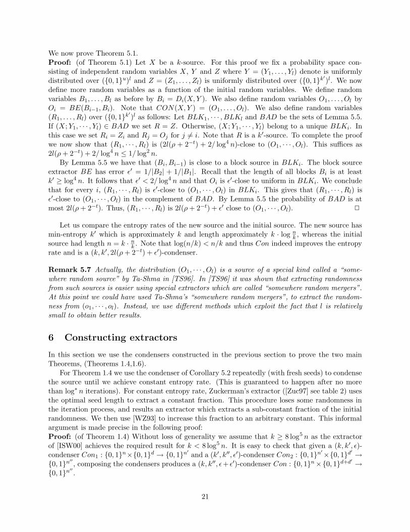
We now prove Theorem 5.1.Proof: (of Theorem 5.1) Let X be a k-source. For this proof we fix a probability space con-sisting of independent random variables X, Y and Z where Y = (Y1, . . . , Yl) denote is uniformlydistributed over (0, 1u)l and Z = (Z1, . . . , Zl) is uniformly distributed over (0, 1k′

)l. We nowdefine more random variables as a function of the initial random variables. We define randomvariables B1, . . . , Bl as before by Bi = Di(X, Y ). We also define random variables O1, . . . , Ol byOi = BE(Bi−1, Bi). Note that CON(X, Y ) = (O1, . . . , Ol). We also define random variables(R1, . . . , Rl) over (0, 1k′

)l as follows: Let BLK1, · · · , BLKl and BAD be the sets of Lemma 5.5.If (X; Y1, · · · , Yl) ∈ BAD we set R = Z. Otherwise, (X; Y1, · · · , Yl) belong to a unique BLKi. Inthis case we set Ri = Zi and Rj = Oj for j 6= i. Note that R is a k′-source. To complete the proofwe now show that (R1, · · · , Rl) is (2l(ρ + 2−t) + 2/ log4 n)-close to (O1, · · · , Ol). This suffices as2l(ρ + 2−t) + 2/ log4 n ≤ 1/ log2 n.

By Lemma 5.5 we have that (Bi, Bi−1) is close to a block source in BLKi. The block sourceextractor BE has error ε′ = 1/|B2| + 1/|B1|. Recall that the length of all blocks Bi is at leastk′ ≥ log4 n. It follows that ε′ < 2/ log4 n and that Oi is ε′-close to uniform in BLKi. We concludethat for every i, (R1, · · · , Rl) is ε′-close to (O1, · · · , Ol) in BLKi. This gives that (R1, · · · , Rl) isε′-close to (O1, · · · , Ol) in the complement of BAD. By Lemma 5.5 the probability of BAD is atmost 2l(ρ + 2−t). Thus, (R1, · · · , Rl) is 2l(ρ + 2−t) + ε′ close to (O1, · · · , Ol). 2

Let us compare the entropy rates of the new source and the initial source. The new source hasmin-entropy k′ which is approximately k and length approximately k · log n

k , whereas the initialsource had length n = k · n

k . Note that log(n/k) < n/k and thus Con indeed improves the entropyrate and is a (k, k′, 2l(ρ + 2−t) + ε′)-condenser.

Remark 5.7 Actually, the distribution (O1, · · · , Ol) is a source of a special kind called a “some-where random source” by Ta-Shma in [TS96]. In [TS96] it was shown that extracting randomnessfrom such sources is easier using special extractors which are called “somewhere random mergers”.At this point we could have used Ta-Shma’s “somewhere random mergers”, to extract the random-ness from (o1, · · · , ol). Instead, we use different methods which exploit the fact that l is relativelysmall to obtain better results.

6 Constructing extractors

In this section we use the condensers constructed in the previous section to prove the two mainTheorems, (Theorems 1.4,1.6).

For Theorem 1.4 we use the condenser of Corollary 5.2 repeatedly (with fresh seeds) to condensethe source until we achieve constant entropy rate. (This is guaranteed to happen after no morethan log∗ n iterations). For constant entropy rate, Zuckerman’s extractor ([Zuc97] see table 2) usesthe optimal seed length to extract a constant fraction. This procedure loses some randomness inthe iteration process, and results an extractor which extracts a sub-constant fraction of the initialrandomness. We then use [WZ93] to increase this fraction to an arbitrary constant. This informalargument is made precise in the following proof:Proof: (of Theorem 1.4) Without loss of generality we assume that k ≥ 8 log5 n as the extractorof [ISW00] achieves the required result for k < 8 log5 n. It is easy to check that given a (k, k′, ε)-condenser Con1 : 0, 1n×0, 1d → 0, 1n′

and a (k′, k′′, ε′)-condenser Con2 : 0, 1n′×0, 1d′ →0, 1n′′

, composing the condensers produces a (k, k′′, ε+ ε′)-condenser Con : 0, 1n ×0, 1d+d′ →0, 1n′′

.

21

Let us denote the entropy rate of a source by R(X) = k/n and let R′(X) = n/k = 1/R(X). Thecondenser of Corollary 5.2 produces a source X ′ that is close to a Ω(k) source over k log(n/k) bits.Thus, R(X ′) = Θ(1/ log(1/R(X))) or in other words, we have that R′(X ′) = Θ(log(R′(X)). Wenow apply the condenser recursively on X ′ using a fresh seed. After log∗ R′(X) ≤ log∗ n iterationsthe entropy rate becomes constant. Once the ratio is constant Zuckerman’s extractor ([Zuc97],see table 1), can be used to extract a constant fraction (say half) of the randomness using a freshseed of length O(log n) and error 1/ log2 n. Overall, we’ve used at most log∗ n iterations wherein each of them we required a seed of length at most O(log n · log log n) and the final applicationof Zuckerman’s extractor requires an additional O(log n) bits. Thus, the strategy described abovegives an extractor that uses seed length O(log n · log log n · log∗ n) bits. Recall that our condenserloses a constant fraction of the randomness in every iteration. Thus, after log∗ n iterations weextract only k/2O(log∗ n) random bits from the source, and produce an extractor which extracts a1/2O(log∗ n) fraction of the initial randomness. To get to a constant fraction we use the method ofWigderson and Zuckerman, [WZ93].10 Implementing the technique of Wigderson and Zuckermanmultiplies the seed and error by 2O(log∗ n). Thus, the total number of random bits is log n · log log n ·log∗ n · 2O(log∗ n) = O(log n · (log log n)2) as required. Furthermore the final extractor has errorsmaller than 1/ log n. 2

In the case of Theorem 1.6 we are shooting for the optimal seed length and cannot afford thecondenser of Corollary 5.2 or repeated condensing. Instead we use the condenser of Corollary 5.3interpreting it as a block extraction scheme. Viewed this way the condenser extracts a block B oflength k/2, therefore the distribution (B(X, Y ), X) forms a block source, since B is too short to“steal” all the randomness from X. (This intuition is formalized in the next Lemma). All that isleft is to use the block source extractor of corollary 2.6. The precise details follow.

Lemma 6.1 Let Con be the condenser of Corollary 5.3. If X is a k-source for k ≥ 8 log5 n thenthe distribution (Con(X, UO(log n)), X) is O(1/ log2 n)-close to an (Ω(k/ log n), log4 n)-block source.

Proof: Fix some n and k ≥ 8 log5 n, and let Con : 0, 1n × 0, 1u=O(log n) → 0, 1k/2 bethe (k, Ω(k/ log n), 1/ log2 n)-condenser of Corollary 5.3. For this proof we view Con as a block-extraction scheme B : 0, 1n×0, 1u → 0, 1n/r for r = 2n/k. It follows that B is a (k, ρ, γ)-blockextraction scheme for ρ = 1/ log2 n and γ = Ω(r/ log n). We remark that in particular γ 1.

We now consider the probability space of Section 4. The probability space is over the setΩ = 0, 1n × 0, 1u and consists of two independent random variables X (the given k-source)and Y that is uniformly distributed over 0, 1u. We set t = log4 n and apply Lemma 4.3 and letBAD, BLK, CON be the sets guaranteed by the lemma. We claim that CON = ∅.

This is because the Lemma guarantees that (B(X, Y ) is a (k − 2t)-source in CON . Note thatthe output length of B is k/2 whereas k − 2t > k/2 because k ≥ 8 log5 n. Thus, the Lemmasays that in CON , there is a random variable which has min-entropy larger than it length. Thisstatement can only be true if CON = ∅.

Lemma 4.3 also gives that:

• Pr(BAD) ≤ 2(ρ + 2−t)

• (B(X, Y ), X) is a (γkr − t, t)-block source in BLK.

10Wigderson and Zuckerman suggested to repeatedly extract randomness from the source, (using fresh seeds), untilone extracts the desired fraction. This gives that if m = k/p then m could be increased to (1 − α)k, (where α is anarbitrary constant), at the cost of multiplying d by O(p). (An exact formulation of the Wigderson and Zuckermantechnique can be found for example in [Nis96, NTS99]).

22

Thus, (B(X, Y ), X) is O(ρ+2−t)-close to a (γkr −t, t)-block source. Using again that k ≥ 8 log5 n,

we conclude that the distribution (Con(X, UO(log n)), X) is O(1/ log2 n)-close to an (Ω(k/ log n), log4 n)-block source as required. 2

We now prove Theorem 1.6.Proof: (of Theorem 1.6) As in the proof of Theorem 1.4 we can without loss of generality assumethat k ≥ 8 log5 n because the extractor of [ISW00] achieves the required result for k < 8 log5 n.Given a k-source, we use Lemma 6.1 to get a distribution that is close to a block-source and usethe block-source extractor of corollary 2.6. 2

7 Achieving small error

The statement of Theorems 1.4,1.6 is for constant error ε. The analysis provided in this papergives a slightly better result and allows to replace the requirement that ε be a constant withε = 1/(logn)c for any constant c. Still, our technique does not give good dependence of the seedlength on the error. We get better dependence on ε using the error reduction transformation of[RRV99], which transforms an extractor with large, (say constant) error into an extractor witharbitrary small error, while losing only a little bit in the other parameters. More precisely, afterundergoing the transformation, a factor of O(log m(log log m)O(1) + log(1/ε)) is added to d, andthe fraction extracted decreases by a constant. The latter loss makes no difference from our pointof view since we are only able to extract constant fractions. The first loss isn’t significant in thecase of Theorem 1.4, since the seed size is already larger than the optimal one by a multiplicativepolyloglog(n) factor. However, it completely spoils Theorem 1.6 and makes it inferior to Theorem1.4. Here is Theorem 1.4 rephrased using the error reduction transformation of [RRV99]:

Theorem 7.1 (Theorem 1.4 rephrased for non-constant ε) For every n, k and ε > exp( −n(log∗ n)O(log∗ n) ),

there are explicit (k, ε)-extractors Ext : 0, 1n × 0, 1O(log n·(log log n)O(1)+log(1/ε)) → 0, 1(1−α)k,where α > 0 is an arbitrary constant.

8 Transforming arbitrary extractors into strong extractors

It is sometimes helpful to have a stronger variant of extractors, called a strong extractor. A strongextractor is required to extract randomness “only from the source” and not “from the seed”.

Definition 8.1 A (k, ε)-extractor Ext : 0, 1n × 0, 1d → 0, 1m is strong if for every k-sourceX, the distribution (Ext(X, Ud) Ud) (obtained by concatenating the seed to the output of theextractor) is ε-close to a Um+d.

Intuitively, this is helpful since a strong extractor has the property that for any source a 1 − εfraction of the seeds extract randomness from that source. It is interesting to note that the conceptof strong-extractors preceded that of non-strong extractors, and the strong version was the onewhich was defined in the seminal paper of [NZ96]. Several extractors constructions, (with examplesbeing [TS96, ISW00] and the constructions of this paper) are non-strong or difficult to analyze asstrong.

The following Theorem shows that every non-strong extractor can be transformed into a strongone with essentially the same parameters.

23

Theorem 8.2 Any explicit (k, ε)-extractor Ext : 0, 1n × 0, 1d → 0, 1m can be transformedinto an explicit strong (k, O(

√ε))-extractor Ext′ : 0, 1n × 0, 1d+d′ → 0, 1m−(d+L+1) for d′ =

polylog(d/ε) and L = 2 log(1/ε) + O(1).

Let us consider the parameters of Ext′ compared to that of Ext. The seed length of Ext′ islonger than that of Ext by a factor that is only polylogarithmic (for large ε). The output length ofExt′ is shorter than that of Ext by d+L+1. The loss of d bits is unavoidable as the output of Extmay contain d bits of randomness from the seed. The additional loss of L + 1 bits can sometimesbe recovered (at the cost of increasing the seed length). Exact details are given in Remark 8.3.

Remark 8.3 In [RRV02] it was shown that any strong extractor which has seed length d andentropy-loss ∆ can be transformed into a strong extractor with seed length d+O(∆) and an optimalentropy loss of 2 log(1/ε) + O(1). Thus, if the initial extractor Ext had an entropy loss of ∆, wecan use our construction to get an extractor Ext′ with the parameters mentioned above, and thenuse [RRV02] to construct a strong extractor Ext′′ with seed length d′′ = d + d′ + O(∆) and optimalentropy loss. This addition is affordable if ∆ is small.

The intuition above also gives a hint for the construction. The output of Ext may contain dbits of randomness which “belong” to the seed. Still, it contains roughly m − d bits which do notdepend on the seed. Thus, fixing the seed, the output of Ext is a random source of length m whichcontains roughly m−d random bits. We can now use another extractor to extract this randomnessand “dismantle” the correlation between the seed and output. The extractor we need is one thatworks well when the source lacks only a very small amount of randomness. Such a constructionwas given by [GW97] and improved by [RVW00].

Theorem 8.4 [RVW00] There are explicit strong (k, ε)-extractors RV W : 0, 1n × 0, 1d′ →0, 1k−L For d′ = polylog((n − k)/ε) and L = 2 log(1/ε) + O(1).

Construction 8.5 Given a (k, ε)-extractor Ext : 0, 1n ×0, 1d → 0, 1m we construct Ext′ as

follows. Let RV W : 0, 1m × 0, 1d′=polylog(d/ε) → 0, 1m−d−1−L be an (m − d − 1, ε)-extractorguaranteed by Theorem 8.4. Then,

Ext′(x; (y, z)) = RV W (Ext(x, y), z)

The actual proof that Ext′ has the desired properties is slightly more complicated than theabove presentation. This is mainly because the above presentation ignores the error of Ext. Wenow give the formal proof.

Proof: (of Theorem 8.2) We now describe a probability space for this proof. It consists of threeindependent random variables: an arbitrary k-source X over n bit strings, a uniformly chosen stringY of length d and a uniformly chosen string Z of length d′.

Given strings x ∈ 0, 1n and y ∈ 0, 1d we define the weight of (x, y), denoted w(x, y) in thefollowing way:

w(x, y) = Pr(Ext(X, Y ) = Ext(x, y))

That is the weight of the string Ext(x, y) according to the distribution Ext(X, Y ). We say thata pair (x, y) is heavy if w(x, y) > 2−(m−1). We first claim that only few pairs are heavy.

Claim 1 Pr((X, Y ) are heavy) < 2ε.

24

Proof: Let V denote the distribution Ext(X, Y ). We now use Lemma 2.2. We have that V isε-close to an m-source (the uniform distribution). Therefore the probability under V of hitting anelement v such that PrV (V = v) > 2−(m−1) is bounded by 2ε and the claim follows. 2

Call a seed y ∈ 0, 1d bad if Pr((X, y) is heavy) >√

2ε. That is if for many choices of x, theoutput element is heavy. We now claim that there are few bad seeds.

Claim 2 The fraction of bad seeds is at most√

2ε.

Proof: The proof is a Markov argument. If the fraction of bad seeds were more than√

2ε thanPr((X, Y ) is heavy) > 2ε. 2

The following claim shows that running the extractor with a good seed produces a source whichlacks very few random bits.

Claim 3 For a good seed y, Ext(X, y) is√

2ε-close to an (m − d − 1)-source.

Proof: For a good y we know that Pr((X, y) is heavy) <√

2ε. That is at least a 1 −√

2ε fractionof the x’s have w(x, y) ≤ 2−(m−1)). For such an x,

Pr(Ext(X, y) = Ext(x, y)) = Pr(Ext(X, Y ) = Ext(x, y)|Y = y) ≤ w(x, y)

2−d≤ 2−(m−d−1)

2

We have that Ext′ runs RV W on the source Ext(X, Y ) using a fresh seed Z. Using the factthat for a good seed y, Ext(X, y) is close to a high entropy source we derive the following claim.

Claim 4 Given y ∈ 0, 1d, let Dy denote (Ext′(X; (y, Z))Z). For every good y, Dy is (2√

ε+ε)-close to uniform.

Proof: Note that Ext′(X; (y, Z)) = RV W (Ext(X, y), Z). The claim follows immediately fromclaim 3 and the fact that RV W is a strong extractor. 2

We now complete the proof of the theorem. Let D denote (EXT ′(X; (Y, Z)) Z). We need toshow that (DY ) is O(

√ε)-close to uniform. Note that D = DY (that is D is a convex combination

of the distributions Dy). As the fraction of bad seeds is at most O(√

ε) it is sufficient to show thatthat for any good seed y, (Dy Y ) is O(

√ε)-close to uniform. Note that as Y is independent of Dy

it is sufficient to show that Dy is O(√

ε)-close to uniform which follows from Claim 4. 2

9 Discussion

In a subsequent work [LRVW03] achieve extractors with better parameters than those constructedhere. Namely, for constant error ε > 0 they achieve a (k, ε)-extractor E : 0, 1n × 0, 1O(log n) →0, 1Ω(k) for every choice of k. Their construction uses some of the ideas of this paper (condensers,win-win analysis) as well as additional ideas.

The next milestone in extractor constructions seems to be achieving seed length d = O(log n)and output length m = k + d − O(1). (We remark that the difference between output length Ω(k)

25

and k is significant in some applications of extractors). This has already been achieved by [TSUZ01]for small values of k, (k = 2log n/ log log n) in a subsequent work.

Another important goal is to achieve the “correct dependance” of the seed length on ε for non-constant ε. Namely, to achieve an extractor with seed length d = O(log(n/ε)) and output length(say) m = Ω(k). We remark that both our approach and the approach of [LRVW03] do not givethis dependance.

10 Acknowledgments

We thank Russel Impagliazzo and Amnon Ta-Shma for helpful discussions, and particularly forbringing to our attention their insights on error correcting random sources. We are also grateful toanonymous referees for helpful comments.

References

[Blu86] M. Blum. Independent unbiased coin flips from a correlated biased source–A finite statemarkov chain. COMBINAT: Combinatorica, 6, 1986.

[CG89] B. Chor and O. Goldreich. On the power of two-point based sampling. Journal ofComplexity, 5(1):96–106, March 1989.

[CRVW02] M. R. Capalbo, O. Reingold, S. P. Vadhan, and A. Wigderson. Randomness conduc-tors and constant-degree lossless expanders. In Proceedings of the 34th Annual ACMSymposium on Theory of Computing, pages 659–668, 2002.

[GW97] O. Goldreich and A. Wigderson. Tiny families of functions with random properties: Aquality-size trade-off for hashing. RSA: Random Structures and Algorithms, 11, 1997.

[Imp99] R. Impagliazzo. private communication, 1999.

[ISW99] R. Impagliazzo, R. Shaltiel, and A. Wigderson. Near-optimal conversion of hardnessinto pseudo-randomness. In 40th Annual Symposium on Foundations of ComputerScience: October 17–19, 1999, New York City, New York,, pages 181–190, 1999.

[ISW00] R. Impagliazzo, R. Shaltiel, and A. Wigderson. Extractors and pseudo-random gen-erators with optimal seed length. In Proceedings of the thirty second annual ACMSymposium on Theory of Computing: Portland, Oregon, May 21–23, pages 1–10, 2000.

[Jus72] J. Justesen. A class of constructive asymptotically good algebraic codes. IEEE Trans.Info. Theory, 18:652–656, 1972.

[LRVW03] C. J. Lu, Omer Reingold, S. Vadhan, and A. Wigderson. Extractors: Optimal up toconstant factors. In Proceedings of the 35th Annual ACM Symposium on Theory ofComputing, New York, NY, USA, 2003. ACM Press.

[Nis96] N. Nisan. Extracting randomness: How and why: A survey. In Proceedings, EleventhAnnual IEEE Conference on Computational Complexity, pages 44–58, Philadelphia,Pennsylvania, 24–27 May 1996. IEEE Computer Society Press.

26

[NN93] J. Naor and M. Naor. Small-bias probability spaces: Efficient constructions and appli-cations. SIAM Journal on Computing, 22(4):838–856, August 1993.

[NTS99] N. Nisan and A. Ta-Shma. Extracting randomness: A survey and new constructions.JCSS: Journal of Computer and System Sciences, 58, 1999.

[NZ96] N. Nisan and D. Zuckerman. Randomness is linear in space. Journal of Computer andSystem Sciences, 52(1):43–52, February 1996.

[RR99] R. Raz and O. Reingold. On recycling the randomness of states in space boundedcomputation. In STOC: ACM Symposium on Theory of Computing (STOC), 1999.

[RRV99] R. Raz, O. Reingold, and S. Vadhan. Error reduction for extractors. In 40th AnnualSymposium on Foundations of Computer Science: October 17–19, 1999, New YorkCity, New York,, pages 191–201, 1999.

[RRV02] R. Raz, O. Reingold, and S. Vadhan. Extracting all the randomness and reducing theerror in trevisan’s extractors. JCSS: Journal of Computer and System Sciences, 65,2002.

[RSW00] O. Reingold, R. Shaltiel, and A. Wigderson. Extracting randomness via repeated con-densing. In Proceedings of the 41st Annual IEEE Symposium on Foundations of Com-puter Science, 2000.

[RTS00] J. Radhakrishnan and A. Ta-Shma. Bounds for dispersers, extractors, and depth-two superconcentrators. SIAM Journal on Discrete Mathematics, 13(1):2–24, February2000.

[RVW00] O. Reingold, S. Vadhan, and A. Wigderson. Entropy waves, the zig-zag graph prod-uct, and new constant-degree expanders and extractors. In IEEE, editor, 41st AnnualSymposium on Foundations of Computer Science: proceedings: 12–14 November, 2000,Redondo Beach, California, pages 3–13, 2000.

[Sha02] Ronen Shaltiel. Recent developments in extractors. Bulletin of the European Associa-tion for Theoretical Computer Science, 77, 2002.

[SU01] R. Shaltiel and C. Umans. Simple extractors for all min-entropies and a new pseudo-random generator. In 42nd IEEE Symposium on Foundations of Computer Science:proceedings: October 14–17, 2001, Las Vegas, Nevada, USA, pages 648–657, 2001.

[SV86] M. Santha and U. V. Vazirani. Generating quasi-random sequences from semi-randomsources. Journal of Computer and System Sciences, 33(1):75–87, April 1986.

[SZ98] A. Srinivasan and D. Zuckerman. Computing with very weak random sources. SICOMP:SIAM Journal on Computing, 28, 1998.

[Tre01] L. Trevisan. Extractors and pseudorandom generators. Journal of the ACM, 48(4):860–879, July 2001.

[TS96] A. Ta-Shma. On extracting randomness from weak random sources (extended ab-stract). In Proceedings of the Twenty-Eighth Annual ACM Symposium on the Theoryof Computing, pages 276–285, Philadelphia, Pennsylvania, 22–24 May 1996.

27

[TSUZ01] Amnon Ta-Shma, Christopher Umans, and David Zuckerman. Loss-less condensers,unbalanced expanders, and extractors. In Proceedings of the 33rd Annual ACM Sym-posium on Theory of Computing: Hersonissos, Crete, Greece, July 6–8, 2001, pages143–152, 2001.

[TSZS01] A. Ta-Shma, D. Zuckerman, and S. Safra. Extractors from Reed-Muller codes. InProceedings of the 42nd Annual IEEE Symposium on Foundations of Computer Science,pages 181–190, 1109 Spring Street, Suite 300, Silver Spring, MD 20910, USA, 2001.IEEE Computer Society Press.

[vN51] J. von Neumann. Various techniques used in connection with random digits. AppliedMath Series, 12:36–38, 1951.

[WZ93] A. Wigderson and D. Zuckerman. Expanders that beat the eigenvalue bound: Explicitconstruction and applications. In Proceedings of the Twenty-Fifth Annual ACM Sym-posium on the Theory of Computing, pages 245–251, San Diego, California, 16–18 May1993.

[Zuc90] D. Zuckerman. General weak random sources. In 31st Annual Symposium on Foun-dations of Computer Science, volume II, pages 534–543, St. Louis, Missouri, 22–24October 1990. IEEE.

[Zuc96] D. Zuckerman. Simulating BPP using a general weak random source. Algorithmica,16(4/5):367–391, October/November 1996.

[Zuc97] D. Zuckerman. Randomness-optimal oblivious sampling. Random Structures & Algo-rithms, 11(4):345–367, 1997.

28