In Proc. 13th IEEE International Conference on Computer Vision, Barcelona, Spain, November 2011.

Extracting Foreground Masks towards Object Recognition

Amir Rosenfeld and Daphna Weinshall

School of Computer Science and Engineering

Hebrew university of Jerusalem, Israel 91904

{rosenfld, daphna}@cs.huji.ac.il

Abstract

Effective segmentation prior to recognition has been

shown to improve recognition performance. However, most

segmentation algorithms adopt methods which are not ex-

plicitly linked to the goal of object recognition. Here we

solve a related but slightly different problem in order to as-

sist object recognition more directly - the extraction of a

foreground mask, which identifies the locations of objects in

the image. We propose a novel foreground/background seg-

mentation algorithm that attempts to segment the interest-

ing objects from the rest of the image, while maximizing an

objective function which is tightly related to object recog-

nition. We do this in a manner which requires no class-

specific knowledge of object categories, using a probabilis-

tic formulation which is derived from manually segmented

images. The model includes a geometric prior and an ap-

pearance prior, whose parameters are learnt on the fly from

images that are similar to the query image. We use graph-

cut based energy minimization to enforce spatial coherence

on the model’s output. The method is tested on the challeng-

ing VOC09 and VOC10 segmentation datasets, achieving

excellent results in providing a foreground mask. We also

provide comparisons to the recent segmentation method of

[7].

1. Introduction

Object recognition is one of the holy grails of computer

vision. While many current object recognition methods do

not rely on segmentation, a natural and common assump-

tion is that good segmentation prior to recognition can im-

prove the recognition results. This is because good segmen-

tation is expected to narrow down the number of options to

search among, allowing less room for false alarms and im-

proving the run-time. In addition, a well segmented object

will hopefully contain the relevant image features needed

for recognition, thus reducing the signal to noise ratio [18].

Following this assumption, a segmentation algorithm is

applied to the image, and the different segments are clas-

sified using a trained object classifier. The results may

vary according to how accurate the segmentation is, and of

course the quality of the classifier. However, the problem

is that many popular segmentation algorithms [19, 10, 17],

while having some desirable mathematical properties, have

little to do with the end goal, which is recognizing objects.

For instance, consider an image of a person’s face. For the

human observer, the person’s hairline is not perceived as

the boundary between the face and a different object. How-

ever, for an algorithm such as e.g. [10], the inter-segment

distance is large. In order for the segmentation algorithm to

keep the face and the hair in the same segment, the measure-

ment of the distance between them has to be small enough.

Thus, if segmentation was to achieve true object boundaries,

it would have to ignore these differences somehow.

Why indeed should one expect a segmentation algorithm

to identify true object boundaries? Most segmentation al-

gorithms (e.g., [3, 10, 17]) are designed to segment the en-

tire image with no regard to the notion of foreground or

background. While this may create a good delineation of

the boundaries of objects in the scene, the background be-

comes segmented as well. Thus we define a different goal

– to directly extract a foreground mask from the image

that indicates as accurately as possible where the objects

lie within the scene. This can serve as a first step for an

object recognition pipeline, without the additional noise of

an over-segmented background and with the advantage of

feeding the recognizer with relevant image regions.

In Section 3 we present a segregation algorithm that

achieves figure-ground segmentation, with the intent of

leaving the objects of interest whole and untouched. It

appears that in order to distinguish whole objects from

the background, one should have access to some implicit

knowledge about the objects of interest. Our approach at-

tempts to approximate this ideal situation, by training the

1

foreground/background segmentation algorithm using other

images similar to the query image, without using the class-

specific knowledge.

We present a probabilistic formulation comprised of two

components, corresponding to information about geometry

(shape & location) and appearance. The parameters of both

priors are estimated separately for each query image, us-

ing images from a large pre-segmented training set. The

geometric prior is estimated using the most similar images

according to the GIST representation [16], while the ap-

pearance prior is estimated using the most similar images

according to a Bag Of Words representation. In this way

we avoid the daunting task of learning the entire probabilis-

tic distribution of general foreground and background seg-

ments in images, relying instead on local approximations.

Segmentation is achieved by solving an energy minimiza-

tion problem over a superpixel graph attained using [1]. In

Section 4 we describe experiments on images from the PAS-

CAL 2009 and 2010 segmentation benchmarks, and offer a

way to compare our results to that of [7].

2. Related Work

As the complexity of images in which we attempt to rec-

ognize objects keeps increasing, simple methods such as

those based on Bag-of-Word features, which make a deci-

sion at an image level rather than object level, become less

effective. Thus, much recent work on object recognition

and multi-class labeling has focused on pre-segmenting the

image before applying the recognition algorithms.

It has been shown in [14] that good spatial support is im-

portant for object categorization. They compared the per-

formance of a classifier when presented with the visual fea-

tures of the bounding box surrounding the object vs. the

exact segmentation. For almost all object classes, exact

segmentation improves the categorization accuracy. They

used combinations of segments from over-segmented im-

ages using several popular segmentation methods, in order

to find an optimal cover for the objects in question. Given

the ground truth object boundary, the right combination of

segments which cover it is found quite easily, but of course

this information is not available for unseen images.

The work of [18] also shows how segmentation improves

the performance of standard recognition algorithms. They

first create a collection of segments by sampling the set

of stable segmentations [17] out of a much larger set, cre-

ated by varying the segmentation’s parameters and choosing

from among the results. The result is a “soup” of segments

- many possibly overlapping segments covering the image.

A baseline algorithm is applied to each of the resulting seg-

ments, thus ranking the segments according to classification

confidence. Largely overlapping segments are removed and

the top ranking ones are retained. While this segmentation

algorithm shows some impressive results, it has a very long

run time - many hours per image on a single computer, as

reported by the authors. In addition the cost function opti-

mized by the segmentation itself (i.e., stability of the seg-

mentation) is not related to object recognition.

In [3], hierarchical segmentation is created using the re-

sults of a generic contour detector as input, achieving very

good results. A different approach to ranking segments is

described in [7]. They create a very large (up to ten thou-

sands) set of segments and rank them based on a model

trained to predict their plausibility as object segments, given

a set of 34 regions and Gestalt properties.

ClassCut [2] automatically segments class objects, alter-

nating between segmenting object instances and learning a

class model. Their approach requires that the input set of

images contain only a single class of images. Avoiding the

question of perfect segmentation, [11] breaks the image into

super-pixels and trains a classifier to differentiate between

object classes based on the BOW representation of local

features extracted from each super-pixel and its neighbor-

hood. A CRF is employed to enforce spatial consistency

resulting in a multi-label segmentation.

Some papers use training images to gain knowledge

about the appearance of background and foreground. An

elegant approach is presented in [4], who employ both top-

down information (similar image fragments found in train-

ing images) and bottom up (image based) criteria to achieve

impressive results. However, their dataset includes rather

homogeneous (horse-side) images, while still requiring a

substantial amount of training examples. In [13] they use

multiple local and global image features types in a learning

framework, in order to detect salient object in images. They

train a CRF using these features, employing thousands of

training images.

In contrast to such methods, some of which require many

images for training, our approach is rather simple and uses

only a few (well selected) training examples for each test

image. Training is performed on the fly, requiring only a

few seconds to segment the image and provide the fore-

ground mask.

3. Approach

Given a set of manually segmented images, we wish to

learn a model which will allow us to segment a novel image

into two groups - foreground and background. The training

data consists of a set I1, I2, . . . , In of images. For each

image I we are given some ground-truth pixel-wise labeling

LI(x, y) for the objects in the image and their classes. The

original labels belong to a set of categories: LI(x, y) ∈C = {c1 · · · cm}, including a background category, which

is typically labeled implicitly (i.e., no label).

The labels provide much useful information for the task.

First, they provide the visual characteristics of foreground

objects. Second, we observe the scene containing the ob-

2

ject, making it possible to learn different segmentation rules

for different scenes. Lastly, we are given geometric cues

including shape and image location of foreground objects.

Next we show how all of those cues combine into a single

framework. Importantly, we do not use the label identity,

only the foreground-background distinction.

Similarly to [11] we formulate the problem as graph-

partitioning. Let G = (V,E) denote a graph whose nodes

correspond to superpixels. Those are obtained from [1], al-

lowing us to control both the approximate size of the graph

and its spatial regularity while still preserving object edges.

Neighboring superpixels define the graph’s edges.

Each node v ∈ V is first assigned a category label

L(v) ∈ C. Since we want to segment the image to fore-

ground and background segments as opposed to creating

class-specific labeling, we simplify this notation by using

an indicator function Fv , which takes the value of 1 iff L(v)is one of the foreground classes and 0 otherwise. Like L(v),Fv is well defined only if the superpixel contains exactly

one label. Using fine enough superpixels, this is almost al-

ways true. Note that under this definition, objects which are

adjacent in the image end up as one connected component

of the resulting foreground mask.

3.1. Probabilistic Formulation

Our model assigns to each node v ∈ V some probability

that it belongs to the foreground object given the underlying

superpixel Sv , P (Fv = 1 | Sv). It assigns to each pair of

neighboring nodes (u, v) ∈ E the probability that they have

the same label (i.e, both are from the foreground objects or

are background): P (Fu = Fv | Su, Sv). For brevity, we

write

Pf (v) = P (Fv = 1 | Sv) (1)

Ps(u, v) = P (Fu = Fv | Su, Sv) (2)

By doing so, we consider only two types of visual categories

- foreground and background, avoiding the additional com-

plexity of multi-class classification.

The two terms are combined to form the following en-

ergy function

− logP (F | G;α) =∑

v∈V

ηf (v) + α∑

(u,v)∈E

△s(u, v) (3)

where α is a regularization parameter, controlling the trade-

off between the fidelity and smoothing terms. We show how

to compute ηf (v) = − logPf (v) in Section 3.2.2. △s(u, v)is computed exactly as in [11], i.e.,

△s(u, v) = −logPs(u, v) = (L(Su, Sv)

1 + ‖Su − Sv‖) [Fi 6= Fj ]

(4)

(a) (b)

(c) (d) (e)

(f) (g) (h)

Figure 1. Automatic foreground extraction process: (a) Input im-

age. (c) Geometrically similar images, used to train the geometric

prior (f). (d) Visually similar images, used to train the appearance

prior (g). (e) SLIC [1] superpixels, used to aggregate the priors,

producing probability map (h). (b) Final foreground mask (green

tint) with ground-truth overlaid (red borders).

where L(Su, Sv) denotes the length of the boundary be-

tween Su and Sv , ‖Su − Sv‖ the norm of the color differ-

ence between superpixels in the LUV colorspace, and [·] the

indicator function.

3.2. Context on the fly

The probability distribution in (1) may in reality be quite

complex. In addition it is scene dependent, as a foreground

object in one scene may very well have the local appear-

ance properties of the background in another. We avoid

the daunting task of learning a model to represent the en-

tire distribution by simplifying the problem. Thus, for each

test image we consider only similar images observed in the

training set and use them to model the distribution. Our

probability distribution is composed of two semi indepen-

dent components: shape\location and local appearance. We

use different training sets to learn each component indepen-

dently.

3

3.2.1 Geometric Prior

In order to obtain a suitable training set to learn the geo-

metric prior, we use the GIST descriptor introduced in [16].

The descriptor gives low-dimensional representation of an

image used to find similar images in very large datasets with

good precision [8]. It sums up the response to different ori-

ented Gabor filters over a grid of rectangular areas over the

image, at multiple scales. The number of orientations may

differ per scale. The responses are concatenated into a sin-

gle feature vector. The standard implementation, used here,

produces a feature vector of length 960 for a color image.

We compute the descriptor for all images in the training

set. Given a test image I , we compute its GIST descriptor as

well, denoted G(I) ∈ RG. We find the KG-nearest neigh-

bors of this image from the set of training images, where

distances are measured using the GIST representation of

the images. Thus we retrieve a set of images whose gen-

eral layout is similar to that of the query image. Denote

those images by neiG(I) = {IN1 , . . . , INKG} (see example

in Fig. 1c).

The selected images are used to estimate a prior on the

distribution of locations of foreground objects by summing

over the foreground mask in each pixel (x, y):

PGf (x, y) =

1

KG

∑

INj∈neiG(I)

[LINj(x, y) ∈ foreground]

(5)

where LI(x, y) denotes the label of the image I at the coor-

dinates (x, y) after being normalized to the size of the test

image, and [·] denotes the indicator function. PGf (x, y) is

smoothed using a Gaussian kernel with σ = 7, to produce a

more continuous result. Thus we obtain a pixel-wise prob-

ability for the presence of a foreground object, see Fig. 1f.

Note that this prior is quite informative, since we sum

over the objects’ masks and not only their centers, thus gain-

ing information about the outline of the objects of interest.

We call this the geometric prior; examples are shown in

Fig. 2. The figure also shows the advantage of computing

this prior from Gist-based nearest neighbors, rather than us-

ing a generic mask computed from all the images in the

database (or a random sample of the images).

3.2.2 Appearance Prior

The GIST descriptor, while enabling the retrieval of scenes

with similar layout, typically retrieves images with different

scene content than the query image (see Fig. 2). Thus if we

wish to discriminate between foreground and background

on the basis of visual features, we need to choose a different

learning set. In order to find scenes with similar content,

we use a standard BOW method: a k-means dictionary is

computed for a large set of local descriptors from the set of

training images.

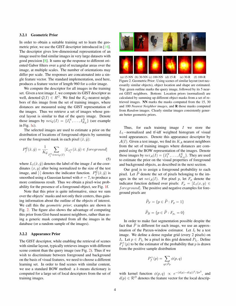
(a) 15-NN (b) 30-NN (c) 100-NN (d) 15-R (e) 30-R (f) 100-R

Figure 2. Geometric Prior: Using scenes of similar layout (not nec-

essarily similar objects), object location and shape are estimated.

Top: green outline marks the query image, followed by its 5 near-

est GIST neighbors. Bottom: Location priors (normalized) are

calculated by summing up different object masks from a set of re-

trieved images. NN marks the masks computed from the 15, 30

and 100 Nearest Neighbor images, and R those masks computed

from Random images. Clearly similar images consistently gener-

ate better geometric priors.

Thus, for each training image I we store the

L1−normalized and tf-idf weighted histogram of visual

word appearances. Denote this appearance descriptor by

A(I). Given a test image, we find its KA nearest neighbors

from the set of training images where distances are com-

puted using the BOW representation of the images. Denote

those images by neiA(I) = {IN1 , . . . , INKA

}. They are used

to estimate the prior on the visual properties of foreground

and background objects, as described in the next section.

Our goal is to assign a foreground probability to each

pixel. Let P denote the set of pixels belonging to the im-

ages in the set neiA(I). For pixel p, let Fp denote the

indicator function defined over pixels: Fp = [LI(x, y) ∈foreground]. The positive and negative examples for fore-

ground pixels are

PF = {p ∈ P : Fp = 1}

PB = {p ∈ P : Fpi= 0}

In order to make fast segmentation possible despite the

fact that P is different for each image, we use an approx-

imation of the Parzen-window estimator. Let It be a test

image. We define a dense regular grid (every 2 pixels) on

It. Let p ∈ PIt be a pixel in this grid denoted PIt . Define

P+f (p) to be the estimator of the probability that p is drawn

from the positive sample distribution

P+f (p) =

∑

q∈PF

φ(p, q)

with kernel function φ(p, q) ∝ e−(d(p)−d(q))2/2σ2

, and

d(p) ∈ RD denotes the feature vector for the local descrip-

4

tor at pixel p. Similarly

P−f (p) =

∑

q∈PB

φ(p, q)

The probability Pf (p) is thus calculated by the normal-

ized ratio:

Pf (p) =P+f (p)

P+f (p) + P−

f (p)(6)

This is done for each p ∈ PIt .

Since we use an exponential kernel function, the density

can be well approximated by considering only the k-nearest

neighbors of d(p) in the set of training examples. Although

nearest-neighbor algorithms are constantly improving [15],

it is still too time consuming if we want reasonable perfor-

mance: we need to perform |PIt | searches in the sample set

of size

∣∣∣P∣∣∣, which can be quite large (millions).

Instead, we create a quantized code-book (as in the bag-

of-features) model. Adapting the framework described in

[21], PHOW Descriptors are sampled at multiple scales and

locations from the training images. The descriptors are

quantized via K-means clustering. Each local descriptor in

both the test and training set is assigned its nearest cluster

in the K-means dictionary. Let wv ∈W = {w1, . . . , wk}denote the visual word assigned to the descriptor of pixel p.

The probability of foreground for the pixel p (Eq. (6)) is ap-

proximated by the probability for the corresponding visual

word wv:

Pf (wp) =

∑

q∈PF

[wq = wp]

∑

q∈PF

[wq = wp] +∑

q∈PB

[wq = wp](7)

In other words, we count how many times each visual word

is assigned the foreground or background labels.

This approximation allows us to quantize once the local

descriptors of each of the training and test images. Dur-

ing run-time, the density function (7) is estimated by count-

ing features from the corresponding images, which is very

quick and requires little memory. In the end, each pixel in

the grid p ∈ PIt is assigned a visual word wp and a proba-

bility Pf (wp).

3.3. Object­Edge Preserving Smoothing

In order to obtain the probabilities Pf (v), we aggregate

the local probabilities from both geometric prior (5) and ap-

pearance prior (7) using the superpixels as local decision

boundaries. Let Sv denote the set of pixels in the area of the

superpixel v, then

Pf (v) =1

|Sv|

∑

p∈Sv

Pf (wp)(PGf (x, y))

γ (8)

for wp the visual word assigned to the descriptor of pixel p,

and p = (x, y).The non-uniform smoothing resulting from the use of

super-pixels has the advantage of enhancing the effect of

Pf (wp) and PGf (x, y) inside objects and arbitrarily dispers-

ing the energy of those in more uniform image areas. This

is repeated for two levels of superpixel granularity - coarse

and fine. Coarse superpixels are used to estimate Pf (v) as

in Eq. (8). Then each image pixel in Sv is assigned the

probability Pf (v) and the process is repeated, only this time

computing Pf (v) over a more finely segmented image.

The coarse stage aggregates probabilities from relatively

large areas, thus potentially capturing more informative lo-

cal features at the cost of reduced accuracy. The fine super-

pixels allow for larger flexibility in the final segmentation

stage, since they are used as the graph nodes in the opti-

mization process, after Eqs. (7) and (4) are plugged into

Eq. (3). The energy is minimized using the graph-cut opti-

mization of [12, 11, 6, 5]. The parameter α is determined by

optimizing over a small portion (10%) of the dataset, and is

kept constant at 16 throughout the experiments. It can also

be chosen by cross-validation of the training data. The al-

gorithm is summarized in the box below.

4. Experiments

The algorithm was tested extensively on the Pascal

VOC09 and VOC10 datasets [9], which have many train-

ing images annotated with manual segmentation. We com-

puted local image descriptors on a dense regular grid (with

2-pixel spacing) using the color-PHOW implementation of

[21], which is computed at multiple scales. We summed up

the foreground prior estimated for each scale independently

with uniform weighting. The choice of descriptor was moti-

vated by the survey of [20]. The size of the visual dictionary

was set to K = 1000. We computed the GIST descrip-

tors on a 4x4 grid for all training images using a slightly

modified version of [16], allowing us to deal with rectan-

gular (rather than square) images. After the preprocessing

stage of extracting and quantizing dense local descriptors,

the runtime of the algorithm is 1-3 seconds on a PC with

8Gb of RAM and Intel core i5 CPU.

Examples can be seen in Fig. 3 and the suppl. material.

Clearly, the algorithm deals well with background clutter

and multiple connected components. The code will be made

available on the web.

4.1. Appearance vs. Geometry

To evaluate the contribution of the appearance and geo-

metric priors separately, we treat the problem as that of clas-

sification. Varying the threshold on the probability maps ob-

tained by using either the appearance prior or the geometric

prior alone (or their combination), we obtain a precision-

recall curve on the test dataset - see Fig. 4. Perhaps sur-

5

Algorithm 1 Extraction of Foreground Mask

1. GIt = (VIt , EIt)← the graph induced on It using coarse superpixels from ([1])

2. neiA(It)← {IN1 , . . . , INKA

}, the KA nearest BOW neighbors of A(It) in Itrain

3. Obtain PF , PB from P =⋃

H∈neiA(It)

{p : p ∈ PH}

4. For each word w ∈W calculate Pf (w) according to Eq. (7)

5. neiG(It)← {IN1 , . . . , INKG

}, the KG nearest GIST neighbors of G(It) in Itrain

6. Sum foreground masks from neiG(It) as in Eq. (5) to obtain PGf (x, y)

7. For each coarse superpixel v aggregate probabilities to obtain Pf (v) as in (8); split results into finer superpixels

8. Optimize − logP (F | G;α) from Eq. (3) via graph-cut to obtain the foreground mask F(I)

Figure 3. Some of our segmentation results on VOC09 and VOC10. The algorithm provides a foreground mask (green tint) with the goal to

extract all foreground objects (red outline), without oversegmenting the background. All results were obtained using the same parameters

of KA = KG = 30 along with the geometric prior. The foreground need not be a single connected component (1st row, right). The

algorithm succeeds in highly cluttered backgrounds (2nd row, right & center). See supp. material for many more examples.

prisingly geometry alone is a stronger cue than local ap-

pearance. Arguably, this happens because most objects are

approximately centered in the PASCAL benchmarks. How-

ever, the learning process also contributes to this success; as

can be seen in Fig. 2, both location and shape are captured

more concisely when using good training examples.

4.2. Quality of Segmentation

4.2.1 Overlap score

Since our algorithm provides a foreground mask (sometime

with several connected components), we score each result

produced by our algorithm according to its overlap score:

O =|S ∩ S′|

|S ∪ S′|

where S is the ground-truth foreground mask, i.e., the union

of all object segments, and S′ is the result of our algo-

rithm. This scoring scheme reflects the fact that our algo-

rithm makes no effort to split adjacent foreground objects.

Instead, it aims to produce foreground masks that include

all objects in the image. The average of this score over the

test set of the VOC09 benchmark is given in Table 1.

6

0 0.2 0.4 0.6 0.8 10

0.2

0.4

0.6

0.8

1

Recall

Pre

cis

ion

visual

visualXgeom

geom

vis−spXgeom

visual − rand

geom − rand

Figure 4. Performance comparison of appearance and geometrical

priors. Geometry alone (solid green) is stronger than local ap-

pearance cues (solid blue). Superpixel aggregation (black) further

enhances the result, for all but low-recall cases. Dashed green/blue

lines show the performance drop when choosing random images

for learning instead of those chosen by our method.

Dataset CPMC Ours Ours-Mask

VOC09 0.4018 0.4263 0.4708

VOC10 - 0.4107 0.4570Table 1. Comparison of our method’s overlap score to CPMC [7],

using their first ranked segmentation. In the column under “Ours-

Mask” we give the modified score, where image adjacent object

segments in the ground-truth are merged into one connected com-

ponent.

To study the effect of the algorithm’s parameters KG and

KA, we varied them and calculated the overlap score over

the test set. We tested how switching on and off the use of

geometric prior changed the final results. Summary of this

test can be seen in Fig. 5. Clearly the use of the geometric

prior isn’t always the right choice, as can be seen by the

mean grade attained by choosing for each image its best

scoring method. To illustrate, Fig. 6 shows a case where

using the geometric prior hinders the result.

4.2.2 Comparison to Segmentation

The following score, used in [7], measures the covering of

the ground-truth segmentation by a machine segmentation:

C(S, S′) =1

N

∑

R∈S

|R| ∗maxR′

O(R,R′)

where N denotes the number of pixels in the image, |R| the

number of pixels in the ground truth segment, and O the

overlap.

1 2 3 4 5 10 15 30 50 100 all (750)0.1

0.2

0.3

0.4

0.5

0.6

no. neighbors

avg

. o

ve

rla

p s

co

re

visual

visual X geom

best

Figure 5. Mean segment overlap score on VOC09 for varying num-

bers of nearest neighbors chosen for learning geometric & appear-

ance priors (KA = KG). Dashed red lines (“visual”) - perfor-

mance using the appearance prior only. Green (“visual x geom”) -

contribution of the geometric prior. The solid blue curve (“best”)

shows performance when choosing for each image its best scoring

method.

(a) (b)

Figure 6. Geometric prior doesn’t always help. (a) Segmentation

using appearance & geometric prior. (b) Segmentation using ap-

pearance only.

We compare our results to those of [7], which achieves

excellent segmentation results by creating diverse seg-

mentations and ranking them automatically using a learnt

model. Having produced multiple segmentations, they com-

pute the average of the best covering score for varying num-

ber of segments, chosen according to their ranking.

The mean covering score we obtain for a single segmen-

tation using KA = KG = 30 is 0.4263. On average this is

slightly better when compared to the score obtained by the

first ranking segment of [7], which is 0.4018. With addi-

tional segments (which our method does not produce), their

method achieves higher accuracies than ours. We note that

the runtime of [7] is approx. 3 minutes, as compared to 1-3

seconds of our own method; this is because their algorithm

solves the more complicated problem of full segmentation,

and does so many times.

Since our algorithm aims at creating whole foreground

masks, it is at a disadvantage when the scoring method ex-

7

pects it to split connected foreground blobs into different

segments, as was done in the comparison above. A more

suitable score should regard connected foreground objects

as the same ground-truth segment. Under this relaxation,

we achieve a much higher result of 0.4708. The results

are summarized in Table 1, where results on VOC10 are

reported as well.

5. Discussion & Conclusions

We have presented an efficient and effective algorithm

for foreground/background segmentation, motivated by ob-

ject recognition perspective. The algorithm learns both ge-

ometric and appearance priors for the task. For each prior,

a different set of training images is chosen independently,

in order to maximize the relevant data in the training set.

This choice allows for learning from limited datasets, as

images whose content and layout are both similar to the

query image may be rare. It leads to a powerful representa-

tion that seems to discriminate foreground from background

quite well. We note that although the ground-truth annota-

tions of the dataset contain rich class-specific information

on multiple classes, none of this information is used by our

algorithm, none but the distinction between background and

foreground. The algorithm was tested on two challenging

datasets, Pascal VOC09 and VOC10.

To assist object recognition, the foreground mask com-

puted by our algorithm can be fed into any choice of recog-

nition algorithm. New features may be subsequently com-

puted more robustly from the foreground area only, before

attempting final recognition.

References

[1] R. Achanta, A. Shaji, K. Smith, A. Lucchi, P. Fua, and

S. Susstrunk. SLIC Superpixels. Technical report, EPFL,

2010. 2, 3, 6

[2] B. Alexe, T. Deselaers, and V. Ferrari. Classcut for unsu-

pervised class segmentation. Computer Vision–ECCV 2010,

pages 380–393, 2010. 2

[3] P. Arbelaez, M. Maire, C. Fowlkes, and J. Malik. From con-

tours to regions: An empirical evaluation. 2009. 1, 2

[4] E. Borenstein. Combining top-down and bottom-up segmen-

tation. In Proceedings IEEE workshop on Perceptual Orga-

nization in Computer Vision, CVPR, 2004. 2

[5] Y. Boykov and V. Kolmogorov. An experimental comparison

of min-cut/max-flow algorithms for energy minimization in

vision. IEEE transactions on Pattern Analysis and Machine

Intelligence, 26(9):1124–1137, September 2004. 5

[6] Y. Boykov, O. Veksler, and R. Zabih. Efficient approxi-

mate energy minimization via graph cuts. IEEE transactions

on Pattern Analysis and Machine Intelligence, 20(12):1222–

1239, November 2001. 5

[7] J. Carreira and C. Sminchisescu. Constrained parametric

min-cuts for automatic object segmentation. In Computer

Vision and Pattern Recognition (CVPR), 2010 IEEE Confer-

ence on, pages 3241–3248. IEEE, 2010. 1, 2, 7

[8] M. Douze, H. Jegou, H. Sandhawalia, L. Amsaleg, and

C. Schmid. Evaluation of gist descriptors for web-scale im-

age search. In Proceeding of the ACM International Confer-

ence on Image and Video Retrieval, pages 1–8. ACM, 2009.

4

[9] M. Everingham, L. Van Gool, C. Williams, J. Winn,

and A. Zisserman. The PASCAL visual object classes

(VOC) challenge. International journal of computer vision,

88(2):303–338, 2010. 5

[10] P. F. Felzenszwalb and D. P. Huttenlocher. Efficient Graph-

Based Image Segmentation. International Journal of Com-

puter Vision, 59(2):167–181, Sept. 2004. 1

[11] B. Fulkerson, A. Vedaldi, and S. Soatto. Class segmentation

and object localization with superpixel neighborhoods. In

Proceedings of the International Conference on Computer

Vision, October 2009. 2, 3, 5

[12] V. Kolmogorov and R. Zabih. What energy functions can

be minimized via graph cuts? IEEE transactions on Pattern

Analysis and Machine Intelligence, 26(2):147–159, February

2004. 5

[13] T. Liu, Z. Yuan, J. Sun, J. Wang, N. Zheng, X. Tang, and

H. Shum. Learning to detect a salient object. Published by

the IEEE Computer Society, 2010. 2

[14] T. Malisiewicz and A. Efros. Improving spatial support for

objects via multiple segmentations. 2, 2007. 2

[15] M. Muja and D. G. Lowe. Fast approximate nearest neigh-

bors with automatic algorithm configuration. In Interna-

tional Conference on Computer Vision Theory and Applica-

tion VISSAPP’09), pages 331–340. INSTICC Press, 2009. 5

[16] A. Oliva and A. Torralba. Modeling the shape of the scene: A

holistic representation of the spatial envelope. International

Journal of Computer Vision, 42(3):145–175, 2001. 2, 4, 5

[17] A. Rabinovich, T. Lange, J. Buhmann, S. Belongie, and

E. Zurich. Model order selection and cue combination for

image segmentation. CVPR (1), pages 1130–1137, 2006. 1,

2

[18] A. Rabinovich, A. Vedaldi, and S. Belongie. Does image

segmentation improve object categorization. 1, 2

[19] J. Shi and J. Malik. Normalized Cuts and Image Segmenta-

tion. Analysis, 22(8):888–905, 2000. 1

[20] K. E. A. van de Sande, T. Gevers, and C. G. M. Snoek.

Evaluating color descriptors for object and scene recogni-

tion. IEEE Transactions on Pattern Analysis and Machine

Intelligence, 32(9):1582–1596, 2010. 5

[21] A. Vedaldi and B. Fulkerson. VLFeat: An open and portable

library of computer vision algorithms. http://www.

vlfeat.org/, 2008. 5

8