Extra-precise Iterative Refinement for Overdetermined Least

Squares Problems∗

James Demmel† Yozo Hida‡ Xiaoye S. Li§ E. Jason Riedy¶

May 28, 2008

Abstract

We present the algorithm, error bounds, and numerical results for extra-precise iterativerefinement applied to overdetermined linear least squares (LLS) problems. We apply our lin-ear system refinement algorithm to Bjorck’s augmented linear system formulation of an LLSproblem. Our algorithm reduces the forward normwise and componentwise errors to O(εw),where εw is the working precision, unless the system is too ill conditioned. In contrast to linearsystems, we provide two separate error bounds for the solution x and the residual r. The refine-ment algorithm requires only limited use of extra precision and adds only O(mn) work to theO(mn2) cost of QR factorization for problems of size m-by-n. The extra precision calculation isfacilitated by the new extended-precision BLAS standard in a portable way, and the refinementalgorithm will be included in a future release of LAPACK and can be extended to the othertypes of least squares problems.

1 Background

This article presents the algorithm, error bounds, and numerical results of the extra-precise iterativerefinement for overdetermined least squares problem (LLS):

minx‖b−Ax‖2 , (1)

where A is of size m-by-n, and m ≥ n.The xGELS routine currently in LAPACK solves this problem using a QR factorization. There

is no iterative refinement routine. We propose to add two routines: xGELS_X (expert driver) andxGELS_RFSX (iterative refinement). In most cases, users should not call xGELS_RFSX directly.∗This research was supported in part by the NSF Grant Nos. CCF-0444486, EIA-0122599, and CNS-0325873;

the DOE Grant Nos. DE-FC02-01ER25478 and DE-FC02-06ER25786. The third author was supported in part bythe Director, Office of Advanced Scientific Computing Research of the U.S. Department of Energy under contractDE-AC03-76SF00098. The authors wish to acknowledge the contribution from Intel Corporation, Hewlett-PackardCorporation, IBM Corporation, and the NSF EIA-0303575 in making hardware and software available for the CITRISCluster which was used in producing these research results.†demmel@cs.berkeley.edu, Computer Science Division and Mathematics Dept., University of California, Berkeley,

CA 94720.‡yozo@cs.berkeley.edu, Computer Science Division, University of California, Berkeley, CA 94720.§xsli@lbl.gov, Computational Research Division, Lawrence Berkeley National Laboratory, Berkeley, CA 94720.¶ejr@cs.berkeley.edu, Computer Science Division, University of California, Berkeley, CA 94720.

1

Our first goal is to obtain accurate solutions for all systems up to a condition number thresholdof O(1/εw) with asymptotically less work than finding the initial solution, where εw is the workingprecision. To this end, we first compute the QR factorization and obtain the initial solutionin hardware-supported fast arithmetic (e.g., single or double precisions). We refine the initialsolution with selective use of extra precision. The extra-precise calculations may use slower softwarearithmetic, e.g. double-double [2] when working precision already is double. Our second goal is toprovide reliable error bounds for the solution vector x as well as the residual vector r.

As we will show, we can provide dependable error estimates and small errors for both x andresidual r = b − Ax whenever the problems are acceptably conditioned. In this paper the phraseacceptably conditioned will mean the appropriate condition number is no larger than the thresholdcond thresh = 1

10·max{10,√m+n}·εw

, and ill conditioned will mean the condition number is larger thanthis threshold. If the problem is ill conditioned, either because the matrix itself is nearly singularor because the vector x or r is ill conditioned (which can occur even if A is acceptably conditioned),then we cannot provide any guarantees. Furthermore, we can reliably identify whether the problemis acceptably conditioned for the error bounds to be both small and trustworthy. We achieve thesegoals by first formulating the LLS problem as an equivalent linear system [5], then applying ourlinear system iterative refinement techniques that we developed previously [8].

We make the following remarks regarding the scope of this paper. Firstly, we describe thealgorithms and present the numerical results only for real matrices here. But the algorithms can beextended to complex matrices straightforwardly, as we already did for the linear systems refinementprocedure. Secondly, we assume A has full column rank, and the QR factorization does not involvecolumn pivoting, although column pivoting could be easily incorporated into the algorithm. Inthe rank-deficient cases, we recommend using the other LAPACK routines that perform QR withcolumn pivoting (xGELSY) or SVD (xGELSS or xGELSD). SVD is the most reliable method to solvethe low rank LLS problem, but the development of the companion iterative refinement algorithmis still an open problem.

2 Extra-precise Iterative Refinement

In this section, we present the equivalent linear system formulation for the LLS problem, and weadapt a linear system iterative refinement procedure to refine the solution of the LLS problem.

2.1 Linear system formulation

Let r = b− Ax be the residual, the LLS problem is equivalent to solving the following augmentedlinear system of dimension m+ n [3, 6]:(

Im AAT 0

)(rx

)=(b0

). (2)

Then, we can apply our extra-precise iterative refinement algorithm [8] to linear system (2) toobtain more accurate vectors x and r. Algorithm 1 shows a high-level sketch of the refinementprocedure.

We monitor the progress of both the solution vector x and the residual vector r to provide smallinfinity-norm relative normwise and componentwise errors (unless the system is too ill conditioned).

2

Here, the QR factorization of A and the solution for the updates in Step (2) are carried out inworking precision εw. By “doubled arithmetic” we mean the precision used is twice the workingprecision, which we denote as εd. In our numerical experiments, we use IEEE-754 single precisionas the working precision (εw = 2−24) and IEEE-754 double precision in our residual calculations(εd = 2−53). All the extra-precise calculations are encapsulated in the eXtended precision BLASlibrary (XBLAS) [15]. In the XBLAS routines, the input/output arguments are stored in theworking precision, the same as the standard BLAS routines. The extra-precise accumulation isperformed only internally.

Note that the extra precision εd we use in this paper satisfies εd ≤ ε2w. The algorithm willstill improve accuracy if εd is in between ε2w and εw, except that some parameters in our stoppingcriteria need to be adjusted, and the accuracy results will be weaker accordingly. That is, theclaim that the errors can be reduced to O(εw) for acceptably conditioned problems would bebased on a cond thresh smaller than 1

10·max{10,√m+n}·εw

. Future work remains to perform numericalexperiments to quantify the effect.

Algorithm 1Obtain the first solution x(1) using QR factorization of A,

and compute the first LLS residual r(1) = b−Ax(1).Repeat

(1) Compute the residual vectors s(i) and t(i): (may be in doubled arithmetic)s(i) = b− r(i) −Ax(i)

t(i) = −AT r(i)(2) Solve for the corrections dr(i) and dx(i) using the existing QR factorization A:(

Im AAT 0

)(dr(i)

dx(i)

)=(s(i)

t(i)

)(3) Update the solution vectors: (may be in doubled arithmetic)

r(i+1) = r(i) + dr(i)

x(i+1) = x(i) + dx(i)

i = i+ 1Until r(i) and/or x(i) “accurate enough”

2.2 Extra precision

Our extra-precise iterative refinement algorithm not only computes the residual in extended preci-sion but also may carry the solution vector [r;x] in doubled precision. Therefore, in Step (1), thefirst residual is computed as

s(i) = b− (r(i) + r(i)t )−A(x(i) + x

(i)t ) , (3)

where rt and xt are used to store the “tails” of each floating point component of r and x.We have extended the XBLAS with a new routine to compute this portion of the residual. The

existing XBLAS routine xGEMV2_X sufficies to compute the other portion, t(i) = AT (r(i) + r(i)t ).

3

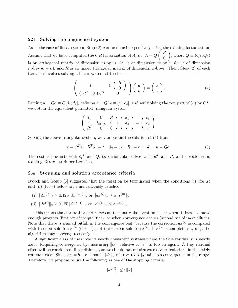
2.3 Solving the augmented system

As in the case of linear system, Step (2) can be done inexpensively using the existing factorization.

Assume that we have computed the QR factorization of A, i.e, A = Q

(R0

), where Q ≡ (Q1, Q2)

is an orthogonal matrix of dimension m-by-m, Q1 is of dimension m-by-n, Q2 is of dimensionm-by-(m − n), and R is an upper triangular matrix of dimension n-by-n. Then, Step (2) of eachiteration involves solving a linear system of the form Im Q

(R0

)(RT 0

)QT 0

( uv

)=(st

). (4)

Letting u = Qd ≡ Q[d1; d2], defining c = QT s ≡ [c1; c2], and multiplying the top part of (4) by QT ,we obtain the equivalent permuted triangular system In 0 R

0 Im−n 0RT 0 0

d1

d2

v

=

c1c2t

.

Solving the above triangular system, we can obtain the solution of (4) from

c = QT s, RTd1 = t, d2 = c2, Rv = c1 − d1, u = Qd . (5)

The cost is products with QT and Q, two triangular solves with RT and R, and a vector-sum,totaling O(mn) work per iteration.

2.4 Stopping and solution acceptance criteria

Bjorck and Golub [6] suggested that the iteration be terminated when the conditions (i) (for x)and (ii) (for r) below are simultaneously satisfied:

(i) ‖dx(i)‖2 ≥ 0.125‖dx(i−1)‖2 or ‖dx(i)‖2 ≤ ε‖x(0)‖2(ii) ‖dr(i)‖2 ≥ 0.125‖dr(i−1)‖2 or ‖dr(i)‖2 ≤ ε‖r(0)‖2

This means that for both x and r, we can terminate the iteration either when it does not makeenough progress (first set of inequalities), or when convergence occurs (second set of inequalities).Note that there is a small pitfall in the convergence test, because the correction dx(i) is comparedwith the first solution x(0) (or r(0)), not the current solution x(i). If x(0) is completely wrong, thealgorithm may converge too early.

A significant class of uses involve nearly consistent systems where the true residual r is nearlyzero. Requiring convergence by measuring ‖dr‖ relative to ‖r‖ is too stringent. A tiny residualoften will be considered ill conditioned, so we should not require excessive calculations in this fairlycommon case. Since Ax = b− r, a small ‖dr‖2 relative to ‖b‖2 indicates convergence in the range.Therefore, we propose to use the following as one of the stopping criteria:

‖dr(i)‖ ≤ ε‖b‖

4

Our algorithm attempts to achieve small errors for both r and x, and in both normwise andcomponentwise measures. In other words, for those users who do want r as accurately as possible,we will also try to compute r with a small componentwise error. We will use the following quantitiesin stopping criteria:

• For normwise error, we will scale r by 1/‖b‖∞, and x by 1/‖x‖∞.

• For componentwise error, we will scale each ri by 1/|ri|, and each xi by 1/|xi|.We use two state variables x-state and r-state (∈ {working, converged, no-progress}) to track

normwise convergence status for x and r, and two other state variables xc-state and rc-state (∈{unstable, working, converged, no-progress}) to track componentwise convergence status for x andr. Fig. 1 depicts the state transition diagrams for both normwise (Fig. 1(a)) and componentwise(Fig. 1(b)) convergence statuses.

The normwise state variable x-state (or r-state) is initialized to be in working state. The stateof x is changed to converged when the correction dx(i+1) is too small to change the solution xi

much (condition dx x def= ‖dx(i+1)‖/‖xi‖ ≤ ε). When convergence slows down sufficiently (conditiondxrat

def= ‖dx(i+1)‖/‖dx(i)‖ > ρthresh), the state is changed from working to no-progress. The iterationmay continue because the other state variables are still making progress, thus, the no-progress statemay change back to working state when convergence becomes faster again (condition dxrat ≤ρthresh).

The componentwise state variable xc-state (or rc-state) is initialized to be in unstable state,meaning that each component of the solution has not settled down for convergence testing. Whenall the components are settled down (condition dxc(i+1) def= maxj |dx(i+1)

j /xij | ≤ cthresh), the state ischanged from unstable to working. cthresh is the threshold below which the solution is consideredstable enough for testing the componentwise convergence, and dxcrat

def= dxc(i+1)/dxc(i). The restof the state transitions follow the rules similar to those of the normwise case.

Finally, we terminate the refinement iteration when all four state variables (x-state, r-state,xc-state, and rc-state) are no longer in working state, or when an iteration count threshold isreached. Thus, we are simultaneously testing four sets of stopping criteria—as long as at least oneof the four state variables is in working state, we continue iterating.

Once the algorithm has terminated, we evaluate the conditioning of each solution in both norm-and componentwise senses. If the solution is acceptably conditioned and the algorithm terminatedin the converged state for that norm, we accept the result as accurate. Otherwise we reject thesolution. Our current implementation returns an error estimate of 1.0 to signify rejected solutions.Table 1 summarizes our acceptance criteria.

In the numerical experiments presented in Section 4, we use ρthresh = 0.5 and cthresh = 0.25,which we recommend to be the default settings in the code. Note that a larger ρthresh (aggressivesetting) allows the algorithm to make progress more slowly and take more steps to converge, whichmay be useful for extremely difficult problems.

In contrast to linear systems, here we separate the augmented solution into two parts, x and r.If both converge, the algorithm should behave the same as for linear systems [8]. On the other hand,we may have half of the solution (say x) converge while the other half (r) stops making progress.Or it may be the case that half is ill conditioned while the other half is not. We will providecondition analysis of this “two-parts” approach in Section 3, and show empirically in Section 4 thatthe augmented systems for LLS are harder than the usual linear systems because r resides in thedata space while x resides in the solution space, and they may be of different scales.

5

Accepted Rejectedcondition estimate ≥ cond thresh Xsolution & norm not converged Xconverged and cond. est. < cond thresh X

Table 1: Summary of conditions where a particular solution and norm are accepted as accurate.cond thresh = 1

10·max{10,√m+n}·εw

.

WORKING NO_PROGRESS

CONVERGED

dx_x <= ε

dxrat > rho_thresh

dxrat <= rho_thresh

dxrat <= rho _thresh

(a) x-state (or r-state) transition

WORKING NO_PROGRESS

CONVERGED

UNSTABLE

dxc <= ε

dxc <= c_threshdxcrat <= rho_thresh dxcrat > rho_thresh

dxcrat <= rho_thresh

(b) xc-state (or rc-state) transition

Figure 1: State transition diagrams. ρthresh is the threshold on the ratio of successive corrections,above which the convergence is considered too slow. (a) normwise, and (b) componentwise.

2.5 Scaling

In the case of linear systems, we typically perform row and/or column equilibrations to avoidover/underflows and to reduce the condition number of scaled A. We now discuss scaling for theLLS problems.

The driver routine xGELS_X first uses a simple scaling before solving the LLS problem. Itindependently scales A by α and b by β up or down to make sure their norms are in the range[SMLNUM, 1/SMLNUM], where SMLNUM ≈ UNDERFLOW/εw. The LLS problem we solve becomes

miny‖β · b− α ·Ay‖2 = min

y‖β(b−A(α/β · y)‖2 = min

y‖b−A(α/β · y)‖2 ≡ min

x‖b−Ax‖2 ,

where x = α/β · y. In addition, xLARFG, which computes a single Householder reflection, does verycareful scaling if necessary, and depends on xNRM2 to not over/underflow.

The analysis of the linear system iterative refinement suggests that the convergence rate of the

refinement procedure depends on the condition number of the augmented matrix B =(Im AAT 0

).

Bjorck suggested using a non-zero scalar α to scale the LLS problem as in b−Ax⇒ (b−Ax)/α [3].This does not change the computed LLS solution, but now the augmented system involves the

matrix Bα =(αIm AAT 0

). It was shown by Bjorck that the eigenvalues of Bα are

λ(Bα) ={

α2 ± (α

2

4 + σ2i )

1/2

α

6

where σi, i = 1, . . . , n are the singular values of A. In particular, if we choose α = σmin/√

2, the

condition number κ2(Bα) takes the minimum value, κ2(Bα) = 12 +

√14 + 2 κ2

A ≤ 2κ2(A), whichshould lead to fastest convergence of the refinement for the augmented system. However, whencarefully working through the iteration in Algorithm 1 and the solve procedure (5), we see thatonly the quantities related to r (i.e., t(i), dr(i), and r(i)) are scaled by 1/α; the other quantitiesremain the same. Thus, as long as α is chosen to be a power of the radix, the computed solutionand the rounding errors are not changed, Although Bα has a lower condition number, it does notmatter for our algorithm. We have confirmed this from numerical experiments. From the analysisin Section 3 we will see that κ(Bα) does not play any role in the conditioning of the LLS problem.

Now, we discuss general equilibrations. We cannot row equilibrate A in our framework as thiswould change its range and the norm we are minimizing. We can potentially column equilibrate Aby a general diagonal matrix D, which means scaling x by D−1. As long as we pick the entries in Dto be powers of the radix, we would not introduce any rounding errors (modulo over/underflows).The normwise convergence criteria for x would be affected, because ‖dx‖, ‖x‖, and ‖dx(i+1)/‖dx(i)‖will be different for unscaled or scaled x. With O(n) work, we can compute these quantitiescorresponding to the unscaled x, and use them in the stopping criteria, just as we did for linearsystems [8]. It remains our future work to see how this type of scaling affects the convergence rate.

3 Normwise and Componentwise Condition Numbers

The refinement algorithm can return various error bounds for the solutions x and r. In order todetermine when our error bounds are reliable, we need condition numbers for both x and r.

Applying the standard componentwise perturbation analysis to (2), we assume that the com-puted solutions r = r + δr and x = x+ δx satisfy the equations(

Im A+ δA(A+ δA)T 0

)(rx

)=(b+ δb

0

), (6)

where |δA| ≤ ε|A|, and |δb| ≤ ε|b|. This is equivalent to the perturbed normal equation

(A+ δA)T (A+ δA)x = (A+ δA)T (b+ δb).

Since ATAx = AT b, subtracting it from the above equation and noting that r = b+δb− (A+δA)x,we get

δx = A+(δb− δA · x) + (ATA)−1δAT · r , (7)

where A+ = (ATA)−1AT . Using the inequalities |δA| ≤ ε|A| and |δb| ≤ ε|b|, we obtain the followingbound on each component of δx

|δx| ≤ ε [|A+| (|b|+ |A| · |x|) + |(ATA)−1| · |AT | · |r|] .Taking norms, we get

‖δx‖∞‖x‖∞ ≤ ε‖|A

+|(|b|+ |A| · |x|)‖∞ +∥∥|(ATA)−1| · |AT | · |r|∥∥∞

‖x‖∞ .

7

Therefore, the following can be used as a normwise condition number for x:

κxnormdef=‖|A+|(|b|+ |A| · |x|)‖∞ +

∥∥|(ATA)−1| · |AT | · |r|∥∥∞‖x‖∞ . (8)

Note that this derivation is valid assuming that A + δA has full rank, i.e., κ2(A) ≡ ‖A‖2‖A+‖2 isnot too large. In Section 4.2, we will confirm this assumption in practice.

In the case of linear systems, the basic solution method (GEPP) and the iterative refinementalgorithm are column scaling invariant. Therefore, we may choose the column scale factors suchthat each component of the scaled solution is of magnitude about one; thus, the usual normwiseerror bound measures the componentwise error as well.

We would like to apply the same technique to the augmented linear system (2). Letting Dr ≈diag(r), and Dx ≈ diag(x), our refinement iterations can be thought of as solving the followingscaled system (

Im AAT 0

)(Dr

Dx

)(zrzx

)=(b0

)(9)

where zr = D−1r r ≈ 1, and zx = D−1

x x ≈ 1. The same solution method for the augmented systemcan be used, but the convergence of zr and zx are monitored simultaneously as with r and x.

Applying the analogous perturbation analysis to (9), we assume that the computed solutionszr = zr + δzr and zx = zx + δzx satisfy the equations(

Im A+ δA(A+ δA)T 0

)(Dr

Dx

)(zrzx

)=(b+ δb

0

). (10)

By the same algebraic manipulation, we obtain an expression for δzx that is simply the expres-sion for δx (7) with a pre-factor D−1

x . That is,

δzx = D−1x

[A+(δb− δAx) + (ATA)−1δAT r

]Taking norms, we get

‖δzx‖∞ ≤ ε(∥∥|D−1

x ||A+|(|b|+ |A| · |x|)∥∥∞ +∥∥|D−1

x | · |(ATA)−1| · |AT | · |r|∥∥∞) (11)

Since zx ≈ 1, ‖δzx‖∞ ≈ maxi|δzx|i|zx|i = maxi

|D−1x δx|i|D−1x x|i

= maxi|δx|i|x|i . Therefore, (11) measures the

componentwise error of x, and the following can be used as the componentwise condition number:

κxcompdef=∥∥|D−1

x | · |A+|(|b|+ |A| · |x|)∥∥∞ +∥∥|D−1

x | · |(ATA)−1| · |AT | · |r|∥∥∞ . (12)

We can use LAPACK’s condition estimator (SLACON, based on Hager-Higham’s algorithm [11])to estimate each norm in (12). For example, let d = |b| + |A||x|, D = diag(d) > 0, and e be thevector of all ones; then,∥∥|D−1

x | · |A+|(|b|+ |A| · |x|)∥∥∞ =∥∥|D−1

x | · |A+| d∥∥∞ =∥∥|D−1

x | · |A+|De∥∥∞ =∥∥|D−1

x | · |A+|D∥∥∞=

∥∥|D−1x A+D|∥∥∞ =

∥∥D−1x A+D

∥∥∞

The condition estimator requires multiplying D−1x A+D and (D−1

x A+D)T with some vectors,which involves triangular solves using R if we have A = QR at hand.

Similarly, let d = |AT | · |r|, D = diag(d) > 0; then,∥∥|D−1x | · |(ATA)−1| · |AT | · |r|∥∥∞ =

∥∥|D−1x | · |(ATA)−1|D∥∥∞ =

∥∥D−1x (ATA)−1D

∥∥∞ ,

which can be estimated analogously.

8

We now derive the condition numbers for r. Consider the first set of equations in (6):

r + δr = b+ δb− (A+ δA)x .

Subtracting r = b− Ax from the above equation, we have δr = δb− δAx− Aδx. Substituting (7)for δx, we obtain

δr = δb− δAx− (AA+(δb− δAx) +A(ATA)−1δAT r)

= (Im −AA+)(δb− δAx)− (A+)T δAT r (13)

Then, the bounds for each component of δr and δzr are given by

|δr| ≤ ε [|Im −AA+| (|b|+ |A| · |x|) + |(A+)T | · |AT | · |r|] ,|δzr| ≤ ε|D−1

r |[|Im −AA+|(|b|+ |A| · |x|) + |(A+)T | · |AT | · |r|] .

Thus, the normwise condition number for r can be defined as

κrnormdef=‖ |Im −AA+| (|b|+ |A| · |x|) ‖∞ +

∥∥|(A+)T | · |AT | · |r|∥∥∞‖b‖∞ . (14)

The componentwise condition number for r can be defined as

κrcomp =∥∥|D−1

r | · |Im −AA+|(|b|+ |A| · |x|)∥∥∞ +∥∥|D−1

r | · |(A+)T | · |AT | · |r|∥∥∞ . (15)

Observe that, given A = (Q1, Q2)(R0

)= Q1R, we have Im − AA+ = Im − Q1Q

T1 . Since

‖Im −Q1QT1 ‖2 = min{1,m− n}, we expect the effect of multiplication by |Im −AA+| to be small,

and so we can use the following approximate but cheaper-to-compute formula as the normwisecondition number for r:

κrnorm cheapdef=‖ |b|+ |A| · |x| ‖∞ +

∥∥|(A+)T | · |AT | · |r|∥∥∞‖b‖∞ . (16)

By the same token, the following cheap formula could be considered as the componentwisecondition number for r:

κrcomp cheap =∥∥|D−1

r | · (|b|+ |A| · |x|)∥∥∞ +

∥∥|D−1r | · |(A+)T | · |AT | · |r|∥∥∞ . (17)

Again, Hager-Higham’s algorithm can be used to estimate the respective norms∥∥|(A+)T | · |AT | · |r|∥∥∞ and∥∥|D−1

r | · |(A+)T | · |AT | · |r|∥∥∞.Examining Eq. (12) for κxcomp, we notice that the second term can be proportional to κ(A)2,

depending on the size of residual r. That is, when the LLS problem is compatible or nearly so(with small r), the second term is negligible, and the sensitivity of x to perturbation is similar tothe case of linear system. When the angle between b and Ax is large (with large r), or closer toπ/2, the solution x would have small components, which are much more sensitive to perturbation.

Fig. 3 compares the condition numbers estimated from formulae (14)–(17). There are altogetherone million randomly generated test matrices of size 100× 50 (see Section 4.1 for tests generation).

9

log10 κrnorm cheap

log 1

0κ

r norm

Regular vs. cheap condition estimates: R normwise

0.0% 0.4%

0.2%

99.2%

0.2%

0 2 4 6 8 10 12 14100

101

102

103

104

105

0

2

4

6

8

10

12

14

(a) normwise

log10 κrcomp cheap

log 1

0κ

r com

p

Regular vs. cheap condition estimates: R componentwise

4.2% 48.3%

0.0%

47.5%

0 5 10 15100

101

102

103

104

0

5

10

15

(b) componentwise

Figure 2: Comparison between regular and cheap condition estimations for R.

Fig. 2(a) shows that in normwise measure, the two estimates given by (14) and (16) are very close—they agree to within a factor four, with the cheaper ones yielding slightly smaller values. Therefore,it is safe for our code to use (16). On the other hand, in the componentwise measure (see Fig. 2(b)),the cheap estimation given by (17) can be much smaller than the one given by (15)—sometimesover 400x smaller. This is because if Dr has highly varying entries, leaving out the |Im − AA+|factor could make the estimation arbitrarily small. In this case, we shall use the more expensiveformula (15).

Table 2 summarizes the estimated condition numbers and error bounds to be returned from thenew LAPACK routine. Here,

• γ is a constant factor used for setting a threshold to differentiate the acceptably conditionedproblems from the ill conditioned ones. Based on our empirical results from the linear systemrefinement, a good value of γ is max{10,

√m+ n} [8].

• εw is the machine epsilon in working precision.

• ρmax is the maximum ratio of successive corrections, which is a conservative estimate of therate of convergence. For example, ρxmax

def= maxj≤i‖dx(j+1)‖∞‖dx(j)‖∞

. Similarly, ρmax is defined forthe componentwise case.

The code also returns a componentwise backward error BERR(r, x) = max(ω1, ω2) [5, pp. 36],where

ω1 = max1≤i≤m

|r +Ax− b|i(|r|+ |A||x|+ |b|)i , ω2 = max

1≤i≤n

|AT r|i(|A|T |r|)i .

4 Numerical Experiments

We now present numerical results from our iterative refinement algorithm. All the test runs wereconducted on the CITRIS Itanium-2 Cluster at UC Berkeley.1 Each node has dual 1.3 GHz Itanium

1http://www.millennium.berkeley.edu/citris/

10

Condition number Relative error Error estimate

x norm. κxnorm (8) Exnorm = ‖x−x‖∞‖x‖∞ Bxnorm = max

{‖dx(i+1)‖∞/‖xi‖∞

1−ρxmax

, γεw

}comp. κxcomp (12) Excomp = maxk

∣∣∣ x(k)−x(k)x(k)

∣∣∣ Bxcomp = max{‖Dxdx

i‖∞1−ρx

max, γεw

}r norm. κrnorm (16) Ernorm = ‖r−r‖∞

‖b‖∞ Brnorm = max{‖dr(i+1)‖∞/‖bi‖∞

1−ρrmax

, γεw

}comp. κrcomp (15) Ercomp = maxk

∣∣∣ r(k)−r(k)r(k)

∣∣∣ Brcomp = max{‖Drdr

i‖∞1−ρr

max, γεw

}Table 2: Summary of condition numbers and error estimates, where Dx = diag(x) and Dr =diag(r). The error estimates are derived from the analysis of the geometric-decreasing sequence oferrors from iterations, see [8].

2 (Madison) processors. The operating system is Linux 2.6.18, and the compilers and flags areifort -no-ftz -fno-alias -funroll-loops -O3 for Fortran code, and icc -O3 for C code.

We use single precision εw = 2−24 ≈ 6 × 10−8 as working precision and double precisionεd = 2−53 ≈ 10−16 in the refinement. Running in single precision allows us to test the inputspace more thoroughly. Also, we can rely on the well-tested double precision codes to producetrustworthy true solutions. The iteration control parameters ρthresh and cthresh are set to 0.5 and0.25, respectively. Recall that γ = max{10,

√m+ n}. We will analyze in detail the results of one

million least squares problems of dimension 100× 50.Recall that we would like to achieve the following two goals from the refinement procedure:

Goal 1 For acceptably conditioned problems, we obtain small errors.

Goal 2 A small error bound returned from the code is trustworthy.

We will demonstrate that we meet these goals with the following data:

• norm- and componentwise relative errors in x (Section 4.2.1), where the errors are ≤ γ · εwwhenever the specific condition number ≤ 1

10 γ εw;

• error estimates for x (Section 4.2.2), where the error estimates are within a factor of 10 ofthe true error whenever the specific condition number ≤ 1

10 γ εw;

• norm- and componentwise relative errors in r (Section 4.3.1), similar to x;

• error estimates for r (Section 4.3.2), similar to x; and

• iteration counts (Section 4.4), where the median number of iterations for acceptably condi-tioned systems is two.

4.1 Test problem generation

We need to generate many test cases with a wide range of condition numbers, and the right-handsides b having angles ranging from close to zero to close to π/2 with respect to the column span ofA. We now describe our procedure for generating the test problems.

• Generate matrix A.

11

1. Randomly pick a condition number κ with log2 κ distributed uniformly in [0, 24]. Thiswill be the (2-norm) condition number of the matrix before any scaling is applied. Therange chosen will generate both easy and hard problems (since εw = 2−24).

2. Pick a set of singular values σi’s from one of the following choices:

(a) One large singular value: σ1 = 1, σ2 = · · · = σn = κ−1.(b) One small singular value: σ1 = σ2 = · · · = σn−1 = 1, σn = κ−1.

(c) Geometrical distribution: σi = κ−i−1n−1 for i = 1, 2, . . . , n.

(d) Arithmetic distribution: σi = 1− i−1n−1(1− κ−1) for i = 1, 2, . . . , n.

3. Pick k randomly from {3, n/2, n}. Move the largest and the smallest singular values(picked in step 1) into the first k values, and let Σ be the resulting diagonal matrix. Let

A = UΣ(V1

V2

), (18)

where U , V1, and V2 are random orthogonal matrices with dimensions n, k, and n −k, respectively. If κ is large, this makes the leading k columns of A nearly linearlydependent. U , V1 and V2 are applied via sequences of random reflections of dimensions2 through n, k or n− k, respectively.

• Generate vector b.

1. Compute b1 = Ax (with random x) using double-double precision but rounded to singleprecision in the end (using the XBLAS routine BLAS_sgemm_x). Normalize b1 such that‖b1‖2 = 1.

2. Compute A = QR. Pick vector d of m random real numbers uniformly distributed in(−1, 1). Compute b2 = d − QQTd, and normalize b2 such that ‖b2‖2 = 1. Now b2 isorthogonal to the columns of A.

3. Pick a random θ ∈ [0, π/2] as follows. First set θ = π · 2u, where u is uniformlydistributed in [−26,−1]. Then, with probability 0.5, flip θ = π/2 − θ. Compute finalb = cos θ · b1 + sin θ · b2.

Note that steps 2 and 3 are carried out in double precision. The final b is then rounded tosingle precision.

• Compute xtrue and rtrue by solving the augmented linear equations (2) using double precisionlinear system solver with double-double precision iteration refinement (the new LAPACKroutine DGESVXX).

Using the above procedure, we have systematically generated one million test problems ofdimension 100 × 50. Among them, the condition numbers of A range between 1.0 and 4.9 × 108,and the condition numbers of the scaled augmented matrix Bα (see Section 2.5) range between 57.8and 8.1× 109. Fig. 3 shows the 2D histograms of the properties of the test problems: the angle θbetween b and the column span of A, and the conditioning of A. In the 2D histogram, each shadedsquare at coordinate (x, y) indicates the population of the problems that have θ ∈ [10x, 10x+1/4] andcondition number κ∞(A) ∈ [10y, 10y+1/4]. Fig. 3(a) plots against θ, while Fig. 3(b) plots against

12

log10 θ

log 1

0κ(A

)Matrix statistics: 1000000

-6 -4 -2 0100

101

102

103

104

1

2

3

4

5

6

7

8

(a) θ

log10(π2 − θ)

log 1

0κ(A

)

Matrix statistics: 1000000

-6 -4 -2 0100

101

102

103

104

1

2

3

4

5

6

7

8

(b) π2− θ

Figure 3: Statistics of the one million test problems.

π/2− θ. These plots show that we indeed have a good sampling of easy and hard problems, havingmany cases with θ close to 0 and many cases with θ close to π/2. In fact, we sample the regionaround tiny and near-π/2 angles much more than the “easier” middle region. They also show thatour method generated angles arbitrarily close to zero, but not arbitrarily close to π/2.

These types of 2D histogram plots will be used in the remainder of the paper to illustrate allthe test results.

4.2 Results for x

Of the one million test problems, 577,412 are acceptably conditioned in normwise measure (i.e.,κxnorm < 1

10 γ εw), and 355,330 are acceptably conditioned in componentwise measure (i.e., κxcomp <

110 γ εw

).

4.2.1 True error

First, in Fig. 4, we plot the normwise true error of x obtained from single precision QR factor-ization without iterative refinement (the LAPACK routine SGELS). As shown, the error growsproportionally with the condition number of x, κxnorm. The horizontal solid line is at the valueExnorm = γεw ≈ 7.3 · 10−7. A matrix below this line indicates that the true error is of or-der εw, which is the most desirable convergence case. We also plot this solid line in the otheranalogous figures for all the errors (e.g., Excomp, E

rnorm, and Ercomp) and the error bounds (e.g.,

Bxnorm, B

xcomp, B

rnorm, and Br

comp). The vertical solid line (also in the other analogous figures) is atthe value κxnorm = 1

10 γ εw≈ 1.4 · 105, which separates the acceptably conditioned problems from

the ill conditioned ones. In addition, we often plot a dashed line at the value of εw as a referenceline. In each quadrant defined by the horizontal and vertical cutoff lines, we label the number oftest problems falling in that quadrant.

Fig. 5 shows the results of normwise true error of x after our refinement procedure terminates,whether the code reports convergence or not. Regarding κxnorm, there are 577,412 acceptablyconditioned problems that appear in the left two quadrants. Among them, 577,377 converged, and

13

log10 κxnorm

log 1

0E

x norm

Before refnement

433091 422588

144321

0 5 10 15100

101

102

103

104

-8

-6

-4

-2

0

Figure 4: Before refinement: true error of x vs.κxnorm.

log10 κxnorm

log 1

0E

x norm

Normwise error vs. condition number κxnorm.

35 110538

577377 312050

0 5 10 15100

101

102

103

104

-9

-8

-7

-6

-5

-4

-3

-2

-1

0

1

Figure 5: After Refinement: true error of x vs.κxnorm (all cases).

log10 κxnorm

log 1

0κ∞

(A)

Condition estimates: A vs. x

1.1% 2.6%

11.1%

15.7%

41.0% 28.5%

0 5 10 15100

101

102

103

104

0

2

4

6

8

10

12

14

Figure 6: κ∞(A) vs. κxnorm.

log10 κxnorm

log 1

0E

x norm

Normwise error vs. condition number κxnorm.

74665

577376 302322

0 5 10 15100

101

102

103

104

-8

-6

-4

-2

0

Figure 7: Normwise error of x vs. κxnorm (con-verged cases).

35 have errors larger than our error threshold. For those 35 problems, the condition number ofA (κ∞(A) def= ‖A‖∞‖A+‖∞) is larger than or close to the condition threshold; thus they are closeto rank deficient. Fig. 6 compares the condition number of A vs. the condition number of x. Asshown, many problems have κ∞(A) larger than κxnorm.

In the situation when A is nearly rank deficient, our computed κxnorm may not be trustworthyfor two reasons: 1) our perturbation analysis for Eq. (8) assumes that A is not too ill conditioned,and 2) κxnorm depends on the computed x and r, which are not accurate. Therefore, these problemsshould also be characterized as ill conditioned. In fact, with closer examination of those 35 cases,we found that all of them did not converge. Our code only accepts the results when the iterationconverges w.r.t. the corresponding state variable. When it does not converge, we simply set theerror estimate to one. In Fig. 7, we make another histogram plot that filters out the unconvergedcases. That is, we show only the problems with x-state = converged (see Section 2.4). Now, noneof the problems appears in the upper left quadrant.

Fig. 8 shows the results of componentwise true error of x versus condition number. There are

14

355,330 acceptably conditioned problems. Without refinement (Fig. 8(a)), the error grows propor-tionally with the condition number. After refinement (Fig. 8(b)), all the acceptably conditionedproblems converged. Among the remaining very ill conditioned ones, 449,483 of them still con-verged. Overall, only 19.5% (195,187 out of one million) of the problems did not converge. Fig. 9plots only the cases that have converged.

log10 κxcomp

log 1

0E

x com

p

Before refinement

353065 644670

2265

0 5 10 15100

101

102

103

104

-9

-8

-7

-6

-5

-4

-3

-2

-1

0

1

(a) before refinement

log10 κxcomp

log 1

0E

x com

p

Componentwise error vs. condition number κxcomp.

195187

355330 449483

0 5 10 15100

101

102

103

104

-9

-8

-7

-6

-5

-4

-3

-2

-1

0

1

(b) after refinement

Figure 8: Componentwise error of x vs. condition number (all cases).

From Figs. 7 and 9 we draw the most important conclusion that for all the acceptably con-ditioned and converged problems, our algorithm delivers tiny errors for x, both normwise andcomponentwise. That is, Goal 1 is clearly achieved for the solution x. Moreover, the algorithmconverged with small errors for a large fraction of the ill conditioned problems, that is, 73.8% of the422,588 problems with κxnorm ≥ 1

10 γ εw, and 69.7% of the 644,670 problems with κxcomp ≥ 1

10 γ εw.

4.2.2 Reliability of error bounds

From the user’s point of view, a small error can be recognized only from a small error boundestimated from the algorithm. Figs. 10 and 11 show the relation between the true errors and theerror bounds (see Table 2). In these plots, the diagonal line marks where the true error equals theerror bound. A matrix above the diagonal corresponds to an overestimate, and a matrix below thediagonal corresponds to an underestimate.

For the acceptably conditioned (measured in κxnorm and κxcomp, respectively) and convergedproblems (Figs. 10(a) and 10(b)), the algorithm converged to a solution with error of at most1.1 ·10−7, and returned an error bound γεw ≈ 7.3 ·10−7, which never underestimates the true error.

For the ill conditioned problems (Figs. 11(a) and 11(b)), a large fraction of the problems stillconverged and the error bounds reflect small errors. Note that in cases where both Bx

norm and Exnormconverged to below γεw (we call it strong-strong convergence), or completely fails to converge, thecode would return a small error bound or flag the failure with an error bound of 1.0. Thus, aninteresting scenario is when the algorithm claims convergence to a solution but the error estimationis far from the true solution. We analyze this situation in Fig. 12, where we plot the 2D histogramof the ratio Bx

norm/Exnorm (resp. Bx

comp/Excomp) against κxnorm (resp. κxcomp). In the normwise case

(Fig. 12(a)), there are 74,812 matrices falling in this category, which accounts for 17.7% of thetotal very ill conditioned ones. The error estimations become worse as the condition numbers of

15

log10 κxcomp

log 1

0E

x com

p

Componentwise error vs. condition number κxcomp.

94824

355330 419295

0 5 10 15100

101

102

103

104

-8

-6

-4

-2

0

Figure 9: Componentwise error of x vs. κxcomp (converged cases).

log10Exnorm

log 1

0B

x norm

Normwise Error vs. Bound

577376

-8 -6 -4 -2 0100

101

102

103

104

105

-9

-8

-7

-6

-5

-4

-3

-2

-1

0

1

(a) normwise

log10 Excomp

log 1

0B

x com

p

Componentwise Error vs. Bound

355330

-8 -6 -4 -2 0100

101

102

103

104

105

-9

-8

-7

-6

-5

-4

-3

-2

-1

0

1

(b) componentwise

Figure 10: Error estimate of x versus true error (acceptably conditioned and converged cases).

log10Exnorm

log 1

0B

x norm

Normwise Error vs. Bound

307 35290

311744 75283

-8 -6 -4 -2 0100

101

102

103

104

105

-9

-8

-7

-6

-5

-4

-3

-2

-1

0

1

(a) normwise

log10 Excomp

log 1

0B

x com

p

Componentwise Error vs. Bound

2166 74399

447317 120788

-8 -6 -4 -2 0100

101

102

103

104

105

-9

-8

-7

-6

-5

-4

-3

-2

-1

0

1

(b) componentwise

Figure 11: Error estimate of x versus true error (ill conditioned or non-converged cases).

16

log10 κxnorm

log 1

0(r

atio

)

ratio of Bxnorm/ Ex

normvs. κxnorm

(strong-strong or non-converged cases omitted)

33684

24436

16692

0 5 10 15100

101

102

103

-5

0

5

(a) normwise

log10 κxcomp

log 1

0(r

atio

)

ratio of Bxcomp/ Ex

compvs. κxcomp

(strong-strong or non-converged cases omitted)

37120

29670

28207

0 5 10 15100

101

102

-5

0

5

(b) componentwise

Figure 12: Overestimation and underestimation ratio of bound over error for x (strong-strongconverged or non-converged cases are omitted).

the problems get larger. This is because the code converged to the wrong solutions, and the errorbounds are not trustworthy. Similar behavior is seen in the componentwise case (Fig. 12(b)). Here,94,997 matrices fall in this category, accounting for 14.7% of the total very ill conditioned ones.

These data show that Goal 2 is achieved for acceptably conditioned problems, because thereturned error bounds are close to and never underestimate the true errors. For very ill conditionedproblems, the error bounds may underestimate the true errors, depending on how difficult theproblems are. In any event, because the code detects ill conditioning, the returned error bound canbe set to one to warn the user.

4.3 Results for r

Of the one million test problems, 962,834 are acceptably conditioned in normwise measure (i.e.,κrnorm < 1

10 γ εw), and 412,683 are acceptably conditioned in componentwise measure (i.e., κrcomp <

110 γ εw

).

4.3.1 True error

Figs. 13 and 14 show the relation between the normwise error and the condition number κrnormbefore and after refinement, respectively. There are 962,834 acceptably conditioned problems thatappear in the left two quadrants. Among them, 958,102 converged, and 4,732 have errors largerthan our error threshold. The condition numbers of A for those 4,732 problems are all largerthan the condition threshold; thus, similar to the situation with x, we should classify them as illconditioned.

In Fig. 15, we make a histogram plot that filters out the unconverged cases. That is, we showonly the problems with r-state = converged (see Section 2.4). Now, none of the cases appears inthe upper left quadrant, and the algorithm delivers small errors for all converged problems.

Fig. 16 shows the error vs. the angle between b and Ax for those acceptably conditioned prob-lems (κrnorm < 1

10 γ εw) but unconverged (r-state 6= converged, see Section 2.4). These include all

17

log10 κrnorm

log 1

0E

r norm

Before refnement

945653 37166

17181

0 2 4 6 8 10 12 14100

101

102

103

104

-8

-6

-4

-2

0

Figure 13: Before refinement: normwise error ofr vs. κrnorm.

log10 κrnorm

log 1

0E

r norm

Normwise error vs. condition number κrnorm.

4732 2920

958102 34246

0 2 4 6 8 10 12 14100

101

102

103

104

105

-9

-8

-7

-6

-5

-4

-3

-2

-1

0

1

Figure 14: After refinement: normwise error of rvs. κrnorm (all cases).

log10 κrnorm

log 1

0E

r norm

Normwise error vs. condition number κrnorm.

955678 34195

0 2 4 6 8 10 12 14100

101

102

103

104

105

-8

-6

-4

-2

0

Figure 15: Normwise error of r vs. κrnorm (con-verged cases).

PSfrag replacemen

log10 θ

log 1

0E

r norm

Acceptably conditioned but not converged

-8 -6 -4 -2 0100

101

-8

-6

-4

-2

0

Figure 16: Normwise error of r vs. θ (acceptablyconditioned but unconverged).

the problems appearing in the upper left quadrant of Fig. 14. This shows that the error growsproportionally with the angle θ, although θ is still small.

Fig. 17 compares the condition number of A vs. the condition number of r. It can be seen thatmany problems have κ∞(A) larger than κrnorm. Fig. 18 shows the relation of the condition ratio ofr over A with the size of the angle θ.

In Fig. 19, we plot the errors with respect to the maximum of the two condition numbers. Inthis measure, all the acceptably conditioned problems converged. Among the remaining very illconditioned ones, 144,257 of them still converged with small errors. Overall, only 0.7% (7,652 outof one million) of the problems did not converge.

Fig. 20 plots the 2D histogram of the true error of r vs. κrnorm, in which ‖r‖∞ instead of ‖b‖∞is used in the denominator when computing the relative error and κrnorm (see Eq. (14)). In thiscase, all but one of the acceptably conditioned problems converged. On the other hand, many moreproblems now become ill conditioned (cf. Fig. 14). In particular, most (nearly) consistent systems(with small r) would be considered ill conditioned in this measure. We believe this is too sensitive

18

log10 κrnorm

log 1

0κ∞

(A)

Condition estimates: A vs. r

11.5% 2.8%

0.6%

54.2%

30.6% 0.4%

0 2 4 6 8 10 12 14100

101

102

103

104

0

2

4

6

8

10

12

14

Figure 17: κ∞(A) vs. κrnorm (all cases).

log10 θ

log 1

0(r

atio

)

Condition ratio vs. angle

-8 -6 -4 -2 0100

101

102

103

104

-8

-7

-6

-5

-4

-3

-2

-1

0

1

2

Figure 18: Ratio of κrnormκ∞(A) vs. θ (all cases).

log10 max{κrnorm, κ∞(A)}

log 1

0E

r norm

Normwise error vs. condition number

7652

848091 144257

0 2 4 6 8 10 12 14100

101

102

103

104

-9

-8

-7

-6

-5

-4

-3

-2

-1

0

1

Figure 19: Normwise error of rvs. max{κrnorm, κ∞(A)} (all cases).

log10 κrnorm

log 1

0E

r norm

Normwise error vs. condition number κrnorm.

1 17015

700523 282461

0 2 4 6 8 10 12 14100

101

102

103

104

-8

-6

-4

-2

0

Figure 20: Normwise error of r vs. conditionnumber (all cases). κrnorm is measured w.r.t‖r‖∞ instead of ‖b‖∞ in formula (14).

19

log10 κrcomp

log 1

0E

r com

pBefore refinement

412683 587317

0 5 10 15100

101

102

103

104

-9

-8

-7

-6

-5

-4

-3

-2

-1

0

1

(a) before refinement

log10 κrcomp

log 1

0E

r com

p

Componentwise error vs. condition number κrcomp.

57411

412683 529906

0 5 10 15100

101

102

103

104

-9

-8

-7

-6

-5

-4

-3

-2

-1

0

1

(b) after refinement

Figure 21: Componentwise error of r vs. κrcomp (all cases).

log10 κrcomp

log 1

0E

r com

p

Componentwise error vs. condition number κrcomp.

475

412683 488264

0 5 10 15100

101

102

103

104

-8

-6

-4

-2

0

Figure 22: Componentwise error of r vs. κrcomp (converged cases).

a measure of ill conditioning for many users of least squares problems, who only want to know thatAx is near b.

In componentwise measure, the algorithm delivers tiny errors for all the acceptably conditionedproblems after refinement (Fig. 21(b)). That is, Goal 1 is met for r in componentwise measure.Moreover, the algorithm converged with small errors for a large fraction of the very ill conditionedproblems. Overall, only 5.7% (57,411 out of one million) did not converge.

In Fig. 22, we make a histogram plot that filters out the unconverged cases. That is, we showonly the problems with rc-state = converged (see Section 2.4).

4.3.2 Reliability of error bounds

Figs. 23 and 24 show the relation between the true errors and the error bounds (see Table 2). For theacceptably conditioned (measured in κrnorm and κrcomp) and converged problems, both normwise andcomponentwise (Fig. 23), the algorithm converged to a solution with true error of at most 1.1 ·10−7,

20

log10Ernorm

log 1

0B

r norm

Normwise Error vs. Bound

955678

-8 -6 -4 -2 0100

101

102

103

104

105

-9

-8

-7

-6

-5

-4

-3

-2

-1

0

1

(a) normwise

log10 Ercomp

log 1

0B

r com

p

Componentwise Error vs. Bound

412683

-8 -6 -4 -2 0100

101

102

103

104

105

-9

-8

-7

-6

-5

-4

-3

-2

-1

0

1

(b) componentwise

Figure 23: Error estimate of r versus true error (acceptably conditioned and converged cases).

log10Ernorm

log 1

0B

r norm

Normwise Error vs. Bound

411 7568

36259 84

-8 -6 -4 -2 0100

101

102

103

104

-9

-8

-7

-6

-5

-4

-3

-2

-1

0

1

(a) normwise

log10 Ercomp

log 1

0B

r com

p

Componentwise Error vs. Bound

10687 56356

519219 1055

-8 -6 -4 -2 0100

101

102

103

104

105

-9

-8

-7

-6

-5

-4

-3

-2

-1

0

1

(b) componentwise

Figure 24: Error estimate of r versus true error (ill conditioned or non-converged cases).

21

PSfrag replacemen

log10 κrcomp

log 1

0(r

atio

)

ratio of Brcomp/ Er

compvs. κrcomp

(strong-strong or non-converged cases omitted)

470

16

0 5 10 15100

101

-5

0

5

Figure 25: Overestimation and underestimation ratio of bound over error for r (strong-strongconverged or non-converged cases are omitted).

and returned an error bound γεw ≈ 7.3 · 10−7, which never underestimates the true error. Thisshows that Goal 2 is met for acceptably conditioned problems.

For the ill conditioned problems (Figs. 24(a) and 24(b)), a large fraction of the problems stillconverged and the error bounds reflect small errors. Similar to x, we are more concerned withthe scenario when the algorithm claims convergence to a solution but the error estimate is farfrom the true solution. In the normwise case, none of the problems falls in this category. In thecomponentwise case, only 486 problems fall in this category. Fig. 25 plots the 2D histogram of theratio Br

comp/Ercomp against κrcomp. The error bounds correctly estimate the errors (within a factor

of 10) for a large fraction of the problems, and only for 16 of them, the error bounds underestimateby more than a factor of 10, yet no more than a factor of 100.

4.4 Iteration count

Fig. 26 shows the profile of the number of iterations plotted against the four condition numbersκxnorm, κxcomp, κ

rnorm, and κrcomp. Each sub-figure shows only the number of steps the algorithm

took for one specific quantity to be either converged or making no more progress. For example,Fig. 26(a) shows the number of steps the convergence status variable x-state was working before itconverged or made no-progress, and the horizontal axis shows the corresponding condition number.The four convergence status variables are defined for x and r, normwise and componentwise, seeSection 2.4. For acceptably conditioned problems w.r.t. the corresponding condition number, thealgorithm usually terminates very quickly. For ill conditioned problems, it may take many moresteps—sometimes up to 43. The median number of steps to terminate in our tests is three.

Fig. 27 is a summary plot showing the number of steps for the iteration to stop entirely afterall four measures are either converged or making no progress. The horizontal axis is the maximumof all four condition numbers. Table 3 summarizes the median and max number of iteration stepswith individual metrics.

We also compared the iteration count between Bjorck and Golub’s algorithm (see Section 2.4)and our algorithm using ρthresh = 0.125. With this ρthresh, the two algorithms measure progress

22

log10 κxnorm

log 1

0st

eps

median steps: 2

0 5 10 15100

101

102

103

104

0

0.5

1

1.5

(a) steps to terminate x-state vs. κxnorm

log10 κxcomp

log 1

0st

eps

median steps: 3

0 5 10 15100

101

102

103

104

0

0.5

1

1.5

(b) steps to terminate xc-state vs. κxcomp

log10 κrnorm

log 1

0st

eps

median steps: 2

0 2 4 6 8 10 12 14100

101

102

103

104

105

0

0.5

1

1.5

(c) steps to terminate r-state vs. κrnorm

log10 κrcomp

log 1

0st

eps

median steps: 2

0 5 10 15100

101

102

103

104

0

0.5

1

1.5

(d) steps to terminate rc-state vs. κrcomp

Figure 26: Iteration count w.r.t. individual metrics.

log10 max{κxnorm, κx

comp, κrnorm, κr

comp}

log 1

0st

eps

median steps: 3

0 2 4 6 8 10 12 14100

101

102

103

104

0

0.5

1

1.5

Figure 27: Steps to terminate the entire iteration vs. the maximum of the four condition numbers.

23

Acceptably conditioned All systemsmedian max median max

x norm. 2 11 2 43comp. 2 4 3 43

r norm. 2 28 2 31comp. 2 3 2 37

Table 3: Summary of iteration counts.

similarly, but Bjorck and Golub’s algorithm considers convergence relative to the initial solutionand instead of the current iterate. Also, Bjorck and Golub’s algorithm only considers normwiseconvergence of x and r, whereas our algorithm considers both normwise and componentwise con-vergence. Our stronger termination criteria sometimes require more iterations, but the medianacross our test set for both algorithms is three iterations. The occasional extra work buys reliablecomponentwise results. Surprisingly, there are also cases where Bjorck and Golub’s algorithm re-quires more iterations. Carrying x and r to extra precision allows our algorithm to terminate morequickly in approximately 1% of our test cases.

5 Special Cases

A truly robust code should be able to handle the special cases such as when A is square or A isblock diagonal. We now discuss how we may adapt the code in these situations.

Given a square system, the algorithm designed for LLS may return unexpected results dependingon the rank of the matrix. If the matrix is of full rank, the true residual is a constant zero regardlessof the right-hand side. The condition number of a constant function is zero, and the code shouldcompute a zero residual and accept it. However, if the matrix is rank deficient or within a roundingerror of rank deficiency, then the least-squares problem is ill-posed without additional constraints.The code should detect the low-rank or nearly low-rank matrices and reject the solutions.

If we evaluate κrnorm with formula (14) for square A, the computed condition number is usuallysmall (O(ε)), but not exactly zero, because r is the residual of the perturbed system and shouldbe exactly zero or small, and the evaluated Im − AA+ is usually O(ε) instead of 0. Therefore, itdoes not accurately return the true condition numbers reflecting both cases (1) and (2). Similarly,evaluating formula (15) for κrcomp, we would get zero-divided-by-zero error from zero diagonals ofDr.

It appears that for square matrices, we could simply call our linear system solver xGESVXX [8],which uses LU factorization. But then we cannot return Q and R for later use. A better strategyis as follows. We will have a new routine, say xGEQRSVXX, which runs with the same algorithmand stopping criteria as xGESVXX, but uses QR in place of LU as the basic solution method andfor computing the updates. As long as x converges successfully, we can return r and its conditionnumbers identically zero. If xGEQRSVXX discovers the system is too ill conditioned, we should returna large number as r’s condition numbers.

When matrix A is block diagonal and all the blocks are acceptably conditioned and either squareor overdetermined, our algorithm can obtain as good an answer as if we were solving an individualLLS problem with each block. If some block is low rank, as long as the corresponding block inthe right-hand side is zero, our algorithm will return zero for that block of x, and return good

24

answers for the other blocks. In the more general rank-deficient cases, we recommend using theother LAPACK routines that perform QR with column pivoting or SVD. The development of thecompanion iterative refinement routines remains future work.

6 Related Work

In an earlier paper [21], Wampler compared twenty different computer programs to assess numericalaccuracy of five different algorithms. Wampler found that those programs using orthogonal House-holder transformations, classical Gram-Schmidt orthonormalization or modified Gram-Schmidt or-thogonalization were generally much more accurate than those using elimination algorithms, andthe most successful programs accumulated inner products in double precision and made use of iter-ative refinement procedures. This justifies that we start from the algorithm by Bjorck & Golub [6].

Much of the analysis in Section 3 appeared previously in the literature, see for example [4, 5, 12].Our main contribution is to provide a unified framework for both normwise and componentwisecondition numbers and error bounds that are easy to understand and can be easily computed. Morerecently, Cucker et al. have provided sharper bounds for condition numbers of the least squaresproblems [7]. However, those quantities cannot be easily estimated, and hence we do not usethem in this work. Arioli et al. [1] considered perturbations that are measured in different norms(Frobenius or the spectral norm for A and the Euclidean norm for b), and derived the conditionnumber for x expressed in the weighted product norms. Although their condition numbers can becheaply estimated, their norms are different from the infinity-norm we are using. The refinementalgorithms for weighted and linearly contrained least squares also exist [10, 17].

Motivated by the speed difference between single and double precision floating point arithmeticson many recent microprocessors (single precision typically can be 2x faster, and is 10x faster onthe IBM Cell Processor), Langou et al. have performed similar studies with iterative refinementfor linear systems, where the LU factorization is computed in single precision, and the iterativerefinement is performed in double precision [14]. Here, iterative refinement is used to acceleratethe solution of Ax = b, rather than getting a more accurate answer. The stopping criterion in [14]is simply that the residual satisfies

‖Ax− b‖2 ≤√nεw‖A‖F ‖x‖2 (19)

This guarantees that on convergence, their algorithm computes an x with a small normwise back-ward error (i.e., satisfying (A+ δA)x = b+ δb with ‖δA‖2 = O(εw)‖A‖2 and ‖δb‖2 = O(εw)‖b‖2),which is the same error bound obtained by Gaussian elimination with pivoting done in double preci-sion without refinement. They showed that on ten different architectures, this new mixed precisionroutine is faster (up to 1.9x on the Cell) than the routine that computes LU in double precisionand does not perform refinement. This is because refinement does only O(n2) double precisionoperations as opposed to the 2

3n3 +O(n2) single precision operations of Gaussian elimination,

In Section 7 we show which backward error could be used as a stopping criterion to mimic thisbehavior for least squares problems.

25

7 Using Iterative Refinement To Solve Least Squares ProblemsWith Small Backward Error

It would be beneficial to have a scheme that does QR decomposition in single precision plus it-erative refinement in double precision to guarantee the same backward error as provided by QRdecomposition in double precision with no refinement. We explain how to do this, since it is notas straightforward as for solving Ax = b.

With Ax = b the exact backward error is well-known to be computable exactly and cheaply fromthe residual r = b−Ax, as shown by the theorems of Rigal-Gaches [18, 12] and Oettli-Prager [16, 12]:

ωE,f (x) ≡ min{η : (A+ δA)x = b+ δb, |δA| ≤ η · E, |δb| ≤ η · f}= max

i

|Ax− b|iE|x|+ f

, (20)

for any matrix E and vectors f and x. But this is not the case for least squares. Instead, Walden,Karlson and Sun showed that the exact backward error is given by a formula requiring the smallestsingular value of the m-by-(m+n) matrix [A, c(I − rrT /‖r‖2)], where c is a constant [20, 12]. Thisis too expensive (even exploiting the special structure of the matrix) to use as a stopping criterionfor iterative refinement. Instead, we consider the backward error of the (scaled) augmented system.Of course a general perturbation to the augmented system will not preserve its special structureand so not guarantee a small backward error in the original least squares problem. Fortunately, itis possible to both preserve this structure and compute the backward error inexpensively.

Theorem 1 Let ω = max( ‖αr+Ax−b‖∞‖A‖∞‖x‖1+‖b‖∞ ,

‖AT r‖∞‖A‖∞‖r‖1 ), r = b−Ax. If ω � 1, then x is a solution of

the perturbed least squares problem[αI A+ δA

(A+ δA)T 0

]·[ ˆrx

]=[b0

](21)

with‖δA‖∞ ≤ (

√mn((m+ 1)2 + 1) · ω +O(ω2))‖A‖∞ , and

‖r − ˆr‖∞ ≤ ω

1− ω‖r‖∞ .

Proof: Let 1r×c (0r×c) denote the r-by-c matrix of all ones (all zeros, resp.). Apply Oettli-Prager(20) to the scaled augmented system[

αI AAT 0n×n

]·[rx

]=[

b0n×1

]+[e1e2

]with

E =[

0m×m ‖A‖∞1m×n

‖A‖∞1n×m 0n×n

]and f =

[ ‖b‖∞1m×1

0n×1

]yielding

ω ≡ ωE,f ([r; x]) = max(‖e1‖∞

‖A‖∞‖x‖1 + ‖b‖∞ ,‖e2‖∞‖A‖∞‖r‖1 ) .

26

In other words, there are δA1, δA2 and δb satisfying[αI A+ δA1

(A+ δA2)T 0n×n

]·[rx

]=[b+ δb0n×1

](22)

and|δA1|ij ≤ ω · ‖A‖∞ , |δA2|ij ≤ ω · ‖A‖∞ and |δb|i ≤ ω · ‖b‖∞ .

But we have not yet shown that ω = O(ε) is enough to guarantee a tiny backward error in theleast squares problem, because we must still show that it is possible to choose δA1 = δA2. Wedo this in two steps. First we note that there is a matrix ∆ satisfying (I + ∆)b = b + δb and‖∆‖∞ = ‖δb‖∞/‖b‖∞ ≤ ω, namely ∆ = ‖b‖−1

∞ · δb · etj where ‖b‖∞ = |bj | and ej is the j-th columnof the identity matrix. We apply this to (22) yielding[

b0n×1

]=

[(I + ∆)−1 0m×n

0n×m I

]·[b+ δb0n×1

]=

[(I + ∆)−1 0m×n

0n×m I

]·[

αI A+ δA1

(A+ δA2)T 0n×n

]·[rx

]=

[αI (I + ∆)−1(A+ δA1)

(A+ δA2)T (I + ∆) 0

]·[

(I + ∆)−1rx

]=

[αI A+ ˆδA1

(A+ ˆδA2)T 0

]·[ ˆrx

]where

‖ ˆδA1‖∞ = ‖(I + ∆)−1(A+ δA1)−A‖∞ ≤ ω(1 + 2ω)1− ω ‖A‖∞

‖ ˆδA2‖∞ = ‖(I + ∆T )δA2 + ∆TA‖∞ ≤ ((m+ 1)ω +mω2)‖A‖∞‖r − ˆr‖∞ = ‖(I + ∆)−1r − r‖∞ ≤ ω

1− ω‖r‖∞

Now we apply a result of Kielbasinski and Schwetlick [13, 12] or of Stewart [19] that lets us replaceˆδA1 and ˆδA2 by a single δA of slightly larger norm, namely

‖δA‖2F ≤ ‖ ˆδA1‖2F + ‖ ˆδA2‖2F≤ m(‖ ˆδA1‖2∞ + ‖ ˆδA2‖2∞)

≤ m((ω(1 + 2ω)

1− ω )2 + ((m+ 1)ω +m2ω2)2)‖A‖2∞= [m(1 + (m+ 1)2)ω2 +O(ω3)]‖A‖2∞

satisfying (21). Now use ‖δA‖∞ ≤√n · ‖δA‖F to get the final bound. The result of Kielbasinski

and Schwetlick is invariant to the scaling of the residual, so it needs no change to accommodatethe αI instead of I in the upper left corner. �

8 Conclusions and Future Work

We have presented a new variant of the extra-precise iterative refinement algorithm for linear leastsquares problems. The algorithm can be implemented portably and efficiently using the extended

27

precision BLAS standard, and is readily parallelizable. The overhead of refinement and conditionestimations is small when the problems are relatively large, for example, when they do not fit inthe processor’s cache.

Our extensive numerical tests showed that, using extra precision in residual computation andsolution vector update, the algorithm achieved condition-independent accuracy for both x and r,both normwise and componentwise, as long as the problem is not more ill conditioned than 1/εw.In contrast to linear systems, where conditioning of A alone usually indicates the difficulty of theproblems, for least squares problems ill conditioning may be due to several factors: ill conditioningof A itself, a small angle between b and Ax (i.e., a nearly consistent system resulting in small r),or an angle close to π/2 (i.e., x is small). When the algorithm does not converge, it correctly flagsthese difficult situations. Measured by iteration count and the amount of computation per step,this refinement procedure requires more work than for the linear systems.

In this paper, we used rather conservative settings of the parameters ρthresh and cthresh to controlthe iteration. If desired in very difficult cases, the user can change the default settings to makethe algorithm more aggressive, and let the code progress more slowly with more steps to reachconvergence.

Estimating the relevant condition numbers is an O(mn) task but adds significant performanceoverhead to small systems as well as tall and skinny systems. To reduce condition estimation’sperformance impact, we are investigating using the initial step size to determine if the system istoo ill conditioned. This method originally was proposed by Forsythe and Moler [9] for determiningthe condition number in Ax = b but was abandoned because higher-precision residual calculationswere not portable. Using their method to determine if a converged solution is dependable andalso extending their method to componentwise accuracy and partitioned solutions ([x; r]) lookspromising.

We believe our iterative refinement framework is applicable to the other least squares problemsthat can be formulated as the augmented systems. These include the linear equality-constraintedleast squares problem (see the LAPACK routine xGGLSE), and the weighted linear least squaresproblem (see the LAPACK routine xGGGLM). The development of the corresponging iterative refine-ment algorithms remains to be future work.

Acknowledgement

We thank David Vu and Meghana Vishvanath of U.C. Berkeley. Their work on debugging theiterative refinement routines for linear systems helped us debug the least squares code.

We are very fortunate to have received detailed feedbacks from the referees, which led to therevised paper in a much better form.

References

[1] Mario Arioli, Marc Baboulin, and Serge Gratton. A partial condition number for linear leastsquares problems. SIAM J. Matrix Analysis and Applications, 29(2):413–433, 2007.

[2] David Bailey. A Fortran-90 double-double precision library. http://crd.lbl.gov/∼dhbailey/mpdist.

28

[3] Ake Bjorck. Iterative refinement of linear least squares solutions I. BIT, 7:257–278, 1967.

[4] Ake Bjorck. Component-wise perturbation analysis and error bounds for linear least squaressolutions. BIT, 31:238–244, 1991.

[5] Ake Bjorck. Numerical Methods for Least Squares Problems. SIAM, Philadelphia, 1996.

[6] Ake Bjorck and Gene Golub. Iterative refinement of linear least squares solution by House-holder transformation (Algol Programming). BIT, 7:322–337, 1967.

[7] Felipe Cucker, Huaian Diao, and Yimin Wei. On mixed and componentwise condition numbersfor Moore-Penrose inverse and linear least squares problems. Mathematics of Computation,76(258):947–963, April 2007.

[8] J. Demmel, Y. Hida, W. Kahan, X.S. Li, S. Mukherjee, and E.J. Riedy. Error bounds fromextra-precise iterative refinement. ACM Trans. Math. Softw., 32(2):325–351, June 2006.

[9] George E. Forsythe and Cleve B. Moler. Computer Solution of Linear Algebraic Systems.Prentice-Hall, Inc., Englewood Cliffs, NJ 07632, USA, 1967.

[10] M. Gulliksson. Iterative refinement for constrained and weighted linear least squares. BIT,34(2):239–253, 1994.

[11] N. J. Higham. Algorithm 674: FORTRAN codes for estimating the one-norm of a real or com-plex matrix, with applications to condition estimation. ACM Trans. Mathematical Software,14:381–396, 1988.

[12] N. J. Higham. Accuracy and Stability of Numerical Algorithms. SIAM, Philadelphia, PA, 1996.

[13] A. Kielbasinski and H. Schwetlick. Numerische Lineare Algebra: Eine ComputerorientierteEinfuhrung. VEB Deutscher, Berlin, 1988.

[14] Julie Langou, Julien Langou, Piotr Luszczek, Jakub Kurzak, Alfredo Buttari, and Jack Don-garra. Exploiting the performance of 32 bit floating point arithmetic in obtaining 64 bitaccuracy (revisiting iterative refinement for linear systems). Technical report, University ofTennessee, Knoxville, TN, June 2006.

[15] X. S. Li, J. W. Demmel, D. H. Bailey, G. Henry, Y. Hida, J. Iskandar, W. Kahan, S. Y. Kang,A. Kapur, M. C. Martin, B. J. Thompson, T. Tung, and D. J. Yoo. Design, implementationand testing of extended and mixed precision BLAS. ACM Trans. Math. Softw., 28(2):152–205,2002.

[16] W. Oettli and W. Prager. Compatibility of approximate solution of linear equations with givenerror bounds for coefficients and right-hand sides. Num. Math., 6:405–409, 1964.

[17] J.K. Reid. Implicit scaling of linear least squares problems. BIT, 40(1):146–157, 2000.

[18] J. Rigal and J. Gaches. On the compatibility of a given solution with the data of a linearsystem. J. ACM, 14(3):543–548, 1967.

29

[19] G. W. Stewart. On the perturbation of pseudo-inverses, projections and linear least squaresproblems. SIAM Review, 19(4):634–662, 1977.

[20] B. Walden, R. Karlson, and Sun. J. Optimal backward perturbation bounds for the linearleast squares problem. Num. Lin. Alg. with Appl., 2(3):271–286, 1995.

[21] Roy H. Wampler. A report on the accuracy of some widely used least squares computerprograms (in applications). Journal of the American Statistical Association, 65(330):549–565,1970.

30