Embed Size (px)
Citation preview

EXTERNAL GEOMETRY AND FLIGHT PERFORMANCE OPTIMIZATION OF TURBOJET PROPELLED AIR TO GROUND MISSILES
A THESIS SUBMITTED TO THE GRADUATE SCHOOL OF NATURAL AND APPLIED SCIENCE
OF MIDDLE EAST TECHNICAL UNIVERSITY
BY
EMRE DEDE
IN PARTIAL FULFILLMENT REQUIREMENTS FOR
THE DEGREE OF MASTER OF SCIENCE IN
AEROSPACE ENGINEERING
DECEMBER 2011

Approval of the thesis:
EXTERNAL GEOMETRY AND FLIGHT PERFORMANCE OPTIMIZATION OF TURBOJET PROPELLED AIR TO GROUND
MISSILES
submitted by EMRE DEDE in partial fulfillment of the requirements for the degree of Master of Science in Aerospace Engineering Department, Middle East Technical University by, Prof. Dr. Canan Özgen Dean, Graduate School of Natural and Applied Sciences Prof. Dr. Ozan Tekinalp Head of Department, Aerospace Engineering Prof. Dr. Ozan Tekinalp Supervisor, Aerospace Engineering Dept., METU Examining Committee Members Prof. Dr. Altan Kayran Aerospace Engineering Dept., METU Prof. Dr. Ozan Tekinalp Aerospace Engineering Dept., METU Assoc. Prof. Dr. D. Funda Kurtuluş Aerospace Engineering Dept., METU Assist. Prof. Dr. Ali Türker Kutay Aerospace Engineering Dept., METU Dr. Umut Durak TÜBİTAK-SAGE Date: 19.12.2011

iii
I hereby declare that all information in this document has been obtained and presented in accordance with academic rules and ethical conduct. I also declare that, as required by these rules and conduct, I have fully cited and referenced all material and results that are not original to this work.
Name, Last name : Emre DEDE
Signature :

iv
ABSTRACT
EXTERNAL GEOMETRY AND FLIGHT PERFORMANCE OPTIMIZATION OF
TURBOJET PROPELLED AIR TO GROUND MISSILES
Dede, Emre
M.Sc., Department of Aerospace Engineering
Supervisor : Prof. Dr. Ozan Tekinalp
December 2011, 107 pages
The primary goal for the conceptual design phase of a generic air-to-ground missile
is to reach an optimal external configuration which satisfies the flight performance
requirements such as flight range and time, launch mass, stability, control
effectiveness as well as geometric constraints imposed by the designer. This activity
is quite laborious and requires the examination and selection among huge numbers of
design alternatives.
This thesis is mainly focused on multi objective optimization techniques for an air-
to-ground missile design by using heuristics methods namely as Non Dominated
Sorting Genetic Algorithm and Multiple Cooling Multi Objective Simulated
Annealing Algorithm. Futhermore, a new hybrid algorithm is also introduced using
Simulated Annealing cascaded with the Genetic Algorithm in which the optimized
solutions are passed to the Genetic Algorithm as the intial population. A trade off
study is conducted for the three optimization algorithm alternatives in terms of
accuracy and quality metrics of the optimized Pareto fronts.
Keywords: Conceptual Design, Flight Performance, Air-to-Ground Missile,
Simulated Annealing, Genetic Algorithm, Multi Objective Optimization

v
ÖZ
TURBOJET İTKİLİ HAVADAN KARAYA FÜZELER İÇİN DIŞ GEOMETRİ VE
UÇUŞ PERFORMANS ENİYİLENMESİ
Dede, Emre
Yüksek Lisans, Havacılık ve Uzay Mühendisliği Bölümü
Tez Yöneticisi : Prof. Dr. Ozan Tekinalp
Aralık 2011, 107 sayfa
Kavramsal tasarım aşaması için temel amaç, genel bir havadan karaya füze için
tasarımcı tarafından belirlenecek uçuş mesafesi ve süresi, toplam ağırlık, kararlılık,
kontrol etkinliği gibi uçuş başarım kriterlerinin yanı sıra geometrik kısıtlara da uygun
en ideal dış geometriyi oluşturabilmektir. Bu işlem oldukça zahmetli ve çok sayıda
alternatif geometrinin değerlendirilmeye alınması ve incelenmesini gerektirmektedir.
Bu tez çalışması ağırlıklı olarak, havadan-karaya bir füze için sezgisel tarama
yöntemlerinden Hakim Olmayan Sıralamalı Genetik Algoritma ve Çoklu Soğutma-
Çok Amaçlı Tavlama Benzetimi Algoritması gibi çok amaçlı en iyileme teknikleri
üzerinde durmuştur. Ayrıca yeni bir karma algoritma olarak Tavlama Benzetimi ile
elde edilen en iyilenmiş geometrilerin başlangıç populasyonu olarak Genetik
Algortimaya aktarılması yöntemi uygulanmıştır. Her üç en iyileme yöntemi de, en
iyilenmiş Pareto eğrilerinin sonuçlarının doğruluğu ve kaliete metrikleri açısından
kıyaslanmıştır.
Anahtar Kelimeler: Kavramsal Tasarım, Uçuş Performansı, Havadan-Yere Füze,
Tavlama Benzetimi, Genetik Algoritma, Çok Amaçlı En iyileme

vi
ACKNOWLEDGEMENTS
I would like to express my gratitude to my supervisor Prof. Dr. Ozan Tekinalp for his
support and guidance.
I would like to thank to my colleagues at Flight Mechanics Division, TÜBİTAK -
SAGE. The support provided by TÜBİTAK - SAGE is deeply acknowledged. In
addition, technical assistance and critical discussions of Sevsay AYTAR ORTAÇ,
Levent YALÇIN and Ali KARAKOÇ are greatfully acknowledged.
My final and also special thanks go to my family and my fiancée for their endless
support, trust and encouragement.

vii
TABLE OF CONTENTS
ABSTRACT ................................................................................................................ iv
ÖZ ................................................................................................................................ v
ACKNOWLEDGEMENTS ........................................................................................ vi
TABLE OF CONTENTS ........................................................................................... vii
LIST OF TABLES ....................................................................................................... x
LIST OF FIGURES .................................................................................................... xi
LIST OF SYMBOLS ................................................................................................ xiii
CHAPTERS
1. INTRODUCTION ................................................................................................... 1
1.1 Aim of the Thesis .............................................................................................. 1
1.2 Air-to-Ground Missiles ..................................................................................... 1
1.3 Conceptual Design Phase of an Air-to-Ground Missile ................................... 3
1.4 Literature Survey .............................................................................................. 4
1.5 Original Contributions .................................................................................... 10
1.6 Scope ............................................................................................................... 11
2. AIR TO GROUND MISSILE MODEL ................................................................. 12
2.1 Equations of Motion Model ............................................................................ 13
2.2 Aerodynamic Model ....................................................................................... 15
2.3 Propulsion Model ............................................................................................ 17
2.4 Atmosphere & Gravity Model ........................................................................ 20
3. MISSILE DESIGN CONSIDERATIONS ............................................................. 21
3.1 Flight Trajectory Shaping ............................................................................... 21
3.1.1 Glide Phase .......................................................................................... 22
3.1.2 Descent Phase....................................................................................... 23
3.1.3 Cruise Phase ......................................................................................... 24
3.1.4 Climb Phase ......................................................................................... 25
3.2 External Configuration Shaping ..................................................................... 26
3.2.1 Nose Types ........................................................................................... 26
3.2.2 Missile Body ........................................................................................ 30

viii
3.2.3 Wing/Tail Section Considerations ....................................................... 30
3.2.4 Flight Control Alternatives .................................................................. 32
3.2.5 Roll Orientation .................................................................................... 33
3.3 Flight Performance Considerations ................................................................ 35
3.3.1 Static Stability ...................................................................................... 36
3.3.2 Control Effectiveness ........................................................................... 37
3.3.3 Flight Range ......................................................................................... 38
3.3.4 Weight Prediction................................................................................. 39
4. OPTIMIZATION MODULE ................................................................................. 41
4.1 Formulation of the Missile Design Optimization Problem ............................. 41
4.2 Constraints of the Optimization Problem ....................................................... 43
4.3 Single Objective Optimization........................................................................ 45
4.3.1 Hide and Seek Simulated Annealing Algorithm .................................. 47
4.3.2 Genetic Algorithm ................................................................................ 52
4.3.3 Hybrid Algorithm – Simulated Annealing & Genetic Algorithm
Combination ..................................................................................................... 60
4.4 Multi-Objective Optimization......................................................................... 64
4.4.1 Non Dominated Sorting Genetic Algorithm (NSGA-II) ...................... 65
4.4.2 Multiple Cooling Multi Objective Simulated Annealing (MC-MOSA) ..
.............................................................................................................. 67
4.4.3 Hybrid Algorithm (MC-MOSA + NSGA-II) ....................................... 70
5. CASE STUDIES .................................................................................................... 71
5.1 Test Problem-1 : Two Bar Truss Design ........................................................ 71
5.2 Test Problem-2 : Air-to-Ground Missile Conceptual Design Optimization ... 78
5.2.1 Single Objective Optimization ............................................................. 80
5.2.2 Multi-Objective Optimization .............................................................. 86
6. CONCLUSION ...................................................................................................... 91
REFERENCES ........................................................................................................... 94
APPENDICES
A. USER INTERFACE FOR CONCEPTUAL DESIGN OPTIMIZATION TOOL
.................................................................................................................................. 100
B. MISSILE DATCOM INPUT & OUTPUT FILES .............................................. 101

ix
B.1. Missile Datcom Input File ........................................................................... 101
B.2. Missile Datcom Output File ......................................................................... 103
C. QUALITY METRICS ......................................................................................... 104

x
LIST OF TABLES
TABLES
Table 1.1 Examples of Air-to-Ground Missiles ........................................................... 2
Table 4.1 External Geometry Variables ..................................................................... 42
Weight Sets For Linear Fitness Function .......................................................................
Table 4.1 External Geometry Variables (continued) ................................................. 43
Weight Sets For Linear Fitness Function .......................................................................
Table 5.1 Weight Sets For Linear Fitness Function of Test Case 1 ........................... 72
Table 5.2 Comparison for Non Dominated Points Number On The Pareto Front ..... 75
Table 5.3 Parameter Sets For NSGA-II ..................................................................... 75
Table 5.4 Comparison of Multi-Objective Optimization Algorithms for Two Bar
Truss Design Problem ................................................................................................ 77
Table 5.4 Comparison of Multi-Objective Optimization Algorithms for Two Bar
Truss Design Problem(continued).............................................................................. 78
Table 5.5 Parameters selected for NSM ..................................................................... 79
Table 5.6 NSM Estimated Geometry Parameters In Meters ...................................... 80
Table 5.7 External Configuration Parameters for Range Objective Case .................. 81
Table 5.8 External Configuration Parameters for Mass Objective Case ................... 82
Table 5.9 Comparison of Multi-Objective Optimization Algorithms for Missile
Design Optimization Problem .................................................................................... 89

xi
LIST OF FIGURES
FIGURES
Figure 1.1 Missile Design Iteration .............................................................................. 4
Figure 1.2 Functional Flow of MC-MOSA Optimization Tool ................................... 7
Figure 1.3 Conceptual Design Tool Flowchart ............................................................ 9
Figure 1.4 Overall Design and Optimization Strategy ............................................... 10
Figure 2.1 Two Degrees of Freedom Model .............................................................. 13
Figure 2.2 Body and Earth Axes ................................................................................ 14
Figure 2.3 Specific Impulse vs Mach Number for Turbojet Engines ........................ 20
Figure 3.1 Flight Trajectory (Glide-Descent-Cruise-Climb-Glide) ........................... 22
Figure 3.2 Glide Phase Force Diagram ...................................................................... 23
Figure 3.3 Descent Phase Force Diagram .................................................................. 24
Figure 3.4 Cruise Phase Force Diagram .................................................................... 25
Figure 3.5 Climb Phase Force Diagram ..................................................................... 26
Figure 3.6 Nose Geometric Definitions. .................................................................... 27
Figure 3.7 Ogive Nose Geometric Definitions. ......................................................... 28
Figure 3.8 Power Series Nose Geometric Definitions. .............................................. 29
Figure 3.9 Conical Nose Geometric Definitions ........................................................ 29
Figure 3.10 Wing/Tail Surface Planform Alternatives .............................................. 31
Figure 3.11 Trapezoidal Wing/Tail Geometry ........................................................... 31
Figure 3.12 Two Wings and Four Tail Baseline Missile Configuration .................... 33
Figure 3.13 Roll Orientation Alternatives .................................................................. 33
Figure 3.14 Plus Configuration Positive Control Deflection Direction (Back View) 34
Figure 3.15 Cross Configuration Positive Control Deflection Direction (Back View)
.................................................................................................................................... 35
Figure 3.16 Cm vs Alpha Curve ................................................................................ 36
Figure 3.17 CG and CP Locations for a Statically Stable Missile ............................. 37
Figure 4.1 External Geometry Parameters ................................................................. 42

xii
Figure 4.2 Simulated Annealing Flowchart ............................................................... 49
Figure 4.3 Genetic Algorithm Flowchart ................................................................... 55
Figure 4.4 Roulette-Wheel Selection ......................................................................... 57
Figure 4.5 Conceptual Design Optimization Flowchart ............................................ 63
Figure 4.6 NSGA-II Procedure .................................................................................. 66
Figure 4.7 Linear Fitness Function Representation ................................................... 70
Figure 5.1 Two Bar Truss Problem Schematic .......................................................... 71
Figure 5.2 Two Bar Truss Problem : MC-MOSA Results Using 5 Linear FFs After
1000 FEN ................................................................................................................... 73
Figure 5.3 Two Bar Truss Problem : MC-MOSA Results Using 9 linear FFs After
1000 FEN ................................................................................................................... 74
Figure 5.4 Two Bar Truss Problem : Comparison of MC-MOSA Using Different
Weight Sets After 1000 FEN ..................................................................................... 74
Figure 5.5 Two Bar Truss Problem : NSGA-II Results After 1000 FEN .................. 76
Figure 5.6 Two Bar Truss Problem : MC-MOSA & NSGA-II Results Comparison
After 1000 FEN .......................................................................................................... 77
Figure 5.7 Naval Strike Missile (NSM) ..................................................................... 79
Figure 5.8. Cma vs Mach vs Alpha Surface for Mass Objective Case ...................... 83
Figure 5.9 Cma/Cmde vs Mach vs Alpha for Mass Objective Case .......................... 83
Figure 5.10 Cma vs Mach vs Alpha Surface for Range Objective Case ................... 84
Figure 5.11 Cma/Cmde vs Mach vs Alpha Surface for Range Objective Case ......... 84
Figure 5.12 Single Objective Missile Design Optimization Results.......................... 85
Figure 5.13 MC-MOSA Missile Design Optimization Results ................................. 86
Figure 5.14 Missile Design Multi-Objective Optimization Results After 1000 FEN 87
Figure 5.15 Missile Design Multi-Objective Optimization Results After 2000 FEN 88
Figure A.1 User Interface For Conceptual Design Optimization Tool .................... 100
Figure B.1 Missile Datcom Output File ................................................................... 103
Figure C.1 Hyperarea Difference ............................................................................. 104
Figure C.2 Overall Spread........................................................................................ 105
Figure C.3 Accuracy ................................................................................................ 106
Figure C.4 Cluster .................................................................................................... 107

xiii
LIST OF SYMBOLS
AGM Air to Ground Missile
ASM Air to Surface Missile
EA Evolutionary Algorithms
SA Simulated Annealing
GA Genetic Algorithm
DOF Degree Of Freedom
CG Center of Gravity
FEN Function Evalution Number
Θ Pitch Angle
u Axial speed in body axis
w Vertical speed in body axis �� Force in x-axis �� Force in y-axis
m Mass �� Axial force coefficient �� Normal force coefficient �� Pitch moment coefficient ��� Longitudinal stability term
δe Elevator deflection angle
α Angle of attack
β Sideslip angle �� Lift force coefficient �� Drag force coefficient
T Thrust force
W Weight of the missile
γ Flight path angle
L Lift force acting on missile body

xiv
D Drag force acting on missile body
M Pitch moment acting on missile body
ρ Air density
S Reference area
d Reference diameter �� Derivative of aerodynamic moment coefficient with respect to
fin deflection ��� Specific impulse � Gravitational acceleration �� Fuel mass �� Tip Chord �� Root Chord
b Span
Λ Sweep Angle
δ1 Deflection angle of the first tail
δ2 Deflection angle of the second tail
δ3 Deflection angle of the third tail
δ4 Deflection angle of the fourth tail ��� Axial location of the center of gravity ��� Axial location of pressure center �̅ The design vector including the geometry parameters ������ Fitness function for range objective ������ Fitness function for mass objective ���� Range value evaluated for the current design set �̅ ����∗ Range normalization factor ���� Initial launch mass value evaluated for the current design set �̅ ����∗ Initial launch mass normalization factor ���� Penalty coefficient for flight range ���� Penalty coefficient for initial launch mass �� ��� Lower bound for flight range ����� Upper bound for initial launch mass

xv
MC-MOSA Multiple Cooling Multi Objective Simulated Annealing
NSGA Non Dominated Sorting Genetic Algorithm
HD Hyper Area Difference
A Accuracy
OS Overall Spread

1
CHAPTER 1
INTRODUCTION
Aim of the Thesis 1.1
In current aerospace applications, the conceptual design step calls for a critical part
of the whole process. The reason behind this fact is that the designer should satisfy
some several challenging requirements for maximum efficiency and performance at
this stage. Design optimization then tries to find the maximum and minimum of
design objectives which is a function of design variables. The design variables
contribute to missile diameter, length, nose geometry, stabilizer size and geometry
and the control surface size and geometry. As a result of this process, the optimum
external geometry could be achieved and the optimum external geometry obtained is
to be considered as initial baseline geometry for the further design processes of the
whole missile system.
In this thesis, a simulation based external geometry optimization tool for the
conceptual design phase of an air-to-ground missile is developed. For this purpose,
two heuristic optimization algorithm alternatives are examined: Simulated Annealing
and Genetic Algorithm, since they are the most preferred techniques used for the
multi-objective optimization in similar studies. In addition to this, a hybrid algorithm
which is a synthesis of Simulated Annealing and Genetic Algorithm is employed and
the results are examined in terms of computational time and solution accuracy.
Air-to-Ground Missiles 1.2
In this thesis, optimization of air-to-ground missiles is addressed. Some examples for
air-to-ground missiles are illustrated in Table 1.1.
2
Table 1.1 Examples of Air-to-Ground Missiles
Missile Name Missile Geometry Missile
Length
Missile
Diameter
Short range AGM-114 1.63 m 0.18 m
Medium range AGM-88
4.10 m 0.25 m
Long range Storm Shadow
5.10 m 0.48 m
An air-to-ground missile (also, air-to-surface missile, AGM, ASM or ATGM) is a
missile designed to be launched from a military aircraft (bombers, attack aircraft,
fighter aircraft or other kinds) and strike ground targets on land, at sea, or both. The
usage of some form of propulsion systems allow air to ground missile to achievelon
range distances. Rocket motors and jet engines are the two most common propulsion
systems for air-to-surface missiles [1].
The standoff distance they provide is one of the major advantages of air-to-ground
missiles over other weapons available for fighter aircraft to attack ground targets.
Most air-to-ground missiles are fire-and-forget in order to take most advantage of the
standoff distance. This property make them allow the launching platform to turn
away after launch.
Another point with the air-to-ground missiles is that they are numerous in use of
concept that they are made to fly at a pre-defined flight trajectory in order not to be
tracked and detected by the air defence systems of the enemy forces. Furthermore,
the final impact conditions such as impact velocity and impact angle could be
achieved with regards to missile trajectory planning for the successful destruction of
the targets.

3
Conceptual Design Phase of an Air-to-Ground Missile 1.3
The main goal of the conceptual design phase of a generic air-to-ground missile is to
generate the baseline geometry for a given mission profile. As a result, the whole
process is initiated with a general definition of the mission. An initial baseline
missile is obtained based on the mission requirements to start the design cycle.
Once the rough geometry is decided, the aerodynamics of the missile is ready to be
predicted using simple methods without the benefit of the test data for the
configuration. The aerodynamic output means the input set for the propulsion system
to achieve the engine sizing to provide the necessary thrust and calculate the required
fuel weight for the missile system.
Next, the overall weight prediction of the missile is made for the available
aerodynamic configuration and propulsion unit sizing. Following all these efforts, the
candidate missile is tested whether it succeeds the desired flight performance metrics
as a consequence of flight trajectory computations. The missile is redesigned
iteratively until it satisfies the flight performance requirements such as range, time to
target, stability, maneuverablity, controllability, etc. and geometric constraints due to
launch planform integration. Eugene L. Fleeman, in his book “Tactical Missile
Design” [1] states these main steps of the conceptual design of a generic missile in
detail and summarizes the whole process as shown in the figure given below.

4
Figure 1.1 Missile Design Iteration [1]
Literature Survey 1.4
“Optimization is a favoured challenge in recent times in parallel with the increasing
demands for the quick and effective solutions to much more complex problems
especially in the field of engineering”. A detailed literature survey was carried out in
order to get the main idea and to clarify the points about the optimization
phenomena. Furthermore, it is noticed that several studies were conducted formerly
for the conceptual design optimization problem of rockets and missiles since it is a
crucial point of the whole design process as stated in the previous section.
In recent years, the deterministic algorithms were mostly applied to the optimization
problems such as Newton’s method, steepest descent or gradient-based which
requires function derivatives or gradient information. The major problem with the
gradient-based methods is that they are not applicable for problems with
discontinuities in the design space since these discontinuities lead to derivatives that
could not be defined in these regions. Since most engineering problems are modelled

5
with considerable nonlinearity, the gradient-based algorithms almost retain a local
minimum. They are mostly applicable for the problems which are continuous and
differentiable. In every cycle of the optimization loop, a direction and a step size is
determined for the next candidate configuration in the design space. First and second
derivatives of the objective function(s) are utilized for this process, hence the name
“gradient-based methods” emerge for this kind of access. As a consequence, this
requires that the function should be twice differentiable in the design space, which is
not the case for a considerable amount of real-world problems. There is like hood
chance that it converges to local minimums, so forth.
On the other hand, heuristic methods, a higher level classification, are the ones that
would be mainly focused on. Heuristic methods are used for hard problems where
differentiation is not possible and enumeration and other exact methods such as
mathematically programming are not computationally practical. Additionally, many
current heuristics are population-based, which means that it can be aimed to generate
several elements of the optimal set in a single run. Evolutionary Algorithms (EA)
and Simulated Annealing (SA) are the most popular ones among these and there
exists quite several applications of these approaches to the problem of multi-
objective optimization problems.
Kirkpatrick was the first to propose the Simulated Annealing method [2]. He applied
this algorithm to the famous travelling salesman problem in which the shortest path
is to be found for a salesman who must visit N cities in turn. For these types of
algorithms, the energy of the system is analogous to the objective function of the
problem and the variables to be optimized are the atoms of the material which is
being cooled according to an annealing schedule.
Moreover, a kind of Simulated Annealing algorithm called Hide-Seek has been
developed by Belisle et.al. It is shown in his study that Hide-Seek significantly
outperforms in terms of search performance in the feasible domain. Lu and Kahn [3]
applied Hide-Seek algorithm to solve the trajectory optimization of a high-

6
performance aircraft [4]. They noticed the high performance of Hide-Seek Algorithm
in their study compared to some other conventional non gradient algorithms.
Utalay and Tekinalp [5] solved the trajectory optimization problem of a generic
missile for the first time. In their work, Hide-Seek Algorithm is utilized to obtain a
feasible trajectory of an air-to ground missile. The main objective was the maximum
range flight path for given launch and impact conditions. Furthermore, Hide- Seek is
also applied to design a minimum weight missile flying on an optimum trajectory
where the impact conditions are the main constraints. For this case, the control
parameters and missile engine design parameters like thrust and burnout time for a
solid fuel rocket engine were also included.
Later on Bingöl and Tekinalp [6] have contributed to this work in various ways. In
their study, a new approach to the formulation of the missile trajectory optimization
was proposed. Additionally, multi-disciplinary design optimization of air-to-ground
missile was achieved which includes the disciplines of flight mechanics, propulsion
unit, structural models and aerodynamics. Missile geometry parameters were
optimized together with the angle of attack input values and range is maximized and
terminal constraints were realized. The engine parameters for the minimum weight
objective are also optimized. The objective value was evaluated as result of a two-
degree-of-freedom simulation for the two former studies.
Following that, Karslı and Tekinalp [7] developed a new multi-objective Simulated
Annealing Algorithm for continuous optimization problems in their study. A
population of fitness functions is used with an adaptive cooling schedule. This gives
way to the generation of an accurate Pareto front.
Elliptic and ellipsoidal fitness functions are suitable for the generation on non-
convex fronts instead of well known linear fitness functions. Five test problems were
solved using these kinds of fitness functions in order to demonstrate the effiency of
the algorithm. Following that, the success of the algorithm is also shown by

7
comparing the quality metrics obtained with those found for a well-known
evolutionary multi-objective algorithm.
In a very recent work that was conducted by Öztürk [8], the Multiple Cooling
Multiobjective Simulated Annealing (MC-MOSA) algorithm was applied to the
missile design optimization problem. His tool was integrated to an aerodynamic
prediction tool with a two degree of freedom trim flight simulation which models the
motion in horizontal and vertical axes to evaluate the success of each alternative
geometry selected by random walk and output the Pareto-optimal solutions. Hence,
the geometric variables of a generic missile was able to be optimized in the
conceptual design phase. The tool was prepared in FORTRAN programming
language using the following flowchart.
Figure 1.2 Functional Flow of MC-MOSA Optimization Tool [8]
Besides, the number of efforts that the Genetic Algorithm is applied to the missile
optimization problems are a bit more than the Simulated Annealing choice.
Previously, in 2002, in her thesis Ortaç [9] achieved the development of the
methodology to obtain an optimum external configuration of an unguided missile
that satisfies the defined mission requirements. The objectives of the optimization
case were maximum range, minimum dispersion and maximum warhead

8
effectiveness. The range and dispersion functions were realized with the aid of six-
degree-of freedom simulations and Monte Carlo analysis depending on the external
configuration parameters whereas the warhead effectiveness function was obtained
by analytical means. Finally Conjugate Gradient, Quasi Newton and Genetic
Algorithm techniques for the optimization alternatives were tried and the results of
these alternatives were compared to each other. As a consequence of this effort, it
was concluded that Genetic Algorithm (GA) has superior performance compared
with gradient based methods in terms of accuracy and sensivity.
The study of Tanıl [10] aimed to develop a software platform in MATLAB
environment that makes the optimization of the external configuration of missiles.
The flight requirements for the optimal design were made to be input by the designer
via a graphical user interface. The main improvement in Tanıl’s work compared with
previous examples is that it dealt with guided air-to-air, air-to-ground and surface-to-
surface missile optimization with a three-degree-of freedom simulation based on
Genetic Algorithm. By this way, it gave the opportunity of finding the optimal
external geometry among a wide variety of alternatives in much more shorter time
intervals which satisfies the pre-defined flight mission. It consists of a graphical user
interface helping the user to define the mission requirements and some basic external
geometry parameters like nose type, tail configuration and engine type. The
aerodynamics of each geometry alternative was evaluated by using USAF Missile
DATCOM aerodynamic data prediction tool. The main cycle of the work is
illustrated as below.

9
Figure 1.3 Conceptual Design Tool Flowchart [10]
In a later study Zeeshan, Yunfen, Rafique, Nisar and Kamran [11] proposed a
conceptual design optimization strategy using Genetic Algorithm cascaded with
Simulated Annealing for the design of a multistage ground based interceptor
comprised of a three stage solid propulsion system. The optimized solution which is
the result of Genetic Algorithm module is passed to Simulated Annealing module as
the initial point. Furthermore, the upper and lower bounds for the Simulated
Annealing module are updated according to the optimal solution obtained from the
Genetic Algorithm module. For this effort, the design objective is to minimize the
overall weight and maximize the flight performance of the interceptor under defined
mission circumstances. The design of the interceptor includes weight, propulsion,
aerodynamics and trajectory analysis. The flowchart of the overall strategy of the
work is given as below.

10
Figure 1.4 Overall Design and Optimization Strategy [11]
Original Contributions 1.5
In this thesis , an air to surface turbojet propelled missile optimization problem is
addressed. Proper models for optimization such as aerodynamic and flight simulation
modules are developed.
Single objective optimization is carried out with Hide-Seek Simulated Annealing,
Genetic Algorithm and Simulated Annealing-Genetic Algorithm combination. The
results are compared as a consequence of the test case of a redesign of an existing
benchmark missile. For multi-objective optimization case, MC-MOSA, NSGA-II and
combination of these two are compared and evaluated to reach the Pareto front. Their
effectiveness is aimed to be justified for missile design optimization problem.

11
Scope 1.6
In Chapter 2, two degrees of freedom dynamic model of an air-to-ground missile is
explained. The sub-models included are also described which are namely as
equations of motion, aerodynamics, propulsion as well as mass and gravity model.
Chapter 3 is allocated for some basic missile design considerations. It is detailed how
the flight trajectory and external configuration shaping are made. In this chapter,
flight performance considerations are discussed as well. In Chapter 4, the
optimization approaches are explained. Thus, the air-to-ground missile optimization
problem is formulated to maximize range and minimize launch weight for given
launch conditions and mission requirements. The details of the single objective
optimization algorithms (Hide-Seek Simulated Annealing and Genetic Algorithm)
are described. Afterwards, the application of multi objective algorithms (MC-MOSA
and NSGA-II) for such problems are mentioned. All these give way to the
construction of a hybrid algorithm which is a combination of Simulated Annealing
and Genetic Algorithm that blend the advantages and disadvantages of these two
optimization approaches. In Chapter 5, case studies are enforced. A well known truss
bar structural design problem is addressed for the purpose of the validation of the
algortihms. Moreover, the missile design optimization problem is also carried out for
both single and multi-objective optimization algorithms. In Chapter 6, the main
conclusions of the work done and the recommendations for future work are given.

12
CHAPTER 2
AIR TO GROUND MISSILE MODEL
To reach an optimum geometry satisfying the given requirements at the end of the
process could be accomplished by judging the performance of each alternative
geometry correctly and rapidly. As stated in Section 1.4, either using analytical
methods or simulation loops stand as the main alternatives. Considering the accuracy
and the computational performance of each alternative, the usage of a simulation
loop to evaluate fitness function value of single missile geometry is thought to be
better for this work. By this way, some flight performance parameters like range,
longitudinal stability and controllability may be evaluated.
Once the method is decided, the next challenge at this set is what the degree of
freedom (DOF) of the simulation model must be. This work is limited to the
optimization of an air to ground missile in the conceptual design phase. Thus, two
degrees of freedom trim flight model is sufficient since an autopilot design is not
considered. At this stage of the design, it is aimed to obtain the optimal baseline
missile geometry rather than a detailed one which is often necessary for the
preliminary design stage at which much time is spent laboriously calculating the
effects of various design parameters on the missile configuration. Therefore, the roll
and yaw considerations of the missile are disregarded for the time being.
The two degree of freedom model includes two translational motions that are the
axial (range) and vertical (altitude) motions shown above in Figure 2.1 [12].

13
Figure 2.1 Two Degrees of Freedom Model
The two degrees of freedom model is comprised of submodels which are equations
of motion, aerodynamics, propulsion and atmosphere models. In the preceding
sections these submodels are presented in detail.
Equations of Motion Model 2.1
As stated above, only the vertical planar motion of the missile against gravity is
considered. The missile is assumed to be instantaneously trimmed on a flat earth by
deflecting the control tail fins to sustain the trim angle of attack at each flight phase.
The equations of motion are defined in missile body axis system; the frame which is
fixed to the missile and moves with it, having its origin at the centre of gravity (CG)
as illustrated in Figure 2.2. It is denoted with the abbreviation “b” in the figure.
The instantaneous position of the missile is defined relative to the earth fixed frame
whose coordinate axes remain fixed with respect to the earth and its origin is located
at the mass centre of the earth. It is denoted with the abbreviation “e” in Figure 2.2.
The magnitude of the airspeed of the missile is represented with V whereas α and γ
stand for angle of attack and path angle, respectively.
CA
CN

14
Figure 2.2 Body and Earth Axes
The angular orientation of the missile in pitch plane is indicated as the angle θ which
is the summation of the angle of attack and path angle.
The related dynamic equations of motion are given as below. It is assumed that the
applied forces act at the centre of gravity of the body in the x and z axis direction of
the missile body axes. These applied forces are considered to be as the aerodynamic,
gravitational and thrust forces [13].
u� � ���� gsinθ� (2.1)
w� � ��� gsinθ� (2.2)
θ � α γ (2.3)
To evaluate the position of the missile with respect to the earth fixed frame, the
velocities defined in body fixed frame (u is the axial velocity and w is the downward
velocity) should be transformed into the earth fixed frame via the transformation
Ze
Xe
Zb
Xb
V
α γ

15
angle θ. The angle of rotation is the only requirement for a rotation in two
dimensions.
Finally the desired positions are found as a result of the integration of velocities
transformed into the earth fixed frame. The matrix equation is labelled as below.
������� � � � cos � sin �� sin � cos �� �
��� (2.4)
Aerodynamic Model 2.2
The aerodynamic forces and moments acting on the missile are generated in this
submodel. For two degrees of freedom model, the required aerodynamic coefficients
are axial force coefficient CA and normal force coefficient CN. Additionally, the
longitudinal stability term CMα is also evaluated at the same flight conditions.
These tabular data are generated using Missile DATCOM 2008 executable program
[14] as a function of angle of attack (α), Mach number and elevator deflection angle
(CA (δe,α,M) ) for a given missile external geometry. All other needed aerodynamic
data is attained as a consequence of the linear interpolation of the available data for
the given flight conditions.
Since the lateral effects are out of concept, the sideslip angle, β, is always set to 0
and the force and moment coefficients are evaluated at this value. Considering the
flight conditions frequently encountered for a generic air-to-ground missile, the
domain of the angle of attack, Mach number and elevator deflection angles, at which
the aerodynamic data would be generated, are decided as below.
Angle of Attack = [-10 , -7 , -4 , -2, 0 , 2 , 4 , 6 , 8 ,10]
Mach = [0.1, 0.3, 0.5, 0.6, 0.7, 0.8, 0.9, 1.0, 1.1, 1.2] Elevator Deflection Angle = [0, 5]

16
The axial location of the center of gravitiy (���) is assumed to be set on the %50 of
the total missile length and it does not change throughout the whole flight. An
example input and output file for the Missile DATCOM is given in APPENDIX B
part.
The force coefficients to be used in the flight simulation loop are lift (CL) and drag
coefficient (CD), however. Lift is the aerodynamic force perpendicular to the total
velocity vector of the missile and drag is the one in the direction of the total velocity
vector defined in the stability axis system of the missile which is aligned with the
velocity vector in a reference condition of steady symmetric flight. Hence the lift and
drag coefficients are able to be calculated using normal and axial force coefficients
via a transformation from the body axis to the stability axis utilizing the angle of
attack. The equations for the lift and drag force coefficients are obtained from the
normal and axial force coefficients with the equations shown below [15].
C� � C� cosα– C� sinα (2.5)
C� � C� cos α � C� sin α (2.6)
The lift and drag forces and the pitching moment are then calculated by using the
model below.
L � �� ρV�SC� (2.7)
D � �� ρV�SC� (2.8)
M � �� ρV�SdC (2.9)
ρ is the air density, S is the reference area which is the cross sectional area of the
missile and d is the reference length, the diameter of the missile in other words.

17
In addition to these coefficients, the elevator deflection (δe) dependency of the pitch
moment coefficient should be calculated for the control effectiveness consideration.
To do this, the slope of the change of pitch moment coefficient with respect to the
elevator deflection angle is calculated as in the given equation below.
�� � ��@��#��@����#��
. (2.10)
The aerodynamic data are evaluated at two elevator deflection angles, 0 ̊and 5 ̊.
Propulsion Model 2.3
It is usually aimed to implement the thrust model during the conceptual design phase
of an air-to-ground missile. Thereby, the thrust profile and the engine size and
dimensions to meet these requirements are able to be modelled as well as the mass
fuel consumption calculation.
Air-to-ground missiles can be designated with several propulsion system alternatives.
The most common and existing examples for this item are mainly the solid fuel
rocket motor and turbojet engine. The advantages and disadvantages of these systems
are investigated by searching the literature and the existing air-to-ground missiles.
Consequently, it is captured that in parallel with the developing technology, the
usage of the turbojet engines in air-to-ground missiles is more common. Hence, the
turbojet engine choice is thought to be more convenient for this thesis work due to
this one and the facts listed below, additionally [16].
� The use of turbojet engines permits the production of missiles with long
endurance, providing long ranges.
� There is no need to carry an oxygen supply for a turbojet engine, whereas a
solid-fuel rocket engine must haul both fuel and a source of oxygen.
18
� Many liquid-fuelled rockets have separate tanks of fuel and oxidizer, and
solid-fuel rocket motors contain an oxidizer and fuel that have been carefully
mixed together. In contrast, the oxygen used by a jet engine is drawn from the
air. For this reason, a cruise missile powered by a turbojet engine can
generate more energy from the same weight of propellant than can a rocket-
powered missile.
� The benefits of turbojet-powered cruise missiles over rocket-powered
missiles are most evident in systems with ranges of 100 kilometers or more.
� Missiles with turbojet engines are powered during their entire flight,
providing the energy needed for maneuvers while the missile is attacking its
targets. In contrast, rocket motors generally burn out after a relatively short
time. Most rocket powered missiles rely on the energy generated during the
first few seconds of powered flight.
� Thrust is able to be controlled in every instant of flight providing long range
precision and controlling the speed of missile.
As a consequence of the implementation of the turbojet engine model, it generates
the required thrust force for the missile at every phase of the flight trajectory. It is
equal to the drag force acting on the missile at cruise phase to provide equilibrium
flight condition whereas it is greater than the drag force this time to achieve the pull
up maneuver at the climb phase, for instance. To do this, it is assumed that the angle
of attack observed during the missile flight is not so great that it can be treated as
negligible so that the thrust force and the velocity vector are considered to be in
alignment.
The user is made to input the desired cruise velocity that the missile should track.
Therefore the cruise speed can be achieved by supplying the needed thrust force that
could overcome the drag force at that phase and the maximization of the missile

19
speed could not be an optimization objective anymore for a turbojet powered air-to-
ground missile.
Another point to be cleared with turbojet model is that the limits of the thrust force of
the turbojet engine must be specified by the user as a precaution of a limit exceeding.
The turbojet engine would generate the maximum available thrust if the required
thrust is greater than the maximum thrust. On the other hand, the engine would fix
the minimum idle thrust if the required thrust is lower than the minimum thrust
value.
Following the calculation of the thrust profile during the flight trajectory, the amount
of fuel mass needed to fly the mission path is evaluated by using the equation given
below [16].
! � ��� $�$� � (2.11)
�� � �%����
"!#$ (2.12)
Here g stands for the gravitational acceleration and Isp for the specific impulse.
Specific impulse is another user defined parameter during the conceptual design
phase. The specific impulse envelope for the turbojet engine alternative across the
Mach number ranges of subsonic and supersonic flight regimes are figured out in
Figure 2.3 [1].

20
Figure 2.3 Specific Impulse vs. Mach Number For Turbojet Engines [1]
This approach gives the opportunity of finding the optimal missile geometry which
achieves the maximum range with minimum mass and minimum amount of fuel.
Atmosphere & Gravity Model 2.4
In order to calculate the speed of sound and the air density at each altitude of the
flight, the 1976 Committee on Extension to the Standard Atmosphere (COESA)
lower atmosphere model available at the library of MATLAB R2008b is
implemented. The COESA Atmosphere Model includes the mathematical
representation of the 1976 COESA United States standard lower atmospheric values
for absolute temperature, pressure, density, and speed of sound for the geopotential
altitude input. [17].
Moreover, to include the effect of the altitude on the gravitational acceleration 1984
World Geodetic System (WGS84) model again available at the library of MATLAB
R2008b is used which implements the mathematical representation of the geocentric
equipotential ellipsoid of the World Geodetic System (WGS84).

21
CHAPTER 3
MISSILE DESIGN CONSIDERATIONS
Flight Trajectory Shaping 3.1
The possible flight trajectories for a generic turbojet propelled air-to-ground missile
are considered to be composed of several flight sequences namely as glide, descent,
cruise and climb flight phases.
In general, to extend the flight range with available thrust force generated by the
turbojet engine, the missile is forced to glide as much as possible without any fuel
consumption.
Two possible combinations for a flight trajectory that the missile should track can be
classified as glide-descent-cruise-climb-descent sequence as shown in Figure 3.1 and
glide-descent-cruise-descent sequence.
The choice of the trajectory that the missile should track is left to the designer in this
work. All these four distinct flight phases are expressed in detail in the upcoming
sections.

22
Figure 3.1 Flight Trajectory (Glide-Descent-Cruise-Climb-Glide)
3.1.1 Glide Phase
Glide phase is the one during which the air-to-ground missile continue to lose
altitude since the turbojet engine is not started and do not generate any thrust force
and consumes no fuel. During the glide phase, it is aimed that the missile should
reach the maximum range on the expense of minimum altitude loss without any
thrust generation. The missile would experience this flight phase once at the
beginning of its flight until the turbojet is activated. This motor activation time could
differ according to the turbojet engine types used in missile designation and then it is
come out to be the total time of gliding for the missile. The other glide phase case
could occur at the end of the trajectory if the missile has run out of its fuel before
hitting the target. The force diagram at the glide phase is shown as below.
Ground
x
z
Glide
Descent
Cruise
Climb Descent

23
Figure 3.2 Glide Phase Force Diagram
For a steady and unaccelerated descent, the equilibrium force equations are as below
where γ is the equilibrium glide angle.
L � Wcos γ (3.1)
D � Wsin γ (3.2)
Then the gliding angle is simply found by dividing Equation (3.1) by Equation (3.2).
tanγ � �� �&
(3.3)
As seen above, the smallest gliding angle occurs at maximum lift-to-drag ratio
condition. For this purpose, the missile is controlled to fly at the angle of attack
which satisfies the maximum lift-to-drag ratio to fly to the maximum range as
possible at the glide phase without any fuel consumption [15].
3.1.2 Descent Phase
In this phase, the missile loses altitude as in the case of the glide phase. However, for
this time, the turbojet engine is activated and generates thrust to attain a descent
D
W
L
V α
γ

24
constant velocity without acceleration. The climb or descent flight path angle that the
missile should track is needed to be set by the user at the beginning of the design
process.
The force diagram for the descent phase is shown in Figure 3.3 below.
Figure 3.3 Descent Phase Force Diagram
The equations of motion for this phase are derived as below.
) � * cos + (3.4)
! � , cos - .* sin + . ) sin + (3.5)
3.1.3 Cruise Phase
In the cruise phase, the missile flies at equilibrium condition which is also called as
trim condition. In trim condition, there exists force equilibrium both at vertical and
horizontal motion axes which is illustrated as below for small trim angle of attack
assumption.
D
W
L
V α
γ Xe
T

25
Figure 3.4 Cruise Phase Force Diagram
! � , (3.6)
) � * (3.7)
To keep this equilibrium flight, as derived from the above equations the missile is
assumed to be controlled to fly at trim angle of attack (alpha trim) and at the lift
coefficient CLtrim. Moreover, at the cruise phase of the flight, the missile should fly at
constant altitude and constant velocity on the purpose of minimum fuel consumption
and maximum flight range. Due to all these reasons, cruise phase is the longest part
of the whole missile trajectory .
As discussed earlier in this thesis, due to the two-degrees-of freedom limitation of
the simulation, no lateral motion and turn maneuvers are included in this study.
3.1.4 Climb Phase
First of all, the missile makes the pull-up maneuver till it reaches to the desired climb
angle. This angle is given as input to the design optimization tool at the beginning of
the process by the user. At the end of this maneuver, just after the missile achieved
the climb angle, it holds on climbing at constant velocity in order to keep its search
altitude which is also a pre-defined parameter just like the climb angle.
W
L
D
T
V
αtrim
26
The body force diagram during the climb phase is shown as in Figure 3.5.
Figure 3.5 Climb Phase Force Diagram
The force equilibrium equations for climb phase are given below.
) � * cos + (3.8)
! � , cos - �* sin + � ) sin + (3.9)
External Configuration Shaping 3.2
The external geometry parameters are the main drivers that affect the missile flight
performance such as range, stability, weight and controllability. Therefore, the main
focus of this thesis is to find the optimum geometric parameters of the missile.
The main design steps to be followed up at the conceptual design phase of an air-to-
ground missile are discussed in detail in the following sections.
3.2.1 Nose Types
The nose type is such an important parameter that it has a major effect on the drag
force acting on the missile. In the scope of this work, the nose length is one of the
T
W
L
γ
D
V α
27
geometric parameters to be optimized. The nose diameter is taken into account in
such a way that it is equal to the body diameter at the end. The nose shape
alternatives, which can be modelled in Missile DATCOM program, are Ogive,
Conical, Power, Haack and Karman. The equations and definitions of these nose
types are specified as below. The variable L defines the nose length and R defines
the nose radius at the end of the nose. The other variables are x, which stands for the
axial distance from the tip of the nose and y, for the radius at any point of the nose
[18]. These variables are clearly illustrated in Figure 3.6.
Figure 3.6 Nose Geometric Definitions [18]
Ogive
It is the most popular nose type used in missiles due to its ease in production and low
drag profile characteristics. The nose length should be equal to or less than the ogive
radius. The radius of the circle is called as the ogive radius and defined as in the
equation below.
� � �����
�� (3.10)
The variables are shown in Figure 3.7.

28
Figure 3.7 Ogive Nose Geometric Definitions [18]
Besides, the radius at any point on the whole missile length is formulized as;
/ � 01� . 2)� . �3� � 4 . 1 (3.11)
where LN is the nose length and x is the point on the missile axial direction.
Power Series
The power series type for nose geometry is simply defined as in the formula and the
figure below in Missile DATCOM where the parameter n is an indicator of the nose
roundedness.
/ � 4 5 ���6� (3.12)
0 8 8 1 (3.13)

29
Figure 3.8 Power Series Nose Geometric Definitions [18]
Conical
This is another nose type alternative that has a wide usage since this shape is often
chosen for its ease of manufacture [19].
� � �
�� (3.14)
∅ � tan#� 5'�6 (3.15)
/ � � tan∅ (3.16)
Figure 3.9 Conical Nose Geometric Definitions [18]
The other nose type alternatives Haack and Von Karman are mathematically
modelled as below.

30
Haack
� � ��
� � � � �����
�
�sin ��! (3.17)
Von Karman
� � ��
� � � � �����
�! (3.18)
� � "#$ cos 1 � �
�! (3.19)
3.2.2 Missile Body
The missile cross section is assumed to be a cylindrical body in this work as usually
done in the conceptual design phase of the missile due to software capabilities. The
body length is aimed to be optimized as a consequence of the study.
3.2.3 Wing/Tail Section Considerations
Wing/tail design is a critical factor on the performance of the missiles since they
provide the lifting force needed to stay in the air and make the missile to be
controlled. First of all, the wing/tail section type is the parameter that has to be
decided. For this one, there exists a lot of wing/tail section alternatives so that it is
left to the user to select the wing/tail section either a NACA profile or a hexagonal
one.
Afterwards, the wing/tail planform geometry alternatives are considered. The figure
given below indicates a comparison of a triangular (delta) planform, a trapezoidal
planfrom with an aft swept leading edge, a trapezoidal planform with a forward
swept leading edge angle and a rectangular surface planform. Figure 3.10 shows the
tradeoffs for the surface planform geometry [1].

31
Figure 3.10 Wing/Tail Surface Planform Alternatives [1]
Considering the objectives as maximum range and high control effectiveness for the
missile to be designed, the trapezoid planform geometry would satisfy the
expectations at this step due to its superiority in terms of drag and controllability
characteristics compared with other alternatives. The wing/tail geometric parameters
to be optimized are illustrated as below.
Figure 3.11 Trapezoidal Wing/Tail Geometry

32
Ct : Tip Chord (m)
Cr: Root Chord (m)
b : Span (m)
Λ: Sweep Angle (°)
3.2.4 Flight Control Alternatives
Another leading factor on control effectiveness of the missile is the flight control
selection (tail, canard or wing). The maneuvers to be done during the flight (i.e pitch,
yaw and roll rotations) trajectory would be realized by deflecting these control
surfaces.
The wing controlled missiles are not preferable and has not been developed in recent
years due to deficiencies such as large hinge moment needed and large induced roll
[1]. Modern missiles use tail or canard control. By comparing with tail control
choice, canard control is usually used for missiles which is required to have higher
maneuverability such as air to air missiles. Therefore, the domain of the problem is
reduced to a tail controlled missile.
For tail control, the control surface design alternatives include the number of tails.
Additionally the forward surfaces of a tail control missile have to be decided at the
conceptual design phase. Investigating some current operational air-to-ground
missiles, it is noticed that most tail control missiles have wings to realize the long
endurance flight for hitting further targets. Considering all these aspects for a generic
air-to-ground missile, the baseline configuration is fixed upon to consist of two
wings and four tails to search a narrow design domain which is noticed to be the
most preferred design alternative for an air-to-ground missile. The baseline
configuration with two wings and four tails are to be used in this thesis is shown in
Figure 3.12.
33
Figure 3.12 Two Wings and Four Tail Baseline Missile Configuration
3.2.5 Roll Orientation
Roll orientation affects the stability and control effectiveness of the missile. The
symmetric roll orientation approaches are mainly plus (+) and cross(x) alternatives
which are shown in Figure 3.13.
Figure 3.13 Roll Orientation Alternatives [1]

34
Each has distinct advantages and disadvantages. Plus configuration has the simplest
control mechanization. It usually has an advantage of lower drag. As stated formerly,
only the motion in pitch axis is cared about this thesis. For pitch command, two
surfaces provide normal force into the pitch direction. The positive control deflection
direction for plus configuration to induce a positive rolling moment sketch is figured
out in Figure 3.14 and the pitch control allocation formula is given in Equation 3.20
Figure 3.14 Plus Configuration Positive Control Deflection Direction (Back View)
&� � �����
� (3.21)
An alternative approach, the cross configuration during missile flight is somewhat
more complex in its control mechanization. For pitch command, all four surfaces are
deflected to provide normal force without side force. The cross configuration often
has advantages or better fit for launch platform compability and higher aerodynamic
efficiency that is to attain a high lift to drag ratio (L/D) [20] . The positive control
deflection direction for cross configuration to induce a positive rolling moment
moment sketch is figured out in Figure 3.14 and the pitch control allocation formula
is given in Equation 3.22

35
Figure 3.15 Cross Configuration Positive Control Deflection Direction (Back View)
&� � �����������
� (3.23)
Flight Performance Considerations 3.3
Once the outlines for the air-to-ground missile external geometry are decided, the
critical question rises up at the same time. What is the rule of thumb to judge the
performance of the missile?
From the point of view of the designer who tries to designate the optimal missile
geometry at the very beginning of the design process, the missile is intended to reach
its maximum flight range with a total launch mass as minimum as possible.
However, while acquiring these criterion, the missile to be designed would be
expected to be longitudinally stable and controllable in pitch axis enough to follow
up the given trajectory in order to overcome external disturbances. Hence, to
converge to a design that is sensible in terms of dynamics, propulsion and weight as
well as satisfying the flight performance requirements listed above is the ultimate
goal at the conceptual design stage of an air-to-ground missile. In the current study,
all these criterion are able to be evaluated by means of the simulation module of the
whole process. Next, the measures of merit for the candidate missile are discussed.

36
3.3.1 Static Stability
Static stability in pitch axis is defined by the slope of the pitching moment
coefficient (Cm) versus angle of attack (α). To ensure the static stability for the
missile, the slope of the pitching moment coefficient versus angle of attack should be
negative as shown in Figure 3.16 (∆Cm/∆α < 0).
Figure 3.16 Cm vs Alpha Curve [1]
An increase in angle of attack (nose up) causes a negative incremental pitching
moment (nose down), which then tends to decrease the angle of attack [13].
Tail control surfaces give the way that the missile could be restored to its trimmed
flight at the desired angle of attack. This phenomena could be attained by taking the
centre of pressure (CP) closer to the tail than centre of gravity (CG) as shown below.

37
Figure 3.17 CG and CP Locations for a Statically Stable Missile
To sum up, to keep a negative slope of the pitching moment coefficient versus angle
of attack curve is a strict constraint for the candidate missile at the current design
stage.
3.3.2 Control Effectiveness
Control effectiveness is such a vital parameter that has to be considered early in
conceptual design. Controllability can be defined as the effect of control surface
deflections to the pitch, roll and yaw angles of the missile. In other words, it
determines how much angle of attack is resulted by creating fin deflections. As stated
earlier, pitch moment is the main concern in this thesis. Therefore, only the control
effectiveness in pitch plane is the main interest for the time being.
A rule of thumb for conceptual design of a tail controlled missile is that the change in
angle of attack due to control deflection should be greater than unity to have
adequate control margin [1].
δm m
m m
C C
C δ C δα
α α∆ ∆ ∆= =∆ ∆ ∆
> 1
XCP
XCG
x

38
3.3.3 Flight Range
The designed missile is expected to reach a flight range which is as maximum as it
can. This is one of the objectives of the missile design optimization problem. For the
evaluation of cruise flight performance, the Brequet range equation provides an
estimate of the missile flight range during cruise flight as it is expressed in Equation
3.24 as below [20].
4 � 5��6 ;���<2=�(�3 ln 5 )
)#)6 (3.25)
The constant velocity, constant lift-to-drag ratio and constant specific impulse are the
main assumptions made in the derivation of the Brequet range equation. Besides, WL
stands for the launch weight while WF for the fuel weight.
It is followed from the Brequet range equation that it is essential to fly at maximum
lift-to-drag ratio to achieve the maximum flight range for the given missile
configuration. Lift–to-drag ratio, which is an indicator of the aerodynamic efficiency,
depends on the angle of attack. Angle of attack could vary in flight phases except
from cruise phase. Due to the roughness in the estimation of the flight range utilizing
the Brequet range equation, the range value is tried to be evaluated via two-degrees
of freedom simulation.
Finally, the speed of the missile and the thrust force realized can be controlled during
the flight for a turbojet powered missile. Moreover, turbojet powered missiles are not
desired for time-critical missions since the accuracy of the hit point of the target is
the main priority. Owing to all these reasons, maximization of the cruise flight speed
is not treated as an objective. Instead, cruise speed is tried to be adjusted in such a
way that it is closer to the value defined by the designer.

39
3.3.4 Weight Prediction
Less thrust power needed to fly, ease in portability, low production cost, low
observability by the threats and intend for smaller size missile leads to a minimum
weight missile design. Hence, weight minimization is one of the major objectives of
the conceptual design optimization problem.
It is necessary to develop an approach to estimate the missile launch weight which is
considered to be the input for a new design in the conceptual design phase. Although
there has been extensive work in the field of weight estimation equations for aircraft,
there has been comparatively little work performed, at least in the open literature for
missiles. John B. Nowell Jr., in his study named “Missile Total and Subsection
Weight and Size Estimation Equations”, offers an empirical approach using
statistical regression analysis of historical missile data in order to develop equations
for the different physical properties of the missile and its subsections based on the
rationale that since these parameters were justified during each previous missile’s
own design process. Then the relations obtained using the data should be applicable
to new designs [21]. His methodology is tried for several existing air-to-ground
missiles and the obtained results and error bounds are in such a way that this
approach is applicable for the solution of the missile weight prediction problem.
For the weight prediction, empirical methods of statistical regression analysis are
utilized to generate the equations relating the overall missile geometry and weight to
design variables such as missile length weight, diameter, flight range and speed. The
units are in feet, knots and nautical mile.
The estimation for the total missile weight is needed. This is accomplished by using
the equation below which is said to be valid for air-to-ground missies [21].
*� � 118.52=BC�3 .+, (3.26)

40
where the variable ‘VolM’ is the total volume of the missile and it can be calculated
as treating the whole missile as a cylindrical body as follows where LM is the missile
length and DM is the missile diameter.
=BC� � -∙��∙���, (3.27)

41
CHAPTER 4
OPTIMIZATION MODULE
After clarifying the conceptual design steps of an air-to-ground missile, the next step
is to build the optimization algorithm which would make the process automized to
reach the optimal solution(s) among many design alternatives.
In this chapter, the missile design optimization problem is defined mathematically
and the methodologies of the optimization techniques are expressed in detail.
Formulation of the Missile Design Optimization Problem 4.1
The aim of this study is to find the optimal external geometric parameters of the
missile that accomplishes the given mission profile. For this purpose, the geometrical
parameters of the missile that should be taken into account as variables of the
optimization problem are taken as in Figure 4.1.
42
Figure 4.1 External Geometry Parameters
The table given below lists what the variable names stand for. The entire dimensions are
used in meters and degrees throughout the whole study.
Table 4.1 External Geometry Variables
BD BODY DIAMETER
ML MISSILE LENGTH
NL NOSE LENGTH
WS WING SPAN
WRC WING ROOT CHORD
WTC WING TIP CHORD
WSWP WING SWEEP ANGLE
WLEAD WING LEADING EDGE
TS TAIL SPAN
TRC TAIL ROOT CHORD
ML
BD
NL WS
WRC
WTC
WSWP
WLEAD TLEAD
TTC
TRC
TS
TSWP

43
Table 4.2 External Geometry Variables (continued)
TTC TAIL TIP CHORD
TSWP TAIL SWEEP ANGLE
TLEAD TAIL LEADING EDGE
In general, the term optimization can be defined as the process to find either one or
more feasible solutions that meet the given objective(s) as well as the constraints.
Constraints of the Optimization Problem 4.2
The requirements and the demands from the customer side could differ from case to
case. Hence, the limits, within which the optimal geometry is desired to stay, should
be defined accordingly. This contributes to the contraction of the search domain for
the optimization problem. A narrowed down domain decreases the computational
time spent to reach to the optimized solution.
The compability of the designed missile with the launch platform is a critical issue
that must be coped with in the early steps of the design process. Especially improved
subsystem packaging for diameter limited subsystems is a major factor for the
determination of the diameter limits. Furthermore, the launch platform compability
imposes a feasible bound on the missile length. The rule of thumb should be taken
into consideration by the user while defining the intervals of interest for geometric
parameters. Some other additional constraints are also imposed. These geometric
constraints are listed below:
i) Sum of the nose length, wing and tail root chords must be smaller or equal to
total missile length
NL + WRC + TRC =< ML
ii) Root chords must be greater or equal to tip chords

44
WRC >= WTC
TRC > =TTC
iii) Axial location of wing leading edge must be greater than the tails’.
WLEAD > TLEAD
iv) Axial location of wing leading edge must be greater than nose length and
smaller than the total body length
BL > WLEAD > NL
v) Axial location of tail leading edge must be greater than the sum of axial
location of wing leading edge and wing root chord.
TLEAD >WLEAD + WRC
vi) Wing span is greater than tail span
WS > TS
On the other hand, the missile body finess ratio brings an additional constraint on
missile diameter and length. Fineness ratio is used to describe the overall shape of a
streamlined body. It is specifically identifed in [22] as “the ratio of the length of a
body to its maximum width”. Shapes that are "short and fat" have a low fineness
ratio, those that are "long and skinny" have high fineness ratios. This fact is basically
a factor affecting the structural considerations of the missile such as body bending
phenomena. High finess ratio leads to vulnerability to the buckling whereas low
finess ratio gives rise to high drag forces encountered for the missile during its flight.
Considering all these limitations, the typical range in missile body finess ratio is
thought to be changed from 5 to about 25 [1].

45
5 8 D)D, 8 25
Performing the feasibility check for the geometric side, the candidates have to be
inspected according to the performance constraints. The performance requirements
for the optimal design is stability, control effectiveness and drag force directions as
stated before. Implentation of all these geometry and performance constraints lead to
a final desired missile design that satisfies all the necessary and user defined
requirements
Single Objective Optimization 4.3
The missile design optimization is performed with single objective previously. The
objectives are maximum flight range and minimum launch mass as stated before.
First the flight range is maximized with specified constraints. In addition, initial
launch mass is imposed as a constraint into the optimization problem such that the
launch weight of the optimized missile is forced to be less than the given upper limit
for the missile weight.
Another trouble is that the units and the order of the magnitudes of each objective
and constraints are not the same. To overcome this trouble, the normalization of each
is performed by dividing them into the reference values. The normalization factors
for range and mass are defined in reference of the existing air-to-ground missiles’
range and mass values, as 250 km for range and 500 kg for the launch weight [16].
Since the optimization problem is the minimization of the fitness function value, the
sign of the range objective (since the range is to be maximized) is made negative in
the fitness function.

46
The same procedure is followed for the mass objective. In that case, the missile
initial mass is tried to be minimized while satisfying the given at least range
constraint.
After all these adjustments, the composite fitness functions to be minimized for
single objective optimization problem is obtained as follows where the penalty
coefficients for missile launch weight and flight range are taken as ���� � 10/ and ���� � 10/, respectively. No additional penalization is imposed on design
variables.
������2�̅3 � �� ���0�̅2�� ���∗����� ���0 ,�� ��0�̅2#�����2�� ��∗
(4.1)
������2�̅3 � �� ��0�̅2�� ��∗����� ���4 ,����#�� ���0�̅25�� ���∗
(4.2)
�̅ : The design vector including the geometry parameters. ������: Fitness function for range objective ������: Fitness function for mass objective ���� : Range value evaluated for the current design set �̅ [km] ����∗ : Range normalization factor [km] ���� : Initial launch mass value evaluated for the current design set �̅ [kg] ����∗ : Initial launch mass normalization factor [kg] ���� : Penalty coefficient for flight range ���� : Penalty coefficient for initial launch mass �� ���: Lower bound for flight range [km] ����� : Upper bound for initial launch mass [kg]
The single objective missile design optimization problem is carried out by using
Hide and Seek Simulated Annealing, Genetic Algorithm and a hybrid Simulated
Annealing-Genetic Algorithm. The details of the algorithms are described in the

47
upcoming sections and the results of the applications of these approaches to the
missile design optimization problem are also given in the next chapter.
4.3.1 Hide and Seek Simulated Annealing Algorithm
“Simulated Annealing is commonly said to be the oldest among the metaheuristics
and surely one of the first algorithms that had an explicit strategy to avoid local
minima”. The origins of the algorithm are in statistical mechanics (Metropolis
algorithm) and it was first presented as a search algorithm by Kirkpatrick in 1983
based on ideas formulated in the early 1950’s (Metropolis et.al., 1953). “The
fundamental idea is to allow moves resulting in solutions of worse quality than the
current solution (uphill moves) in order to escape from local minima. The probability
of doing such a move is decreased during the search” [24].
Simulated Annealing is a class of stochastic optimization algorithm for the following
generalized optimization problem.
Sx
xf
∈)(min
(4.3)
where the feasible region S ⊂ Rn is a compact set, and ƒ is a continuous function
defined on S. The problem is to find an x*∈S so that * *( ) ( )f f x f x= ≤ for all x ∈
S. The algorithm searches for a global optimum by simulating the physical
phenomena of annealing which is “the physical process of heating up a solid and
then cooling it down slowly until it crystallizes” [25].
The theme of the annealing of the solids establish the fundamental for the Simulated
Annealing algorithm. The atoms in the material have high energies, and have more
freedom at high temperatures. If the temperature is decreased slowly, the minimum
energy state is reached. If the liquid is cooled slowly, thermal mobility is lost. The
atoms line themselves up and form a pure crystal, which is the state of minimum
energy for this system. For slowly cooled systems, nature is able to find this

48
minimum energy state. In fact, if a liquid metal is cooled quickly or quenched, it
does not reach this state but rather ends up in a polycrystalline state having higher
energy. So the essence of the process is slow cooling, allowing ample time for
redistribution of the atoms as they lose mobility. When the system has minimum
energy, a perfect structure is obtained. Simulated Annealing simulates this physical
annealing process ensuring that a low energy state will be attained. The structure of
the algorithm is developed basically with this idea [26].
The flowchart given in Figure 4.2, summarizes the general structure of Simulated
Annealing algorithm. In this technique, there are two main issues: how to generate
the next trial point, and how and when to cool. For this goal, Hide and Seek search
algorithm is applied which is a random walk search to generate the next test point.
This algorithm has a distinct feature of a continuous random walk process for
generating a sequence of feasible points [27]. Convergence of the algorithm to the
global optimum is rigorously proved. The user supplies the bounds on the design
vector. Within the bounded design space, the feasible region is specified by criteria
set up by the user.
Hide-and-Seek is a powerful yet simple and easily implemented continuous
Simulated Annealing for finding the maximum of a continuous function over a
compact body. “The algorithm begins with any feasible interior point. In each
iteration it generates a candidate successor point by generating a uniformly
distributed point along a direction chosen at random from the current iteration point.
The candidate point is then accepted as the next iteration point according to the
Metropolis criterion. The sequence of iteration points converges in probability to a
global optimum” [28].

49
Figure 4.2 Simulated Annealing Flowchart

50
The minimization algorithm is based on Boltzmann probability distribution;
F�BG2H3 � ��I 5. 6786 (4.4)
which expresses the idea that a system in thermal equilibrium at temperature T has its
energy probabilistically distributed among all different energy states E. Even at low
temperature, there is a chance of a system being in a high energy state, so, for the
system to get out of a local energy minimum in favour of finding a better, more
global one. The quantity k, Boltzmann’s constant, is a constant of nature that relates
temperature to energy. In other words, the system sometimes goes uphill as well as
downhill; but the lower the temperature, the less likely is any significant uphill
excursion.
Metropolis, in 1953, incorporated these principles into numerical calculations. He
asserted the probability of the change of energy state from energy E1 to energy E2 as
below.
I � ��I 5. 6�#6�78 6 (4.5)
Notice that if E2<E1, this probability is greater than unity, in such cases the change is
arbitrarily assigned a probability equal to unity. This general scheme of always
taking a downhill step while sometimes taking an uphill step, has come to be known
as the Metropolis criterion. To make use of Metropolis criterion, one must provide
the following elements:
1. A description of possible system configurations
2. A generator of random changes in the configuration
3. An objective function E whose minimization is the goal of the procedure
4. A control parameter T and an annealing schedule which tells how it is
lowered from high to low values.

51
In simulated annealing, the design vector x stands for the state of a system while the
cost function, f stands for the energy of the system. Then, the Metropolis Criterion
could be stated as follow.
J8 � �K L1, ������������� N (4.6)
where x1 and x2 are two different design points.
Hide-and-Seek proceeds roughly as follows. The starting point, x0, is generated
randomly and a large initial temperature, T0, is selected. In the kth step, a direction,
Φk , on the surface of the unit sphere in the search space is chosen from the uniform
distribution. Following that, Λk from the uniform distribution is chosen such that
):( SxR kkk ∈Φλ+∈λ=Λ and set as kkk xy Φλ+=+1 . Then, the next search
point, xk+1, is determined by,
�79� � O/79�K=7 ∈ Q0, J82�7 , /79�3R�7K=7 ∈ QJ82�7 , /79�3, 1RS (4.7)
where Vk is a random variable with uniform distribution on [0, 1] ; and T is the
current temperature. It should be noted that from the above equation, even if ƒ(yk+1)
represents a deterioration in the objective function [i.e.2�73 T 2/79�3], the
probability of acceptance of yk+1 as the next iteration point is high if the temperature
T is high [29]. T is updated (decreased) by the cooling schedule
! � 2. :�∗#�0��2;<����0�2 (4.8)
only when ƒ(xk) is smaller than all previous objective function values, where 0 < p <
1 and χ 12−p (n) is the 100(1-p) percentile point of the chi-square distribution with n
degree of freedom [28]. This cooling schedule generates the next point that would

52
give an improvement in function value over current iteration point with probability at
least p. Performance of the algorithm is insensitive to different choices of p. When
*f is not known, the authors of Hide-and-Seek have developed a heuristic estimator
f̂ for *f
U � � � ��#��0�#�2��/�#� (4.9)
where 1f and 2f are the current two smallest function values and the parameter p
corresponds to the probability that the real maximum is larger than this estimator.
4.3.2 Genetic Algorithm
Genetic Algorithm is an important part of a new area of the applied research termed
Evolutionary Algorithm. It is a search heuristic that is analogous with the process of
natural evolution. In order to generate a a search behaviour which is much better than
random, stochastic processes are used. As a result, this technique is now widely
applied in science and engineering as adaptive algorithms for solving practical
problems.
John Holland was the first who introduced the Genetic Algorithm for the formal
investigation of the mechanisms of natural adaptation [29], but the algorithms have
been since modified to solve computational search problems. Modern Genetic
Algorithms deviate greatly from the original form proposed by Holland, but their
linage is clear. There is no single firm definition for a Genetic Algorithm, and the
computational system is highly simplified compared to the actual situation in nature.
Therefore, we must first define a few terms and show how they relate between
modern Genetic Algorithms and more traditional evolutionary theory.
In 1859, Darwin come out with the idea of "Survival of the fittest" which is well
known theory in today’s world. In this theory, the "fitness" defines to the ability of
the organism to survive and to reproduce in natural envirorment. On the other hand,

53
in genetic algorithms the "fitness" is the evaluated result of the "objective function".
If an organism has a better "fitness" score compared to others, it is more likely to be
selected for reproduction either through some mechanism of competition to mate, or
as a result of the least fit organisms dying. In this way, genes which encode
beneficial characteristics are propagated through subsequent generations of the
population at the expense of genes which encode detrimental characteristics. To sum
up, to find the best individual, who would be able to survive, is possible since the
constant mutation and recombination of the chromosome in the population yield a
better gene structure [30]. The discussions can become clear if the possible design of
the system, as represented by a design vector X, is associated with an individual who
is fighting to survive within a larger population. The term population contributes to a
set of individuals. Each individual in the population is called chromosome. Each
chromosome corresponds to a particular solution to the problem which usually
consists of symbols.
A chromosome is made up with genes which symbolizes the design variables which
are the external geometry parameters for the current optimization problem. It is
possible to work with the design vector directly or use some kind of mapping, real
(real encoding) or binary (binary encoding). Earlier works in Genetic Algorithm used
binary encoding. In this study, the geometric dimensions are represented by real
number coding means that their real values are included in the optimization loop.
In his book “Genetic Algorithms and Engineering Optimization”, Goldberg defines
the procedure for Genetic Algorithm as follow. “The evolution usually starts from a
population of randomly generated individuals and happens in generations. In each
generation, the fitness of every individual in the population is evaluated, multiple
individuals are stochastically selected from the current population (based on their
fitness), and modified (recombined and possibly randomly mutated) to form a new
population” [31]. The fitness function here, can be related to the objective function
whose details were given in previous chapter. The new population is then used in the
next iteration of the algorithm. If the maximum allowed number of generations are

54
produced or a satisfactory fitness level has been reached for the population, the
algorithm usually terminates.
The flowchart for the Genetic Algorithm can be stated as below. Now, in the
preceding parts, the detailed explanations for the genetic operators are handled to get
more familiar with the methodology.

55
Figure 4.3 Genetic Algorithm Flowchart

56
Population Initialization
Generation of an initial population is a necessity to initiate the optimization
algorithm. The critical issue to be paid attention is that the number of initial design
vectors for starting generation which must be kept constant in successive
generations. Traditionally, the population is generated randomly, covering the entire
range of possible solutions (the search space).
Selection
Genetic Algorithm selection operators perform the equivalent role to the natural
selection. At this stage of the Genetic Algorithm, individual genomes are chosen
from a population for later proceeding (recombination or crossover). In other words,
the selection process is to stochastically select from one generation to create the basis
of the next generation. The requirement is that the fittest individuals have a greater
chance of survival than weaker ones according to Darwin's evolution theory.
There are numerous selection schemes described in the literature; "Roulette wheel"
selection, tournament selection, random selection, stochastic sampling are the
common examples. In this thesis, roulette wheel selection is utilized which is said to
be fast and accurate in the light of former experiences. In this approach, parents are
selected according to their fitness. The better the chromosomes are, the more chances
to be selected they have. For the sake of simplicity, think of a roulette wheel where
all chromosomes in the population are placed, each has its place bigger according to
its fitness function, like on the following figure. They are ranked in ascending order.

57
Figure 4.4 Roulette-Wheel Selection [32]
Then a marble is thrown there and selects the chromosome. Chromosome with bigger
fitness will be selected more times due to having bigger portion in the whole roulette.
The steps for this are identified as below [32].
i. Sum: Calculate sum of all chromosome fitnesses in population - sum
S.
ii. Select : Generate random number from interval (0,S) - r.
iii. Loop : Go through the population and sum fitnesses from 0 - sum s.
When the sum s is greater then r, stop and select the current
chromosome.
What comes next is to generate a second generation population of solutions from
those selected ones. The types of operations are recognized for this goal. The first
one is the crossover and the mutation is the succeeding.
Crossover
It is used to combine or mix two different individual in the population to generate
new elitist individuals for the next generation. It is analogous to reproduction and
biological crossover, upon which Genetic Algorithms are based. There exists several
crossover options available in Global Optimization Toolbox of MATLAB R2008b.
The most common alternatives among them are single-point, two-point and scattered
crossover options.

58
In single-point crossover method a random integer n between 1 and number of
variables is chosen. Afterwards, vector entries numbered less than or equal to n from
the first parent and vector entries numbered greater than n from the second parent are
selected for the purpose of combining them to form a child vector. For example, if p1
and p2 are the parents like
p1 = [a b c d e f g h]
p2 = [1 2 3 4 5 6 7 8]
and the crossover point is 3, the function returns the following child.
child = [a b c 4 5 6 7 8]
Whereas for the two point crossover method, two crossover points are selected,
binary string from beginning of chromosome to the first crossover point is copied
from one parent, the part from the first to the second crossover point is copied from
the second parent and the rest is copied from the first parent. For example, if p1 and
p2 are the parents as below.
p1 = [a b c d e f g h]
p2 = [1 2 3 4 5 6 7 8]
and the crossover points are 3 and 6, the function returns the following child.
child = [a b c 4 5 6 g h]
Despite these alternatives, the scattered crossover is the one which is used in this
work. The reason lies behind this choice is that “in single or double point crossover,
genomes that are near each other tend to survive together, whereas genomes that are
far apart tend to be separated. The technique used here eliminates that effect. Each
gene has an equal chance of coming from either parents” [33].
In this type of crossover, a random binary vector is created. So, the genes are
selected from the first parent where the vector is a 1, and from the second one where

59
the vector is a 0, and combines the genes to form the first child, and vice versa to
form the second one. For example, if p1 and p2 are the parents as below;
p1 = [a b c d e f g h]
p2 = [1 2 3 4 5 6 7 8]
and the binary vector is [1 1 0 0 1 0 0 0], the function returns the following child:
child1 = [a b 3 4 e 6 7 8]
These new generated individuals are subjected to a feasibility check to determine
whether they satisfy the given constraints while staying in the desired bounds. This
phase goes on until that all the individuals are feasible. All these steps ultimately
result in the next generation population of chromosomes that is different from the
initial generation.
Mutation
It is a genetic operator used to maintain genetic diversity from one generation of a
population of algorithm chromosomes to the next. It is analogous to biological
mutation. Mutations enables the Genetic Algorithm to maintain diversity while also
introducing some random search behaviour. Both by mutation and crossover, it is
made possible to scan a quite wide search domain by preventing to get trapped at any
local optima. The mutation operator provide that the population of chromosomes are
not quite similar to each other. This gives the opportunity to the algorithm of
avoiding local minima.
Mutation is simply is carried out by adding a small number to the selected value as
shown in the below example.
(1.29 5.68 2.86 4.11 5.55) => (1.29 5.68 2.73 4.22 5.55)
The mutation function is constructed based on the “mutationuniform.m” file of the
Global Optimization Toolbox of MATLAB R2008b. Uniform mutation is a two-step

60
process. First, the algorithm selects a fraction of the vector entries of an individual
for mutation, where each entry has a probability rate of being mutated. The default
value of rate is 0.01. In the second step, the algorithm replaces each selected entry by
a random number selected uniformly from the range for that entry. At this point, it is
crucial to define the mutation rate. A very small mutation rate may lead to genetic
drift which is non-ergodic in nature. On the other hand, a mutation rate that is too
high may lead to premature convergence of the Genetic Algorithm and may lead to
loss of good solutions unless there is elitist selection. There are theoretical but not yet
practical upper and lower bounds for these parameters that can help guide selection
[34]. Due to this sensivity for mutation rate, determination of this parameter is left to
the user to input at the beginning of the process. Mutation operation for the current
population is applied until the feasibility check for the design alternatives are
supplied.
4.3.3 Hybrid Algorithm – Simulated Annealing & Genetic Algorithm
Combination
As described in previous chapters, two stochastic methods commonly used in tough
optimization problems are Genetic Algorithm and Simulated Annealing. To cope
with the conceptual design optimization problem of the air-to-ground missile, a more
effective optimization algorithm is tried to be implemented unlike with the existing
studies conducted for these kinds of problems. The algorithm generated in this thesis
aims to harmonize the advantages and disadvantages of them to get better solutions
in much more shorter durations.
Before proceeding, it is investigated whether there exists some comparisons between
Simulated Annealing and Genetic Algorithm in terms of accuracy and computational
time or not in available literature.
In Reference [35], there is a good discussion on how a meaningful empirical
comparison should be done. Several algorithms are compared including Simulated
Annealing and Genetic Algorithm, and carefully normalized the execution time given

61
to different algorithms. Their results indicate that given the same amount of time,
Simulated Annealing consistently gave better solutions than Genetic Algorithm.
Manikas and Cain [36] compare Simulated Annealing and Genetic Algorithm for a
circuit partitioning problem. The statistical confidence of the results is very carefully
analyzed when comparing approximately 20 trials with each algorithm. However,
there is no mention of the execution time used. Still, they conclude that "the Genetic
Algorithm was shown to produce solutions better than Simulated Annealing".
Mann and Smith [37] compare Simulated Annealing and Genetic Algorithm for a
traffic routing problem. The execution times are reported by them again. But the
comparison mainly focuses on solution costs. The execution times of the Genetic
Algorithm were from 10 to 24 times longer than those of the Simulated Annealing.
They report that Genetic Algorithm gave slightly better solutions than Simulated
Annealing, but they also note that the Simulated Annealing achieved its solutions
much quicker.
The requirement for the current phase is the empirical comparisons where one
specific Simulated Annealing implementation is matched against one specific
Genetic Algorithm implementation, and sweeping generalizations are made from the
results. In reality, it seems that the two approaches are closer relatives than is
commonly thought, and meaningful comparisons require careful consideration, both
theoretical and empirical. The two approaches are quite distinctive using dissimilar
terminology by means of the ways of formulation.
Simulated Annealing is in relation with solutions, their costs, and neighbours and
moves; while Genetic Algorithm deals with individuals (or chromosomes), their
fitness, and selection, crossover and mutation. Basically, Simulated Annealing can be
thought as Genetic Algorithm where the population size is only one. The current
solution is the only individual in the population. Since there is only one individual,
there is no crossover, but only mutation.
62
This is in fact the key difference between Simulated Annealing and Genetic
Algorithm. While Simulated Annealing creates a new solution by modifying only
one solution with a local move, Genetic Algorithm also creates solutions by
combining two different solutions. Whether this actually makes the algorithm better
or worse, is not straightforward, but depends on the problem and the representation.
In general, Genetic Algorithm treats combinations of two existing solutions as being
"near", making the assumption that such combinations (children) meaningfully share
the properties of their parents, so that a child of two good solutions is more probably
good than a random solution.
Paying regard to all these inferences about Simulated Annealing and Genetic
Algorithm comparison, it is concluded that Simulated Annealing is a "quick starter"
which obtains good solutions in a short time, but is not able to improve on that given
more time, while Genetic Algorithm is a "slow starter" that is able to improve the
solution consistently when given more time.
Therefore the optimization algorithm afforded in this thesis starts with a Simulated
Annealing to obtain an initial population for the Genetic Algorithm module. By this
way, Simulated Annealing module generates a feasible and optimum solution in a
relatively shorter time. What is worthy of notice is that the population size should be
specified at the beginning of the search algorithm and the Simulated Annealing
module is to be run as many times as the population size to generate a set of
solutions. Thus an initial population which is thought to be near global optimum
would be created rapidly by utilizing the Simulated Annealing optimization module.
It would be favourable that the Genetic Algorithm optimization module starts to
search the optimum starting to evaluate from an initial feasible population which
gives way to improve the solution to the current problem.
The overall flowchart of the whole design optimization process including the hybrid
algorithm is shown in Figure 4.5.

63
Figure 4.5 Conceptual Design Optimization Flowchart
The initial baseline geometry to initiate the optimization process is generated using
MATLAB function of random number generator (rand) which returns a
pseudorandom, scalar value drawn from a uniform distribution on the unit interval.
After the specification of the reasonable upper and lower bounds for the design
variables, the span is turn out to be the difference between these bounds. The
baseline external geometry is then generated like that the multiplication of the
random number and the span is added to the lower bounds of the design variables.
The equation is given as below.
������������ ���� � ������ � ���������� ∙ �� !!�� � ������� (4.10)

64
Geometric feasibility check is performed after the baseline geometry generation. The
baseline geometry obtained is controlled whether it satisfies the geometric
constraints given in Section 4.2 or not. The initialization process is repeated until
these linear constraints are satisfied in case of a geometric infeasibility. That is, the
baseline geometric parameters should be chosen according to that they are inside the
interval of linear constraints. To start the optimization process with an initial point
that lies in the pre-defined feasible region seems to be more effective since it leads to
a decrease in the total iteration number and optimization time
Multi-Objective Optimization 4.4
If the number of objectives is more than one, the optimization is called multi
objective optimization. Multi-objective optimization problems often exist in several
fields including engineering design. In such cases it is essential to make trade-offs
between two or more conflicting objectives. The main difference of multi-objective
optimization from the single optimization is that there is no single optimum solution.
There exists a number of solutions that are all optimal. As a result, it is required for a
multi-objective optimization problem that a choice has to be made among the
obtained optimal solutions applying the trade-off between the conflicting objectives.
With this procedure, it is easy to realize that single objective optimization is a case of
multi-objective optimization. In the case of single objective optimization with only
one objective, firstly, algorithm would find only one solution means second stage is
not required.
On the other hand, the main goal for the multi-objective optimization algorithms is to
find a set of feasible solutions which are non-dominated with respect to each other.
The solutions of this non-dominated set are called as Pareto optimal solutions. In
other words, �̅∗ is said to be Pareto optimal if no other feasible set exists that could
decrease some criterion that would not lead to a simultaneous increase in at least one
other criterion. As a consequence of this sequence one would obtain a set of solutions
rather than a single solution. This set of solutions is named as Pareto optimal set [38].

65
A multi-objective optimization problem could be formulated as below with the usage
of a number of objective functions that are either to be maximized or minimized.
DK K�KV��2�3,� � 1,2, … .D
XYGZ�[$$B�=2�3 \ 0,Z � 1,2, … . F ]72�3 � 0, � 1,2, … . ^ �>� 8 �> 8 �>?,K � 1,2, … . _
Here M is the number of fitness functions and N is the number of parameters to be
optimized. The constraint sets include inequality constraints, equality constraints and
variable bounds. �>� and �>? imposes the upper and lower bounds for the variables
to be optimized while the �= and ]7 contributes to the inequality and equality
constraints, respectively. By doing so, a solution set x could be decided whether it is
feasible or not by satisfying all these imposed constraints and bounds.
In this thesis, two algorithms for multi-objective optimization are stuided: Non-
Dominated Sorting Genetic Algorithm (NSGA-II) and Multiple Cooling Multi
Objective Simulated Annealing (MC-MOSA)
4.4.1 Non Dominated Sorting Genetic Algorithm (NSGA-II)
For the solution of the multi-objective optimization problem, an improved version of
Non-Dominated Sorting Algorithm (NSGA) is utilized called NSGA-II. This
outperforms the previous version in terms of the diversity of the set of solutions and
the convergence to the true Pareto optimal set. The main advantage of the new
approach is that there is no need to input any user defined parameter for the sake of
maintenance of the diversity among the members of the population.
The main loop is initiated with the creation of random parent population generation.
As a first step, a ranking of the solution is performed according to the non-
domination level. Then the usual selection, recombination and mutation operators are

66
used to create an offspring population. The combination of the parents and offspring
population is also sorted according to the non-domination. Solutions belonging to the
best non-dominated set �� are of best solutions in the combined population and must
be emphasized more than any other solution in the combined population. If the size
of the set �� is smaller than the number of the population size, all individuals of �� and solutions from the subsequent non-dominated fronts in the order of ranking are
combined to get the new populationF�9�. Thus, solutions from the set �� are chosen
next, followed by the solutions from the set �/and then this procedure lasts till no
more sets are able to be accommodated such that �@ is the last non-dominated set.
The solutions of the last front �@ are sorted using the crowded-comparison operator -� in descending order to select the best solutions in the front in order to fill all the
missing slots of the new population. To create a new population ̂ �9� from the
current population F�9�, the selection, crossover and mutation operators are used.
The main procedure for NSGA-II algorithm is illustrated in Figure 4.6.
Figure 4.6 NSGA-II Procedure [40]
Deb stated that the diversity among non-dominated solutions is introduced by using
the crowding comparison procedure which is used in the tournament selection and
during the population reduction phase. Since solutions compete with their crowding
distance which is a measure of density of solutions in the neighbourhood [39]. No
any other extra parameter is required such as sharing function ̀ �A�� that is the case
for NSGA.

67
4.4.2 Multiple Cooling Multi Objective Simulated Annealing (MC-MOSA)
MC-MOSA algorithm which is developed to improve the efficiency of the Multi
Objective Simulated Annealing (MOSA) is applied this thesis work [41].
The general approach is similar as in the case for Hide-Seek Simulated Annealing
algorithm. The main difference is that a population of fitness functions is aimed to be
minimized in parallel instead of one single fitness function. These fitness functions
are structured by using different weight sets and a specific temperature Tj is assigned
to each fitness function Fj as shown in below.
��7 �∑ b7>> � 1,2, ……4�>B� (4.11)
where ∑ b> � 1K � 1,2, …… . _�>B� (4.12)
R is the number of fitness functions and N is the numbers of objectives. The steps
followed for MC-MOSA algorithm are listed below.
Step 0:
Initialize random number generators. Generate the initial test point x0 in the interior
of S and choose a high enough temperature of T0. Initialize the best and next best
records of the fitness functions (�cC�� � �c���C�� � 0)
Step 1:
Search direction, θk, on the surface of a unit sphere with uniform distribution and
step size λK, are assigned randomly. Setting next variables as /7 � �7 � d7e7
Step 2:
Generate =720 8 =7 8 13 from uniform distribution

68
Step 3:
Evaluate the probability acceptance function
F� � �K f1, ��� g��I L∆EF�"8�"Nhi, (4.13)
∆�k�G ��k�2�G3 .�k�2/G3,� � 1,2, ……D, (4.14)
where �k� is a set of linear fitness functions.
Step 4:
Accept the trial point yH, with probability Pr
xH9� � fyHifVH ∈ 20, Pr3xHotherwise i (4.15)
Step 5:
If Pr = 1 (i.e., if there are any improving fitness functions, �k�2/G3, 2� �1,2, … .D3): • Archive the test point 2xH9� � yH3, as well as values of the objectives, ;>2/G3< , to be further processed to obtain the Pareto front.
• Update the best and next best records, �k����C�� ��k�C�� and �k�C�� ��k�2/G3 • Update the related temperature according to the annealing schedule below,
! � 2t�k�2�G9�3 . �k�∗u/w��#�2#3 (4.16)
where �k�∗ is the global minimum of mth fitness function, and w��#�2#3 is the
100(1-p) percentile point of the chi-square distribution with d degrees of freedom.
Since the global minimum is not known in advance, its estimate, �k� is used instead
as given below [41].

69
�k� � �k�C�� � EF�#��$9EF����$#��$
0�#�2�%/�#� (4.17)
The estimator may also be used with upper and lower bounds in the algorithm as:
�k�∗ � x�k�@IJ�,K, �k� T �k�@IJ��k����� ,K, �k� T �k������k�B$]��bK�� y (4.18)
Increment the loop counter and go to Step1 until permitted number of function
evaluations reached these steps.
In this work, linear fitness function type is utilized to generate the optimal Pareto
front. These functions are constructed using weighted sums of objective functions
whose aggregate weight should be equal to 1 for each fitness function. For the
current problem, totally 9 FFs are generated for minimum mass and maximum range
objectives using the weight sets given in Table 4.1
Table 4.2 Weight Sets For Linear Fitness Function
Weight Sets Weight 1 Weight 2
1 0.1 0.9
2 0.2 0.8
3 0.3 0.7
4 0.4 0.6
5 0.5 0.5
6 0.6 0.4
7 0.7 0.3
8 0.8 0.2
9 0.9 0.1

70
The linear fitness functions illustrate the optimum points throughout the feasible
region. In linear fitness function approach while searching the points near to the
pareto front, these tangent lines are positioned according to the changes in the weight
of objective functions basically. The linear fitness functions can be represented as in
Figure 4.7.
Figure 4.7 Linear Fitness Function Representation [42],[43]
4.4.3 Hybrid Algorithm (MC-MOSA + NSGA-II)
As it has been done for single objective case in Section 4.3.3, MC-MOSA and
NSGA-II algorithms are merged into a hybrid algorithm to improve the convergence
of the feasible solutions to the real pareto front. MC-MOSA algorithm is used as the
first step. The obtained non-dominated points are made to pass to the NSGA-II
algorithm as initial population. If the number of non-dominated solutions are more
than the population size, the best solutions as the number of the population size are
taken as the individuals of the initial population of the NSGA-II algorithm. Whereas,
if the number of non-dominated solutions are less than the population size, the
remaining slots of the population are filled according to the formulation given in
Equation (4.10).

71
CHAPTER 5
CASE STUDIES
Test Problem-1 : Two Bar Truss Design 5.1
The multi-objective optimization algorithms were utilized for the two bar truss
structural optimization problem given in reference [40]. The objectives for this case
are to minimize the maximum stress on truss members as well as the material
volume. The problem is illustrated as in the figure given below.
Figure 5.1 Two Bar Truss Problem Schematic [40]
Mathematically speaking, the problem is defined as below.
DK K�KV��2�, /3 � z�016 � /� �z�01 � /�,2��$��K�C|BCY��3 DK K�KV��2�, /3 � ���2 �̀�, `K�3,2�$����3 s.t ���2 �̀� , `K�3 8 10L 1 8 / 8 3 0 8 z�, z� 8 0.01��

72
z� and z� are the cross sectional areas of the bars. The stress parameters are
evaluated according to the given equations below.
�̀� � � M�N9���∙��
(5.1)
`K� � + M�9���∙��
(5.2)
The problem was solved with MC-MOSA algorithm using five linear fitness
functions with the given weight sets in Table 5.1.
Table 5.1 Weight Sets For Linear Fitness Function of Test Case 1
Weight Sets Weight 1 Weight 2
1 0.9 0.1
2 0.7 0.3
3 0.5 0.5
4 0.3 0.7
5 0.1 0.9
The obtained Pareto front after 1000 function evaluations are shown in Figure 5.2.
The front contains 42 non-dominated points. The optimization lasted only a few
seconds in the MATLAB R2008b environment.

73
Figure 5.2 Two Bar Truss Problem : MC-MOSA Results Using 5 Linear FFs After
1000 FEN
The same procedure is repeated using nine linear fitness functions in Table 4.2. As it
may be observed from Figure 5.3, more non-dominated points (69) are found on the
Pareto optimal front that is well spread on the whole domain. Figure 5.4 also shows
the comparison of two fronts obtained with different number of linear fitness
functions.
0
10000
20000
30000
40000
50000
60000
70000
80000
90000
100000
0.000 0.010 0.020 0.030 0.040 0.050 0.060 0.070 0.080
ST
RE
SS
(k
Pa
)
VOLUME (m3)

74
Figure 5.3 Two Bar Truss Problem : MC-MOSA Results Using 9 linear FFs After
1000 FEN
Figure 5.4 Two Bar Truss Problem : Comparison of MC-MOSA Using Different
Weight Sets After 1000 FEN
0
10000
20000
30000
40000
50000
60000
70000
80000
90000
100000
0 0.01 0.02 0.03 0.04 0.05 0.06 0.07 0.08
ST
RE
SS
(k
Pa
)
VOLUME (m3)
0
10000
20000
30000
40000
50000
60000
70000
80000
90000
100000
0 0.01 0.02 0.03 0.04 0.05 0.06 0.07 0.08
ST
RE
SS
(k
Pa
)
VOLUME (m3)
9 FFs
5 Ffs
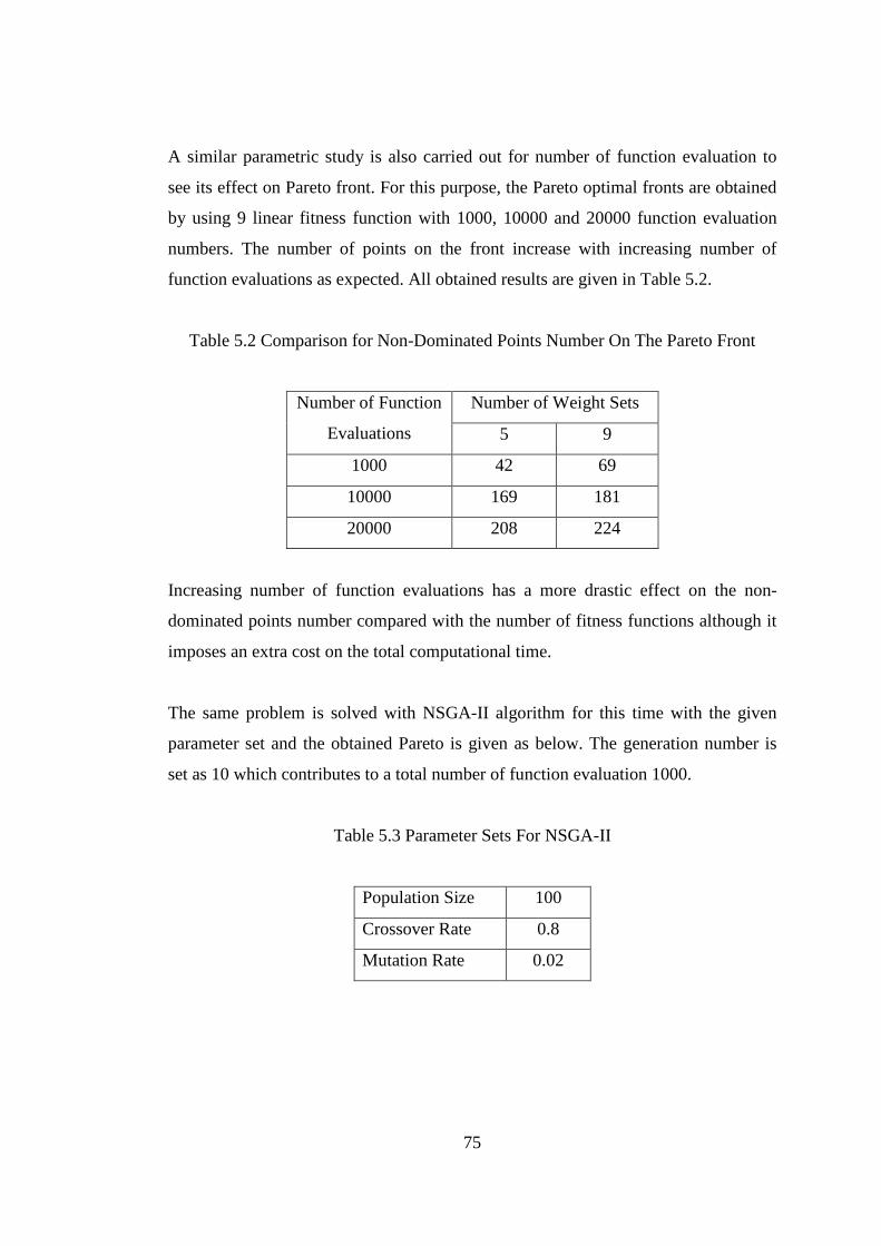
75
A similar parametric study is also carried out for number of function evaluation to
see its effect on Pareto front. For this purpose, the Pareto optimal fronts are obtained
by using 9 linear fitness function with 1000, 10000 and 20000 function evaluation
numbers. The number of points on the front increase with increasing number of
function evaluations as expected. All obtained results are given in Table 5.2.
Table 5.2 Comparison for Non-Dominated Points Number On The Pareto Front
Number of Function
Evaluations
Number of Weight Sets
5 9
1000 42 69
10000 169 181
20000 208 224
Increasing number of function evaluations has a more drastic effect on the non-
dominated points number compared with the number of fitness functions although it
imposes an extra cost on the total computational time.
The same problem is solved with NSGA-II algorithm for this time with the given
parameter set and the obtained Pareto is given as below. The generation number is
set as 10 which contributes to a total number of function evaluation 1000.
Table 5.3 Parameter Sets For NSGA-II
Population Size 100
Crossover Rate 0.8
Mutation Rate 0.02

76
Figure 5.5 Two Bar Truss Problem : NSGA-II Results After 1000 FEN
The results are in accordance for two distinct algorithms whereas the spread of the
solutions of MC-MOSA with 9 FFs is better than the NSGA-II algorithm. Moreover,
the number of points on the front is also more than the ones for the NSGA-II
algorithm.
0
20000
40000
60000
80000
100000
120000
0 0.01 0.02 0.03 0.04 0.05 0.06 0.07 0.08 0.09
ST
RE
SS
(k
Pa
)
VOLUME (m3)

77
Figure 5.6 Two Bar Truss Problem : MC-MOSA & NSGA-II Results Comparison
After 1000 FEN
The results of two algorithms are compared by the usage of some quality metrics for
1000 function evaluations. These metrics asserts the quality of the obtained Pareto
front. The metrics utilized for this purpose are Non-Dominated Points (NDP),
Hyperarea Difference (HD), Accuracy (A), Overall Spread (OS) and Cluster (CL).
The details of each are given in Appendix C. The resulting of the quality metrics for
each algorithm are tabulated in the table below.
Table 5.4 Comparison of Multi-Objective Optimization Algorithms for Two Bar
Truss Design Problem
MC-MOSA NSGA-II
NDP 69 53
HD 0.1541 0.1525
A 45.1 16.9
OS 0.5323 0.4531
0
10000
20000
30000
40000
50000
60000
70000
80000
90000
100000
0 0.01 0.02 0.03 0.04 0.05 0.06 0.07 0.08
ST
RE
SS
(k
Pa
)
VOLUME (m3)
MC-MOSA
NSGA-II

78
Table 5.4 Comparison of Multi-Objective Optimization Algorithms for Two Bar
Truss Design Problem (continued)
CL 1/50 1.3269 1.4722
CL 1/150 1.0500 1.1042
MC-MOSA algorithm is able to find more non-dominated points on the front than
NSGA-II algorithm for this problem. Even though smaller HD value for NSGA-II
algorithm claims for a better front, larger values for OS and A for MC-MOSA
algorithm indicates a Pareto front that is spread well to the extreme ends well. MC-
MOSA occupies more cell with both step sizes 50 and 150 which is also another
indication of a good spread front for MC-MOSA algorithm.
Test Problem-2 : Air-to-Ground Missile Conceptual Design Optimization 5.2
The aerodynamics, flight and the optimization modules constitute the overall
conceptual design tool. The verification of the tool is realized by applying it for a
new generation existing turbojet powered air-to-ground missile (i.e. Naval Strike
Missile (NSM)) that has a pair of wings and four tails and it is controlled by
deflecting tail control surfaces. The flight profile is assumed to be a glide-descent-
cruise-climb-dive sequence. The detailed technical specifications and external
geometry parameters, mission requirements and constraints for the benchmark
missile is obtained from the open sources available.
The weight of the missile is a bit more than 400 kg and it has a range of at least 185
km. “After being launched into the air by a solid rocket booster which is jettisoned
upon burning out, the missile is propelled to its target in high subsonic speed by a
turbojet sustainer engine leaving the 125 kg multi-purpose blast, fragmentation
warhead to do its work” [44]. Furthermore it is aimed to achieve approximately 0.9
Mach top speed.

79
Figure 5.7 Naval Strike Missile (NSM) [44]
The Microturbo TRI-40 turbojet engine supplies the thrust force for the NSM
missile. The maximum thrust value that the engine could generate is 2500-3500
Newtons. It is 0.68 meters long and 0.28 meters in diameter. The diameter of the
engine imposes a physical constraint on the diameter of the missile such that it
should be greater than the engine diameter [45].
Some other inputs required for the tool like cruise and search altitudes, descent and
climb angles, wing and tail airfoil types are not available in the internet. Thus, a set
of values for these parameters are chosen and listed in Table 5.5.
Table 5.5 Parameters selected for NSM
Search Altitude (m) 1750
Cruise Altitude (m) 300
Descent Angle (°) -15
Climb Angle (°) 15
Wing Airfoil Section NACA-1-6-65-410
Tail Airfoil Section HEX
The missile length is given as 3.96 meters. Unfortunately, there is no other geometric
dimension available. To specify other geometric variables, a sample picture of the
missile found from the open sources is transferred into a computer aided drawing
tool and its length is scaled with respect to the given real missile length. Such
estimated parameters are summarized in Table 5.6.

80
Table 5.6 NSM Estimated Geometry Parameters In Meters
Missile Length 3.96
Wingspan (tip-to-tip) 0.835
Wing Tip Chord 0.2
Wing Root Chord 0.6
Tail Span (tip-to-tip) 0.8
Tail Tip Chord 0.15
Tail Root Chord 0.38
5.2.1 Single Objective Optimization
The missile design optimization problem is solved for single objective, first. The
objectives are decided to be as maximum range and minimum launch mass as stated
earlier.
For maximum range objective, an upper bound constraint is imposed on the initial
launch mass such that the designed missile is desired to be weighed less than 450 kg.
The problem is solved with Hide-Seek Simulated Annealing, Genetic Algorithm and
the Hybrid Algorithm (Hide-Seek SA + GA). The maximum number of function
evaluation is selected to be as 1000 for each algorithm and the population size is set
to 100. The obtained results are given in Table 4.1 below and compared with the
parameters belonging to NSM.

81
Table 5.7 External Configuration Parameters for Range Objective Case
According to the obtained results, the hybrid algorithm is able to find the missile that
could reach the maximum range with minimum launch mass. The external
parameters are noticed to be in accordance with the existing benchmark missile.
Furthermore, SA has achieved to find a better design than GA for this case (mass
objective design problem) although it comes out be a heavier missile than the GA’s.
Afterwards, the launch mass was tried to be optimized for a given at least flight
range limit ( > 200 km) and the obtained results for each three single objective
optimization algorithm including the comparison with NSM are tabulated in Table
4.1.
Ogive Ogive Ogive -
Cross Cross Cross Cross
0.32 0.30 0.30 -
0.29 0.54 0.63 -
0.45 0.78 0.67 0.84
0.23 0.55 0.51 0.6
0.17 0.13 0.18 0.2
0.18 0.19 0.34 0.4
0.43 0.23 0.44 0.38
0.40 0.12 0.23 0.15
4.45 3.58 2.47 -
4.75 4.40 3.73 -
2.59 2.32 2.08 -
7.85 28.33 26.78 -
11.25 30.43 31.25 -
LENGTH 5.19 4.63 4.16 3.95
424.4 380.7 362.6 410
42.4 38.1 36.3 -
246.0 232.0 250.9 over 185
0.75 0.75 0.75 high subsonic
960.4 849.0 976.1 -
NSM PARAMETERSSA Optimization
ResultsGA Optimization
Results
SA-GA Optimization
Results
Tail Sweep (deg)
EXTERNAL CONFIGURATION
PARAMETERS
Nose Type
Panel Config
Body Diameter (m)
Nose Length (m)
Wing Span (m)
Wing Root Chord (m)
Win Tip Chord (m)
Tail Span (m)
Tail Root Chord (m)
Tail Tip Chord (m)
Wing Leading Edge Location From Nose
Tail Leading Edge Location From Nose
CG location from nose (m)
Wing Sweep (deg)
Missile (m)
MASSLaunch (kg)
Fuel (kg)
FLIGHT PERFORMANCE
Range (km)
Cruise Mach
Time of Flight (sec)
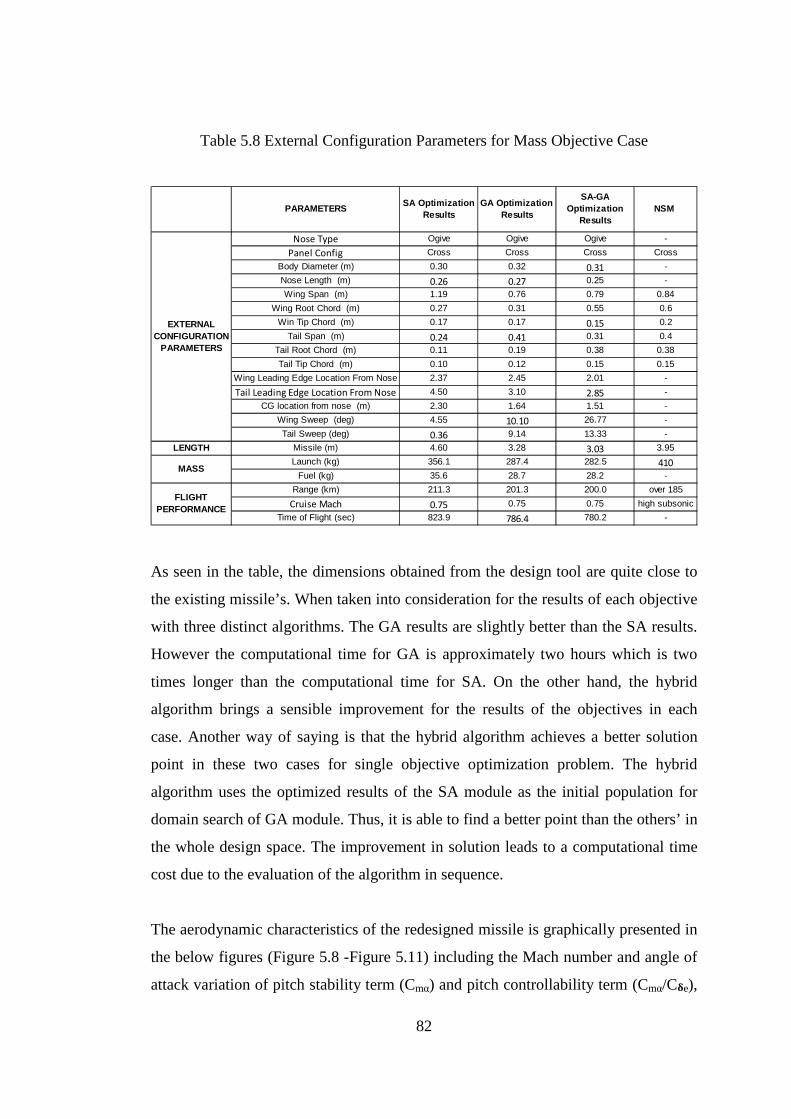
82
Table 5.8 External Configuration Parameters for Mass Objective Case
As seen in the table, the dimensions obtained from the design tool are quite close to
the existing missile’s. When taken into consideration for the results of each objective
with three distinct algorithms. The GA results are slightly better than the SA results.
However the computational time for GA is approximately two hours which is two
times longer than the computational time for SA. On the other hand, the hybrid
algorithm brings a sensible improvement for the results of the objectives in each
case. Another way of saying is that the hybrid algorithm achieves a better solution
point in these two cases for single objective optimization problem. The hybrid
algorithm uses the optimized results of the SA module as the initial population for
domain search of GA module. Thus, it is able to find a better point than the others’ in
the whole design space. The improvement in solution leads to a computational time
cost due to the evaluation of the algorithm in sequence.
The aerodynamic characteristics of the redesigned missile is graphically presented in
the below figures (Figure 5.8 -Figure 5.11) including the Mach number and angle of
attack variation of pitch stability term (Cmα) and pitch controllability term (Cmα/C�e),
Ogive Ogive Ogive -
Cross Cross Cross Cross
0.30 0.32 0.31 -
0.26 0.27 0.25 -
1.19 0.76 0.79 0.84
0.27 0.31 0.55 0.6
0.17 0.17 0.15 0.2
0.24 0.41 0.31 0.4
0.11 0.19 0.38 0.38
0.10 0.12 0.15 0.15
2.37 2.45 2.01 -
4.50 3.10 2.85 -
2.30 1.64 1.51 -
4.55 10.10 26.77 -
0.36 9.14 13.33 -
LENGTH 4.60 3.28 3.03 3.95
356.1 287.4 282.5 410
35.6 28.7 28.2 -
211.3 201.3 200.0 over 185
0.75 0.75 0.75 high subsonic
823.9 786.4 780.2 -
NSM PARAMETERSSA Optimization
ResultsGA Optimization
Results
SA-GA Optimization
Results
Tail Sweep (deg)
EXTERNAL CONFIGURATION
PARAMETERS
Nose Type
Panel Config
Body Diameter (m)
Nose Length (m)
Wing Span (m)
Wing Root Chord (m)
Win Tip Chord (m)
Tail Span (m)
Tail Root Chord (m)
Tail Tip Chord (m)
Wing Leading Edge Location From Nose
Tail Leading Edge Location From Nose
CG location from nose (m)
Wing Sweep (deg)
FLIGHT PERFORMANCE
Range (km)
Cruise Mach
Time of Flight (sec)
Missile (m)
MASSLaunch (kg)
Fuel (kg)
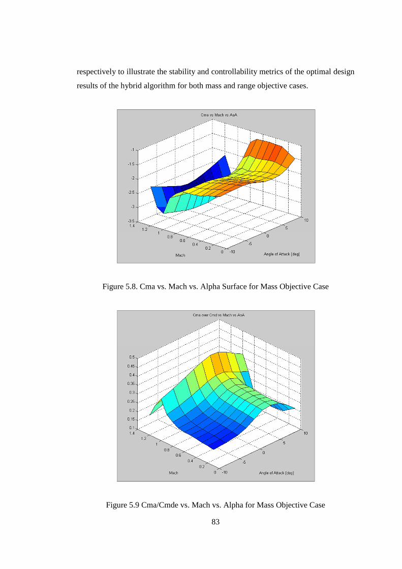
83
respectively to illustrate the stability and controllability metrics of the optimal design
results of the hybrid algorithm for both mass and range objective cases.
Figure 5.8. Cma vs. Mach vs. Alpha Surface for Mass Objective Case
Figure 5.9 Cma/Cmde vs. Mach vs. Alpha for Mass Objective Case

84
Figure 5.10 Cma vs. Mach vs. Alpha Surface for Range Objective Case
Figure 5.11 Cma/Cmde vs. Mach vs. Alpha Surface for Range Objective Case

85
All these obtained plots demonstrate that the missile geometries resulted from the
hybrid algorithm for each range and mass single objective cases are said to be
acceptable in terms of static stability (negative Cmα) and pitch controllability
(Cmα/C�e < 1) throughout the whole Mach number and angle of attack regime.
Additionally, the resultant dimensions for each designed geometry is visualized in
three dimensional (3D) view via importing the “for022.dat”. file, which is the output
of Missile DATCOM 2008 module, into a plotting program and presented in Figure
5.12.
Range Objective Mass Objective
Figure 5.12 Single Objective Missile Design Optimization Results
The geometry for maximum range objective is a long and slender body with a large
nose finess ratio which results in a body exposed to less drag during its flight. The
sketches on the left figures out a shorter missile. Moreover, the wing span is slightly
longer than the range objective case in order to satisfy the at least range constraint.

86
5.2.2 Multi-Objective Optimization
In this section, the two objective optimizations carried out using MC-MOSA and
NSGA-II multi-objective optimization algorithms are presented. In addition to that, a
hybrid algorithm, that sequentially uses MC-MOSA and NSGA-II combination, is
also tested through the design optimization problem. The Pareto optimal fronts are
obtained and compared.
The results of the MC-MOSA algorithm for 9 linear FFs and 1000 function
evaluation are given in Figure 5.13.
Figure 5.13 MC-MOSA Missile Design Optimization Results
As seen from the figure, although not too many points were generated on the front,
the non-dominated points are noticed to be sparse and scattered which is thought to
stem from the difficulty of the problem of optimization of two distinct conflicting
objectives.
250.0
300.0
350.0
400.0
450.0
500.0
550.0
600.0
650.0
700.0
160.0 180.0 200.0 220.0 240.0 260.0 280.0 300.0
MA
SS
[k
g]
RANGE [km]
RECORD POINTS
PARETO

87
The same two objective missile design optimization problem is also solved using
NSGA-II and hybrid algorithm and the results are presented in Figure 5.14 together
with the results of MC-MOSA with the same number of function evaluations. A
population size of 100 is used for 10 generations for NSGA-II algorithm. For the
hybrid case, the initial population is obtained as a result of 500 function evaluation of
MC-MOSA algorithm and then passed to the NSGA-II module for 10 generations
with 50 individuals in the population which leads to a 1000 function evaluations in
total.
Figure 5.14 Missile Design Multi Objective Optimization Results After 1000 FEN
For the current problem, the Pareto front of NSGA-II algorithm looks better when
compared with the front of MC-MOSA algorithm since it was able to find better
optimal points for present objectives. Approximately two times longer computational
time than the one for MC-MOSA algorithm is the payoff for better front, though. The
hybrid algorithm, carried out for an ultimate trial, indicated the capability of the
algorithm of finding more non-dominated points on the front that is closer to the
optimal than other algorithms.
200.0
250.0
300.0
350.0
400.0
450.0
500.0
550.0
600.0
650.0
700.0
160.0 180.0 200.0 220.0 240.0 260.0 280.0 300.0
MA
SS
[k
g]
RANGE [km]
MCMOSA 1000 FEN
NSGA II 1000 FEN
MCMOSA + NSGA II 1000 FEN

88
Since 1000 function evaluations is small for such a nonlinear problem, it was also
solved, this time allowing for 2000 function evaluations. The non-dominated
solutions from each algorithm are plotted in Figure 5.15.
Figure 5.15 Missile Design Multi Objective Optimization Results After 2000 FEN
The results of the algorithms for both 1000 and 2000 function evaluations are
compared by using the quality metrics defined in Appendix C and they are presented
in Table 5.9.
200.0
250.0
300.0
350.0
400.0
450.0
500.0
550.0
600.0
650.0
700.0
160.0 180.0 200.0 220.0 240.0 260.0 280.0 300.0
MA
SS
[k
g]
RANGE [km]
MCMOSA 2000 FEN
NSGA II 2000 FEN
MCMOSA + NSGA II 2000
FEN

89
Table 5.9 Comparison of Multi Objective Optimization Algorithms for Missile
Design Optimization Problem
MC-MOSA NSGA-II
MC-MOSA -
NSGA-II
1000
FEN
2000
FEN.
1000
FEN
2000
FEN.
1000
FEN
2000
FEN.
NDP 16 18 16 21 7 23
HD 0.2096 0.1541 0.1433 0.1 0.1310 0.0957
A 39.7 65.82 56.2 48.53 31.4 135.2
OS 0.1777 0.1605 0.1381 0.3924 0.1673 0.2426
CL 1/25 1.23 1.25 1.1429 1.2609 1.1500 1.2
CL 1/100 1.14 1.25 1.043 1.1154 1.0952 1.0714
It could be noticed that an increase in the number of function evaluations lead to an
increase in the number of non-dominated points on the front as well as a smaller HD
value which is an indication of a better Pareto front. The results also figure out that
NSGA-II algorithm has performed better than MC-MOSA algorithm for design
optimization problem for both 1000 and 2000 function evaluation number with
smaller HD values whereas the front has not covered the whole region better than
MC-MOSA algorithm due to a smaller OS value for 1000 function evaluation
number. As the number of function evaluations are increased, the spread over the
whole feasible region seemed to be better for NSGA-II algorithm. Also, NSGA-II
occupied more cells with both step sizes 25 and 100.
The results of the hybrid algorithm brings a noteworthy improvement in the Pareto
front accuracy with less HD and larger A value, especially for 2000 function
evaluation number which comes out to be the best front obtained in terms of
optimality. More non-domniated points closer to the actual front are also obtained
with the hybrid algorithm for 2000 function evaluations and it has also better values
for the remaining metrics. Therefore, the fact that the hybrid algorithm has a better

90
solution performance than other algorithms for multi-objective optimization, could
be drawn as a conclusion for this test problem.

91
CHAPTER 6
CONCLUSION
In this thesis work, several optimization techniques were utilized for the conceptual
design optimization problem of a generic air-to-ground missile. To initiate the design
cycle, a baseline missile external configuration was specified with two wings and
four tails powered with a turbojet engine. The external geometry parameters were
aimed to be optimized to satisfy the specified objectives and the feasible bounds
desired to be stayed in are all left to the designer to be determined at the beginning of
the optimization process. In addition to these, the geometric constraints for aircraft
launch compability are also imposed.
To decide on the optimal missile geometry that meets best with the user defined
requirements, a simulation tool was developed with two degrees of freedom trim
flight mechanics model. Its usage brought the advantage of the fast evaluation of the
flight performance of the candidate missile. At each step of the iteration, the
candidate missile was checked whether it satisfies the geometrical constraints as well
as the upper and lower bounds for each external configuration parameter. The loop
has been run interactively with Missile DATCOM aerodynamic prediction tool to
generate the aerodynamic database for the external geometry.
Since the conceptual design stage was the starting point for a whole missile design
process, it was aimed to carry out two main objectives: maximum flight range with
minimum launch mass. Hence, both single objective and multi-objective
optimization approaches were conducted with different algorithm alternatives that
gave way to carry out a comparative study between these solutions and algorithm
alternatives.

92
Hide-Seek Simulated Annealing, a Genetic Algorithm and a hybrid algorithm, a
combination of these two approaches, were utilized for single objective optimization
problem. The optimization tool was practiced for an existing cruise missile in order
to check whether the validation of the tool was satisfactory or not. The conceptual
design optimization tool was executed for two cases, both maximum flight range and
minimum launch mass objectives. The results showed that the results of the hybrid
algorithm was considerably accurate in terms of solution optimality for both
objective channel accordingly.
The main deficiency for single objective optimization case was that it gave only a
single solution in the whole design space that do not allow the user to make a trade
off between conflicting objectives during the design process. Therefore, a multi-
objective design optimization was also enforced. The range maximization problem
was converted into a minimization problem to prevent a sign confusion and
normalized with respect to the reference values together with the mass channel.
The multi-objective optimization missile design problem was solved with Multiple
Cooling Multi Objective Simulated Annealing (MC-MOSA) and Non-Dominated
Sorting Genetic (NSGA-II) Algorithms. Before proceeding, these algorithms were
applied for a well known multi-objective optimization problem, truss bar design to
test their solution accuracy in terms of quality metrics. The effects of algorithm
parameters on solution accuracy were also investigated.
First, the multi-objective optimization problem was solved with MC-MOSA
algorithm using linear FFs and NSGA-II algorithms. It was seen that the Pareto
obtained with NSGA-II algorithm was closer to the optimal front although it
consisted of less non-dominated points on the front. As a final trial, as in the case for
single objective optimization case, a hybrid algorithm was also used. The obtained
Pareto fronts for each three attempt were compared with each other using quality
metrics. Again, the results showed that the hybrid algorithm was able to find more
points closer to the optimal Pareto when same number of function evaluation is
permitted.

93
The obtained results prove that the conceptual design tool is capable of finding an
optimal external missile configuration satisfying the user defined requirements and
constraints in short durations even with single or multi objectives. This plays a vital
role in the missile design processes since it reduces the effort and time to find out the
optimum baseline geometry throughout a huge design domain.
The capabilities of the current tool could be enhanced. Several recommendations for
future improvements of the tool could be listed as below.
� The design objectives could be increased. Minimizing the radar cross section
(RCS), maximizing the hit accuracy and warhead effectiveness could also be
taken into account as design objectives.
� Better aerodynamic prediction tools other than Missile DATCOM could
probably be used in the future. Various cross sectional alternatives for
missile bodies could be taken into account by this way.
� The specifications for turbojet engine could be automized. The turbojet
engine that provides the necessary requirements would be specified that suits
geometrically with the designed missile.
� The scope of the conceptual design optimization of an air to ground missile
could be extended to cover other types of missiles like air-to-air and surface-
to-air missiles.

94
REFERENCES
[1] Fleeman, E. L. “Tactical Missile Design”, AIAA Education Series, USA. 2001
[2] Kirkpatrick, S., “Optimization by Simulated Annealing – Quantitative
Studies”, J. Stat. Phys. 34, 975-986, 1984.
[3] Bélisle C. J. P., Romeijn H. E., Smith R.L., “Hide-and-Seek: A Simulated
Annealing Algorithm for Global Optimization”, Department of Industrial and
Operations Engineering, Technical Report 90-25, University of Michigan,
Ann Arbor, 1990
[4] Lu, Ping and Khan, Asif, “Nonsmooth Trajectory Optimization: An Approach
Using Continuous Simulated Annealing”, Journal of Guidance, Control and
Dynamics, Vol.17, No.4, July-August 1994
[5] Utalay S., “Trajectory and Multidisciplinary Design Optimization of Missiles
Using Simulated Annealing”, M.S. Thesis, Aeronautical Engineering
Department, METU, Ankara, January 2000
[6] Bingöl, M., “Trajectory and Multidisciplinary Design Optimization of
Missiles Using Simulated Annealing”, M.S. Thesis, Aeronautical Engineering
Department, METU, Ankara, January 2000
[7] Karslı G., Tekinalp O., “Simulated Annealing For The Generation of Pareto
Fronts With Aerospace Applications”, M.S. Thesis, Aeronautical Engineering
Department, METU, Ankara, January 2004

95
[8] Öztürk M. Y., “Multi-objetive Design Optimization of Rockets and Missiles”,
M.S. Thesis, Aeronautical Engineering Department, METU, Ankara, March
2009
[9] Aytar Ortaç. S., “Optimal External Configuration Design of Missiles”, M.S.
Thesis, Mechanical Engineering Department, METU, Ankara, January 2002
[10] Tanıl. Ç., “Optimal External Configuration Design of Missiles”, M.S. Thesis,
Mechanical Engineering Department, METU, Ankara, July 2009
[11] Zeeshan. Q., Yunfeng D., Rafique A. F., Nisar K., Kamran A., “Meta
Heuristic Approach For The Conceptual Design And Optimization of
Multistage Interceptor”, 18th World IMACS/MODSIM Congress, Cairns,
Australia 13-17 July 2009
[12] Zipfel, P. H., “Modelling and Simulation of Aerospace Vehicle Dynamics”,
AIAA Education Series, USA. 2000
[13] Etkin B., Reid L. D., “Dynamics of Flight Stability and Control”, John Wiley
& Sons, Inc, 3rd Edition, 1996
[14] Auman L., Doyle J., Rosema C., Underwood M., “Missile DATCOM User’s
Manual 2008 Revision”, US Army Aviation & Missile Research,
Development and Engineering Centre, August 2008.
[15] Anderson Jr., J. D., “Aircraft Performance And Design”, McGraw Hill
International Editions, New York, USA ,1999.
[16] Carus.S. W., “Cruise Missile Proliferation In The 1990s”, The Washington
Papers, Washington D.C., USA, 1992

96
[17] MATLAB R2008b Aerospace Blockset, “WGS84-Gravity-Model”
http://www.mathworks.com/help/toolbox/aeroblks/wgs84gravitymodel.html,
(Last accessed date: October 10, 2010)
[18] Gary A., Crowell Sr., “The Descriptive Geometry of Nose Cones”,
http://www.scribd.com/doc/60921375/The-Descriptive-Geometry-of-Nose-
Cone
(Last accessed date: October 29, 2010)
[19] Chin SS., “Missile Configuration Design”, McGraw-Hill Book Co., Inc., New
York, 1961
[20] Raymer.D. P., “Aircraft Design :A Conceptual Approach”, 3rd Edition,
AIAA Education Series, USA, 1999
[21] Nowell Jr J. B., “Missile Total and Subsection Weight and Size Estimation
Equations”, M.S. Thesis, Naval Postgraduate School, June 1992.
[22] Wikipedia The Free Encyclopaedia, “Finess Ratio”
http://en.wikipedia.org/wiki/Fineness_ratio,
(Last accessed date: October 01, 2010)
[23] Blum C., Roli A., “Metaheuristics In Combinatorial Optimization : Overview
and Conceptual Comparison”, Journal ACM Computing Surveys, Volume 35
Issue 3, September 2003.
[24] Kirkpatrick S., Gelatt G. C., Vecchi M. P., “Optimization By Simulated
Annealing”, Science, Vol.220, No.4598, May 1983
[25] Nielsen J. N., “Missile Aerodynamics”, Library of Flight Series, AIAA
Education Series, USA, 1988.

97
[26] Mathematical Optimization, “Simulated Annealing”,
http://www.phy.ornl.gov/csep/CSEP/MO/NODE28.html,
(Last accessed date: October 12, 2010)
[27] “Coello, C. A.; “A Comprehensive Survey of Evolutionary-Based
Multiobjective Optimization Techniques”, Journal ACM Computing Surveys
(CSUR), Volume 32 Issue 2, New York, NY, USA, June 2000
[28] Lu, Ping and Khan, Asif, “Nonsmooth Trajectory Optimization: An Approach
Using Continuous Simulated Annealing”, Journal of Guidance, Control and
Dynamics, Vol.17, No.4, July-August 1994
[29] Holland J. H., “Outline of a Logical Theory of Adaptive Systems”, Journal of
ACM, Vol.3, 1962
[30] Venkataraman P., “Applied Optimization with MATLAB Programming”, John
Wiley & Sons, New York, USA ,2002
[31] Goldberg D., “Genetic Algorithms and Engineering Optimization”, Wiley
Series in Engineering Design and Automation, New York, 2000
[32] Introduction to Genetic Algorithms, “Routte Wheel Selection”
http://www.obitko.com/tutorials/geneticalgorithms/selection.php,
(Last accessed date: November 23, 2010)
[33] MATLAB R2008b Global Optimization Toolbox, “Scattered Crossover”
http://www.mathworks.com/help/toolbox/gads/f6174dfi10.html,
(Last accessed date: November 30, 2010)
[34] Lynch, M., "Evolution of the Mutation Rate, Trends in Genetic “,vol. 26, no.
436, pp. 345–352, 2010.

98
[35] “Empirical comparison of stochastic algorithms”
http://www.uwasa.fi/cs/publications/2NWGA/2NWGA.html,
(Last accessed date: December 12, 2010)
[36] Theodore W. M., James T. C., “ Genetic Algorithms vs. Simulated Annealing:
A Comparison of Approaches for Solving the Circuit Partitioning Problem.”
University of Pittsburgh, Dept. of Electrical Engineering, May 1996
[37] Jason W. M., George D. S., “A Comparison of Heuristics for
Telecommunications Traffic Routing” John Wiley & Sons, 1996
[38] Poulos P. N., Rigatos G. G., Tzafestas S. G., Koukos A. K., “A Pareto-
optimal genetic algorithm for warehouse multi-objective optimization,
Engineering Applications of Artificial Intelligence”, 14, pp. 737-749, 2001
[39] Deb K., Agrawal S., Pratap a., Meyarivan T., “A fast and elitist multi-
objective genetic algorithm: NSGA-II”, Technical Report 200001, Indian
Institute of Technology, Kanpur: Kanpur Genetic Algorithms Laboratory
(KanGAL), India, 2000
[40] Deb K., Multi-objective Optimization Using Evolutionary Algorithms, Wiley,
New York, USA, 2001
[41] Tekinalp, O., Karsli, G., “A New Multi-objective Simulated Annealing
Algorithm”, Journal of Global Optimization, Vol. 39, No. 1, 49-77, Sep.
2007.
[42] Özdemir S., “Multi-Objective Conceptual Design Optimization of an
Agricultural Aerial Robot (AAR)”, M.S. Thesis, Aerospace Engineering
Department, METU, Ankara, September 2005

99
[43] Çavuş N., “Multidisciplinary and Multi-objective Design Optimization of An
Unmanned Combat Aerial Vehicle (UCAV)”, M.S. Thesis, Aerospace
Engineering Department, METU, Ankara, February 2009
[44] Wikipedia The Free Encyclopaedia, “Naval Strike Missile”
http://en.wikipedia.org/wiki/Naval_Strike_Missile,
(Last accessed date: May 23,2011)
[45] Microturbo TRI 40/TRI 60,.”The Market for Missile/Drone/UAV Gas
Turbine Engines”, Forecast International, 2008.
[46] Wu, J., Azarm, S., “Metrics For Quality Assessment Of A Multi-objective
Design Optimization Solution” Set. ASME J. Mech. Des. 123, 18–25, 2001

100
APPENDIX A
USER INTERFACE FOR CONCEPTUAL DESIGN OPTIMIZATION TOOL
Fig
ure
A.1
Use
r In
terf
ace
For
Con
cept
ual D
esig
n O
ptim
izat
ion
Too
l

101
APPENDIX B
MISSILE DATCOM INPUT & OUTPUT FILES
B.1. Missile Datcom Input File
The necessary inputs for the execution of the Missile DATCOM program is written
into the file for005.dat as shown below.
CASEID CASE1
DIM M
DERIV DEG
$REFQ
XCG=2.63,
BLAYER=NATURAL,
$END
$AXIBOD
TNOSE=OGIVE,
POWER=1.0,
LNOSE=0.68,
BNOSE=0.01,
DNOSE=0.34,
LCENTR=4.57,
DCENTR=0.34,
$END
$FINSET1
SECTYP=NACA,
SSPAN=0.0,0.72,
CHORD=0.83,0.18,
XLE=2.96,
SWEEP=0.00,
STA=1.0,
NPANEL=2.0,
PHIF=90.0,270.0,
$END
NACA-1-6-65-410

102
$FINSET2
SECTYP=HEX,
SSPAN=0.0,0.11,
CHORD=0.18,0.12,
XLE=5.08,
SWEEP=0.00,
STA=1.0,
NPANEL=4.0,
PHIF=45.0,135.0,225.0,315.0,
$END
$FLTCON
NMACH=10.0,
NALPHA=10.0,
MACH=0.1,0.3,0.5,0.6,0.7,0.8,0.9,1.0,1.1,1.2,
ALT=100.0,100.0,100.0,100.0,100.0,100.0,100.0,100.0,100.0,100.0,
ALPHA=-10.0,-7.0,-4.0,-2.0,0.0,2.0,4.0,6.0,8.0,10.0,
$END
$FLTCON
BETA=0.0,
$END
$DEFLCT
DELTA1=0.0,0.0,0.0,0.0,
DELTA2=0.0,0.0,0.0,0.0,
$END
DAMP
SAVE
NEXT CASE
$DEFLCT
DELTA1=0.0,0.0,0.0,0.0,
DELTA2=-5.0,-5.0,5.0,5.0,
$END
DAMP
SAVE
NEXT CASE

103
B.2. Missile Datcom Output File
As a consequence of the execution of the MD707.exe file for the determined external
configuration and atmospheric flight conditions, the aerodynamic database is written
to the for006.dat output file. A small part of this is shown below as example.
Figure B.1 Missile Datcom Output File

104
APPENDIX C
QUALITY METRICS
The quality assessment of the frontier obtained as a result of multi-objective
optimization is conducted using four metrics proposed in [41] and [46] which are
namely as hyper-area difference (HD), overall Pareto spread (OS), accuracy of the
observed Pareto frontier (AC) and the cluster (CL).
The area below the Pareto frontier is called as the hyperarea difference. It is shown in
Figure C.1.
Figure C.1 Hyperarea Difference [46]
Points A and B define the bounding box around the Pareto front and HD is normally
calculated using normalized objectives. Generally speaking, it is clear that the
smaller the HD metric means that the observed Pareto solution set is the better [46].

105
Overall Pareto spread (OS) is the area of the maximum rectangle constructed using
the two extremes of the Pareto front (p1 and p2) as shown in Figure C.2. Again a
solution set with the largest OS value is generally an indication that a particular front
has spread to the extreme ends of the Pareto front, and consequently, it is
comparatively better than a front with a smaller value.
Figure C.2 Overall Spread [46]
Accuracy (A) is an indicator of the smoothness of the front. Areas of the small
rectangles constructed from neighbouring solutions are summed up (Figure C.3) to
obtain a total area and the inverse of this total area gives the value for this metric. If
the solution set contains all the actual Pareto solutions (i.e., a continuous Pareto
frontier), the total area would be zero, causing the A metric to be infinite. Thus, a
solution set with a large A value is better than the one with a smaller A value. It is
desirable to have the solutions spread uniformly along the front.

106
Figure C.3 Accuracy [46]
Another quality metric is defined as the CLµ metric (clustering) that occurs when too
many solutions are found at certain parts of the front, while other parts are empty.
For this purpose normalized objectives are divided into square grids of size µ
throughout the whole domain. Then, those rectangles occupied with a non-dominated
solution are counted. The total number of non-dominated solutions in the set is
divided to the number of occupied rectangles. Ideally, to have a good spread, each
rectangle shall be occupied by a single solution giving a CLµ metric equal to one.
For example, in Figure C.4, there are four solutions in the front, while only three
grids are occupied (i.e., CLµ = 1.25). Similarly, of the two solution sets having
almost equal number of solutions, the one with a smaller CLµ metric shall be
preferred.

107
Figure C.4 Cluster [46]