Embed Size (px)
Citation preview

1
External Debt and Economic Growth in Jordan: The Threshold Effect
Aktham Maghyereh Ghassan Omet
& Fadwa Kalaji
Faculty of Economics & Administrative Sciences The Hashemite University
Jordan
Abstract
The Jordanian economy has a serious external debt problem. Based on several indicators, it can be argued that foreign debt has reached an excessive level and has become an impediment to economic growth. This paper examines the impact of external debt on the performance of the Jordanian economy and determines its optimum level using new econometric techniques that provide appropriate procedures for estimation and inference. The findings of the study indicate that the optimal level of external indebtedness is about 53 percent of GDP. In other words, when the external debt exceeds this level, its impact on the performance of the Jordanian economy becomes negative. Correspondence to: Ghassan Omet Dean Faculty of Economics & Administrative Sciences The Hashemite University PO Box, 150459 Zarka Jordan Tel: 05 3826600; Fax: 05 3826613 E-Mail: [email protected]

2
I. Introduction:
Jordan occupies an area of about 89,000 square kilometers. With an annual growth
rate of about 3 percent, its 4.5 million population is considered to be one of the fastest
growing in the world. Furthermore, with an urbanization rate of about 70%, life
expectancy of about 70 years and literacy rate of around 85%, Jordan's demographic
profile resembles that found in advanced economies. However, with a per capita GDP
of around $1550, Jordan is considered one of the poor countries in the world.
It is well - known that Jordan's natural resource base is relatively limited. Other than
phosphate and potash, the country does not have any natural resources. Indeed, this is
why, traditionally, the economy has relied on external debt, remittances and foreign
aid in managing its economic affairs.
Analyzing the economic performance of Jordan is very difficult. The country has
passed through many disturbances and these make the detection of any underlying
economic trends an extremely difficult task. However, since the end of the 1991 Gulf
crisis and its economic impact, the Jordanian economy has been passing through
relative stability albeit at a slow rate of economic growth.
The Jordanian economy enjoyed some high growth rates during the period 1973 -
1982. During this period, economic growth stood at an annual average of 11.6% in
real terms. This period was characterized by high exports to regional markets, rising
worker's remittances and Arab and foreign assistance and loans. Following this
period, the slowdown in regional economies and the resultant fall in remittances had
3
severe repercussions on the economy. Real economic growth during the period 1983 -
1988 decreased to an annual average of about 2.2%. By the end of 1988, the deficit in
the general budget was equal to about 25% of GDP and the total external debt was
more than 190% of GDP. As a result, the Government devalued the Jordanian Dinar
(JD), liberalized the foreign exchange market and embarked on a decade-long
austerity and restructuring program supervised by both the International Monetary
Fund (IMF) and the World Bank (WB).
The Gulf crisis (1990-1991) and the "temporary" loss of Iraq as the principle market
for exports exacerbated Jordan's economic problems. However, and not withstanding
these problems, the government has persevered with its economic policies. During the
early 1990's, real GDP grew at an average annual rate of about 7% and this was
largely due to those who returned from the Gulf (with capital) during and after the
crisis. It is well-known that annual remittances accounted for about 25 percent of
GDP during the 1990s. Since 1996, however, the pace of economic growth has
slowed down and with a real GDP growth rate of about 1.2% in 1997, 2.2% in 1998
and an estimated 1-3% in 1999 and 2000, the economy's performance remains
sluggish.
Relative to the current economic stability and somewhat sluggish performance of the
economy, there remain a number of important problems and these are unemployment,
poverty, and a chronic balance of trade deficit. It is believed that the unemployment
rate is currently around 15% of the labour force and poverty is estimated to be around
25% of the population. Moreover, it is well-known that the Jordanian economy has
been suffering from a chronic trade deficit problem. In 1999, 2000 and 2001, for

4
example, the trade deficit was equal to $1.89 billion, $2.71 billion, and $2.55 billion
respectively. These values represent an annual mean of about 25% of GDP.
Table 1 reports the size of Jordan’s stock of external debt and debt service ratios
during the last few years (1997-2001).
Table 1 Jordan’s External Debt Stock and Debt Service
Year 1996 1997 1998 1999 2000 2001
Outstanding External Debt ($ Billion)
6.50 7.14 7.62 7.87 7.21 7.10
External Debt as Percent of GDP 99.2 89.2 89.3 89.9 80.0 76 Debt Service Ratio (Cash Basis %) 15.8 14.8 14.4 14.1 15.0 - Debt Service Ratio (Commitment Basis %)
25.9 24.1 21.9 22.0 20.7 -
Source: Various Central Bank of Jordan Monthly Reports.
The difference between the cash and commitment basis of the debt service ratio
implies that the Kingdom could not meet its annual debt payments. Moreover, the
decrease in the debt size during the period 2000/2001 was largely due to the debt
write-offs provided by the USA. Finally, it is worth noting that a high proportion of
Jordan’s debt originates from official sources. For example, about 33% and 30% of
the external debt was from multilateral institutions (like the IMF and World Bank)
and bilateral loans (largely from Japan and Germany) respectively. Similarly, export
credit guarantees from countries like Germany, France, Japan, UK and the USA,
accounted for about 26% of the outstanding external debt in 2001.

5
Based on this brief account of Jordan’s external debt, one cannot underestimate its
importance. The large transfers that could be allocated to investment and
consumption are being channeled abroad. Indeed, this may act as a disincentive not
only to invest but also to adopt adjustment programs to increase economic growth.
Notwithstanding Jordan’s economic problems, successive governments have
persevered with some consistent policies and, currently, the country is committed to
the followings principles and policies:
- Private sector development
- Export promotion
- Privatization
- Local, Arab and foreign investment promotion
- Utilization of information technology for development
In addition, Jordan has made the decision to liberalize its trade regime and integrate
with the world economy by joining the World Trade Organization (WTO) and signing
the Association Agreement with the European Union. In other words, Jordan has
decided to become an integral part of “economic globalization”.
Given Jordan’s economic circumstances,, it can be stated that the challenge is to
succeed in creating a dynamic economy which is able to compete regionally and
internationally, increase real GDP growth by more than the increase in population,
reduce dependence on external transfers, reduce poverty and unemployment and

6
finally, to reduce the external debt overhang. This is why current economic policies
are committed to the principle of economic liberalization.
Jordan’s privatization process was launched in 1997 as part of the economic reform
plan. The privatization law (No. 25 / 2000) was approved by the Lower House of
Parliament in May 2000. This law established the Privatization Council to oversee the
process through the Executive Privatization Commission and to decide on the use of
privatization proceeds through the Privatization Proceeds Fund.
Similar to most privatization programs, the overall objectives of privatization in
Jordan include increasing efficiency of state-owned enterprises, expansion of
investment by private sector financing, raising revenues to the treasury and signaling
the government’s commitment to economic reform. The privatization process started
in 1998 with the sale of a 33% stake in the Jordan Cement Manufacturing Company
to the French-based Lafarge Group. Table 2 reports a summary of the completed
privatization deals.
Clearly, the largest privatization achievements were implemented by means of a sale
of shares to a “strategic” partner. In other words, the hitherto existing experience
shows that the government favours a foreign strategic partner over the sale of shares
through the Jordanian (or other) capital market (Amman Securities Market).
According to official reports, this method was chosen due to several reasons. First, a
strategic partner is more likely to invest in capital projects. Second, a strategic partner
would encourage improvements in efficiency and profitability.

7
Table 2
Summary of Completed Privatization Transactions
Company & Date Size and Type of Privatization Public Transportation Company (Sept. 1998)
10-year contract with three local companies ($0.5 million annual fee).
Jordan Cement Company (Dec. 1998)
33% of shares sold to strategic partner; LaFarge of France ($102 million)
Water Authority of Jordan (April 1999)
4-Year performance-based management contract; consortium led by the French company Suez Lyonnaise des Eaux ($2.2 million annual fee)
Royal Jordanian Duty Free Shops (August 2000)
Sold to the Spanish airport retail group; Aldeasa ($60.1 million)
Telecommunications Company (January 2000)
Sold 40% stake to a consortium led by FranceTelecom and Arab Bank ($508 million) and to Jordan Social Security Corporation ($114 million).
The literature about the relationship between external debt and growth or the effect of
debt on growth can be summarized by three strands of thought: The first sees external
debt as a capital inflow with a positive effect on domestic savings and investment and
thus on growth. This argument implies that foreign savings complement domestic
savings and investments (Eaton, 1993). The second strand considers external debt as a
substitute to domestic savings and investment and therefore tends to crowd them out
(Krugman, 1988; Alesina and Tabellini, 1989; and Tornell and Velasco, 1992). The
argument here runs as follows. If future debt is going to be greater than a country’s
ability to repay its loans, the expected debt service will be an increasing function of
its output level. In other words, the returns from investing in a country are seen as
being subjected to a high marginal tax by creditors and this might discourage
domestic and foreign investors. These models or theories are known as the debt
overhang theories. Finally, more recent studies have attempted to reconcile the above
conflicting views by developing models with non-linear effects of debt on growth.
For example, Cohen and Sachs (1986) and Cohen (1991, 1992) present endogenous

8
growth models where capital accumulation is the sole force driving growth.
Countries’ access to international financial markets is limited because of the risk of
debt repudiation. Growth is high in the early stages as the country borrows and
invests. Later on, growth falls to a lower level, and this new level would be higher
than it would have been had there been no international borrowing and lending
(financial autarky). The stage of repaying countries’ debts does not crowd out
investment because lenders are more patient and value growth more than the debtor
countries themselves. This result, however, depends on the ability of lenders to
implement optimal rescheduling policies. If they are not able to commit themselves to
this policy, a debt overhang scenario will occur and investment and growth in the
later stages will be even lower than in financial autarky.
Another relevant theoretical model is developed by Calvo (1998). This model links
the debt and growth problem to capital flight. In his model, Calvo shows that high
debt levels are associated with low growth since a higher distortionary tax burden on
capital is required to service debt, leading to a lower rate of return on capital, and
lower investment and growth. Low debt regimes have high growth rates for the
opposite reasons. Thus, the empirical implication of these models is a non-linear
effect (threshold effect) of debt on economic growth. In other words, these models
suggest that the effect of debt could become negative when external indebtedness
becomes excessive. It is necessary, therefore, when examining the relationship
between debt and growth, to take into account the existence (if any) of the threshold
effect. In other words, it is useful to determine at what level the effect of external
indebtedness on economic growth becomes negative.

9
While there have been several attempts to empirically assess the external-economic
growth link (see among others, Borensztein, 1990; Iyoha, 1996; Mbire and Atingi,
1997; Fosu, 1999; and Were, 2001), few studies consider the possibility of the
existence of non-linear growth effects of external debt. Elbadawi et al. (1997) and
Pattillo et al. (2001) are the only researchers that directly considered the non-linear
effects of debt on growth. They present fixed and random effects panel estimation of
a growth regression in which external debt enters both in a linear and quadratic form.
They report growth maximizing debt to GDP ratios equal to 97 percent and 70
percent respectively.
Given the fact that the Jordanian economy faces some serious challenges including its
“large” external debt, it is felt important and timely to investigate the following
question: At what level (if any) does the external debt level start to have a negative
impact on the performance of the Jordanian economy? In other words, what is the
“optimal” level of debt in the Jordanian economy?
Since we believe that this issue (threshold effect) is very much country-specific, the
results of the above-mentioned studies need to be interpreted carefully and may not
be easily extrapolated to general statements. In other words, there is a need for case-
by-case studies that take into consideration each country’s unique characteristics.
Furthermore, our paper differs from the above attempts in that we use new
econometric methods for the threshold estimation. These methods have recently been
developed by Hansen (1996, 1997; 1999 and 2000a,b) and Caner and Hansen (2000).

10
The rest of the paper is organized as follows. In Sections II and III, we discuss the
methodology and the statistical properties of the data respectively. The empirical
results are presented and discussed in Section IV. Finally, Section V summarizes and
concludes the papers.
II. Empirical Methodology
Following the endogenous growth models (known as the AK models) developed by
Romer (1986), Lucas (1988) and Pagano (1993), we use the following specification to
examine the relationship between external debt and economic growth after taking into
account the possibility of the existence of a threshold effect:
( )
;,....101
1][43210
Ttifif
d
XdGWAPINVy
t
tt
ttttttt
=≤>
=
+′+−++++=
∗
∗
∗∗
ππππ
εθππαπαααα π
where ty is the growth rate of real GDP, measured by the first difference in the
logarithm of the real GDP series, INV is gross capital formation as a proportion of
GDP (the effect of physical capital accumulation), GWAP is the growth rate of
working age population (the effect of human capital accumulation), π is the share of
external debt to GDP, ∗π is the threshold level of external debt, and ∗πd is a dummy
variable that takes the value of one to external debt level greater than ∗π percent and
zero otherwise. tX is a vector of control variables and these include terms of trade
(TRAD), inflation rate (INF), measured by the first difference in the logarithmic of
the CPI series, and government expenditure (current) as a share of GDP (GEX). tε is

11
the error term, which represents measurement errors in the independent variables, and
any other explanatory variables that have been omitted. This term is assumed to be
independently and identical normally distributed with zero mean and constant
variance, )),0( 2εσε iidNt ≈ . The subtraction of ∗π from π makes the relationship
between growth and external debt, described by equation (1), continuous at the
threshold level ∗π 1.
In the above model, the effect of external debt on GDP growth is given by 3α when
external debt is less than or equal to the optimal external debt level ( ∗π ), and by
43 αα + when external indebtness is higher than the optimal one.
Note that tX contains a number of variables among a large set found in the empirical
growth literature because very few of these variables pass the robustness tests in
Barro (1991), Mankiw et al. (1992) Levine and Renelt (1992), Barro and Sala-I-
Martin (1995) and Sala-I-Martin (1997). In this paper, we include the inflation rate
and the ratio government expenditure to GDP as indicators of macroeconomic
stability, and terms of trade to capture the degree of openness of the economy.
Staking the observation in vectors yields the following compact notion for equation
(1):
( )2,...,πππβπ =+= eXyt
1Continuity of the relationship given by equation (1) is desirable, otherwise small changes in the external debt level around the threshold level will yield different impacts on growth depending on whether external debt is increasing or decreasing.
12
where )( 43210 ′′= θαααααβπ is the vector of parameters and X is the
corresponding matrix of observations on the explanatory variables. The coefficient
vector β is indexed by π to show its dependence on the threshold level of external
debt, the sign of which is given by π andπ . Given that ( )π1s is the residual sum
squared with threshold level of external debt at π estimated using least-squares, the
optimal threshold level of external debt is chosen that minimize ( )π1s
( ){ } ( )3,...,,minarg 1 ππππ S=∗
It is important to determine whether the threshold effect is statistically significant.
The hypothesis of no threshold effect in equation (1) can be represented by the
following null hypothesis: )0:( 40 =αH . Under 0H the optimal external debt ( ∗π ) is
not identified, so classical tests have non-standard distributions. Hansen (1996, 1997,
1999, and 2000a,b) suggested a bootstrap method to simulate the asymptotic
distribution to test 0H using the likelihood ratio
( )4)(
)()( 2
10
πσπ
πSS
LR−
=
where 0S and ( )π1s are the residual sum of squares under 0: 40 =αH and 0: 41 ≠αH ,
respectively; and ( )πσ 2 is the residual variance under 1H . In other words, 0S and
( )π1s are the sum square errors from estimated equation (1), using the Ordinary Least
Square Method (OLS), with and without threshold effects, respectively. The
13
asymptotic distribution of LR is non-standard, and strictly dominates the
2kχ distribution. Hansen (1996, 1999, and 2000a,b) argues that because the
distribution of 1LR depends on the moments of the sample, the critical values cannot
be tabulated. He shows that a bootstrap procedure attains the first-order asymptotic
distribution, so the p-value constructed from the bootstrap is asymptotically valid2.
Prior to applying the estimation procedure mentioned above, it is important to
consider whether the variables under consideration are stationary. We test for
stationarity to ensure that the variables used in the regressions are not subject to
spurious correlation. The Augmented Dickey-Fuller (ADF) and the Phillips-Perron
(PP) units root tests are used to investigate the stationary status of each variable under
consideration.
III. Data Description
The annual (1970-2000) data source for all the variables under consideration is
compiled from various issues of the “Monthly Statistical Bulletin” published by the
Central Bank of Jordan. Table 3 provides summary statistics for the variables.
As can be seen, all variables, except for the growth of working age population, do not
significantly depart from the normal distribution (values of skewness and kurtosis are
0 and 3 respectively, if the observed distribution is normal). The Jarque-Bera test
statistics for normality are also low and insignificant (either at the 1% level or at the
5% level) for all variables, except for the growth of working age population. This
2 See Hansen (1996) for more details about how to bootstrap the distribution of LR .

14
suggests that the null hypothesis of these variables conforming to a normal
distribution cannot be rejected. The growth of working age population shows
significantly high values of kurtosis (8.88) indicating that for a given level of standard
deviation, observations of this variable cluster around a central point with a small
number of large outliers. The Jarque-Bera test statistic is highly significant suggesting
that growth of working age population departs significantly from the normal
distribution.
Table 3
Summary Statistics ty is the growth rate of real GDP measured by the first difference in the logarithm of
the real GDP series. INV is gross capital formation as a proportion of GDP, GWAP is growth of working age population, π is the share of external debt to GDP, TRAD is terms of trade, INF is inflation rates (INF) measured by the first difference in the logarithmic of the CPI series, and GEX is government expenditure (current) as a proportion of GDP. ADF is the Augmented Dickey-Fuller test. PP is the Phillips-Perron test. The null hypothesis tested that the relevant series contains a unit root against the alternative that it does not. *, **, and *** are significant at the 1%, 5%, and 10%, respectively
y GWAP INV π INF TRAD GEX
Mean 0.042 0.036 0.262 0.571 0.073 0.842 0.267 Median 0.033 0.031 0.263 0.279 0.064 0.843 0.265 Maximum 0.211 0.131 0.471 1.684 0.229 1.090 0.325 Minimum 0.167 -0.026 0.119 0.197 0.001 0.640 0.222 Std. Dev. 0.081 0.026 0.078 0.499 0.054 0.105 0.025 Skewness 0.007 1.806 0.421 0.215 0.973 0.206 0.508 Kurtosis 3.349 8.882 3.268 2.931 3.684 2.576 3.195 Jarque-Bera 0.148 57.573* 0.976 0.406** 5.138*** 0.437 1.339 ADF in level 2.304 -2.139 2.636 -1.315 1.677 2.295 1.686 PP in level 2.609 2.707** 2.268 -1.497 2.671 4.595* 2.264 ADF in 1th difference 4.160* 2.9983** 3.232** 2.960*** 3.028** 2.895*** 4.128* PP in 1th difference 6.786* 4.0181* 3.619** -5.228* 5.412* 8.652* 6.507*
As mentioned above, prior to applying the estimation procedure, it is important to
consider whether the variables of interest are stationary. For this purpose, we perform
a unit root test using both the ADF and PP tests. These tests are applied to the level

15
variables as well as to their first differences. The second half of Table 3 provides the
results of the unit root test of each variable of interest. The reported results indicate
the presence of a unit root (levels) in all variables. In other words, the null hypothesis
that each of the time series has a unit root cannot be rejected at the 5% level in both
tests. However, there is no evidence from either test that supports a unit root in the
first difference of all the variables. These results are broadly consistent with the
hypothesis that the variables under investigation are individually integrated of the
order one I(1). Therefore, it is necessary, before we perform the test procedure, to
transfer the variables of interest by taking their first difference operator to achieve
stationarity3. However, one may argue that differencing the variables leads to some
loss in their long-run properties. To test for the long-run relationship between
economic growth and its determinants, we use the Engle-Granger two-step co-
integration test. We generate the residuals series from the long-run equation of the
non-stationary variables, and then we test for the existence of a unit root in this series
using both the ADF and PP tests. If the null hypothesis that the residual series has a
unit root is rejected, we can conclude the there is a stable long-run relationship that
ties together with the evolution of real GDP growth and the evolution of its
determinants.
As a first step in exploring the bivariate relationship between growth and debt, Figure
1 plots the evolution of growth and debt over time. The figure shows that the debt
ratio has peaked in the late 1980s. Growth appears to be positively correlated with
debt when debt levels are relatively low and this relationship becomes negative at
3 Another advantage of running regressions using first differences of the data is to reduce any influence of multicollinearity, thus improving the robustness of the estimation results.

16
higher levels. These observations provide some pre-evidence that there is a non-linear
relationship between external debt and growth. Thus, it is possible, in principle, to
estimate the inflexion point, or threshold, at which time the sign of this relationship
changes.
-50
0
50
100
150
200
70 75 80 85 90 95 00
Growth Rate of Real GDP
External Debt/GDP
Figure 1. Growth and External Debt Over Time
Table 4 presents the correlation matrix among the variables. The first number is the
correlation coefficient and the second is the P-value (a value of less than 0.05
indicates that the correlation is significant at the 5% level). As can be seen, the ratio
of external debt to GDP is negatively and statistically correlated with growth.
However, finding a negative correlation between external debt and growth suggests,
but clearly does not prove that low levels of external debt imply higher growth. Part
of the correlation may be spurious, reflecting the effect of other factors (traditional
growth determinants) and the non-linearity of the debt-growth relationship posited by
theory. In the next section, we examine the non-linearity (threshold effects) in the
debt-growth relationship using the multivariate regression analysis described above.

17
Table 4 Estimated Correlation Matrix of Variables
y GWAP INV π INF TRAD GEX
y
1.00000 -0.33921 0.47559 -0.45209 -0.33693 0.10947 0.15355
GWAP
-0.33921 1.00000 0.20108 0.18711 0.01549 0.01982 -0.34433
INV
0.47559 -0.20108 1.00000 -0.03845 0.02572 0.10766 0.182610
π
-0.45209 0.18711 -0.0384 1.00000 0.11194 0.39764 -0.29370
INF
-0.33693 0.01549 0.02572 0.11194 1.00000 0.12928 0.58643
TRAD
-0.10946 0.01980 0.10766 0.39764 0.12928 1.00000 0.03849
GEX
0.15355 -0.34433 0.18261 -0.29370 0.58644 0.03849 1.0000
Note: For the definition of the variables see Table 3.
A. Test for the Unknown Threshold Effect
The first step in the analysis is to test for the existence of a threshold effect in the
relationship between real GDP growth and external debt using the likelihood
ratio, LR , discussed above. This is established by estimating equation (1) in the first
difference and computing the residual sum of squares (RSS) for the threshold levels
of external debt levels ranging from π to π . The optimal threshold level (external
debt level) is the one that minimizes the sequences of RSSs. Table 5 summarizes the
test results.
The first column provides the range over which the search for the optimal external
debt level is conducted. The range lies between π =30 and π =100 with increments of
1 percent. This procedure yields 70 regressions of equation (1). As can be seen from
the second column of Table 5, the smallest residual sum squared is found by setting
the optimal external debt level at the 53 percent level. The third column in Table (4)
18
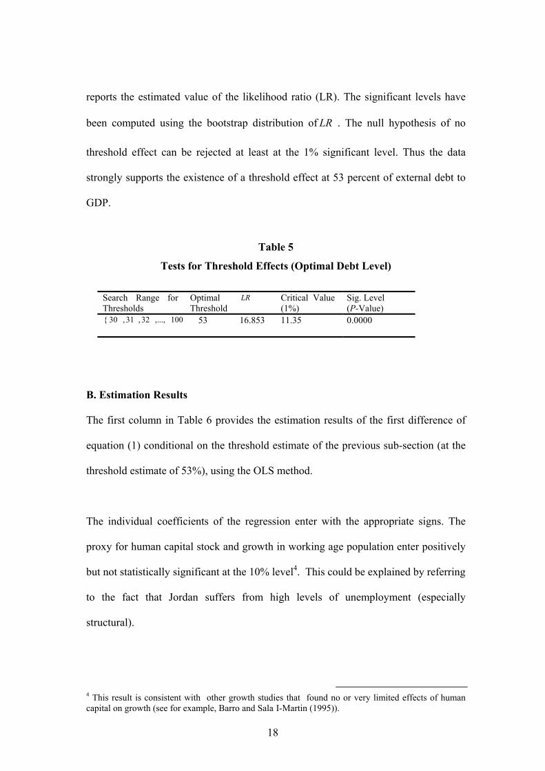
reports the estimated value of the likelihood ratio (LR). The significant levels have
been computed using the bootstrap distribution of LR . The null hypothesis of no
threshold effect can be rejected at least at the 1% significant level. Thus the data
strongly supports the existence of a threshold effect at 53 percent of external debt to
GDP.
Table 5
Tests for Threshold Effects (Optimal Debt Level)
Search Range for Thresholds
Optimal Threshold
LR Critical Value (1%)
Sig. Level (P-Value)
100,...,32,31,30{
53 16.853 11.35 0.0000
B. Estimation Results
The first column in Table 6 provides the estimation results of the first difference of
equation (1) conditional on the threshold estimate of the previous sub-section (at the
threshold estimate of 53%), using the OLS method.
The individual coefficients of the regression enter with the appropriate signs. The
proxy for human capital stock and growth in working age population enter positively
but not statistically significant at the 10% level4. This could be explained by referring
to the fact that Jordan suffers from high levels of unemployment (especially
structural).
4 This result is consistent with other growth studies that found no or very limited effects of human capital on growth (see for example, Barro and Sala I-Martin (1995)).

19
Table 6 Estimation Results
;,....101
][43210
Ttifif
d
XdGWAPINVy
t
tt
ttttttt
=≤>
=
∆+∆′+−∆+∆+∆+∆+=∆
∗
∗
∗∗
ππππ
εθππαπαααα π
D.W. is the Durbin-Watson test for residual serial correlation. The F-test tests the null hypothesis that all coefficients except for the intercept are zero. The reported misspecification tests are conducted to test a number of null hypotheses on the residuals. These tests are )1(2scχ , )1(2 ffχ , )2(2 nχ , )1(2hχ , ARCH which are defined respectively as follows: )1(2scχ = Serial correlation; Lagrange multiplier test of residuals serial correlation. )1(2 ffχ is the functional form; Ramsey’s REST test using square fitted values. )2(2 nχ =Normality, based on a test of skewness and kurtosis of residual. )1(2hχ is heteroscedasticity, based on the regression of squared residual on squared fitted values. ARCH is the autoregressive conditional heteroscedasticity test. Finally, ADF and PP are residual-based Augmented Dickey-Fuller test and the Phillips-Perron test of cointegration. Heteroscedasticity-consistent t-statistics in parentheses. *, **, and *** are significant at the 1%, 5%, and 10%, respectively For the definition of the variables see Table 3.
OLS 2SLS
Constant -0.6827*** (-1.883)
-0.7869*** (-1.7840
INV 0.3699** (2.0464)
0.2397** (2.2491)
GWAP 0.0628 (1.075)
0.0453 (0.983)
π 0.1555** (2.0475)
0.1288** (2.18400
D*(π - ∗π ) -0.6537** (-2.429)
-0.6926** (-2.362)
INF -1.1058* (-3.487)
-0.7256* (-3.827)
TRAD 0.3137** (2.117)
0.4963** (2.254)
GEX -0.4216 (-0.718)
-0.2331 (-0.4212)
2R 0.7135 0.832 F-statistic 6.0509* 7.516* D.W 2.0405 1.9998
)1(2scχ 0.4867 2.8651
)1(2 ffχ 0.0272 -
)2(2 nχ 4.2855 3.0905
)1(2hχ 1.0653 2.6849 ARCH(6) 0.0969 0.1326 ADF -3.6957** -3.4681** PP -5.0159* 6.4130*

20
The importance of investment (proxied by gross capital formation adjusted by GDP)
is emphasized by the strongly positive and statistically significant relationship that it
exhibits with economic growth5. A one-percentage point increase in investment to
GDP is associated with a 0.37 percentage point increase in real GDP growth rate.
This result is consistent with the theoretical view and empirical findings. Economic
theory holds that higher rates of savings and investments are important determinants
of the long-run growth rate. The suggestion behind Solow’s (1956) framework is that
higher investments and savings rates lead to more accumulated capital per worker and
this results in an increase in economic growth, but at decreasing rate. Under
endogenous growth theories that emphasize the broader concepts of capital (Rebelo,
1991), economic growth and investment tend to move together.
Government expenditure (current) as a percentage of GDP enters negatively but not
statistically significant at the 10% level. The explanation of this result can be found in
the supply side theories since the Jordanian budget revenue is based mainly on taxes
(direct and indirect)6. These theories argue that taxes required to finance government
expenditure distort incentives and reduce the efficient allocation of resources and the
level of output7. The effect of openness, as measured by terms of trade, is positively
and statistically significantly correlated with economic growth. Trade openness is
posited to boost productivity through the transfer of knowledge and efficiency gains
(Coe and Helpman, 1995; and Ben-David and Kimhi, 2000).
5 This result is consistent with the findings of Sinha and Tapen (1999). They studied the effect of growth of openness and investment on the growth of GDP in 15 countries including Jordan. They found the coefficient of the growth of domestic investment in Jordan is highly positive and significantly different from zero at the 1% level. 6 Total taxes revenue (direct and indirect) in Jordan accounted for 56.5 % of current expenditures in 2000. 7 See Leibfritz et al. (1997) for a comprehensive survey on the link between taxation and economic performance.

21
The effect of inflation rate enters strongly negative and statistically significant at the
1% level. This result is consistent with a number of theoretical and empirical views8.
High inflation rates can lead to uncertainty about future inflationary pressures. To
function efficiently, economic agents require clear signals from markets when making
decisions regarding consumption and investment because these decisions are largely
dependent on the formulation of expenditures regarding prices. However, inflation
uncertainty causes the real value of future payments and earnings to be uncertain, and
thereby can distort economic agents’ decisions regarding investment and
consumption. Inflation can also discourage9 long-term lending by financial
intermediaries and this tends to reduce investment rates.
The most important result in this regression analysis is the effect of external debt. As
can be seen, there is a positive and statistically significant relationship between
growth and external debt below the threshold level (optimal external debt) and a
significant and more powerfully negative impact of external debt rates above the 53%
threshold level. In other words, our results show that the positive effect of external
debt on growth rapidly changes sign as external debt levels increase above the
optimal level. For example, an increase in the external debt from 50% to 100% of
GDP reduces the growth rate by 7.4 percentage points.
The specification tests are satisfactory. As can be seen, the regression explains about
71 % of the variation in the economic growth of Jordan. The F-statistic (F=6.05)
8 See for example, Temple (1999) and Khan and Senhadji (2000) for empirical evidence and Dotsey and Sarte (2000) for theoretical explanations. 9 In fact, a high inflation rate encourages speculative, less-productive or non-productive investments in land and real estate, and discourages long-term and illiquid investment projects, thereby has a negative effect on economic growth.

22
rejects the null hypothesis of no explanatory power for the regression as a whole at
the 1% level. The test of residuals shows some interesting information. The Lagrange
Multiplier test of the residual serial correlation accepts the null hypothesis of no
autocorrelation. In addition, there appears to be no significant autoregressive
conditional heteroscedasticity ARCH using 6 lags. Moreover, the heteroscedasticity
test (White test), that involves an auxiliary regression of the squared errors and the
original regressors and their squares, could not reject the null of homoscedasticity.
The statistical test of the skewness and kurtosis of the residuals corresponds to that of
a normal distribution. The Ramsey RESET test also could not rejected the null of
correct specification of the model at the 5% level. This provides clear evidence that
the estimated model is appropriate. Finally, both the ADF and PP tests reject the null
hypothesis that the residual series has a unit root. Thus, we can conclude that there is
a stable long-run relationship that ties together the evolution of the growth rate in real
GDP with its determinants.
Relative to the above, it must be stated that external debt may not be an exogenous
variable in the growth-debt regression. In other words, the estimated coefficients may
be biased. Similarly, investment and other control variables are also likely to be
endogenous to growth. To control for this problem (simultaneous bias), the model is
also estimated using the Two-Stage Least Squares method (2SLS), where all
explanatory variables are treated as potentially endogenous to growth. The results are
presented in the third column of Table 6. Consistent with the above results, the 2SLS
yields a threshold estimate of around 55% and a positive and statistically significant
relationship between growth and external debt below this threshold level. Moreover, a

23
significant and more powerful negative impact of external debt on economic growth
is found when the Jordanian external debt level exceeds the 55% threshold.
V. A Summary and Conclusions
The central focus of this paper was to examine the impact of Jordan’s external
indebtedness on its economic performance. This issue is important given the fact that
the Kingdom’s external debt stood at $7.21 billion in 2000. This figure represents
about 80% of GDP.
Following a brief review of the Jordanian economy’s performance, its challenges and
the extent of international indebtedness, a number of conclusions are highlighted.
First, a one-percentage point increase in investment to GDP is associated with a 0.37
percentage point increase in real GDP growth rate. This result is consistent with the
theoretical arguments and international empirical findings. Second, the effect of
openness, as measured by terms of trade, is positively and statistically significantly
correlated with economic growth. Again, this result is expected and depends on the
argument that trade openness tends to boost productivity through the transfer of
knowledge and efficiency gains. Third, the impact of inflation on the performance of
the economy is negative. This result is consistent with a number of theoretical views
and empirical findings. High inflation rates can lead to uncertainty about future
inflationary pressures. Indeed, for a given economy, to function efficiently, economic
agents require clear signals from markets when making decisions regarding
consumption and investment because these decisions are largely dependent on the
formulation of expenditures regarding prices. However, inflation uncertainty causes

24
the real value of future payments and earnings to be uncertain, and thereby can distort
economic agents’ decisions regarding investment and consumption.
The most important result in this paper is the effect of external debt. The empirical
results indicate the existence of a positive relationship between economic growth and
external debt below a certain threshold level (optimal external debt). This level is
found to be equal to about 53 percent of GDP. In other words, once the external debt
exceeds this level, its impact on the performance of the Jordanian economy (growth)
becomes negative and statistically significant. It is estimated, for example, that an
increase in the external debt from 50% to 100% of GDP reduces the growth rate in
GDP by about 7.4 percentage points. Based on this empirical finding, one cannot and
should not underestimate Jordan’s external debt “crisis”.
Based on the brief overview of the Jordanian economy, it was stated that the
challenge for Jordan is to succeed in creating a dynamic economy which is able to
compete regionally and internationally, increase real GDP growth by more than the
increase in population, reduce dependence on external transfers, reduce poverty and
unemployment and finally, to reduce the external debt overhang. This is why
successive governments have persevered with some consistent policies and, currently,
the country is committed to economic liberalization, private sector development,
export promotion, privatization, local, Arab and foreign investment promotion, and
the utilization of information technology for development. All of these policies an
others like public expenditure cuts are meant to improve the performance of the
economy and to increase exports that will enable the country to payback its external
debts.

25
References
Alesina, A. and Tabellini, G. (1989). “External debt, capital flight and political risk”, Journal of International Economics 27, pp. 199-220. Barro, R. (1991). “Economic growth in a cross section of countries”, Quarterly Journal of Economics 106, pp. 407-433. Barro, R. and Sala-I-Martin, X. (1995). Economic growth, McGraw-Hill, New York. Ben-David, D. and Kimhi, A. (2000). “Trade and the rate of convergence”, Working Paper No. 7642, Natinal Bureau of Economic Research, Cambridge MA. Borensztein, E. (1990). “Debt overhang, debt reduction and investment: The case of Phillippines”, Working Paper No. WP/90/77, International Monetary Fund, Washington DC. Calvo, G. (1998). “Growth, debt and economic transformation: The capital flight problem”, in Coricelli, F. and Hahn, F. (eds.) New theories in growth and development, St. Martin’s Press, New York. Caner, M. and Hansen, B. (2000). “Threshold autoregresion with a unit root”, Econometrica 69, pp.1555-1596. Coe, D. and Helpman, E. (1995). “International R&D spillovers”, European Economic Review 39, pp.859-887. Cohen, D. (1991). Private lending to sovereign states: A theoretical autopsy, The MIT Press, Cambridge. Cohen, D. (1992). “Large external debt and (slow) domestic growth: A theoretical analysis”, Journal of Economic Dynamics and Control 19, pp.1141-1163. Cohen, D. and Sachs, J. (1986). “Growth and external debt under risk of debt repudiation”, European Economic Review 30, pp.529-550. Dotsey, M. and Sarte, P. (2000). "Inflation uncertainty and growth in a cash-in-advance country", Journal of Monetary Economics 45, pp.631-655. Eaton, J. (1993). “Sovereign debt: A primer”, World Bank Economic Review 7, pp.137-172. Elbadawi, I. Ndulu, B. and Ndung’u, N. (1997). “Debt overhang and economic growth in Sub-Saharan Africa” in Zubair, I. and Kanbur, R. (eds.) External finance for low-income countries, IMF Institute, Washington DC.

26
Fosu, A. (1999). “The external debt burden and economic growth in the 1980s: Evidence from Sub-Saharan Africa”, Canadian Journal of Development Studies 20, pp. 307-318. Hansen, B. (1996). “Inference when a nuisance parameter is not identified under the null hypothesis”, Econometrica 64, pp. 413-430. Hansen, B. (1997). “Inference in TAR models”, Studies in nonlinear dynamics and econometrics 1, pp. 119-131. Hansen, B. (1999). “Threshold effects in non-dynamic panels: Estimation testing, and inference”, Econometrica 64, pp. 345-368. Hansen, B. (2000a). “Sampling splitting and threshold estimation”, Econometrica 68, pp.575-603. Hansen, B. (2000b). “Testing for structural change in conditional models”, Journal of Econometrics 97, pp.93-115. Iyoha, M. (1996). “External debt and economic growth in Sub-Saharan African countries: An econometric study”, Working Paper No. 66, AERC, Nairobi. Khan, M. and Senhadji, A. (2000). "Threshold effects in the relationship between inflation and growth", Working Paper, International Monetary Fund, mimeo. Krugman, P. (1988). “Financing vs. forgiving a debt overhang”, Journal of Development Economics 29, pp. 253-268. Leibfritz, W. Thornton, J. and Bibbee, A. (1997). “Taxation and economic performance”, Working Paper, Organization for Economic Cooperation and Development, mimeo. Levine, R., and Renett, D. (1992), "A sensitivity analysis of cross-country growth regressions", American Economic Review 81, pp.942-963. Lucas, R. (1988). “On the mechanics of economic development”, Journal of Monetary Economics 22, pp. 3-42. Mankiw, N., Romer D., and Weil, D. (1992), "A contribution to empirics of economic growth", Quarterly Journal of Economics 107, pp.407-437. Mbire, B. and Atingi, M. (1997). “Growth and foreign debt: The Ugandan experience”, Working Paper No. 66, AERC, Nairobi. Pagano, M. (1993). "Financial markets and growth: An overview", European Economic Review 37, pp. 613-622. Pattillo, C. Poirson, H. and Ricci, L. (2001). “External debt and growth”, Working Paper, International Monetary Fund, mimeo.
27
Rebelo, S. (1991). “Long-run policy analysis and long-run growth”, Journal of Political Economy 99, pp.500-512. Romer, P. (1986). “Increasing returns and long-run growth”, Journal of Political Economy 94, pp.1002-1037. Sala-I-Martin, X. (1997), "I just ran two million regressions", American Economic Review 87, pp.178-193. Sinha, D. Tapen, S. (1999). "Openness, investment and economic growth in Asia", Policy Research Working Paper, The World Bank, mimeo. Solow, R. (1956). "A contribution to the theory of economic growth", Quarterly Journal of Economics 70, pp. 65-95. Temple, J. (1999). “Inflation and growth: Stories short and tall”, Working Paper, Oxford University, mimeo. Tornell, A. and Velasco, A. (1992). “The tragedy of the commons and economic growth: Why does capital flow from poor to rich countries”, Journal of Political Economy 100, pp.1208-1231. Were, M. (2001). “The impact of external debt on economic growth and private investments in Kenya: An empirical assessment”, Working Paper, Kenya Institute for Public Policy Research and Analysis, Nairobi.