EXTERNAL AND INTERNAL

VALIDITY OF A GEOGRAPHIC

QUASI-EXPERIMENT EMBEDDED

IN A CLUSTER-RANDOMIZED

EXPERIMENT

Sebastian Galiania,b, Patrick J. McEwanc

and Brian Quistorff daUniversity of Maryland, College Park, MD, USAbNBER, Cambridge, MA, USAcWellesley College, Wellesley, MA, USAdMicrosoft AI and Research, Redmond, WA, USA

ABSTRACT

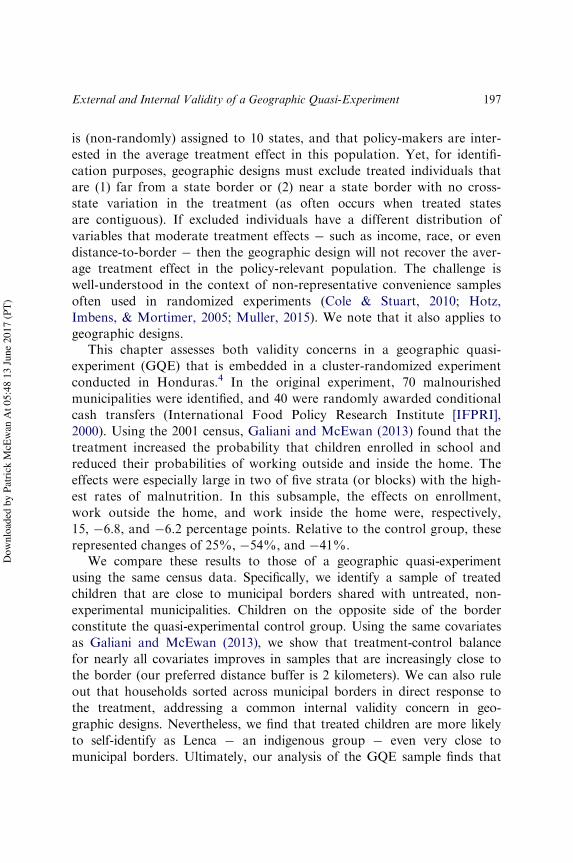
This chapter analyzes a geographic quasi-experiment embedded in acluster-randomized experiment in Honduras. In the experiment, averagetreatment effects of conditional cash transfers on school enrollment andchild labor were large ! especially in the poorest experimental blocks !and could be generalized to a policy-relevant population given the originalsample selection criteria. In contrast, the geographic quasi-experiment

Regression Discontinuity Designs: Theory and ApplicationsAdvances in Econometrics, Volume 38, 195!236Copyright r 2017 by Emerald Publishing LimitedAll rights of reproduction in any form reservedISSN: 0731-9053/doi:10.1108/S0731-905320170000038009

195

Dow

nloa

ded

by P

atric

k M

cEw

an A

t 05:

48 1

3 Ju

ne 2

017

(PT)

yielded point estimates that, for two of three dependent variables, wereattenuated. A judicious policy analyst without access to the experimentalresults might have provided misleading advice based on the magnitude ofpoint estimates. We assessed two main explanations for the difference inpoint estimates, related to external and internal validity.

Keywords: Geographical natural experiment; internal validity andexternal validity

1. INTRODUCTION

In a typical regression-discontinuity design, treatments are assigned on thebasis of a single, continuous covariate and a cutoff. The identification oftreatment effects relies on the assumption that the relation between potentialoutcomes and the assignment variable is continuous at the cutoff (Hahn,Todd, & van der Klaauw, 2001; Lee & Lemieux, 2010). The assumption isparticularly credible if a stochastic component in the assignment variable(e.g., a noisy test score) ensures that the agents cannot precisely manipulatetheir values of the assignment variable. That is, agents are subject to “local”random assignment (Lee, 2008; Lee & Lemieux, 2010).1

Researchers have extended the continuity results to regression-discon-tinuity designs in which assignment is based on a vector of variables(Imbens & Zajonc, 2009; Keele & Titiunik, 2015). A special case is the geo-graphic discontinuity design (GDD), in which exposure to a treatmentdepends on the latitude and longitude of agents with respect to an adminis-trative or territorial boundary. Researchers compare treated and untreatedagents residing near boundaries, using parametric and/or non-parametricmethods (Black, 1999; Dell, 2010; Keele & Titiunik, 2015). In the words ofLee and Lemieux (2010), these are often “nonrandomized” discontinuitydesigns since agents are usually aware of boundaries (and associated treat-ments) and can precisely choose their locations.2 This places a special bur-den on researchers to rule out location-based sorting on observed orunobserved variables as a threat to the internal validity of treatment effects(Keele, Lorch, Passarella, Small, & Titiunik, 2017; Keele & Titiunik, 2015,2016).

In addition to internal validity, one might assess the external validityof estimates obtained from geographic designs.3 Suppose that a treatment

196 SEBASTIAN GALIANI ET AL.

Dow

nloa

ded

by P

atric

k M

cEw

an A

t 05:

48 1

3 Ju

ne 2

017

(PT)

is (non-randomly) assigned to 10 states, and that policy-makers are inter-ested in the average treatment effect in this population. Yet, for identifi-cation purposes, geographic designs must exclude treated individuals thatare (1) far from a state border or (2) near a state border with no cross-state variation in the treatment (as often occurs when treated statesare contiguous). If excluded individuals have a different distribution ofvariables that moderate treatment effects ! such as income, race, or evendistance-to-border ! then the geographic design will not recover the aver-age treatment effect in the policy-relevant population. The challenge iswell-understood in the context of non-representative convenience samplesoften used in randomized experiments (Cole & Stuart, 2010; Hotz,Imbens, & Mortimer, 2005; Muller, 2015). We note that it also applies togeographic designs.

This chapter assesses both validity concerns in a geographic quasi-experiment (GQE) that is embedded in a cluster-randomized experimentconducted in Honduras.4 In the original experiment, 70 malnourishedmunicipalities were identified, and 40 were randomly awarded conditionalcash transfers (International Food Policy Research Institute [IFPRI],2000). Using the 2001 census, Galiani and McEwan (2013) found that thetreatment increased the probability that children enrolled in school andreduced their probabilities of working outside and inside the home. Theeffects were especially large in two of five strata (or blocks) with the high-est rates of malnutrition. In this subsample, the effects on enrollment,work outside the home, and work inside the home were, respectively,15, !6.8, and !6.2 percentage points. Relative to the control group, theserepresented changes of 25%, !54%, and !41%.

We compare these results to those of a geographic quasi-experimentusing the same census data. Specifically, we identify a sample of treatedchildren that are close to municipal borders shared with untreated, non-experimental municipalities. Children on the opposite side of the borderconstitute the quasi-experimental control group. Using the same covariatesas Galiani and McEwan (2013), we show that treatment-control balancefor nearly all covariates improves in samples that are increasingly close tothe border (our preferred distance buffer is 2 kilometers). We can also ruleout that households sorted across municipal borders in direct response tothe treatment, addressing a common internal validity concern in geo-graphic designs. Nevertheless, we find that treated children are more likelyto self-identify as Lenca ! an indigenous group ! even very close tomunicipal borders. Ultimately, our analysis of the GQE sample finds that

197External and Internal Validity of a Geographic Quasi-Experiment

Dow

nloa

ded

by P

atric

k M

cEw

an A

t 05:

48 1

3 Ju

ne 2

017

(PT)

point estimates for two of the three dependent variables are attenuatedrelative to the experimental benchmarks.

Is this because of imbalance in unobserved variables (i.e., a threat tointernal validity) or simply because the GQE sample has a different distribu-tion of observed or unobserved variables that moderate treatment effects?We separately assess each explanation using subsamples of the randomizedexperiment. First, we re-estimate experimental effects in the subsample oftreatment and control children within 2 kilometers of any municipal border(we refer to this as experiment 1). These estimates are slightly (but consis-tently) stronger than full-sample results. There are no mean differences incensus covariates between the two samples, suggesting that distance-to-border proxies unobserved moderators of treatment effects.

Second, we further restrict the sample in experiment 1 to treatment andcontrol children residing near the border of an untreated, non-experimentalmunicipality (we refer to this sample as experiment 2). Note that it includesexactly the same treated children as the GQE. However, it uses experimentalrather than the quasi-experimental controls. This permits us to (momentar-ily) abstract from internal validity. The point estimates for school enrollmentand work-in-home are attenuated relative to experiment 1. Descriptive sta-tistics suggests that the sample in experiment 2 is better-off than that ofexperiment 1, given higher rates of electricity use, asset ownership, and otherincome proxies. This plausibly explains the attenuated effects, since the liter-ature on conditional cash transfers finds smaller effects in when children areless poor (Fiszbein & Schady, 2009; Galiani & McEwan, 2013).

Third, we assess internal validity by comparing the unbiased estimatesfrom experiment 2 to those of the GQE (noting again that both include thesame treatment group but different control groups). Particularly for schoolenrollment, the GQE estimates are attenuated relative to those of experi-ment 2. It suggests that imbalance in unobserved variables results in down-ward biases in the GQE enrollment estimates. This is perhaps consistentwith the higher proportion of indigenous children in the GQE treatmentgroup, relative to its quasi-experimental control group.

In summary, we find that the GQE cannot fully replicate the policy-relevant experimental benchmark in Galiani and McEwan (2013) for rea-sons related to both validity concerns. Based on these results, we make twoconcrete recommendations. First, it is essential that researchers using a geo-graphic design carefully assess treatment-control balance on a wide rangeof observed covariates that are plausibly correlated with dependent vari-ables (echoing the recommendations of Keele et al., 2017). Our GQE is anespecially cautionary tale, since it had very good (but not perfect) balance

198 SEBASTIAN GALIANI ET AL.

Dow

nloa

ded

by P

atric

k M

cEw

an A

t 05:

48 1

3 Ju

ne 2

017

(PT)

in observed variables, but still could not replicate school enrollment esti-mates using the same treatment group and an experimental control group.

Second, we recommend that researchers assess the external validity oftheir geographic design by comparing the distributions of observed mod-erators of treatment effects ! such as household income ! to those of awell-defined, policy-relevant population. Aided by theory or prior empiri-cal evidence on the relevance of moderators, this can be used to specu-late about the generalizability of a GQE. More concretely, Cole andStuart (2010) describe how one might construct inverse-probabilityweights and re-weight a convenience sample ! whether experimental orquasi-experimental ! to resemble a well-defined population. We conductand report a similar analysis, re-weighting the sample of experiment 2 toresemble that of experiment 1. The weights are estimated using a widerange of covariates that are plausible moderators of treatment effects.Ultimately, however, the weighted estimates in experiment 2 are stillattenuated relative to experiment 1, suggesting that some relevant mod-erators are unobserved.

Our results contribute to a growing literature that compares regression-discontinuity designs with a single assignment variable to experimentalbenchmarks (see Shadish, Galindo, Wong, Steiner, & Cook, 2011 and thecitations therein). In this literature, several papers analyze conditional cashtransfer experiments in which eligibility was determined by a povertyproxy. Oosterbeek, Ponce, and Schady (2008) found that experimentalenrollment effects in Ecuador were large for the poorest households, butthat RDD effects were zero for less-poor households in the vicinity of theeligibility cutoff. Similarly, Galiani and McEwan (2013) found no effectson enrollment and child labor in the vicinity of the cutoff used to determineassignment to the experimental sample, but large experimental effectsamong households residing in municipalities with the lowest levels of theassignment variable. In the absence of an experiment, both papers cautionagainst generalizing “away” from cutoffs when the assignment variable is aplausible or well-documented moderator of treatment effects.5 A recentstrand of methodological literature has considered situations in which suchgeneralizations might still be possible.6

We first revisit the results from the original experiment in Galiani andMcEwan (2013), and then analyze the GQE sample and show that it failsto recover the experimental benchmark. Finally, we analyze experiments 1and 2 to assess the external and internal validity of the GQE to offer anexplanation for the divergence between the original experimental resultsand the results from the GQE.

199External and Internal Validity of a Geographic Quasi-Experiment

Dow

nloa

ded

by P

atric

k M

cEw

an A

t 05:

48 1

3 Ju

ne 2

017

(PT)

2. THE PRAF-II EXPERIMENT

2.1. Design and Treatment

In the late 1990s, the International Food Policy Research Institute (IFPRI)designed a cluster-randomized experiment to estimate the impact of condi-tional cash transfers (CCTs) on the poverty, education, and health out-comes of households in poor Honduran municipalities. In the absence of anational poverty map, researchers identified poor municipalities with anutrition-related proxy from a 1997 census of first-graders’ heights(Secretarıa de Educacion, 1997). IFPRI (2000) ordered 298 municipalitiesby their mean municipal height-for-age z-scores. Seventy-three municipali-ties with the lowest scores were eligible (the implied cutoff was !2.3,highlighting the extremely high rates of stunting). Three were excluded dueto accessibility, leaving an experimental sample of 70.

In 1999, IFPRI divided the sample into five quintiles of mean municipalheight-for-age. Within quintiles, municipalities were randomly assigned tothree treatment arms and a control group (in a ratio of 4:4:2:4). Arms 1and 2 received CCTs, while arms 2 and 3 were to receive grants to schoolsand health centers. Moore (2008) suggests the grants were sparsely imple-mented as late as 2002. Using this paper’s census data, Galiani andMcEwan (2013) failed to reject the null that average treatment effects inarms 1 and 2 were equal (relative to the control). Arm 3 had small and sta-tistically insignificant effects relative to the control (but its effect was statis-tically different from arm 2). Following Galiani and McEwan (2013), wecompare 40 municipalities in a pooled CCT treatment arm and 30 in apooled control group.

In the CCT treatment, households were eligible for an annual per-childcash transfer of L 800 (about US$50) if a child between 6 and 12 enrolledin primary school grades 1 to 4.7 Children with higher attainment were noteligible, and households could receive up to 3 per-child transfers. Duringthe experiment, transfers were distributed in November 2000, May!June2001, October 2001, and late 2002 (Galiani & McEwan, 2013; Morris,Flores, Olinto, & Medina, 2004). The average household in experimentalmunicipalities would have been eligible for transfers equal to about 5% ofmedian per capita expenditure (Galiani & McEwan, 2013). This is smallerthan most Latin American CCTs such as Progresa (Fiszbein & Schady,2009). Indeed, payments were only intended to cover the out-of-pocket andopportunity costs of enrolling a child in school (IFPRI, 2000).

200 SEBASTIAN GALIANI ET AL.

Dow

nloa

ded

by P

atric

k M

cEw

an A

t 05:

48 1

3 Ju

ne 2

017

(PT)

2.2. Data and Replication

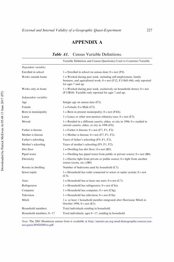
Galiani and McEwan (2013) used the 2001 Honduran census ! collectedin late July 2001 ! to estimate the short-run effects of offering CCTs toeligible children.8 Their sample contained 120,411 six to twelve year oldseligible for the education transfer, residing in the 70 experimental munici-palities. The census includes three dummy dependent variables: (1) whethera child was enrolled on the census date, (2) whether a child worked outsidethe home in the week preceding the census, and (3) whether a child workedexclusively in the home during the preceding week (Table A1 provides vari-able definitions).9

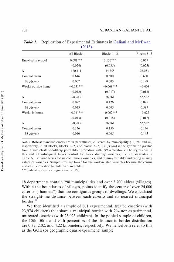
Their preferred specification regressed each dependent variable on atreatment dummy, dummy variables indicating randomization blocks, anda set of individual and household covariates unlikely to have been affectedby the treatment. Table 1 replicates the main results. The regressions in thisand subsequent tables control for block dummy variables, the 21 covariatesdescribed in Table A1, squared terms for continuous variables, and dummyvariables indicating missing values of any covariate. In addition to analyticstandard errors clustered by municipality, we report symmetric p-valuesfrom the wild cluster-bootstrap percentile-t that imposes the null hypothesis(Cameron, Gelbach, & Miller, 2008).

In the full sample, the treatment increases the probability of enrollmentby 8.1 percentage points (a 13% increase relative to the control group).The treatment reduces the probability of work outside the home by 3.1 p.p.(32%) and work only inside the home by 4.1 p.p. (30%). The effects arelarger in the two poorest blocks (1 and 2), and closer to zero and not statis-tically significant in three less-poor blocks (3, 4, and 5). In blocks 1 and 2,the effect on enrollment, work outside the home, and work inside the homeare, respectively, 15 p.p. (25%), !6.8 p.p. (!54%), and !6.2 p.p. (!41%).The magnitude of these effects is notable given the comparatively small sizeof the transfer.10

3. A GEOGRAPHIC QUASI-EXPERIMENT

3.1. Sample

The Honduran census does not record the precise location of dwellings. Toproxy location, we use the latitude and longitude of caserıos. In Honduras,

201External and Internal Validity of a Geographic Quasi-Experiment

Dow

nloa

ded

by P

atric

k M

cEw

an A

t 05:

48 1

3 Ju

ne 2

017

(PT)

18 departments contain 298 municipalities and over 3,700 aldeas (villages).Within the boundaries of villages, points identify the center of over 24,000caserıos (“hamlets”) that are contiguous groups of dwellings. We calculatedthe straight-line distance between each caserıo and its nearest municipalborder.11

We then identified a sample of 801 experimental, treated caserıos (with23,974 children) that share a municipal border with 794 non-experimental,untreated caserıos (with 25,025 children). In the pooled sample of children,the 10th, 50th, and 90th percentiles of the distance-to-border distributionare 0.37, 2.02, and 4.22 kilometers, respectively. We henceforth refer to thisas the GQE (or geographic quasi-experiment) sample.

Table 1. Replication of Experimental Estimates in Galiani and McEwan(2013).

All Blocks Blocks 1!2 Blocks 3!5

Enrolled in school 0.081*** 0.150*** 0.035

(0.024) (0.035) (0.025)

N 120,411 44,358 76,053

Control mean 0.646 0.600 0.680

BS p(sym) 0.007 0.005 0.198

Works outside home !0.031*** !0.068*** !0.008

(0.012) (0.017) (0.013)

N 98,783 36,261 62,522

Control mean 0.097 0.126 0.075

BS p(sym) 0.013 0.005 0.585

Works in home !0.041*** !0.062*** !0.027

(0.013) (0.018) (0.017)

N 98,783 36,261 62,522

Control mean 0.136 0.150 0.126

BS p(sym) 0.010 0.005 0.145

Notes: Robust standard errors are in parentheses, clustered by municipality (70, 28, and 42,respectively, in all blocks, blocks 1!2, and blocks 3!5). BS p(sym) is the symmetric p-valuefrom a wild cluster-bootstrap percentile-t procedure with 399 replications. The regressions inthis and all subsequent tables control for block dummy variables, the 21 covariates inTable A1, squared terms for six continuous variables, and dummy variables indicating missingvalues of variables. Sample sizes are lower for the work-related variables because the censusrestricts the question to children 7 and older.*** indicates statistical significance at 1%.

202 SEBASTIAN GALIANI ET AL.

Dow

nloa

ded

by P

atric

k M

cEw

an A

t 05:

48 1

3 Ju

ne 2

017

(PT)

The map in Fig. 1 illustrates the subsample of GQE caserıos that fallwithin 2 kilometers of a municipal border (in the next section, we provide arationale for using this distance buffer). It highlights that treated caserıosare a non-random sample of all treated caserıos. In particular, treatedcaserıos are excluded when their municipalities are fully circumscribed byother treatment or control municipalities in the experimental sample.

3.2. Covariate Balance Near Municipal Borders

By focusing on treated and untreated children that reside near municipalborders, there may be fewer differences in observed and, perhaps, unob-served variables that affect child outcomes. We assess this in the top-leftpanel of Fig. 2, using 21 covariates from the experimental analysis. Dots

Fig. 1. Caserıos in the Geographic Quasi-Experiment. Notes: Experimentaltreatment municipalities are lightly shaded; experimental control municipalities aredarkly shaded. Unshaded areas are untreated, non-experimental municipalities. Dotsindicate caserıos within 2 kilometers of municipal borders shared by experimentaltreatment municipalities and untreated non-experimental municipalities. The inset

map indicates department borders.

203External and Internal Validity of a Geographic Quasi-Experiment

Dow

nloa

ded

by P

atric

k M

cEw

an A

t 05:

48 1

3 Ju

ne 2

017

(PT)

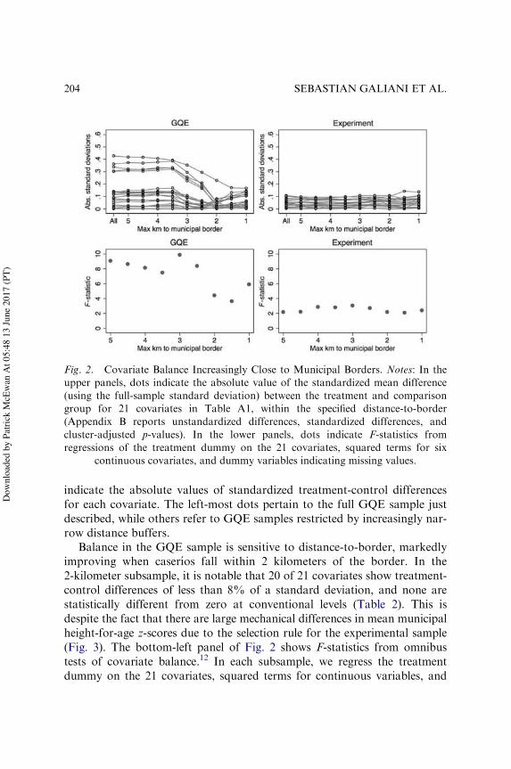
indicate the absolute values of standardized treatment-control differencesfor each covariate. The left-most dots pertain to the full GQE sample justdescribed, while others refer to GQE samples restricted by increasingly nar-row distance buffers.

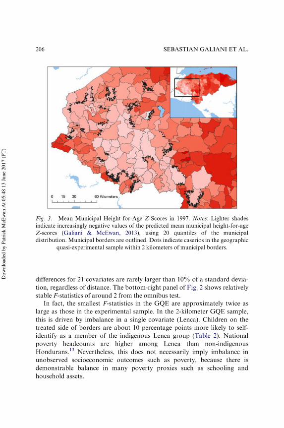
Balance in the GQE sample is sensitive to distance-to-border, markedlyimproving when caserıos fall within 2 kilometers of the border. In the2-kilometer subsample, it is notable that 20 of 21 covariates show treatment-control differences of less than 8% of a standard deviation, and none arestatistically different from zero at conventional levels (Table 2). This isdespite the fact that there are large mechanical differences in mean municipalheight-for-age z-scores due to the selection rule for the experimental sample(Fig. 3). The bottom-left panel of Fig. 2 shows F-statistics from omnibustests of covariate balance.12 In each subsample, we regress the treatmentdummy on the 21 covariates, squared terms for continuous variables, and

Fig. 2. Covariate Balance Increasingly Close to Municipal Borders. Notes: In theupper panels, dots indicate the absolute value of the standardized mean difference(using the full-sample standard deviation) between the treatment and comparisongroup for 21 covariates in Table A1, within the specified distance-to-border(Appendix B reports unstandardized differences, standardized differences, andcluster-adjusted p-values). In the lower panels, dots indicate F-statistics fromregressions of the treatment dummy on the 21 covariates, squared terms for six

continuous covariates, and dummy variables indicating missing values.

204 SEBASTIAN GALIANI ET AL.

Dow

nloa

ded

by P

atric

k M

cEw

an A

t 05:

48 1

3 Ju

ne 2

017

(PT)

dummies indicating missing values. The F-statistic declines as distance-to-border restrictions are applied, consistent with prior evidence.

In the right-hand panels of Fig. 2, we can compare balance in GQEsamples to balance in experimental samples with similar distance-to-borderrestrictions. As anticipated, given randomized assignment, covariate balancein the experiment does not depend on the distance of caserıos to municipalborders. The top-right panel shows that absolute values of treatment-control

Table 2. Balance in the Geographic Quasi-Experiment(≤2 kilometers from border).

T/C Differences p-Value

Age !0.002/!0.001 0.979

Female 0.007/0.013 0.383

Born in municipality !0.004/!0.013 0.849

Lenca 0.094/0.231 0.166

Moved 0.006/0.032 0.505

Father is literate 0.040/0.081 0.470

Mother is literate 0.030/0.060 0.531

Father’s schooling 0.231/0.076 0.689

Mother’s schooling 0.147/0.050 0.778

Dirt floor 0.008/0.017 0.915

Piped water 0.004/0.009 0.949

Electricity 0.022/0.053 0.827

Rooms in dwelling 0.041/0.054 0.747

Sewer/septic 0.030/0.063 0.683

Auto 0.006/0.029 0.780

Refrigerator !0.014/!0.051 0.791

Computer !0.001/!0.020 0.746

Television 0.012/0.035 0.890

Mitch !0.002/!0.009 0.890

Household members 0.054/0.022 0.692

Household members, 0!17 0.013/0.007 0.920

Predicted mean municipal child height-for-age z-score !0.464/!1.538 0.001

Note: In the difference column, the first number is the mean difference and the second numberis mean difference divided by the full-sample standard deviation. p-values account for cluster-ing by municipality.

205External and Internal Validity of a Geographic Quasi-Experiment

Dow

nloa

ded

by P

atric

k M

cEw

an A

t 05:

48 1

3 Ju

ne 2

017

(PT)

differences for 21 covariates are rarely larger than 10% of a standard devia-tion, regardless of distance. The bottom-right panel of Fig. 2 shows relativelystable F-statistics of around 2 from the omnibus test.

In fact, the smallest F-statistics in the GQE are approximately twice aslarge as those in the experimental sample. In the 2-kilometer GQE sample,this is driven by imbalance in a single covariate (Lenca). Children on thetreated side of borders are about 10 percentage points more likely to self-identify as a member of the indigenous Lenca group (Table 2). Nationalpoverty headcounts are higher among Lenca than non-indigenousHondurans.13 Nevertheless, this does not necessarily imply imbalance inunobserved socioeconomic outcomes such as poverty, because there isdemonstrable balance in many poverty proxies such as schooling andhousehold assets.

Fig. 3. Mean Municipal Height-for-Age Z-Scores in 1997. Notes: Lighter shadesindicate increasingly negative values of the predicted mean municipal height-for-ageZ-scores (Galiani & McEwan, 2013), using 20 quantiles of the municipaldistribution. Municipal borders are outlined. Dots indicate caserios in the geographic

quasi-experimental sample within 2 kilometers of municipal borders.

206 SEBASTIAN GALIANI ET AL.

Dow

nloa

ded

by P

atric

k M

cEw

an A

t 05:

48 1

3 Ju

ne 2

017

(PT)

3.3. Potential Threats to Internal Validity

Why might imbalance persist close to borders? One explanation is thatLenca households manipulated treatment status by moving after experi-mental assignment, but prior to the census. We regard this as unlikelyfor three reasons. First, the cash transfer for a typical household wasextremely small (less than 5% of a household’s consumption) andunlikely to provide sufficient liquidity for poor households to move.Second, 91% of children in the 2-kilometer GQE sample were born intheir municipality of residence, and only 4% lived in a different caserıo,aldea, or city in 1996 (five years before the census date). Both variablesare among those with the smallest cross-border differences in the GQE,and neither is statistically different from zero (Table 2).14 Third, there isa similar pattern of imbalance in the 2-kilometer sample of untreated,experimental caserıos that share a border with untreated, non-experimen-tal caserıos (see Table B2; we later use this sample to conduct a placebotest). In other words, imbalance persists even when there is no CCTtreatment to create incentives for cross-border sorting.

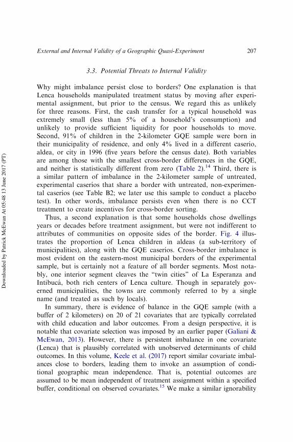
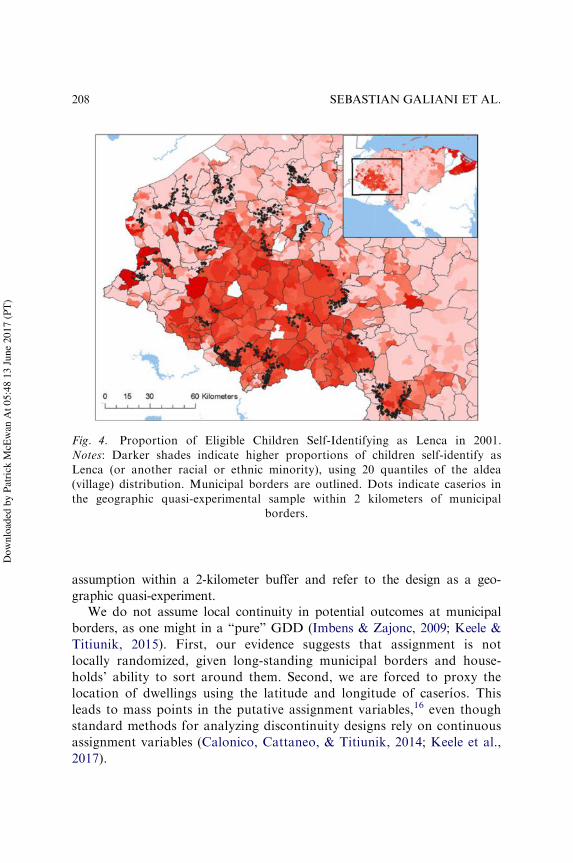
Thus, a second explanation is that some households chose dwellingsyears or decades before treatment assignment, but were not indifferent toattributes of communities on opposite sides of the border. Fig. 4 illus-trates the proportion of Lenca children in aldeas (a sub-territory ofmunicipalities), along with the GQE caserıos. Cross-border imbalance ismost evident on the eastern-most municipal borders of the experimentalsample, but is certainly not a feature of all border segments. Most nota-bly, one interior segment cleaves the “twin cities” of La Esperanza andIntibuca, both rich centers of Lenca culture. Though in separately gov-erned municipalities, the towns are commonly referred to by a singlename (and treated as such by locals).

In summary, there is evidence of balance in the GQE sample (with abuffer of 2 kilometers) on 20 of 21 covariates that are typically correlatedwith child education and labor outcomes. From a design perspective, it isnotable that covariate selection was imposed by an earlier paper (Galiani &McEwan, 2013). However, there is persistent imbalance in one covariate(Lenca) that is plausibly correlated with unobserved determinants of childoutcomes. In this volume, Keele et al. (2017) report similar covariate imbal-ances close to borders, leading them to invoke an assumption of condi-tional geographic mean independence. That is, potential outcomes areassumed to be mean independent of treatment assignment within a specifiedbuffer, conditional on observed covariates.15 We make a similar ignorability

207External and Internal Validity of a Geographic Quasi-Experiment

Dow

nloa

ded

by P

atric

k M

cEw

an A

t 05:

48 1

3 Ju

ne 2

017

(PT)

assumption within a 2-kilometer buffer and refer to the design as a geo-graphic quasi-experiment.

We do not assume local continuity in potential outcomes at municipalborders, as one might in a “pure” GDD (Imbens & Zajonc, 2009; Keele &Titiunik, 2015). First, our evidence suggests that assignment is notlocally randomized, given long-standing municipal borders and house-holds’ ability to sort around them. Second, we are forced to proxy thelocation of dwellings using the latitude and longitude of caserıos. Thisleads to mass points in the putative assignment variables,16 even thoughstandard methods for analyzing discontinuity designs rely on continuousassignment variables (Calonico, Cattaneo, & Titiunik, 2014; Keele et al.,2017).

Fig. 4. Proportion of Eligible Children Self-Identifying as Lenca in 2001.Notes: Darker shades indicate higher proportions of children self-identify asLenca (or another racial or ethnic minority), using 20 quantiles of the aldea(village) distribution. Municipal borders are outlined. Dots indicate caserios inthe geographic quasi-experimental sample within 2 kilometers of municipal

borders.

208 SEBASTIAN GALIANI ET AL.

Dow

nloa

ded

by P

atric

k M

cEw

an A

t 05:

48 1

3 Ju

ne 2

017

(PT)

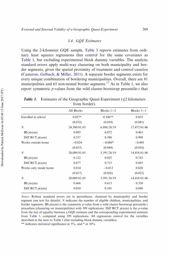
3.4. GQE Estimates

Using the 2-kilometer GQE sample, Table 3 reports estimates from ordi-nary least squares regressions that control for the same covariates asTable 1, but excluding experimental block dummy variables. The analyticstandard errors apply multi-way clustering on both municipality and bor-der segments, given the spatial proximity of treatment and control caserıos(Cameron, Gelbach, & Miller, 2011). A separate border segments exists forevery unique combination of bordering municipalities. Overall, there are 81municipalities and 65 non-nested border segments.17 As in Table 1, we alsoreport symmetric p-values from the wild cluster-bootstrap percentile-t that

Table 3. Estimates of the Geographic Quasi-Experiment (≤2 kilometersfrom border).

All Blocks Blocks 1!2 Blocks 3!5

Enrolled in school 0.057* 0.106** 0.035

(0.032) (0.054) (0.041)

N 24,360/81/65 6,888/26/19 17,472/61/46

BS p(sym) 0.095 0.072 0.463

Diff RCT p(sym) 0.537 0.580 0.998

Works outside home !0.024 !0.086* !0.005

(0.015) (0.044) (0.016)

N 20,009/81/65 5,591/26/19 14,418/61/46

BS p(sym) 0.122 0.025 0.743

Diff RCT p(sym) 0.677 0.715 0.885

Works only inside home 0.014 !0.013 0.026

(0.017) (0.026) (0.022)

N 20,009/81/65 5,591/26/19 14,418/61/46

BS p(sym) 0.468 0.613 0.330

Diff RCT p(sym) 0.010 0.105 0.048

Notes: Robust standard errors are in parentheses, clustered by municipality and bordersegment (see text for details). N indicates the number of eligible children, municipalities, andborder segments. BS p(sym) is the symmetric p-value from a wild cluster-bootstrap percentile-tprocedure (clustering on municipalities) with 399 replications. Diff RCT p(sym) is the p-valuefrom the test of equality between a GQE estimate and the corresponding experimental estimatefrom Table 1, computed using 399 replications. All regressions control for the variablesdescribed in the note to Table 1 (but excluding block dummy variables).** indicates statistical significance at 5%, and * at 10%.

209External and Internal Validity of a Geographic Quasi-Experiment

Dow

nloa

ded

by P

atric

k M

cEw

an A

t 05:

48 1

3 Ju

ne 2

017

(PT)

imposes the null hypothesis, clustering by municipality (Cameron et al.,2008).

In the 2-kilometer GQE sample, the treatment increases enrollment by amarginally significant 5.7 percentage points, or 2.4 p.p. smaller than theexperimental estimate in Table 1. In blocks 1!2, the enrollment effect is10.6 p.p., or 4.4 p.p. lower than the experimental estimate. In blocks 3!5,both the GQE and the experiment find similarly small and statisticallyinsignificant estimates.

The results are mixed for the two work-related variables. In the GQEsample, the treatment reduces work outside the home by 2.4 p.p. in allblocks and 8.6 p.p. in blocks 1!2 (only the latter is marginally statisticallysignificant). The experimental estimates are roughly similar. Neither theGQE nor the experiment suggest any effects in blocks 3!5. In contrast,the GQE estimates are attenuated for work inside the home, relative to theexperimental estimates. There is never a large or statistically significanteffect for this dependent variable in the GQE sample. Yet, in the experi-ment, there were reductions of 4.1 and 6.2 p.p., respectively, in all blocksand blocks 1!2.

Despite these differences between the GQE and the experiment, boot-strapped p-values in Table 3 suggest that the estimates are not statisticallydistinguishable from one another. Even so, one can pose a practical ques-tion: would a reasonable policy analyst ! relying on the GQE point esti-mates and blinded to the experimental ones ! have reached conclusions asoptimistic as those of Galiani and McEwan (2013)? Most likely the attenu-ated GQE estimates would have yielded more guarded conclusions.

4. EMPIRICAL STRATEGY

4.1. External and Internal Validity of the GQE

We consider two explanations for the divergence in point estimates of theGQE and the experiment, related to external and internal validity. Recallthat treated caserıos in the GQE are a non-random subset of all treatedcaserıos. First, they are close to municipal borders. Second, they share aborder with untreated, non-experimental caserıos. This naturally excludescaserıos in the spatial core of the experimental sample. As Figs. 3 and 4suggest, excluded caserıos might exhibit higher rates of child stunting orgreater concentrations of indigenous children.

210 SEBASTIAN GALIANI ET AL.

Dow

nloa

ded

by P

atric

k M

cEw

an A

t 05:

48 1

3 Ju

ne 2

017

(PT)

Thus, treated children in the GQE are plausibly different in variablesobserved by the econometrician ! such as distance-to-border, height-for-age, and ethnicity ! and perhaps in unobserved variables, such as income.If these variables moderate treatment effects, then the GQE estimates !even internally valid ones ! will differ from the experimental benchmarksin Table 1. In the present application, it is plausible that GQE caserıos are“less poor” than other treated ones. Since treatment effects are much largerin the poorest municipalities (Table 1), this provides a plausible explanationfor the attenuated GQE treatment effects.

An alternative explanation for the divergence of point estimates isrelated to internal validity. Suppose that treated children in the GQE differin unobserved ways from their bordering control group, even after condi-tioning on a rich set of covariates (e.g., they are more likely to be poor, anunmeasured variable). This too could explain attenuated treatment effects,assuming that poorer children are less likely to enroll in school and morelikely to work.

4.2. Experimental Samples Used to Assess Validity

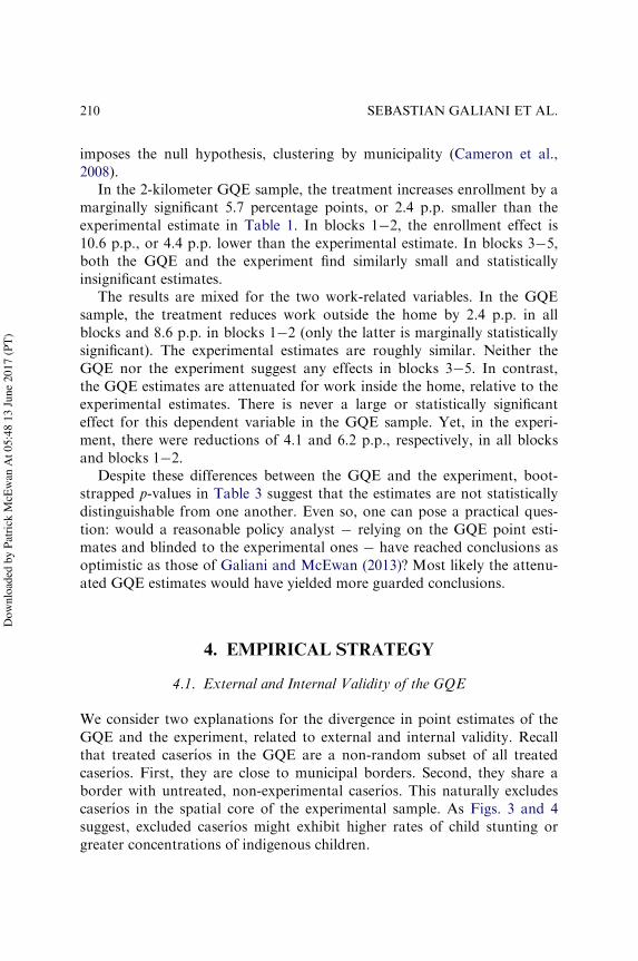
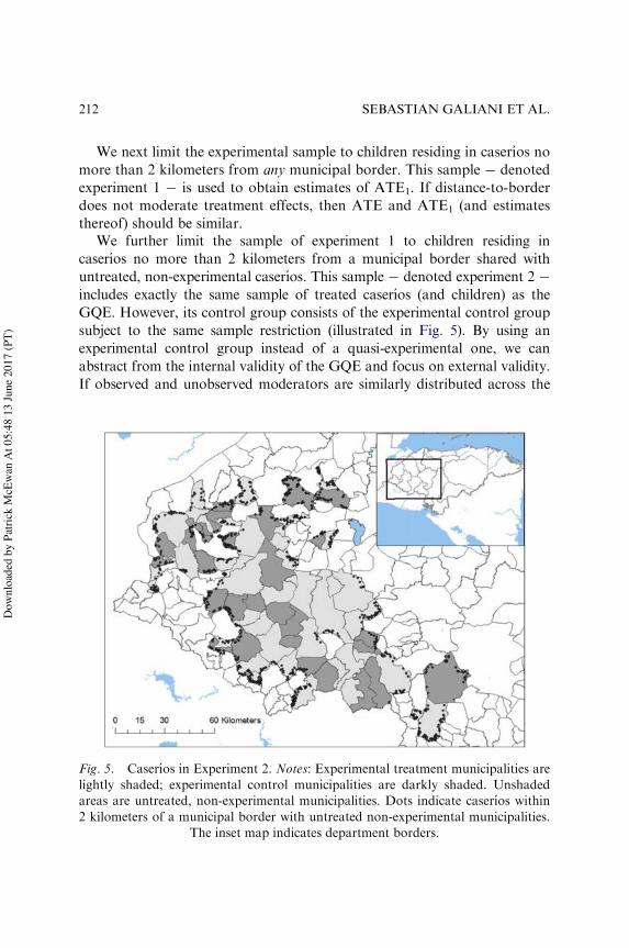
Table 4 summarizes the experimental samples that we use to assess theexternal and, then, the internal validity of the GQE. The full experimentalsample was already used, in Table 1, to obtain estimates of the averagetreatment effect (ATE). Given the design of the experiment, the estimatesare generalizable to a well-defined, policy-relevant population of Honduranchildren residing in malnourished municipalities.

Table 4. Experimental Samples Used to Assess External and InternalValidity of the GQE.

Sample Restriction on FullExperimental Sample

Parameter(s)

Full experimental sample ! ATE

Experiment 1 2 km from any municipal border ATE1

Experiment 2 2 km from municipal bordersshared with untreated, non-experimental caserıos

Unweighted: ATE2aWeighted: ATE1

Note: ATE is the average treatment effect in the full experimental sample (Galiani & McEwan,2013), and subscripts indicate average treatment effects in subsamples of the experiment.aIndicates that identification relies on a selection-on-observables assumption described in the text.

211External and Internal Validity of a Geographic Quasi-Experiment

Dow

nloa

ded

by P

atric

k M

cEw

an A

t 05:

48 1

3 Ju

ne 2

017

(PT)

We next limit the experimental sample to children residing in caserıos nomore than 2 kilometers from any municipal border. This sample ! denotedexperiment 1 ! is used to obtain estimates of ATE1. If distance-to-borderdoes not moderate treatment effects, then ATE and ATE1 (and estimatesthereof) should be similar.

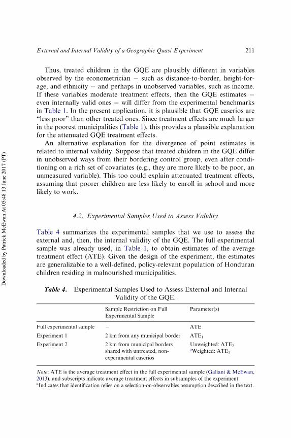
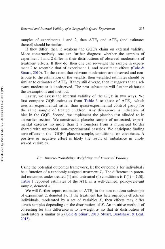
We further limit the sample of experiment 1 to children residing incaserıos no more than 2 kilometers from a municipal border shared withuntreated, non-experimental caserıos. This sample ! denoted experiment 2 !includes exactly the same sample of treated caserıos (and children) as theGQE. However, its control group consists of the experimental control groupsubject to the same sample restriction (illustrated in Fig. 5). By using anexperimental control group instead of a quasi-experimental one, we canabstract from the internal validity of the GQE and focus on external validity.If observed and unobserved moderators are similarly distributed across the

Fig. 5. Caserıos in Experiment 2. Notes: Experimental treatment municipalities arelightly shaded; experimental control municipalities are darkly shaded. Unshadedareas are untreated, non-experimental municipalities. Dots indicate caserıos within2 kilometers of a municipal border with untreated non-experimental municipalities.

The inset map indicates department borders.

212 SEBASTIAN GALIANI ET AL.

Dow

nloa

ded

by P

atric

k M

cEw

an A

t 05:

48 1

3 Ju

ne 2

017

(PT)

samples of experiments 1 and 2, then ATE1 and ATE2 (and estimatesthereof) should be similar.

If they differ, then it weakens the GQE’s claim on external validity.More constructively, one can further diagnose whether the samples ofexperiment 1 and 2 differ in their distributions of observed moderators oftreatment effects. If they do, then one can re-weight the sample in experi-ment 2 to resemble that of experiment 1, and re-estimate effects (Cole &Stuart, 2010). To the extent that relevant moderators are observed and con-tribute to the estimation of the weights, then weighted estimates should besimilar to estimates of ATE1. If they still diverge, then it suggests that a rel-evant moderator is unobserved. The next subsection will further elaboratethe assumptions and method.

Lastly, we assess the internal validity of the GQE in two ways. Wefirst compare GQE estimates from Table 3 to those of ATE2, whichuses an experimental rather than quasi-experimental control group forthe same sample of treated children. Any divergence is indicative ofbias in the GQE. Second, we implement the placebo test alluded to inan earlier section. We construct a placebo sample of untreated, experi-mental caserıos no more than 2 kilometers from a municipal bordershared with untreated, non-experimental caserıos. We anticipate findingzero effects in the “GQE” placebo sample, conditional on covariates. Apositive or negative effect is likely the result of imbalance in unob-served variables.

4.3. Inverse-Probability Weighting and External Validity

Using the potential outcomes framework, let the outcome Y for individual ibe a function of a randomly assigned treatment Ti. The difference in poten-tial outcomes under treated (1) and untreated (0) conditions is Yi 1ð Þ ! Yi 0ð Þ.Table 1 reported estimates of the ATE in a well-defined, policy-relevantsample, denoted S.

We will further report estimates of ATE2 in the non-random subsampleof experiment 2, denoted S2. If the treatment has heterogeneous effects onindividuals, moderated by a set of variables X, then effects may differacross samples depending on the distribution of X. An intuitive method ofcorrecting for this difference is to re-weight S2 so that its distribution ofmoderators is similar to S (Cole & Stuart, 2010; Stuart, Bradshaw, & Leaf,2015).

213External and Internal Validity of a Geographic Quasi-Experiment

Dow

nloa

ded

by P

atric

k M

cEw

an A

t 05:

48 1

3 Ju

ne 2

017

(PT)

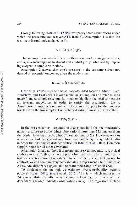
Closely following Hotz et al. (2005), we specify three assumptions underwhich the procedure can recover ATE from S2. Assumption 1 is that thetreatment is randomly assigned in S2:

Ti ⊥ [Yi 1ð Þ; Yi 0ð Þ]jS2:

The assumption is satisfied because there was random assignment in S,and S2 is a subsample of treatment and control groups obtained by impos-ing exogenous sample restrictions.

Assumption 2 asserts that one’s presence in the subsample does notdepend on potential outcomes, given the moderators:

i∈ S2ð Þ ⊥ [Yi 1ð Þ;Yi 0ð Þ]jXi:

Hotz et al. (2005) refer to this as unconfounded location. Stuart, Cole,Bradshaw, and Leaf (2011) invoke a similar assumption and refer to it asunconfounded sample selection. Both papers highlight the need to measureall relevant moderators in order to satisfy the assumption. Lastly,Assumption 3 imposes a requirement of common support for the modera-tors between the two samples. For each moderator, it must be the case that:

0<P i∈ S2jXið Þ< 1:

In the present context, assumption 3 does not hold for one moderator,namely distance-to-border (since observations more than 2 kilometers fromthe border have zero probability of contributing to S2). However, we canreframe the task as generalizing from the sample S2 to S1, which alsoimposes the 2-kilometer distance restriction (Stuart et al., 2011). Commonsupport holds for all other covariates.

Assumption 2 may not hold if there are unobserved moderators. A typicalstudy cannot verify this, just as a typical observational study cannot directlytest for selection-on-unobservables into a treatment or control group. Incontrast, we can compare weighted estimates in experiment 2 to estimates ofATE1. Any difference suggests that relevant moderators are unobserved.

To implement the method, we estimate inverse-probability weights(Cole & Stuart, 2010; Stuart et al., 2015).18 In S1 ! which imposes the2-kilometer distance buffer ! we estimate a logit regression in which thedependent variable indicates observations in S2. The regressors include

214 SEBASTIAN GALIANI ET AL.

Dow

nloa

ded

by P

atric

k M

cEw

an A

t 05:

48 1

3 Ju

ne 2

017

(PT)

21 covariates, 6 squared terms, and dummy variables indicating missingvalues.19 They further include block dummy variables, mean municipalheight-for-age, distance-to-border, and squared terms for the latter two.Lastly, we calculate inverse-probability weights for observations in S2 aswiðXiÞ ¼ 1=pðXiÞ, where p is the estimated probability that an observationis selected for S2.

5. RESULTS

5.1. External Validity: Experiment 1

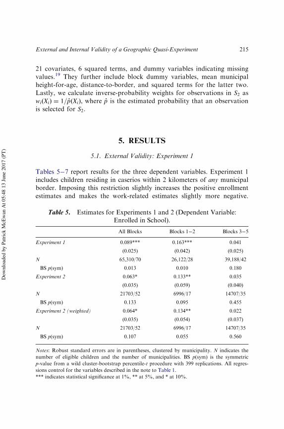
Tables 5!7 report results for the three dependent variables. Experiment 1includes children residing in caserıos within 2 kilometers of any municipalborder. Imposing this restriction slightly increases the positive enrollmentestimates and makes the work-related estimates slightly more negative.

Table 5. Estimates for Experiments 1 and 2 (Dependent Variable:Enrolled in School).

All Blocks Blocks 1!2 Blocks 3!5

Experiment 1 0.089*** 0.163*** 0.041

(0.025) (0.042) (0.025)

N 65,310/70 26,122/28 39,188/42

BS p(sym) 0.013 0.010 0.180

Experiment 2 0.063* 0.133** 0.035

(0.035) (0.059) (0.040)

N 21703/52 6996/17 14707/35

BS p(sym) 0.133 0.095 0.455

Experiment 2 (weighted) 0.064* 0.134** 0.022

(0.035) (0.054) (0.037)

N 21703/52 6996/17 14707/35

BS p(sym) 0.107 0.055 0.560

Notes: Robust standard errors are in parentheses, clustered by municipality. N indicates thenumber of eligible children and the number of municipalities. BS p(sym) is the symmetricp-value from a wild cluster-bootstrap percentile-t procedure with 399 replications. All regres-sions control for the variables described in the note to Table 1.*** indicates statistical significance at 1%, ** at 5%, and * at 10%.

215External and Internal Validity of a Geographic Quasi-Experiment

Dow

nloa

ded

by P

atric

k M

cEw

an A

t 05:

48 1

3 Ju

ne 2

017

(PT)

In Table 5, for example, the enrollment estimate is 8.9 percentage pointsinside the buffer (vs. 8.1 in Table 1). Further limiting the sample to blocks1 and 2, the estimate in experiment 1 is 16.3 p.p. (vs. 15 p.p. in Table 1).There is no ready explanation for the slight increases in enrollment effectsin Table 5 (and slightly more negative work effects reported in Tables 6and 7). The mean covariate differences between the full experimental sam-ple and experiment 1 are small and statistically insignificant (full results areavailable from the authors). This suggests that distance-to-border is aproxy for other, unobserved moderators.

5.2. External Validity: Experiment 2

Tables 5!7 also report estimates for experiment 2. Recall that it includesthe same treated observations as the GQE sample, but with an experimen-tal control group. Imposing this sample restriction reduces the enrollmentestimates by 2.6 p.p. relative to experiment 1, apparently driven by a 3 p.p.

Table 6. Estimates for Experiments 1 and 2 (Dependent Variable: WorksOutside Home).

All Blocks Blocks 1!2 Blocks 3!5

Experiment 1 !0.042*** !0.082*** !0.017

(0.012) (0.022) (0.012)

N 53,703/70 21,387/28 32,316/42

BS p(sym) 0.003 0.003 0.217

Experiment 2 !0.032* !0.090** !0.009

(0.017) (0.034) (0.017)

N 17,883/52 5,691/17 12,192/35

BS p(sym) 0.095 0.013 0.632

Experiment 2 (weighted) !0.034* !0.087** !0.009

(0.017) (0.033) (0.018)

N 17,883/52 5,691/17 12,192/35

BS p(sym) 0.070 0.007 0.637

Notes: Robust standard errors are in parentheses, clustered by municipality. N indicates thenumber of eligible children and the number of municipalities. BS p(sym) is the symmetricp-value from a wild cluster-bootstrap percentile-t procedure with 399 replications. All regres-sions control for the variables described in the note to Table 1.*** indicates statistical significance at 1%, ** at 5%, and * at 10%.

216 SEBASTIAN GALIANI ET AL.

Dow

nloa

ded

by P

atric

k M

cEw

an A

t 05:

48 1

3 Ju

ne 2

017

(PT)

decline in the blocks 1!2 subsample. A similar pattern of attenuation isevident for work-in-home estimates (Table 7), but not for work-outside-home (Table 6). For the latter variable, the coefficient in the blocks 1!2sample is slightly more negative.

Did the sample restriction in experiment 2 change the distribution ofplausible moderating variables? In fact, observations in the experiment 2sample are 8 percentage points less likely to belong to blocks 1!2(Table C1). There are also substantial differences for specific covariates,especially within blocks 1!2 (Fig. 6). For example, households of childrenin experiment 2 are 12 p.p. more likely to have electric light, 10 p.p. morelikely to own a television, and their mothers have two-thirds of a year moreschooling, on average. In addition to Galiani and McEwan (2013), the liter-ature on Latin American CCTs usually finds that effects on school enroll-ment are larger among poorer households (Fiszbein & Schady, 2009). Thisimplies that sample selection on observed (and perhaps unobserved) moder-ating variables ! all common proxies for poverty ! is responsible for thepattern of attenuated estimates in experiment 2.

Table 7. Estimates for Experiments 1 and 2 (Dependent Variable: WorksOnly in Home).

All Blocks Blocks 1!2 Blocks 3!5

Experiment 1 !0.041*** !0.067*** !0.024

(0.013) (0.021) (0.016)

N 53,703/70 21,387/28 32,316/42

BS p(sym) 0.007 0.025 0.188

Experiment 2 !0.024 !0.026 !0.023

(0.019) (0.025) (0.023)

N 17,883/52 5,691/17 12,192/35

BS p(sym) 0.320 0.352 0.448

Experiment 2 (weighted) !0.018 !0.020 !0.013

(0.019) (0.025) (0.022)

N 17,883/52 5,691/17 12,192/35

BS p(sym) 0.438 0.515 0.630

Notes: Robust standard errors are in parentheses, clustered by municipality. N indicates thenumber of eligible children and the number of municipalities. BS p(sym) is the symmetricp-value from a wild cluster-bootstrap percentile-t procedure with 399 replications. All regres-sions control for the variables described in the note to Table 1.*** indicates statistical significance at 1%.

217External and Internal Validity of a Geographic Quasi-Experiment

Dow

nloa

ded

by P

atric

k M

cEw

an A

t 05:

48 1

3 Ju

ne 2

017

(PT)

5.3. External Validity: Weighted Estimates in Experiment 2

To further examine this issue, we estimated the probability that each obser-vation in experiment 1 was selected for experiment 2 (using the logit specifi-cation described earlier). The mean difference in the estimated propensityscore between the samples of experiment 2 and experiment 1 is 0.045 (or37% of the standard deviation in the experiment 1 sample). For each of the21 covariates, we then estimated the standardized difference between theweighted mean in experiment 2 ! applying the inverse-probability weightsdescribed earlier ! and the unweighted mean in experiment 1. As Fig. 6illustrates, re-weighting nearly eliminates observed differences between thetwo samples.

Finally, Tables 5!7 report weighted estimates in the experiment 2 sam-ple. We anticipate that the weighted estimates will more closely resemblethose from experiment 1. On the contrary, we find that the point estimates

Fig. 6. Comparing Covariate Means between Samples in Experiments 1 and 2.Notes: Dots indicate the absolute value of the standardized mean difference (usingthe full-sample standard deviation) between the pooled experiment 2 sample andthe pooled experiment 1 sample, for the 21 covariates in Table A1. In all panels, thesample includes caserıos within 2 kilometers of municipal borders. In the rightpanel, the mean of the experiment 2 sample is weighted, as described in the text.

218 SEBASTIAN GALIANI ET AL.

Dow

nloa

ded

by P

atric

k M

cEw

an A

t 05:

48 1

3 Ju

ne 2

017

(PT)

from unweighted and weighted specifications in experiment 2 are quite simi-lar (and both exhibit similar patterns of attenuation relative to experiment 1).One interpretation is that sample selection into experiment 2 altered the dis-tribution of unobserved variables that moderate treatment effects, leading toa violation of assumption 2.

What else might be done? One possibility is to implement a two-stagecorrection for sample selection, a la Heckman (1979). In the sample ofexperiment 1, one estimates a first-stage probit with a dependent variableindicating selection into experiment 2. It includes the same independentvariables as the logit used to estimate the inverse-probability weights, inaddition to variables that affects selection into experiment 1, but not childoutcomes. Of course, compelling exclusion restrictions are usually hard tocome by (and no obvious candidates exist in our application). Finally, inthe second-stage regression, one includes the inverse Mills ratio as a regres-sor (along with other covariates) and examines its sign and significance forevidence of sample selection bias.

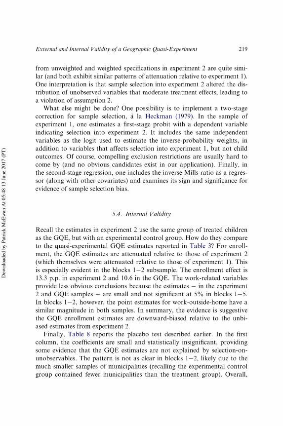
5.4. Internal Validity

Recall the estimates in experiment 2 use the same group of treated childrenas the GQE, but with an experimental control group. How do they compareto the quasi-experimental GQE estimates reported in Table 3? For enroll-ment, the GQE estimates are attenuated relative to those of experiment 2(which themselves were attenuated relative to those of experiment 1). Thisis especially evident in the blocks 1!2 subsample. The enrollment effect is13.3 p.p. in experiment 2 and 10.6 in the GQE. The work-related variablesprovide less obvious conclusions because the estimates ! in the experiment2 and GQE samples ! are small and not significant at 5% in blocks 1!5.In blocks 1!2, however, the point estimates for work-outside-home have asimilar magnitude in both samples. In summary, the evidence is suggestivethe GQE enrollment estimates are downward-biased relative to the unbi-ased estimates from experiment 2.

Finally, Table 8 reports the placebo test described earlier. In the firstcolumn, the coefficients are small and statistically insignificant, providingsome evidence that the GQE estimates are not explained by selection-on-unobservables. The pattern is not as clear in blocks 1!2, likely due to themuch smaller samples of municipalities (recalling the experimental controlgroup contained fewer municipalities than the treatment group). Overall,

219External and Internal Validity of a Geographic Quasi-Experiment

Dow

nloa

ded

by P

atric

k M

cEw

an A

t 05:

48 1

3 Ju

ne 2

017

(PT)

the imprecision prevents us from ruling out some bias in the GQEestimates.

5.5. Compound Treatment Irrelevance

The GQE must assume that the CCT is the only treatment that variesacross borders (or, if there is another that does not affect potential out-comes). Keele and Titiunik (2015, 2016) describe this assumption as com-pound treatment irrelevance. In the Honduran context, the most likelyviolation occurs when a municipal border is also a department border.Although the management and financing of Honduran public schools isstill highly centralized, each department controls some functions, especiallyrelated to personnel management. This leaves open the possibility that theassumption is violated, and so we assess robustness to the dropping ofobservations near municipal border segments that also happen to bedepartment borders.

Table 8. Placebo Estimates (≤ 2 kilometers from border).

All Blocks Blocks 1!2 Blocks 3!5

Enrolled in school !0.025 0.073 !0.052

(0.036) (0.063) (0.035)

N 13,980/47/40 4,064/17/12 9,916/33/28

BS p(sym) 0.525 0.415 0.165

Works outside home !0.014 !0.035 !0.008

(0.018) (0.054) (0.015)

N 11,573/47/40 3,365/17/12 8,208/33/28

BS p(sym) 0.542 0.705 0.623

Works only inside home !0.001 !0.069** 0.024

(0.019) (0.032) (0.018)

N 11,573/47/40 3,365/17/12 8,208/33/28

BS p(sym) 0.930 0.135 0.188

Notes: Robust standard errors are in parentheses, clustered by municipality and bordersegment (see text for details). N indicates the number of eligible children, municipalities, andborder segments. BS p(sym) is the symmetric p-value from a wild cluster-bootstrap percentile-tprocedure (clustering on municipalities) with 399 replications. All regressions control for thevariables described in the note to Table 1 (but excluding block dummy variables).**indicates statistical significance at 5%.

220 SEBASTIAN GALIANI ET AL.

Dow

nloa

ded

by P

atric

k M

cEw

an A

t 05:

48 1

3 Ju

ne 2

017

(PT)

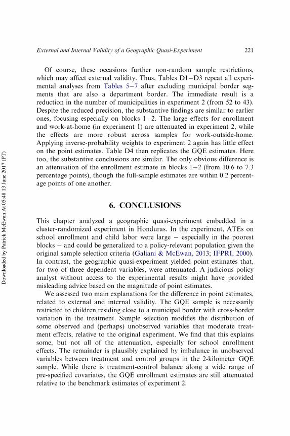
Of course, these occasions further non-random sample restrictions,which may affect external validity. Thus, Tables D1!D3 repeat all experi-mental analyses from Tables 5!7 after excluding municipal border seg-ments that are also a department border. The immediate result is areduction in the number of municipalities in experiment 2 (from 52 to 43).Despite the reduced precision, the substantive findings are similar to earlierones, focusing especially on blocks 1!2. The large effects for enrollmentand work-at-home (in experiment 1) are attenuated in experiment 2, whilethe effects are more robust across samples for work-outside-home.Applying inverse-probability weights to experiment 2 again has little effecton the point estimates. Table D4 then replicates the GQE estimates. Heretoo, the substantive conclusions are similar. The only obvious difference isan attenuation of the enrollment estimate in blocks 1!2 (from 10.6 to 7.3percentage points), though the full-sample estimates are within 0.2 percent-age points of one another.

6. CONCLUSIONS

This chapter analyzed a geographic quasi-experiment embedded in acluster-randomized experiment in Honduras. In the experiment, ATEs onschool enrollment and child labor were large ! especially in the poorestblocks ! and could be generalized to a policy-relevant population given theoriginal sample selection criteria (Galiani & McEwan, 2013; IFPRI, 2000).In contrast, the geographic quasi-experiment yielded point estimates that,for two of three dependent variables, were attenuated. A judicious policyanalyst without access to the experimental results might have providedmisleading advice based on the magnitude of point estimates.

We assessed two main explanations for the difference in point estimates,related to external and internal validity. The GQE sample is necessarilyrestricted to children residing close to a municipal border with cross-bordervariation in the treatment. Sample selection modifies the distribution ofsome observed and (perhaps) unobserved variables that moderate treat-ment effects, relative to the original experiment. We find that this explainssome, but not all of the attenuation, especially for school enrollmenteffects. The remainder is plausibly explained by imbalance in unobservedvariables between treatment and control groups in the 2-kilometer GQEsample. While there is treatment-control balance along a wide range ofpre-specified covariates, the GQE enrollment estimates are still attenuatedrelative to the benchmark estimates of experiment 2.

221External and Internal Validity of a Geographic Quasi-Experiment

Dow

nloa

ded

by P

atric

k M

cEw

an A

t 05:

48 1

3 Ju

ne 2

017

(PT)

Both findings suggest that researchers using geographic designs shouldcarefully describe how their geographically imposed convenience sample dif-fers from that of a well-defined, policy-relevant population. If feasible, theymight further apply inverse-probability weighting as a robustness check(following Cole & Stuart, 2010 and the analysis herein). Moreover, theyshould carefully assess treatment-control balance in the geographic sample.In this volume, Keele et al. (2017) discuss related consideration when unitsof analysis (such as households) cannot be precisely geo-located.

The findings on external validity have broader implications for thedesign and interpretation of randomized field experiments, which often relyon convenience samples defined by observed and unobserved moderatorsof treatment effects (such as poverty, distance to urban centers, agents’willingness to submit to randomization). At a minimum, experimentsshould specifically describe the criteria for sample selection (Campbell,Piaggio, Elbourne, & Altman, 2012), and whether these variables are plau-sible moderators of treatment effects. Our chapter suggests that authorscan push this exercise further and assess robustness after re-weighting theexperimental convenience sample to resemble a policy-relevant population,with appropriate caveats about selection-on-unobservables into the conve-nience sample (Cole & Stuart, 2010; Hotz et al., 2005; Stuart et al., 2015).

NOTES

1. Cattaneo, Frandsen, and Titiunik (2015) push this interpretation further byimplementing randomization inference in samples near the cutoff.

2. In rare cases, boundaries might be suddenly (and quasi-randomly) redrawn,leading to a more credible “re-randomization” of households before endogenoussorting begins anew (Billings, Deming, & Rockoff, 2013).

3. External validity exists when causal relationships “[hold] over variations in per-sons, settings, treatment variables, and measurement variables” (Shadish, Cook, &Campbell, 2002, p. 507). Some authors assess the importance of variation in treat-ments (particularly implementer characteristics) and measurement variables (Allcott,2015; Bold et al., 2013; Lucas, McEwan, Ngware, & Oketch, 2014). This paperfocuses on the potentially moderating role of independent variables related to personsand settings.

4. We refer to it as a geographic quasi-experiment because assignment is nottransparently random (even local to borders), and because we must proxy the loca-tion of children using the coordinates of their caserıo (a cluster of dwellings). Thelatter introduces mass points in the putative assignment variables of latitude andlongitude in a geographic discontinuity design. For related explanations, see Keeleet al. (2016) and later sections of this paper.

222 SEBASTIAN GALIANI ET AL.

Dow

nloa

ded

by P

atric

k M

cEw

an A

t 05:

48 1

3 Ju

ne 2

017

(PT)

5. Buddelmeyer and Skoufias (2004) analyzed Mexico’s well-known Progresaexperiment (and a proxy means test and cutoff used to determine eligibility). In con-trast to other results, they found that experimental enrollment estimates in samples“close” to the eligibility cutoff were roughly similar or slightly larger than full-sampleestimates.

6. Angrist and Rokkanen (2015) show how RDD effects might be estimated“away” from the cutoff if the assignment variable is ignorable, conditional on a setof covariates unaffected by the treatment. Dong and Lewbel (2015) note that therelative slopes of lines fit to data within bandwidths on either side of the cutoff pro-vide insights into how modest changes in the assignment cutoff could affect themagnitude of estimated effects.

7. A school attendance condition was apparently not enforced (Glewwe &Olinto, 2004).

8. A related literature uses a panel household survey ! collected in 2000 and2002 ! to estimate effects on child health and nutrition (Morris et al., 2004), educa-tion (Glewwe & Olinto, 2004), and adult labor supply (Alzua, Cruces, & Ripani,2013).

9. The interpretation of work-only-inside-home variable is governed by the flowof survey questions.10. Benedetti, Ibarraran, and McEwan (2016) analyze a later Honduran CCT

experiment ! also conducted in a sample of poor municipalities ! which offeredmuch larger transfers. They found smaller effects on both enrollment and childlabor, which they attributed to a weaker application of the education enrollmentcondition.11. We identified the caserıo coordinates for 93% of all 6!12 year olds in the

census (and 95% of the full experimental sample). The missing coordinates are dueto incomplete geocoding of caserıos in an ArcGIS file obtained from theInfotecnologıa unit of the Secretarıa de Educacion in 2008.12. A simulation in Hansen and Bowers (2008) shows that a similar test using

logistic regression leads to over-rejection of the null with a modest number ofassigned units (100). In the present case, we are concerned with comparing balanceacross subsamples.13. In a national sample from 2004, the poverty headcount is 49% among non-

indigenous individuals and 71% among ethnic and racial minorities (World Bank,2006).14. It is possible that households somehow misreported their answers, but seems

unlikely given the fact that census data collection was independent of PRAF,IFPRI, and the original impact evaluation’s data collection schedule.15. The standardized differences are within thresholds beyond which regression

adjustment is particularly sensitive to specification (Imbens & Wooldridge, 2009;Rubin, 2001).16. In a histogram of distance-to-border distribution in the GQE sample ! avail-

able from the authors ! there is a puzzlingly large spike on the untreated side of theborder, between 3 and 4 kilometers away. In fact, this is the town of Santa Barbara(identified as a single caserıo in Honduran data). It stretches about 2 kilometersacross at its widest point and contains 1,178 dwellings with eligible children. If dis-tance-to-border had been measured without error for each dwelling, it might have

223External and Internal Validity of a Geographic Quasi-Experiment

Dow

nloa

ded

by P

atric

k M

cEw

an A

t 05:

48 1

3 Ju

ne 2

017

(PT)

“filled” an apparent notch in the histogram. This is the most severe example in theGQE sample of mis-measurement of the assignment variable, given the use ofcaserıo rather than dwelling location. In the full GQE sample of caserıos, the mean(median) number of dwellings is 16.6 (8), and the 90th and 95th percentiles are 33and 47, respectively.17. When GQE estimates are reported within subsamples of blocks 1!2 and

3!5, control observations in untreated, non-experimental municipalities areassigned to the block corresponding to the treated observations on the opposite sideof the border segment.18. Cole and Stuart (2011) prove that the method yields consistent estimates ! in

this paper, of ATE1 ! under assumptions similar to those just described.19. When weighted estimates are reported in subsamples (e.g., blocks 1!2), we

separately estimate weights in that subsample.

ACKNOWLEDGMENTS

We are grateful to Matias Cattaneo, Juan Carlos Escanciano, Luke Keele,Rocıo Titiunik, the anonymous referees, and participants of the Advancesin Econometrics conference at the University of Michigan for their helpfulcomments, without implicating them for errors or interpretations.

REFERENCES

Allcott, H. (2015). Site selection bias in program evaluation. The Quarterly Journal ofEconomics, 130(3), 1117!1165. doi:10.1093/qje/qjv015

Alzua, M. L., Cruces, G., & Ripani, L. (2013). Welfare programs and labor supply in develop-ing countries: Experimental evidence from Latin America. Journal of PopulationEconomics, 26(4), 1255!1284. doi:10.1007/s00148-012-0458-0

Angrist, J. D., & Rokkanen, M. (2015). Wanna get away? Regression discontinuity estimationof exam school effects away from the cutoff. Journal of the American StatisticalAssociation, 110, 1331!1344.

Benedetti, F., Ibarraran, P., & McEwan, P. J. (2016). Do education and health conditions mat-ter in a large cash transfer? Evidence from a Honduran experiment. EconomicDevelopment and Cultural Change. doi:10.1086/686583

Billings, S. B., Deming, D. J., & Rockoff, J. (2013). School segregation, educational attain-ment, and crime: Evidence from the end of busing in Charlotte-Mecklenburg. TheQuarterly Journal of Economics, 129(1), 435!476. doi:10.1093/qje/qjt026

Black, S. (1999). Do better schools matter? Parental valuation of elementary education.Quarterly Journal of Economics, 114, 577!599.

Bold, T., Kimenyi, M., Mwabu, G., Ng’ang’a, A., & Sandefur, J. (2013). Scaling-up whatworks: Experimental evidence on external validity in Kenyan Education. Centre for theStudy of African Economies WPS/2013-04.

224 SEBASTIAN GALIANI ET AL.

Dow

nloa

ded

by P

atric

k M

cEw

an A

t 05:

48 1

3 Ju

ne 2

017

(PT)

Buddelmeyer, H., & Skoufias, E. (2004). An evaluation of the performance of regression dis-continuity design on PROGRESA. Policy Research Working Paper No. 3386. WorldBank, Washington, DC.

Calonico, S., Cattaneo, M. D., & Titiunik, R. (2014). Robust nonparametric confidence inter-vals for regression-discontinuity designs. Econometrica, 82(6), 2295!2326. doi:10.3982/ecta11757

Cameron, A. C., Gelbach, J. B., & Miller, D. L. (2008). Bootstrap-based improvements forinference with clustered errors. Review of Economics and Statistics, 90(3), 414!427.doi:10.1162/rest.90.3.414

Cameron, A. C., Gelbach, J. B., & Miller, D. L. (2011). Robust inference with multiway clustering.Journal of Business &Economic Statistics, 29(2), 238!249. doi:10.1198/jbes.2010.07136

Campbell, M. K., Piaggio, G., Elbourne, D. R., & Altman, D. G. (2012). Consort 2010 state-ment: Extension to cluster randomised trials. BMJ, 345, e5661. doi:10.1136/bmj.e5661

Cattaneo, M. D., Frandsen, B. R., & Titiunik, R. (2015). Randomization inference in theregression discontinuity design: An application to party advantages in the U.S. Senate.Journal of Causal Inference, 3(1), 1!24. doi:10.1515/jci-2013-0010

Cole, S. R., & Stuart, E. A. (2010). Generalizing evidence from randomized clinical trials totarget populations: The ACTG 320 trial. American Journal of Epidemiology, 172(1),107!115. doi:10.1093/aje/kwq084

Dell, M. (2010). The persistent effects of Peru’s mining Mita. Econometrica, 78(6), 1863!1903.Dong, Y., & Lewbel, A. (2015). Identifying the effect of changing the policy threshold in

regression discontinuity models. Review of Economics and Statistics, 97(5), 1081!1092.Fiszbein, A., & Schady, N. (2009). Conditional cash transfers: Reducing present and future

poverty. Washington, DC: World Bank.Galiani, S., & McEwan, P. J. (2013). The heterogeneous impact of conditional cash transfers.

Journal of Public Economics, 103, 85!96. doi:10.1016/j.jpubeco.2013.04.004Glewwe, P., & Olinto, P. (2004). Evaluating of the impact of conditional cash transfers

on schooling: An experimental analysis of Honduras’ PRAF program. Final Reportfor USAID.

Hahn, J., Todd, P., & Van der Klaauw, W. (2001). Identification and estimation of treatmenteffects with a regression-discontinuity design. Econometrica, 69(1), 201!209.

Hansen, B. B., & Bowers, J. (2008). Covariate balance in simple, stratified and clustered com-parative studies. Statistical Science, 23(2), 219!236. doi:10.1214/08-sts254.

Heckman, J. J. (1979). Sample selection bias as a specification error. Econometrica, 47,153!161.

Hotz, V. J., Imbens, G. W., & Mortimer, J. H. (2005). Predicting the efficacy of future trainingprograms using past experiences at other locations. Journal of Econometrics, 125(1!2),241!270. doi:10.1016/j.jeconom.2004.04.009

Imbens, G., & Zajonc, T. (2009). Regression discontinuity design with vector-argument assign-ment rules. Mimeo.

Imbens, G. W., & Wooldridge, J. M. (2009). Recent developments in the econometrics of pro-gram evaluation. Journal of Economic Literature, 47(1), 5!86. doi:10.1257/jel.47.1.5

International Food Policy Research Institute (IFPRI). (2000). Second report: Implementationproposal for the PRAF/IDB Project—Phase II. Washington, DC: International FoodPolicy Research Institute.

Keele, L., & Titiunik, R. (2015). Geographic boundaries as regression discontinuities. PoliticalAnalysis, 23(1), 127!155. doi:10.1093/pan/mpu014

225External and Internal Validity of a Geographic Quasi-Experiment

Dow

nloa

ded

by P

atric

k M

cEw

an A

t 05:

48 1

3 Ju

ne 2

017

(PT)

Keele, L., & Titiunik, R. (2016). Natural experiments based on geography. Political ScienceResearch and Methods, 4(1), 65!95. doi:10.1017/psrm.2015.4

Keele, L., Lorch, S., Passarella, M., Small, D., & Titiunik, R. (2017). An overview of geo-graphically discontinuous treatment assignments with an application to children’shealth insurance. In M. D. Cattaneo & J. C. Escanciano (Eds.), Advances in economet-rics (p. 38). Bingley: Emerald Group Publishing Limited.

Lee, D. S. (2008). Randomized experiments from non-random selection in U.S. House elec-tions. Journal of Econometrics, 142(2), 675!697. doi:10.1016/j.jeconom.2007.05.004

Lee, D. S., & Lemieux, T. (2010). Regression discontinuity designs in economics. Journal ofEconomic Literature, 48(2), 281!355. doi:10.1257/jel.48.2.281

Lucas, A. M., McEwan, P. J., Ngware, M., & Oketch, M. (2014). Improving early-grade liter-acy in East Africa: Experimental evidence from Kenya and Uganda. Journal of PolicyAnalysis and Management, 33(4), 950!976. doi:10.1002/pam.21782

Moore, C. (2008). Assessing Honduras’ CCT Programme PRAF, Programa de AsignacionFamiliar: Expected and unexpected realities. Country Study No. 15. InternationalPoverty Center.

Morris, S. S., Flores, R., Olinto, P., & Medina, J. M. (2004). Monetary incentives in primaryhealth care and effects on use and coverage of preventive health care interventions inrural honduras: Cluster randomised trial. The Lancet, 364(9450), 2030!2037.doi:10.1016/s0140-6736(04)17515-6

Muller, S. M. (2015). Causal interaction and external validity: Obstacles to the policy relevanceof randomized evaluations. The World Bank Economic Review, 29, S217!S225.doi:10.1093/wber/lhv027

Oosterbeek, H., Ponce, J., & Schady, N. (2008). The impact of cash transfers on school enroll-ment: Evidence from Ecuador. Policy Research Working Paper No. 4645. World Bank,Washington, DC.

Rubin, D. B. (2001). Using propensity scores to help design observational studies: Applicationto the tobacco litigation. Health Services and Outcomes Research Methodology, 2(3!4),169!188. doi:10.1023/a:1020363010465

Secretarıa de Educacion (1997). VII Censo Nacional de Talla, Informe 1997. Tegucigalpa:Secretarıa de Educacion, Programa de Asignacion Familiar.

Shadish, J. W., Cook, T. D., & Campbell, D. T. (2002). Experimental and quasi-experimentaldesigns for generalized causal inference. Boston: Houghton Mifflin.

Shadish, W. R., Galindo, R., Wong, V. C., Steiner, P. M., & Cook, T. D. (2011). A random-ized experiment comparing random and cutoff-based assignment. PsychologicalMethods, 16(2), 179!191.

Stuart, E. A., Bradshaw, C. P., & Leaf, P. J. (2015). Assessing the generalizability of random-ized trial results to target populations. Prevention Science, 16(3), 475!485. doi:10.1007/s11121-014-0513-z

Stuart, E. A., Cole, S. R., Bradshaw, C. P., & Leaf, P. J. (2011). The use of propensity scoresto assess the generalizability of results from randomized trials. Journal of the RoyalStatistical Society: Series A (Statistics in Society), 174(2), 369!386. doi:10.1111/j.1467-985x.2010.00673.x

World Bank. (2006). Honduras poverty assessment: Attaining poverty reductions. Report No.35622-HN. Washington, DC: World Bank.

226 SEBASTIAN GALIANI ET AL.

Dow

nloa

ded

by P

atric

k M

cEw

an A

t 05:

48 1

3 Ju

ne 2

017

(PT)

APPENDIX A

Table A1. Census Variable Definitions.

Variable Definition and Census Question(s) Used to Construct Variable

Dependent variables

Enrolled in school 1¼Enrolled in school on census date; 0¼not (F8).

Works outside home 1¼Worked during past week, including self-employment, familybusiness, and agricultural work; 0¼not (F12, F13A01-04); only reported

for ages 7 and up.

Works only in home 1¼Worked during past week, exclusively on household chores; 0¼ not

(F13B10). Variable only reported for ages 7 and up.

Independent variables

Age Integer age on census date (F3).

Female 1¼Female; 0¼Male (F2).

Born in municipality 1¼Born in present municipality; 0¼ not (F4A).

Lenca 1¼Lenca or other non-mestizo ethnicity/race; 0¼ not (F5).

Moved 1¼Resided in a different caserıo, aldea, or city in 1996; 0¼ resided incurrent caserıo, aldea, or city in 1996 (F6).

Father is literate 1¼Father is literate; 0¼ not (F7, F1, F2).

Mother is literate 1¼Mother is literate; 0¼ not (F7, F1, F2).

Father’s schooling Years of father’s schooling (F9, F1, F2).

Mother’s schooling Years of mother’s schooling (F9, F1, F2).

Dirt floor 1¼Dwelling has dirt floor; 0¼ not (B5).

Piped water 1¼Dwelling has piped water from public or private source; 0¼ not (B6).

Electricity 1¼Electric light from private or public source; 0¼ light from anothersource (ocote, etc.) (B8).

Rooms in dwelling Number of bedrooms used by household (C1).

Sewer/septic 1¼Household has toilet connected to sewer or septic system; 0¼ not(C5).

Auto 1¼Household has at least one auto; 0¼not (C7).

Refrigerator 1¼Household has refrigerator; 0¼ not (C8a).

Computer 1¼Household has computer; 0¼ not (C8g).

Television 1¼Household has television; 0¼ not (C8e).

Mitch 1¼ at least 1 household member emigrated after Hurricane Mitch inOctober 1998; 0¼ not (E1).

Household members Total individuals residing in household.

Household members, 0!17 Total individuals, ages 0!17, residing in household.

Note: The 2001 Honduran census form is available at http://unstats.un.org/unsd/demographic/sources/cen-sus/quest/HND2001es.pdf

227External and Internal Validity of a Geographic Quasi-Experiment

Dow

nloa

ded

by P

atric

k M

cEw

an A

t 05:

48 1

3 Ju

ne 2

017

(PT)

APPENDIX B: TREATMENT-CONTROL BALANCE

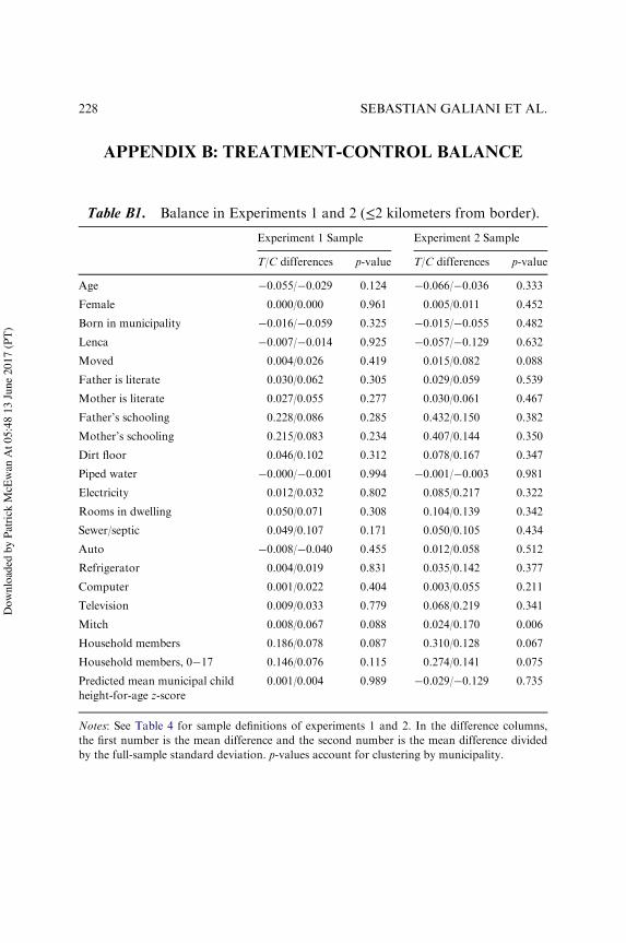
Table B1. Balance in Experiments 1 and 2 (≤2 kilometers from border).

Experiment 1 Sample Experiment 2 Sample

T/C differences p-value T/C differences p-value

Age !0.055/!0.029 0.124 !0.066/!0.036 0.333

Female 0.000/0.000 0.961 0.005/0.011 0.452

Born in municipality !0.016/!0.059 0.325 !0.015/!0.055 0.482

Lenca !0.007/!0.014 0.925 !0.057/!0.129 0.632

Moved 0.004/0.026 0.419 0.015/0.082 0.088

Father is literate 0.030/0.062 0.305 0.029/0.059 0.539

Mother is literate 0.027/0.055 0.277 0.030/0.061 0.467

Father’s schooling 0.228/0.086 0.285 0.432/0.150 0.382

Mother’s schooling 0.215/0.083 0.234 0.407/0.144 0.350

Dirt floor 0.046/0.102 0.312 0.078/0.167 0.347

Piped water !0.000/!0.001 0.994 !0.001/!0.003 0.981

Electricity 0.012/0.032 0.802 0.085/0.217 0.322

Rooms in dwelling 0.050/0.071 0.308 0.104/0.139 0.342

Sewer/septic 0.049/0.107 0.171 0.050/0.105 0.434

Auto !0.008/!0.040 0.455 0.012/0.058 0.512

Refrigerator 0.004/0.019 0.831 0.035/0.142 0.377

Computer 0.001/0.022 0.404 0.003/0.055 0.211

Television 0.009/0.033 0.779 0.068/0.219 0.341

Mitch 0.008/0.067 0.088 0.024/0.170 0.006

Household members 0.186/0.078 0.087 0.310/0.128 0.067

Household members, 0!17 0.146/0.076 0.115 0.274/0.141 0.075

Predicted mean municipal childheight-for-age z-score

0.001/0.004 0.989 !0.029/!0.129 0.735

Notes: See Table 4 for sample definitions of experiments 1 and 2. In the difference columns,the first number is the mean difference and the second number is the mean difference dividedby the full-sample standard deviation. p-values account for clustering by municipality.

228 SEBASTIAN GALIANI ET AL.

Dow

nloa

ded

by P

atric

k M

cEw

an A

t 05:

48 1

3 Ju

ne 2

017

(PT)

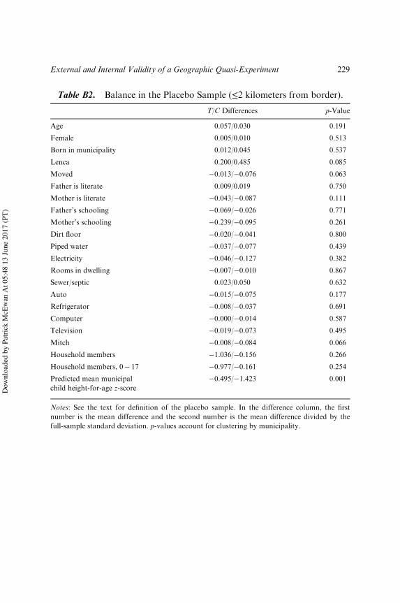
Table B2. Balance in the Placebo Sample (≤2 kilometers from border).

T/C Differences p-Value

Age 0.057/0.030 0.191

Female 0.005/0.010 0.513

Born in municipality 0.012/0.045 0.537

Lenca 0.200/0.485 0.085

Moved !0.013/!0.076 0.063

Father is literate 0.009/0.019 0.750

Mother is literate !0.043/!0.087 0.111

Father’s schooling !0.069/!0.026 0.771

Mother’s schooling !0.239/!0.095 0.261

Dirt floor !0.020/!0.041 0.800

Piped water !0.037/!0.077 0.439

Electricity !0.046/!0.127 0.382

Rooms in dwelling !0.007/!0.010 0.867

Sewer/septic 0.023/0.050 0.632

Auto !0.015/!0.075 0.177

Refrigerator !0.008/!0.037 0.691

Computer !0.000/!0.014 0.587

Television !0.019/!0.073 0.495

Mitch !0.008/!0.084 0.066

Household members !1.036/!0.156 0.266

Household members, 0! 17 !0.977/!0.161 0.254

Predicted mean municipalchild height-for-age z-score

!0.495/!1.423 0.001

Notes: See the text for definition of the placebo sample. In the difference column, the firstnumber is the mean difference and the second number is the mean difference divided by thefull-sample standard deviation. p-values account for clustering by municipality.

229External and Internal Validity of a Geographic Quasi-Experiment

Dow

nloa

ded

by P

atric

k M

cEw

an A

t 05:

48 1

3 Ju

ne 2

017

(PT)

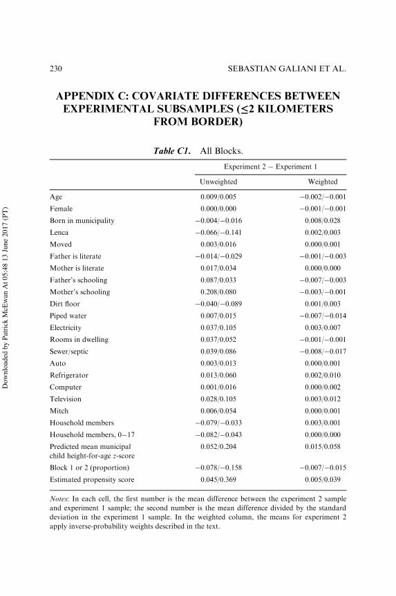
APPENDIX C: COVARIATE DIFFERENCES BETWEENEXPERIMENTAL SUBSAMPLES (≤2 KILOMETERS

FROM BORDER)

Table C1. All Blocks.

Experiment 2 ! Experiment 1

Unweighted Weighted

Age 0.009/0.005 !0.002/!0.001

Female 0.000/0.000 !0.001/!0.001

Born in municipality !0.004/!0.016 0.008/0.028

Lenca !0.066/!0.141 0.002/0.003

Moved 0.003/0.016 0.000/0.001

Father is literate !0.014/!0.029 !0.001/!0.003

Mother is literate 0.017/0.034 0.000/0.000

Father’s schooling 0.087/0.033 !0.007/!0.003

Mother’s schooling 0.208/0.080 !0.003/!0.001

Dirt floor !0.040/!0.089 0.001/0.003

Piped water 0.007/0.015 !0.007/!0.014

Electricity 0.037/0.105 0.003/0.007

Rooms in dwelling 0.037/0.052 !0.001/!0.001

Sewer/septic 0.039/0.086 !0.008/!0.017

Auto 0.003/0.013 0.000/0.001

Refrigerator 0.013/0.060 0.002/0.010

Computer 0.001/0.016 0.000/0.002

Television 0.028/0.105 0.003/0.012

Mitch 0.006/0.054 0.000/0.001

Household members !0.079/!0.033 0.003/0.001

Household members, 0!17 !0.082/!0.043 0.000/0.000

Predicted mean municipalchild height-for-age z-score

0.052/0.204 0.015/0.058

Block 1 or 2 (proportion) !0.078/!0.158 !0.007/!0.015

Estimated propensity score 0.045/0.369 0.005/0.039

Notes: In each cell, the first number is the mean difference between the experiment 2 sampleand experiment 1 sample; the second number is the mean difference divided by the standarddeviation in the experiment 1 sample. In the weighted column, the means for experiment 2apply inverse-probability weights described in the text.

230 SEBASTIAN GALIANI ET AL.

Dow

nloa

ded

by P

atric

k M

cEw

an A

t 05:

48 1

3 Ju

ne 2

017

(PT)

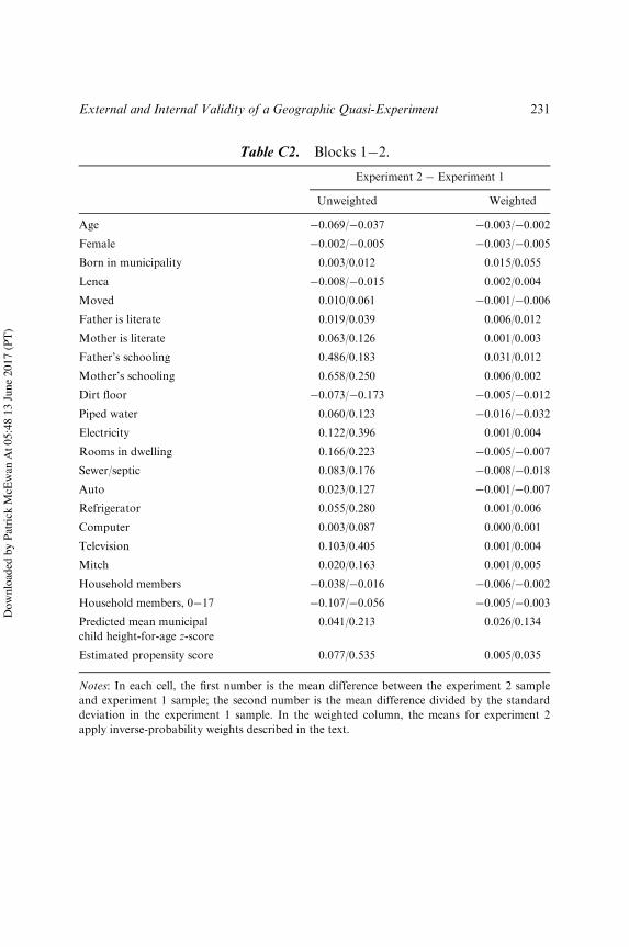
Table C2. Blocks 1!2.

Experiment 2 ! Experiment 1

Unweighted Weighted

Age !0.069/!0.037 !0.003/!0.002

Female !0.002/!0.005 !0.003/!0.005

Born in municipality 0.003/0.012 0.015/0.055

Lenca !0.008/!0.015 0.002/0.004

Moved 0.010/0.061 !0.001/!0.006

Father is literate 0.019/0.039 0.006/0.012

Mother is literate 0.063/0.126 0.001/0.003

Father’s schooling 0.486/0.183 0.031/0.012

Mother’s schooling 0.658/0.250 0.006/0.002

Dirt floor !0.073/!0.173 !0.005/!0.012

Piped water 0.060/0.123 !0.016/!0.032

Electricity 0.122/0.396 0.001/0.004

Rooms in dwelling 0.166/0.223 !0.005/!0.007

Sewer/septic 0.083/0.176 !0.008/!0.018

Auto 0.023/0.127 !0.001/!0.007

Refrigerator 0.055/0.280 0.001/0.006

Computer 0.003/0.087 0.000/0.001

Television 0.103/0.405 0.001/0.004

Mitch 0.020/0.163 0.001/0.005

Household members !0.038/!0.016 !0.006/!0.002

Household members, 0!17 !0.107/!0.056 !0.005/!0.003

Predicted mean municipalchild height-for-age z-score

0.041/0.213 0.026/0.134

Estimated propensity score 0.077/0.535 0.005/0.035

Notes: In each cell, the first number is the mean difference between the experiment 2 sampleand experiment 1 sample; the second number is the mean difference divided by the standarddeviation in the experiment 1 sample. In the weighted column, the means for experiment 2apply inverse-probability weights described in the text.

231External and Internal Validity of a Geographic Quasi-Experiment

Dow

nloa

ded

by P

atric

k M

cEw

an A

t 05:

48 1

3 Ju

ne 2

017

(PT)

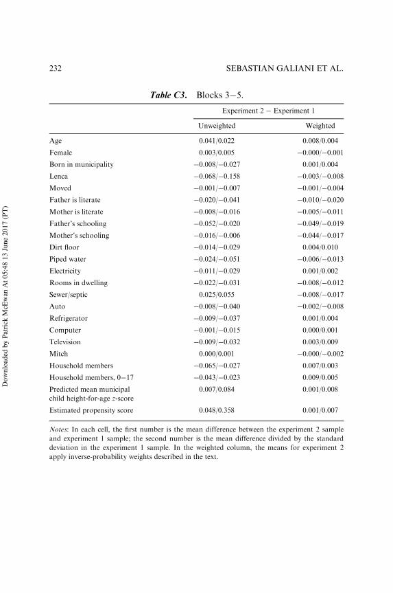
Table C3. Blocks 3!5.

Experiment 2 ! Experiment 1

Unweighted Weighted

Age 0.041/0.022 0.008/0.004

Female 0.003/0.005 !0.000/!0.001

Born in municipality !0.008/!0.027 0.001/0.004

Lenca !0.068/!0.158 !0.003/!0.008

Moved !0.001/!0.007 !0.001/!0.004

Father is literate !0.020/!0.041 !0.010/!0.020

Mother is literate !0.008/!0.016 !0.005/!0.011

Father’s schooling !0.052/!0.020 !0.049/!0.019

Mother’s schooling !0.016/!0.006 !0.044/!0.017

Dirt floor !0.014/!0.029 0.004/0.010

Piped water !0.024/!0.051 !0.006/!0.013

Electricity !0.011/!0.029 0.001/0.002

Rooms in dwelling !0.022/!0.031 !0.008/!0.012

Sewer/septic 0.025/0.055 !0.008/!0.017

Auto !0.008/!0.040 !0.002/!0.008

Refrigerator !0.009/!0.037 0.001/0.004

Computer !0.001/!0.015 0.000/0.001

Television !0.009/!0.032 0.003/0.009

Mitch 0.000/0.001 !0.000/!0.002

Household members !0.065/!0.027 0.007/0.003

Household members, 0!17 !0.043/!0.023 0.009/0.005

Predicted mean municipalchild height-for-age z-score

0.007/0.084 0.001/0.008

Estimated propensity score 0.048/0.358 0.001/0.007

Notes: In each cell, the first number is the mean difference between the experiment 2 sampleand experiment 1 sample; the second number is the mean difference divided by the standarddeviation in the experiment 1 sample. In the weighted column, the means for experiment 2apply inverse-probability weights described in the text.

232 SEBASTIAN GALIANI ET AL.

Dow

nloa

ded

by P

atric

k M

cEw

an A

t 05:

48 1

3 Ju

ne 2

017

(PT)

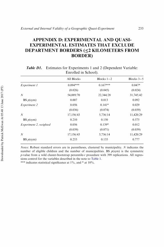
APPENDIX D: EXPERIMENTAL AND QUASI-EXPERIMENTAL ESTIMATES THAT EXCLUDE

DEPARTMENT BORDERS (≤2 KILOMETERS FROMBORDER)

Table D1. Estimates for Experiments 1 and 2 (Dependent Variable:Enrolled in School).

All Blocks Blocks 1!2 Blocks 3!5

Experiment 1 0.094*** 0.167*** 0.047*

(0.026) (0.045) (0.024)

N 54,089/70 22,344/28 31,745/42

BS p(sym) 0.007 0.013 0.092

Experiment 2 0.056 0.141* 0.029

(0.036) (0.074) (0.039)

N 17,156/43 5,736/14 11,420/29

BS p(sym) 0.210 0.150 0.575

Experiment 2, weighted 0.056 0.139* 0.012

(0.039) (0.071) (0.039)

N 17,156/43 5,736/14 11,420/29

BS p(sym) 0.253 0.135 0.777

Notes: Robust standard errors are in parentheses, clustered by municipality. N indicates thenumber of eligible children and the number of municipalities. BS p(sym) is the symmetricp-value from a wild cluster-bootstrap percentile-t procedure with 399 replications. All regres-sions control for the variables described in the note to Table 1.*** indicates statistical significance at 1%, and * at 10%.

233External and Internal Validity of a Geographic Quasi-Experiment

Dow

nloa

ded

by P

atric

k M

cEw

an A

t 05:

48 1

3 Ju

ne 2

017

(PT)

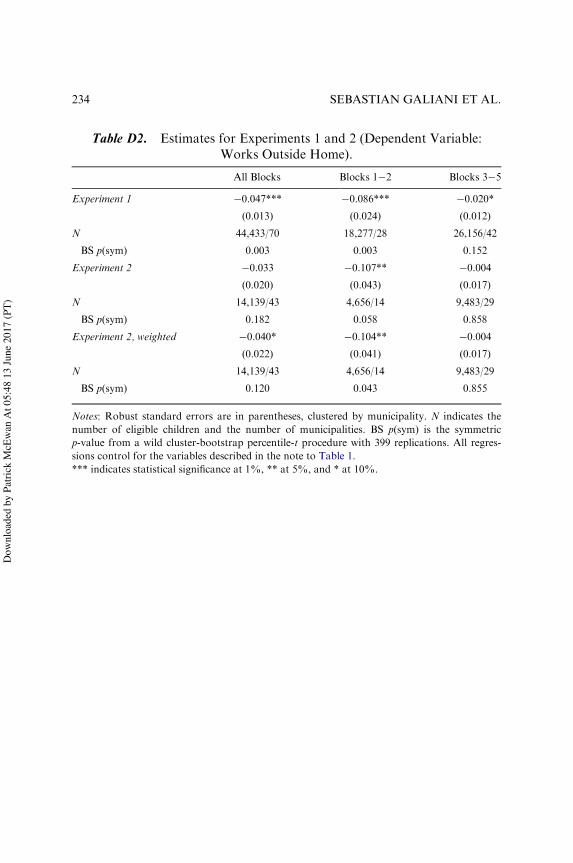
Table D2. Estimates for Experiments 1 and 2 (Dependent Variable:Works Outside Home).

All Blocks Blocks 1!2 Blocks 3!5

Experiment 1 !0.047*** !0.086*** !0.020*

(0.013) (0.024) (0.012)

N 44,433/70 18,277/28 26,156/42

BS p(sym) 0.003 0.003 0.152

Experiment 2 !0.033 !0.107** !0.004

(0.020) (0.043) (0.017)

N 14,139/43 4,656/14 9,483/29

BS p(sym) 0.182 0.058 0.858

Experiment 2, weighted !0.040* !0.104** !0.004

(0.022) (0.041) (0.017)

N 14,139/43 4,656/14 9,483/29

BS p(sym) 0.120 0.043 0.855

Notes: Robust standard errors are in parentheses, clustered by municipality. N indicates thenumber of eligible children and the number of municipalities. BS p(sym) is the symmetricp-value from a wild cluster-bootstrap percentile-t procedure with 399 replications. All regres-sions control for the variables described in the note to Table 1.*** indicates statistical significance at 1%, ** at 5%, and * at 10%.

234 SEBASTIAN GALIANI ET AL.

Dow

nloa

ded

by P

atric

k M

cEw

an A

t 05:

48 1

3 Ju

ne 2

017

(PT)

Table D3. Estimates for Experiments 1 and 2 (Dependent Variable:Works Only in Home).

All Blocks Blocks 1!2 Blocks 3!5

Experiment 1 !0.042*** !0.061** !0.029*

(0.014) (0.024) (0.015)

N 44,433/70 18,277/28 26,156/42

BS p(sym) 0.018 0.075 0.105

Experiment 2 !0.016 !0.023 !0.015

(0.020) (0.030) (0.024)

N 14,139/43 4,656/14 9,483/29

BS p(sym) 0.545 0.502 0.578

Experiment 2, weighted !0.008 !0.022 !0.001

(0.020) (0.030) (0.024)

N 14,139/43 4,656/14 9,483/29

BS p(sym) 0.790 0.545 0.958

Notes: Robust standard errors are in parentheses, clustered by municipality. N indicates thenumber of eligible children and the number of municipalities. BS p(sym) is the symmetricp-value from a wild cluster-bootstrap percentile-t procedure with 399 replications. All regres-sions control for the variables described in the note to Table 1.*** indicates statistical significance at 1%, ** at 5%, and * at 10%.

235External and Internal Validity of a Geographic Quasi-Experiment

Dow

nloa

ded

by P

atric

k M

cEw

an A

t 05:

48 1

3 Ju

ne 2

017

(PT)

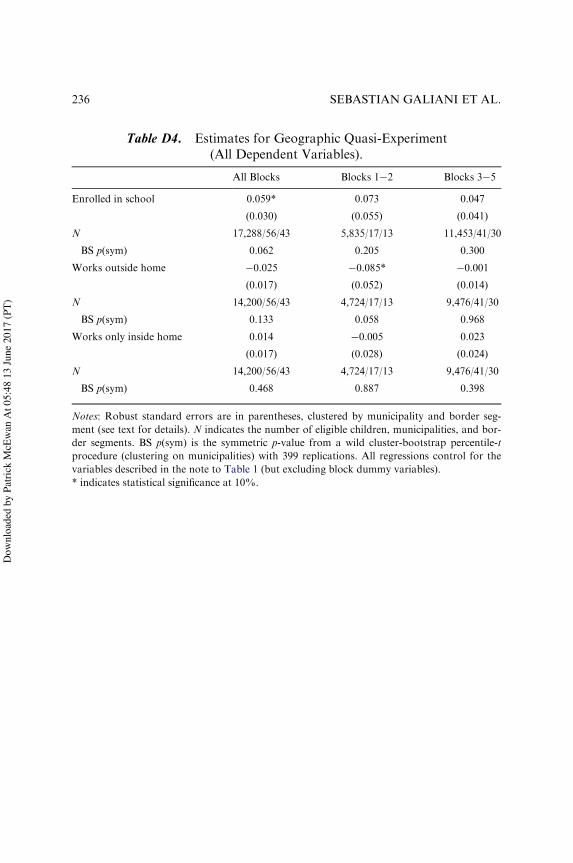
Table D4. Estimates for Geographic Quasi-Experiment(All Dependent Variables).

All Blocks Blocks 1!2 Blocks 3!5

Enrolled in school 0.059* 0.073 0.047

(0.030) (0.055) (0.041)

N 17,288/56/43 5,835/17/13 11,453/41/30

BS p(sym) 0.062 0.205 0.300

Works outside home !0.025 !0.085* !0.001

(0.017) (0.052) (0.014)

N 14,200/56/43 4,724/17/13 9,476/41/30

BS p(sym) 0.133 0.058 0.968

Works only inside home 0.014 !0.005 0.023

(0.017) (0.028) (0.024)

N 14,200/56/43 4,724/17/13 9,476/41/30

BS p(sym) 0.468 0.887 0.398

Notes: Robust standard errors are in parentheses, clustered by municipality and border seg-ment (see text for details). N indicates the number of eligible children, municipalities, and bor-der segments. BS p(sym) is the symmetric p-value from a wild cluster-bootstrap percentile-tprocedure (clustering on municipalities) with 399 replications. All regressions control for thevariables described in the note to Table 1 (but excluding block dummy variables).* indicates statistical significance at 10%.

236 SEBASTIAN GALIANI ET AL.

Dow

nloa

ded

by P

atric

k M

cEw

an A

t 05:

48 1

3 Ju

ne 2

017

(PT)