Embed Size (px)
Citation preview
MIT Center for Transportation & Logistics
CTL.SC1x -Supply Chain & Logistics Fundamentals
Extensions to EOQ Model
CTL.SC1x - Supply Chain and Logistics Fundamentals Lesson: Extensions to EOQ Model
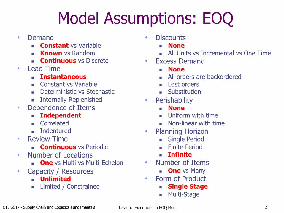
Model Assumptions: EOQ • Demand
n Constant vs Variable n Known vs Random n Continuous vs Discrete
• Lead Time n Instantaneous n Constant vs Variable n Deterministic vs Stochastic n Internally Replenished
• Dependence of Items n Independent n Correlated n Indentured
• Review Time n Continuous vs Periodic
• Number of Locations n One vs Multi vs Multi-Echelon
• Capacity / Resources n Unlimited n Limited / Constrained
• Discounts n None n All Units vs Incremental vs One Time
• Excess Demand n None n All orders are backordered n Lost orders n Substitution
• Perishability n None n Uniform with time n Non-linear with time
• Planning Horizon n Single Period n Finite Period n Infinite
• Number of Items n One vs Many
• Form of Product n Single Stage n Multi-Stage
2
CTL.SC1x - Supply Chain and Logistics Fundamentals Lesson: Extensions to EOQ Model
Non-Instantaneous Leadtime
3
CTL.SC1x - Supply Chain and Logistics Fundamentals Lesson: Extensions to EOQ Model
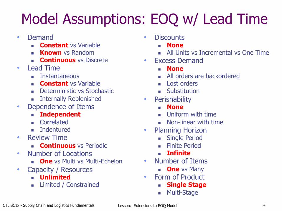
Model Assumptions: EOQ w/ Lead Time • Demand
n Constant vs Variable n Known vs Random n Continuous vs Discrete
• Lead Time n Instantaneous n Constant vs Variable n Deterministic vs Stochastic n Internally Replenished
• Dependence of Items n Independent n Correlated n Indentured
• Review Time n Continuous vs Periodic
• Number of Locations n One vs Multi vs Multi-Echelon
• Capacity / Resources n Unlimited n Limited / Constrained
• Discounts n None n All Units vs Incremental vs One Time
• Excess Demand n None n All orders are backordered n Lost orders n Substitution
• Perishability n None n Uniform with time n Non-linear with time
• Planning Horizon n Single Period n Finite Period n Infinite
• Number of Items n One vs Many
• Form of Product n Single Stage n Multi-Stage
4
CTL.SC1x - Supply Chain and Logistics Fundamentals Lesson: Extensions to EOQ Model
Extensions: Leadtime > 0
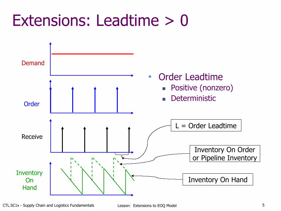
• Order Leadtime n Positive (nonzero) n Deterministic
Inventory On
Hand
Receive
Order
Demand
L = Order Leadtime
Inventory On Order or Pipeline Inventory
Inventory On Hand
5
CTL.SC1x - Supply Chain and Logistics Fundamentals Lesson: Extensions to EOQ Model
Extensions: Leadtime > 0
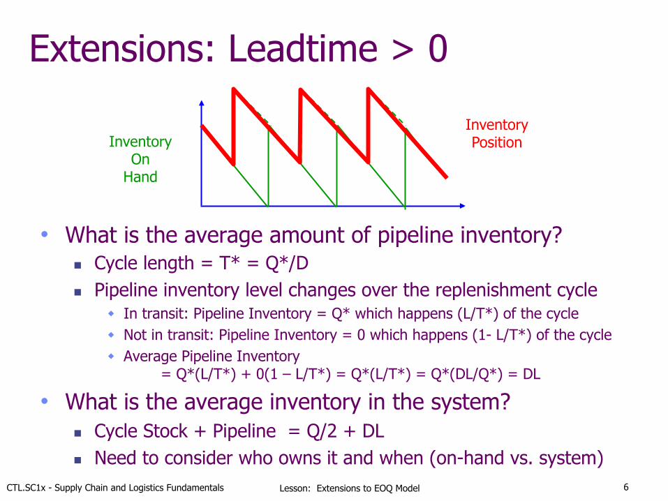
• What is the average amount of pipeline inventory? n Cycle length = T* = Q*/D
n Pipeline inventory level changes over the replenishment cycle w In transit: Pipeline Inventory = Q* which happens (L/T*) of the cycle w Not in transit: Pipeline Inventory = 0 which happens (1- L/T*) of the cycle w Average Pipeline Inventory
= Q*(L/T*) + 0(1 – L/T*) = Q*(L/T*) = Q*(DL/Q*) = DL
• What is the average inventory in the system? n Cycle Stock + Pipeline = Q/2 + DL n Need to consider who owns it and when (on-hand vs. system)
6
Inventory On
Hand
Inventory Position
CTL.SC1x - Supply Chain and Logistics Fundamentals Lesson: Extensions to EOQ Model
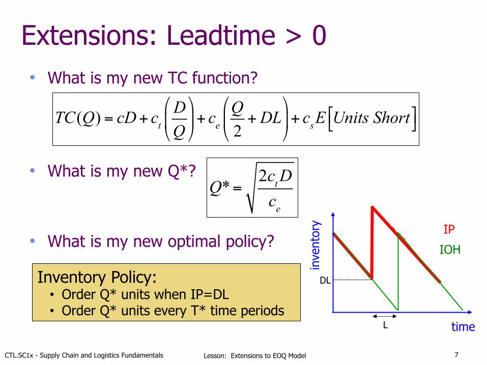
Extensions: Leadtime > 0 • What is my new TC function?
• What is my new Q*?
• What is my new optimal policy?
7
TC(Q) = cD+ ctDQ!
"#
$
%&+ ce
Q2+DL
!
"#
$
%&+ csE Units Short'( )*
Q*= 2ctDce
IP
DL
L
Inventory Policy: • Order Q* units when IP=DL • Order Q* units every T* time periods
IOH
time in
vent
ory

CTL.SC1x - Supply Chain and Logistics Fundamentals Lesson: Extensions to EOQ Model
Quantity Discounts
8
CTL.SC1x - Supply Chain and Logistics Fundamentals Lesson: Extensions to EOQ Model
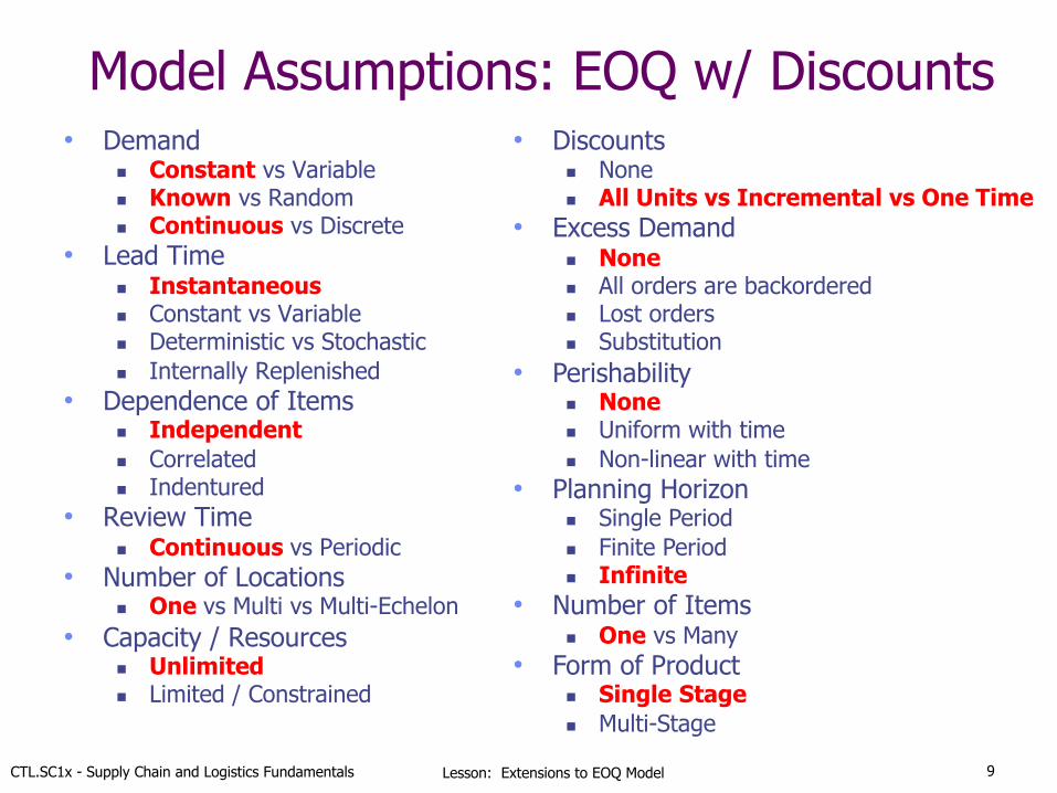
Model Assumptions: EOQ w/ Discounts • Demand
n Constant vs Variable n Known vs Random n Continuous vs Discrete
• Lead Time n Instantaneous n Constant vs Variable n Deterministic vs Stochastic n Internally Replenished
• Dependence of Items n Independent n Correlated n Indentured
• Review Time n Continuous vs Periodic
• Number of Locations n One vs Multi vs Multi-Echelon
• Capacity / Resources n Unlimited n Limited / Constrained
• Discounts n None n All Units vs Incremental vs One Time
• Excess Demand n None n All orders are backordered n Lost orders n Substitution
• Perishability n None n Uniform with time n Non-linear with time
• Planning Horizon n Single Period n Finite Period n Infinite
• Number of Items n One vs Many
• Form of Product n Single Stage n Multi-Stage
9
CTL.SC1x - Supply Chain and Logistics Fundamentals Lesson: Extensions to EOQ Model
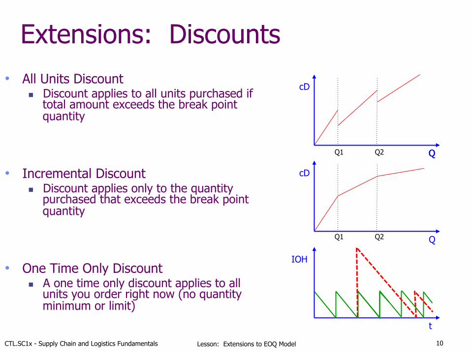
Extensions: Discounts
• All Units Discount n Discount applies to all units purchased if
total amount exceeds the break point quantity
• Incremental Discount n Discount applies only to the quantity
purchased that exceeds the break point quantity
• One Time Only Discount n A one time only discount applies to all
units you order right now (no quantity minimum or limit)
Q Q
cD
Q
cD
t
IOH
Q1 Q2
Q1 Q2
10
CTL.SC1x - Supply Chain and Logistics Fundamentals Lesson: Extensions to EOQ Model
Quantity Discounts: All Units
11
CTL.SC1x - Supply Chain and Logistics Fundamentals Lesson: Extensions to EOQ Model
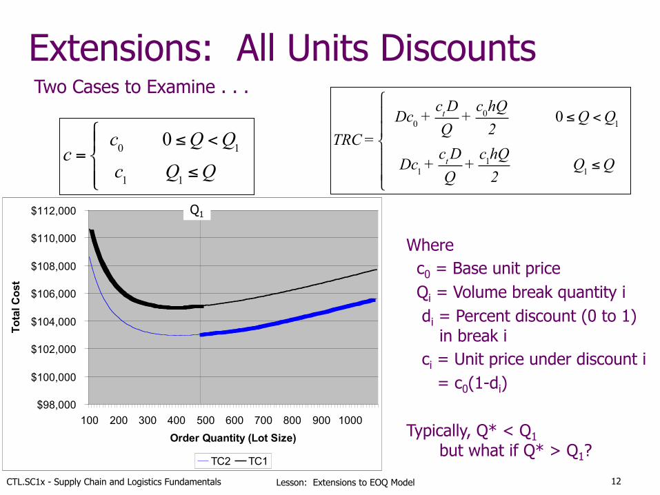
Extensions: All Units Discounts
TRC = Dc0 + ct D
Q + c0hQ
20 ≤Q <Q1
Dc1 + ct DQ
+ c1hQ2
Q1 ≤Q
"
#
$$
%
$$
$98,000
$100,000
$102,000
$104,000
$106,000
$108,000
$110,000
$112,000
100 200 300 400 500 600 700 800 900 1000Order Quantity (Lot Size)
Tota
l Cos
t
TC2 TC1
Qb
c =c0 0 ≤Q <Q1c1 Q1 ≤Q
"#$
%$
Where c0 = Base unit price Qi = Volume break quantity i di = Percent discount (0 to 1)
in break i ci = Unit price under discount i = c0(1-di) Typically, Q* < Q1
but what if Q* > Q1?
Two Cases to Examine . . .
12
Q1
CTL.SC1x - Supply Chain and Logistics Fundamentals Lesson: Extensions to EOQ Model
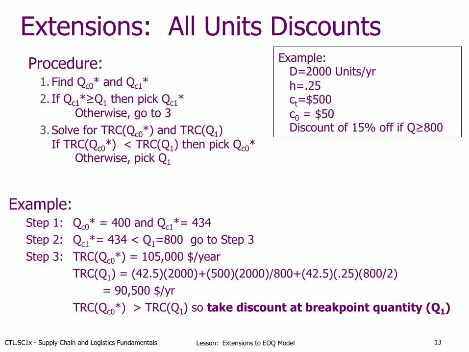
Extensions: All Units Discounts Procedure:
1. Find Qc0* and Qc1* 2. If Qc1*≥Q1 then pick Qc1*
Otherwise, go to 3 3. Solve for TRC(Qc0*) and TRC(Q1)
If TRC(Qc0*) < TRC(Q1) then pick Qc0* Otherwise, pick Q1
Example: D=2000 Units/yr h=.25 ct=$500 c0 = $50 Discount of 15% off if Q≥800
13
Example: Step 1: Qc0* = 400 and Qc1*= 434 Step 2: Qc1*= 434 < Q1=800 go to Step 3 Step 3: TRC(Qc0*) = 105,000 $/year TRC(Q1) = (42.5)(2000)+(500)(2000)/800+(42.5)(.25)(800/2) = 90,500 $/yr TRC(Qc0*) > TRC(Q1) so take discount at breakpoint quantity (Q1)
CTL.SC1x - Supply Chain and Logistics Fundamentals Lesson: Extensions to EOQ Model
Quantity Discounts: Incremental
14

CTL.SC1x - Supply Chain and Logistics Fundamentals Lesson: Extensions to EOQ Model
Extensions: Incremental Discounts • Discount i only applies to quantity purchased above breakpoint i • Trade-off between lower purchase cost and higher carrying costs • Cost of units ordered below breakpoint i are treated as new Fixed Cost (Fi)
Units
Tota
l Pu
rcha
se
Cost
c0 c1 c2
Q1 Q2 (c0-c1)Q1
c1Q1
c0Q1
15
F0 = 0
Fi = Fi−1 + ci−1 − ci( )Qi
Q*i =2D ct + Fi( )
hci
CTL.SC1x - Supply Chain and Logistics Fundamentals Lesson: Extensions to EOQ Model
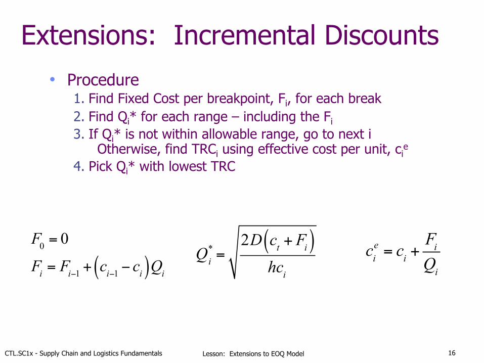
Extensions: Incremental Discounts
• Procedure 1. Find Fixed Cost per breakpoint, Fi, for each break 2. Find Qi* for each range – including the Fi 3. If Qi* is not within allowable range, go to next i
Otherwise, find TRCi using effective cost per unit, cie
4. Pick Qi* with lowest TRC
cie = ci +
FiQi
Q*i =2D ct + Fi( )
hci
16
F0 = 0
Fi = Fi−1 + ci−1 − ci( )Qi

CTL.SC1x - Supply Chain and Logistics Fundamentals Lesson: Extensions to EOQ Model
Quantity Discounts: One Time Buy
17

CTL.SC1x - Supply Chain and Logistics Fundamentals Lesson: Extensions to EOQ Model
Extensions: One Time Discount Suppose you are offered a One Time deal! Should you take it? cg = One time good deal purchase price ($/unit) Qg = One time good deal order quantity (units) TCsp=TC over time covered by special purchase ($)
18
t
IOH

CTL.SC1x - Supply Chain and Logistics Fundamentals Lesson: Extensions to EOQ Model
Extensions: One Time Discount • Compare Options: Normal Price (c) vs. Special Price (cg)
n Find TC for normal price
TC = (CycleTime)(TC* + PurchaseCost)
TC =QgD
!
"##
$
%&& 2cthcD +
QgD
!
"##
$
%&&cD
Savings =TC −TCSP
=QgD
"
#$$
%
&'' 2cthcD +
QgD
"
#$$
%
&''cD
"
#$$
%
&''− cgQg + hcg
Qg2
"
#$$
%
&''QgD
"
#$$
%
&''+ ct
"
#$$
%
&''
n Find the Savings (TC-TCSP)
19
CTL.SC1x - Supply Chain and Logistics Fundamentals Lesson: Extensions to EOQ Model
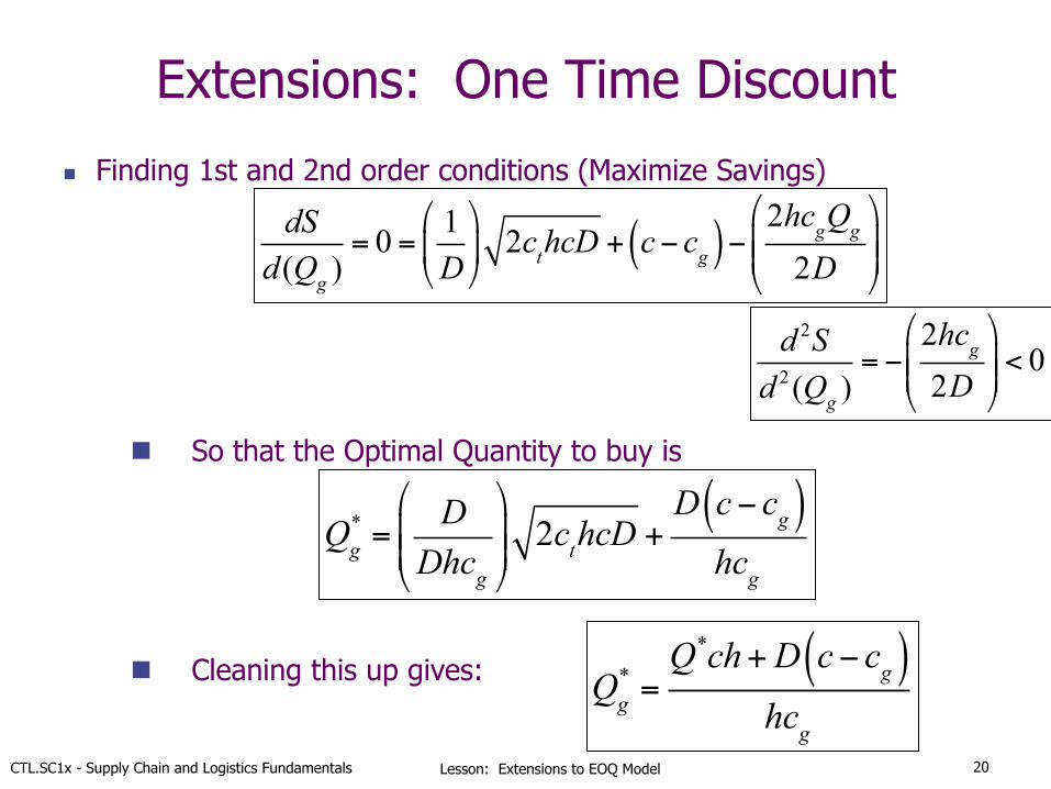
Extensions: One Time Discount
n Finding 1st and 2nd order conditions (Maximize Savings)
d 2Sd 2 (Qg )
= −2hcg2D
!
"##
$
%&&< 0
dSd(Qg )
= 0 = 1D!
"#
$
%& 2cthcD + c− cg( )−
2hcgQg2D
!
"##
$
%&&
Qg* =
DDhcg
!
"##
$
%&& 2cthcD +
D c− cg( )hcg
Qg* =Q*ch+D c− cg( )
hcg
n So that the Optimal Quantity to buy is
n Cleaning this up gives:
20
CTL.SC1x - Supply Chain and Logistics Fundamentals Lesson: Extensions to EOQ Model
Finite Replenishment Economic Production Quantity (EPQ)
21
CTL.SC1x - Supply Chain and Logistics Fundamentals Lesson: Extensions to EOQ Model
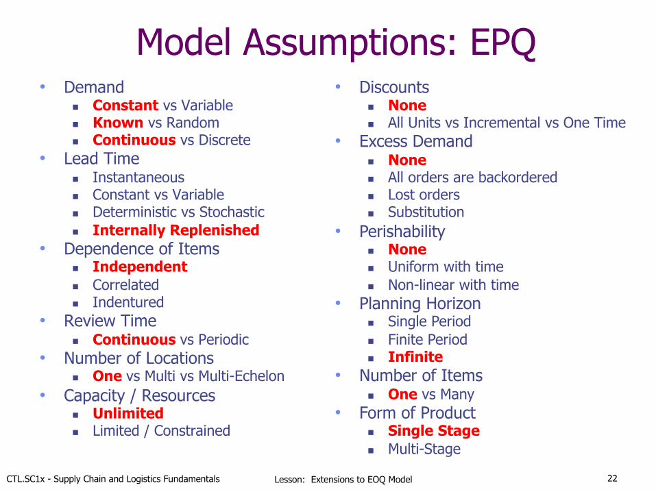
Model Assumptions: EPQ • Demand
n Constant vs Variable n Known vs Random n Continuous vs Discrete
• Lead Time n Instantaneous n Constant vs Variable n Deterministic vs Stochastic n Internally Replenished
• Dependence of Items n Independent n Correlated n Indentured
• Review Time n Continuous vs Periodic
• Number of Locations n One vs Multi vs Multi-Echelon
• Capacity / Resources n Unlimited n Limited / Constrained
• Discounts n None n All Units vs Incremental vs One Time
• Excess Demand n None n All orders are backordered n Lost orders n Substitution
• Perishability n None n Uniform with time n Non-linear with time
• Planning Horizon n Single Period n Finite Period n Infinite
• Number of Items n One vs Many
• Form of Product n Single Stage n Multi-Stage
22
CTL.SC1x - Supply Chain and Logistics Fundamentals Lesson: Extensions to EOQ Model
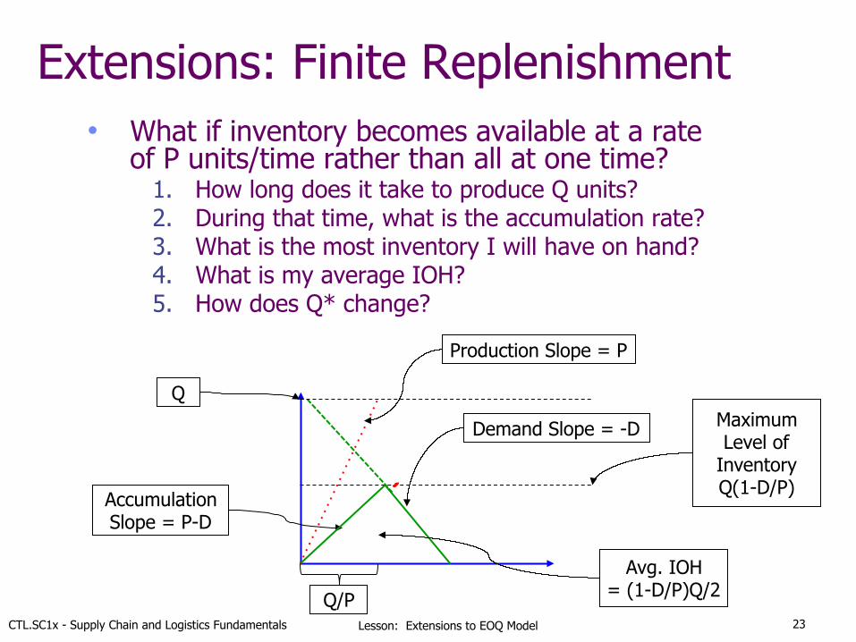
Extensions: Finite Replenishment • What if inventory becomes available at a rate
of P units/time rather than all at one time? 1. How long does it take to produce Q units? 2. During that time, what is the accumulation rate? 3. What is the most inventory I will have on hand? 4. What is my average IOH? 5. How does Q* change?
Maximum Level of
Inventory Q(1-D/P)
Accumulation Slope = P-D
Q/P
Demand Slope = -D
Q
23
Production Slope = P
Avg. IOH = (1-D/P)Q/2
CTL.SC1x - Supply Chain and Logistics Fundamentals Lesson: Extensions to EOQ Model
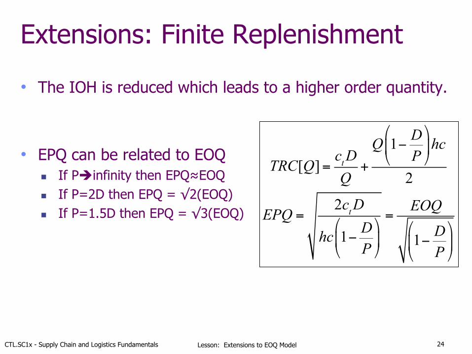
Extensions: Finite Replenishment
TRC[Q]= ctDQ
+
Q 1− DP
"
#$
%
&'hc
2
EPQ = 2ctD
hc 1− DP
"
#$
%
&'
=EOQ
1− DP
"
#$
%
&'
• The IOH is reduced which leads to a higher order quantity.
• EPQ can be related to EOQ n If Pèinfinity then EPQ≈EOQ n If P=2D then EPQ = √2(EOQ) n If P=1.5D then EPQ = √3(EOQ)
24

CTL.SC1x - Supply Chain and Logistics Fundamentals Lesson: Extensions to EOQ Model
Key Points from Lesson
25
CTL.SC1x - Supply Chain and Logistics Fundamentals Lesson: Extensions to EOQ Model
Key Points
• EOQ is a good place to start for most analysis and can be extended to cover many variations: n Non-zero lead times
w No effect on Q* w Monitor Inventory Position vs Inventory on Hand w Changes timing of replenishment (IP≤DL)
n Discounts (All Units, Incremental, One Time Buy) w Common in practice (economies of scale) w Purchase price (c) becomes relevant w Need to estimate costs at breakpoints & compare
n Finite replenishment systems w Items become available incrementally over time w Lowers holding costs and leads to higher EPQ
26
MIT Center for Transportation & Logistics
CTL.SC1x -Supply Chain & Logistics Fundamentals
Questions, Comments, Suggestions? Use the Discussion!