1

Extensions of the Ricardian model

Actual trade is characterized by the exchange of a large number of goods (more than 2!). For example, the

SITC nomenclature has 3118 5-digit product categories. However, the number of goods actually traded is

larger. Some commodities like textiles are well represented (200 entries) but trade classification does not

fully account for the degree of product differentiation of many other items (such as bolt, cars, etc.).

Many goods DFS77 model

Now we want to extend the Ricardian model to the case of many goods using the continuum assumption

originally developed in the paper by Dornbusch, Fisher and Samuelson (1977), published in the American

Economic Review. To simplify the analysis the model assumes a continuous rather than discrete number of

goods. The model allows to study the effects of growth, demand shifts and exogenous technological change.

In each case the focus of the analysis is to determine:

i) the dividing line between exported and imported goods,

ii) the position of the relative wage that assures balanced trade.

2

SUPPLY SIDE

The model assumes that each good is produced with constant unit labor requirement both at home and

abroad. For i-th good, ai represents the unit labor requirement in the home country, while ai* the unit labor

requirement in the foreign country.

Goods can be ranked according to the diminishing home country comparative advantage. Hence, if n goods

are produced we have:

advantageecomparativ

weakest

n

n

i

i

advantageecomparativ

strongest

a

a

a

a

a

a

a

a *...

*...

**

2

2

1

1

Numerical example with 4 goods: A, B, C &D

Assume that unit labor costs are as follows:

ali A B C D

Home (ali) 1 2 3 5

Foreign

(ali*)

12 18 24 30

And relative wages are equal (w/w*): 7.

Home country has a comparative advantage in production of goods: A, B, C and Foreign country in

production of good D

What happens when relative wages are equal 9?

3

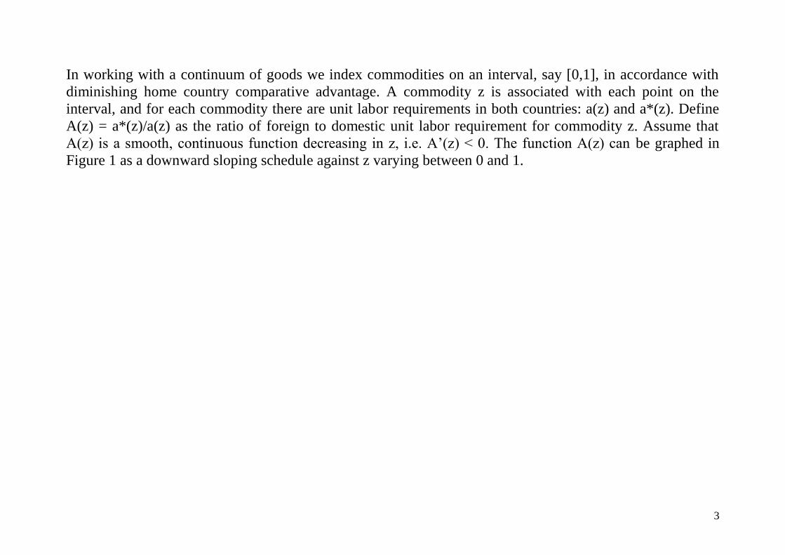
In working with a continuum of goods we index commodities on an interval, say [0,1], in accordance with

diminishing home country comparative advantage. A commodity z is associated with each point on the

interval, and for each commodity there are unit labor requirements in both countries: a(z) and a*(z). Define

A(z) = a*(z)/a(z) as the ratio of foreign to domestic unit labor requirement for commodity z. Assume that

A(z) is a smooth, continuous function decreasing in z, i.e. A’(z) < 0. The function A(z) can be graphed in

Figure 1 as a downward sloping schedule against z varying between 0 and 1.

4

Figure 1. Relative unit requirement function

A(z)

z 1 0

5

Now consider the range of goods produced in the home country (and those produced abroad).

It will be cheaper to produce the good in the home country if unit production cost is smaller than abroad:

a(z)w ≤ a*(z)w*

This is called the efficient specialization condition. If we define relative wage as w/w* = ω, this condition

can be rewritten as:

ω ≤ A(z)

In other words, the good will be produced in the home country if the relative wage is smaller or equal the

relative productivity.

For a given relative wage the home country will produce the range of commodities:

)(~0 zz

while the foreign country will produce the range of commodities:

1)(~ zz

If we know the relative wage ω we can determine the borderline commodity z~ .

6

Figure 2. The pattern of international specialization given the state of technology and relative wages.

A(z)

z 1 0 z

7

DEMAND SIDE

On the demand side we assume homothetic and identical consumer preferences in both countries.

In particular, we assume that the demand functions are derived from a Cobb-Douglas utility function.

In the discrete case we would have:

Y

cpb ii

i

shareeexpenditur

constant

,

where:

n

iib

1

1, and bi = bi*

In the continuous case we have:

Y

zczpzb

)()()( ,

where: 1

0

1)( dzzb , and b(z) = b*(z).

and where:

Y – total income

c(z) – consumption demand for good z

p(z) – price of good z

8

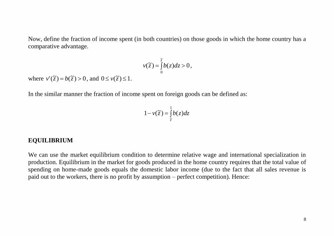
Now, define the fraction of income spent (in both countries) on those goods in which the home country has a

comparative advantage.

z

dzzbzv

~

0

0)()~( ,

where 0)~()~(' zbzv , and .1)~(0 zv

In the similar manner the fraction of income spent on foreign goods can be defined as:

1

~

)()~(1z

dzzbzv

EQUILIBRIUM

We can use the market equilibrium condition to determine relative wage and international specialization in

production. Equilibrium in the market for goods produced in the home country requires that the total value of

spending on home-made goods equals the domestic labor income (due to the fact that all sales revenue is

paid out to the workers, there is no profit by assumption – perfect competition). Hence:

9

)(

goodsouron

eexpenditurworldtotal

goodsmadehome

onspentincomeoffraction

*]*[)~(

incomeour

revenuesales

incomeworldtotal

wLLwwLzv

The above condition associates with each z an value of the relative wage w/w*. The alternative interpretation

of this condition is as follows:

EXPORTSIMPORTS

enditureincomeour

enditureourinimportsofshare

LwzvwLzv

eexpenditurincomeforeign

eexpenditurforeigningoods

madehomeofshare

)(exp

exp

**)~()]~(1[

Hence, the above condition can be interpreted as the balanced trade condition.

10

This condition can be rewritten as:

)*

,~(*

)~(1

)~(

* L

LzB

L

L

zv

zv

w

w

B schedule is upward sloping because an increase in the range of commodities produced at home (at constant

relative wages) lowers our imports and raises our exports. The resulting trade imbalance has to be eliminated

by an increase in our relative wage (that would raise our imports and reduce exports).

The alternative interpretation (home labor market interpretation).

If the number of goods produced at home increases (but wages remain unchanged) then the demand for

home labor would increase (with increasing number of goods produced at home) and the demand for foreign

labor would decrease. In this case the relative wage has to increase to equate the demand for domestic labor

to the existing (fixed) labor supply.

11

Figure 3. The balanced trade condition.

B(z)

z 1 0 z

'z

'

SURPLUS

DEFICIT

12

The final step is to combine the efficient specialization condition and the balanced trade condition.

A(z),

B(Z)

z 1 0 z

13

Effects of increase in relative Foreign country size.

A(z),

B(Z)

z 1 0 z

14

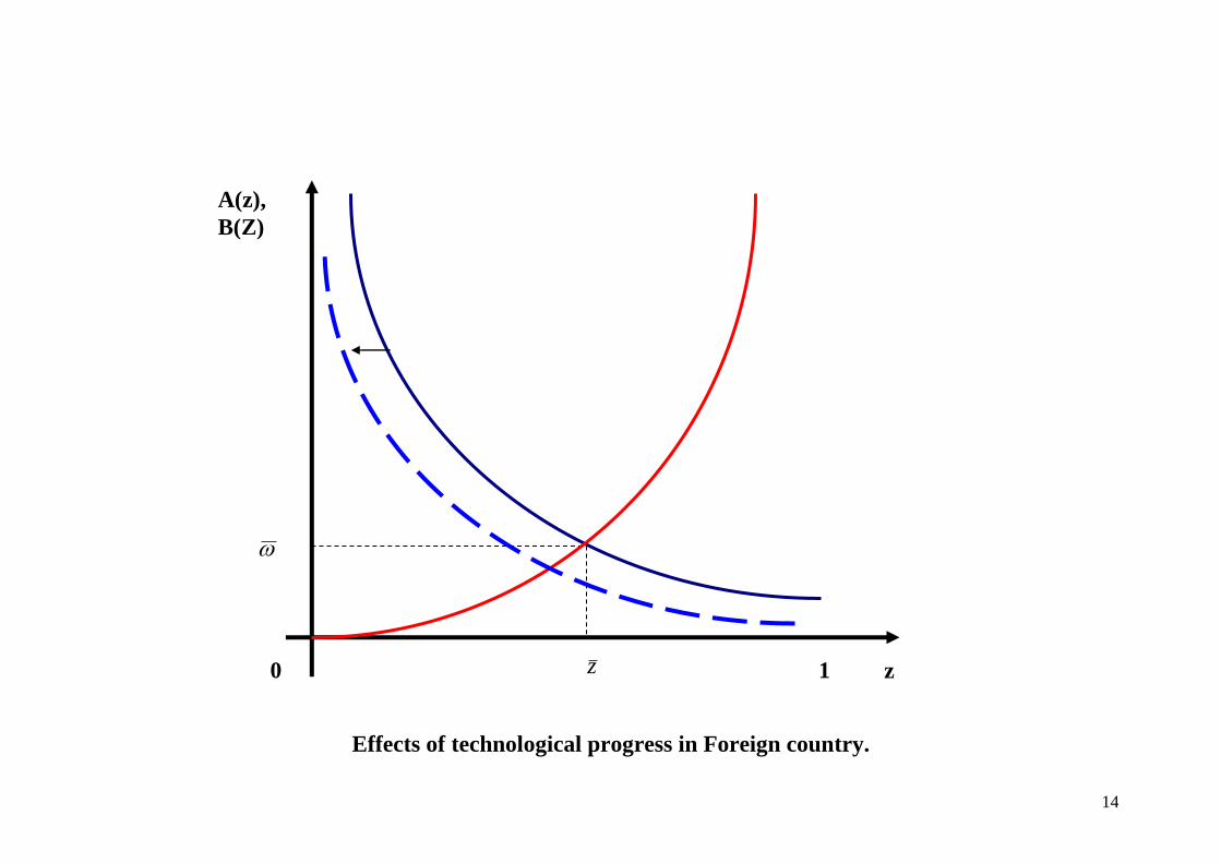
Effects of technological progress in Foreign country.

A(z),

B(Z)

z 1 0 z

15

Empirical tests of Ricardian model

The relationship between trade theory and empirical tests – General remarks

Economists have developed numerous models to explain why international trade takes place. These models

make assumptions that embody STRONG ABSTRACTIONS (such as perfect competition, one factor of

production, etc.) from reality in order to isolate the particular influence of some important variable on the

pattern and the volume of trade. (Empirical research obeys a similar rule, in econometric studies we often

focus on the variable of interest controlling for the impact of other variables).

Otherwise, undertaking an analysis in the real-world environment of imperfect competition, numerous

factors of production, and trade restrictions would be very difficult. These theoretical abstractions allow

economists to investigate the implications of different circumstances for trade flows and economic welfare.

However, some people claim that all these theories are too abstract to be tested empirically.

It is natural for analysts to wonder how well their theoretical predictions correlate with actual empirical data

on international trade. That is why there exists a large body of literature in which economists attempt to test

various aspects of the theory of comparative advantage (or to assess the importance of different explanations

for trade).

BAD NEWS: There is a large number of problems in the empirical work on international trade a trade

analyst must be confronted with.

16

It is very difficult to test theories of comparative advantage directly because they rely on statements

about differences in autarky relative costs and prices across countries. Autarky is virtually an

unobservable situation, and available data would be influenced by international trade. Therefore,

economists often use INDIRECT ways of testing trade theories based on observable variables.

To establish theoretical statements about trade economists make numerous simplifying assumptions

that cannot be true under all realistic circumstances. Even in cases where it is possible to translate

theories into equations that embody observable variables, these equations cannot be expected to hold

literally or without error. Given this constraint, empirical work consists largely of measurement and

judgement rather than precise testing. Therefore you should rather ESTIMATE but DO NOT TEST!

Since trade theories cannot be tested economists must pose a simpler question: “How closely do actual

trade data correspond to the levels predicted by various trade theories?”.

Various international trade theories should not be seen as competing hypotheses. Each theory tends to

focus on a particular aspect of national economies that is expected to induce trade. Each of these

influences operates simultaneously both alone and in conjunction with the others to explain the pattern

and the volume of trade. The task for an economist is to assess the relative importance of various trade

determinants. Therefore, remember that each theory works in its own limited domain for which it was

created.

GOOD NEWS: Despite the aforementioned problems economists made great progress in studying the effects

of various influences on the patterns of international trade. In particular it is worth examining some of the

important work on the determinants of comparative advantage.

17

Early tests of the Ricardian model

The Ricardian model rests on the assumption of different production technologies in different countries

generating varying labor productivities. These labor productivities determine comparative advantage. Tests

of the Ricardian model attempt to find relationships between relative labor productivity and international

trade flows.

The sharpest prediction of the Ricardian model that countries are completely specialized in the goods they

export is rejected in practice. Countries produce also goods they import and a whole range of non-traded

goods. Nevertheless, it is interesting to examine how strongly differences in labor efficiency correlate with

exports. Therefore, looser versions of the Ricardian model are studied (that allow for, for example, across

industry wage variation).

MacDougall (1951) tests

The pioneering empirical work on the Ricardian model was done in the 1950s by G. MacDougall (1951),

published in Economic Journal, who computed simple measures of average labor productivity (output per

worker) in the United States and the United Kingdom for the year 1937.

MacDougall hypothesized that, given that American wage rate was approximately twice that in the UK, US

firms should have an export advantage in manufacturing sectors for which U.S. labor productivity

exceeded twice the level in the UK.

18

He tested this hypothesis by calculating the ratios of US exports to UK exports of 25 products to countries

other than themselves (because at that time trade barriers greatly influenced bilateral trade between the US

and the UK while in other countries exporters from both countries faced largely equivalent market conditions

and could compete on an equal footing).

MacDougall test results were very supportive of the Ricardian model. 20 of 25 products satisfied the simple

prediction that in cases where US productivity exceeded twice the UK level, the ratio of US exports to UK

exports exceeded one (while in other cases the ratio was smaller than unity).

TABLE. US and UK relative unit labor requirements and exports to third countries in 1937

aUK/aUS >2

(US output per worker more than twice the UK output)

US exports / UK exports

Wireless sets and valves 8

Pig iron 5

Motor cars 4

Glass containers 3.5

Tin cans 3

Machinery 1.5

Paper 1

19

1.4 < aUK/aUS < 2

(US output per worker less than twice the UK output)

UK exports / US exports

Cigarettes 2

Linoleum 3

Hosiery 3

Leather footwear 3

Coke 5

Rayon weaving 5

Cotton goods 9

Rayon making 11

Beer 18

aUK/aUS < 1.4

(US output per worker less than 1.4 the UK output)

UK exports / US exports

Cement 11

Men’s/boys’ coats 23

Margarine 32

Woolen and worsted 250

Exceptions: US output per worker more than twice UK output per worker but UK exports exceed US

exports: electric lamps, rubber tyres, soap, biscuits and matches. These represent about 3% of the value of

trade in the commodities listed.

Source: MacDougall (1951, p.698).

20

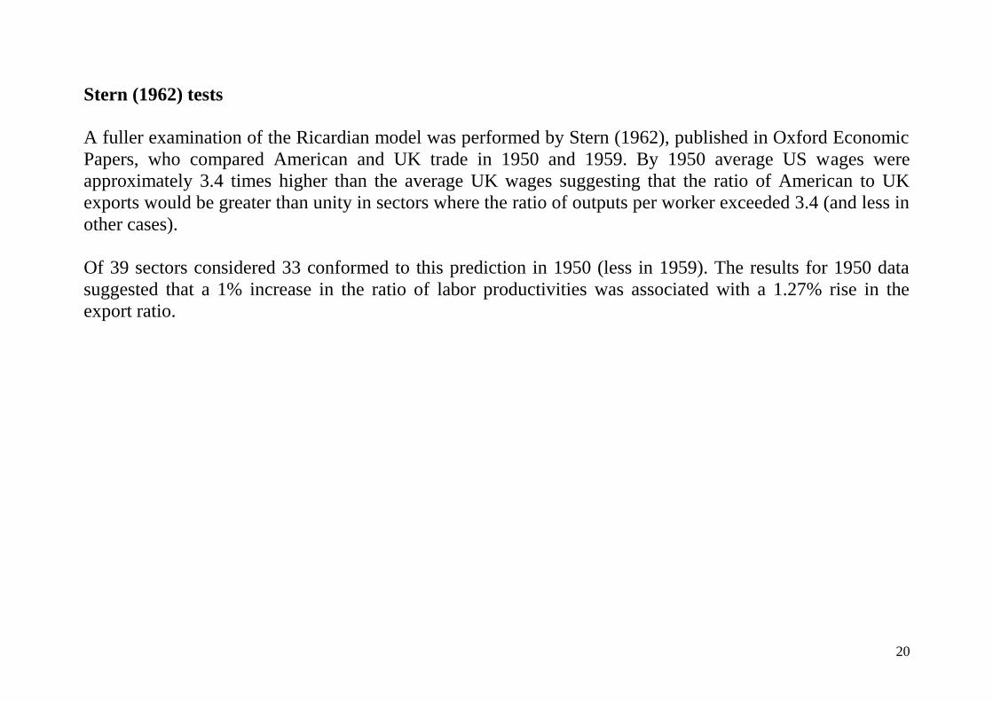
Stern (1962) tests

A fuller examination of the Ricardian model was performed by Stern (1962), published in Oxford Economic

Papers, who compared American and UK trade in 1950 and 1959. By 1950 average US wages were

approximately 3.4 times higher than the average UK wages suggesting that the ratio of American to UK

exports would be greater than unity in sectors where the ratio of outputs per worker exceeded 3.4 (and less in

other cases).

Of 39 sectors considered 33 conformed to this prediction in 1950 (less in 1959). The results for 1950 data

suggested that a 1% increase in the ratio of labor productivities was associated with a 1.27% rise in the

export ratio.

21

PROBLEMS WITH THE EARLY TESTS OF THE RICARDIAN MODEL

The early studies by MacDougall (1951) and Stern (1962) seemed to provide encouraging support for the

Ricardian model. In fact, it is surprising that economists have not devoted much additional effort to such

analysis in order to verify more conclusively that labor productivity differences constitute an important

determinant of international trade.

In interpreting the results of empirical studies we must keep two important caveats in mind:

The empirical specifications used in these studies were exceedingly simple an did not control for the

potential effects of other determinants of trade (such as transport costs, imperfect competition, product

differentiation, etc.).

The results found by MacDougall and Stern are consistent with other trade theories as well. For

example, in a world where trade is caused by differences in factor endowments but where factor prices

are not equalized the relative productivity of labor will tend to be higher in capital-abundant countries

(as more capital intensive production techniques will be used in all industries). Accordingly, the results

may have simply captured the effects on trade of American capital abundance and UK labor abundance

in that period.

22

CONCLUDING REMARKS

The Ricardian model seems to raise more questions about the sources of comparative advantage than it

answers. The model provides no guide as to how labor productivity and comparative advantage can be

expected to evolve since it gives no explanation for differences in labor productivities across countries. This

sets on of the tasks for more complex models such as the Heckscher-Ohlin-Samuelson model with two

factors of production and the factor specific model with three factors of production.