Extended Formulations

in Combinatorial Optimization

Michele Conforti ∗

Universita di Padova, conforti@math.unipd.it

Gerard Cornuejols †

Carnegie Mellon University and Universite d’Aix-Marseillegc0v@andrew.cmu.edu

Giacomo Zambelli ‡

Universita di Padova, giacomo@math.unipd.it

November 2009, revised February 2010

Abstract

This survey is concerned with the size of perfect formulations for combinatorial op-timization problems. By ”perfect formulation”, we mean a system of linear inequalitiesthat describes the convex hull of feasible solutions, viewed as vectors. Natural perfectformulations often have a number of inequalities that is exponential in the size of thedata needed to describe the problem. Here we are particularly interested in situationswhere the addition of a polynomial number of extra variables allows a formulation witha polynomial number of inequalities. Such formulations are called ”compact extendedformulations”. We survey various tools for deriving and studying extended formulations,such as Fourier’s procedure for projection, Minkowski-Weyl’s theorem, Balas’ theoremfor the union of polyhedra, Yannakakis’ theorem on the size of an extended formulation,dynamic programming, and variable discretization. For each tool that we introduce, wepresent one or several examples of how this tool is applied. In particular, we presentcompact extended formulations for several graph problems involving cuts, trees, cyclesand matchings, and for the mixing set. We also present Bienstock’s approximate compactextended formulation for the knapsack problem, Goemans’ result on the size of an ex-tended formulation for the permutahedron, and the Faenza-Kaibel extended formulationfor orbitopes.

∗Supported by the Progetto di Eccellenza 2008-2009 of the Fondazione Cassa di Risparmio di Padova eRovigo

†Supported by NSF grant CMMI0653419, ONR grant N00014-09-1-0133 and ANR grant BLAN06-1-138894.‡Supported by the Progetto di Eccellenza 2008-2009 of the Fondazione Cassa di Risparmio di Padova e

Rovigo

1

1 Introduction

Many combinatorial optimization problems can be written in the following form: Optimizea linear function of a vector x of feasible solutions, where the feasible set is given by linearconstraints (inequalities and/or equalities) and the restriction that some (or all) componentsof the vector x are integral. A ”perfect” formulation is one where the linear constraints de-scribe the convex hull of feasible solutions. The interest in perfect formulations comes fromthe fact that the corresponding combinatorial optimization problems can then be solved aslinear programs. The number of linear constraints needed in a perfect formulation is oftenexponential in the size of the data used to describe the problem. In this survey, we studysituations where the addition of a polynomial number of new variables allows a formulationwith polynomially many linear constraints. When this is possible, we say that the problemhas a ”compact extended formulation”. Such formulations are important in integer pro-gramming and combinatorial optimization, both theory and computations. In this paper, wesurvey various tools for deriving and studying extended formulations. For each tool that weintroduce, we present one or several examples of how this tool is applied.

Projection is the most basic tool for relating extended formulations to formulations in theoriginal space of variables. There are two classical methods for projecting, one uses the notionof projection cone and the other is Fourier’s procedure. We show how Fourier’s method canbe used to derive Barahona’s compact extended formulation of the cycle relaxation of the cutpolytope. The projection cone idea is used to derive the Balas-Pulleyblank formulation ofthe perfectly matchable subgraphs of a graph. It can also be used for other graph problems(st-cut dominant, arborescences, trees, cuts, cycle cone).

We present Minkowski-Weyl’s theorem and apply it to derive a compact extended formu-lation for the mixing set.

Balas’ theorem for the union of polyhedra is another very useful tool. We apply it to sev-eral problems: All even subsets, cut dominant, an approximate compact extended formulationfor the knapsack problem, and the continuous mixing set.

A striking theorem of Yannakakis gives a lower bound on the size of an extended for-mulation for a polytope. We extend this result to polyhedra and we apply it to extendedformulations for spanning trees, matchings, stable sets, and the permutahedron.

The next tool that we present is dynamic programming. We show how it implies extendedformulations for the knapsack problem, stable sets in distance claw-free graphs, and packingand partitioning orbitopes.

Finally, we discuss variable discretization, a new tool that has proved extremely usefulwhen dealing with mixed integer linear sets. This approach has been particularly successfulin dealing with problems arising in lot-sizing.

We now give a formal presentation of the results. Given a set S ⊂ Rn and a linearsubspace L of Rn, the orthogonal projection of S onto L is the set of all points u ∈ L suchthat there exists a vector v ∈ Rn orthogonal to L such that u + v ∈ S.

We are interested in orthogonal projections onto the space L = x ∈ Rn : xi = 0, i ∈N \M where N = 1, . . . , n and M is a subset of N . We denote the set x ∈ RM : ∃z ∈RN\M s.t.

(xz

)∈ S by projx(S).

2

Our interest comes from the fact that the two programs

maxf(x) : x ∈ projx(S) and maxf(x) + 0z :(

xz

)∈ S

are equivalent. However, sometimes the set S is easier to describe than its projection, solooking at the second problem is easier. In this survey, we study sets of the type:

X = x ∈ RN : A′x ≤ b′, xi integer, i ∈ I ⊆ N (1)

that arise in combinatorial optimization and integer programming, pure (when I = N) ormixed (when I is a proper subset of the set of variable indices).

Let conv(X) denote the convex hull of the vectors in X. Namely, conv(X) = λ1x1+ . . .+λkxk : k ≥ 1, x1, . . . , xk ∈ X, λ1 + . . . + λk = 1, λ1, . . . , λk ≥ 0. A theorem of Meyer [39]states that conv(X) is a rational polyhedron whenever A′, b′ have rational entries. We aimto find an external description of the polyhedron conv(X) as the projection of a polyhedronin a higher dimensional space.

That is, we wish to find a polyhedron Q = (

xz

)∈ Rn × Rp : Ax + Bz ≤ b such that:

• projx(Q) = conv(X). When this happens, we say that the system Ax + Bz ≤ b thatdefines Q provides an extended formulation for the set X.

• The linear program maxhx + gz : Ax + Bz ≤ b is easy to solve.This is certainly the case when the size of the system A′x ≤ b′ that defines X issmall (e.g., a polynomial number of constraints) and the size of the matrix (A|B|b) ispolynomially bounded in the size of the matrix (A′|b′). When this happens, we say thatthe system Ax + Bz ≤ b provides a compact extended formulation for X.Another case is when the separation problem over (x, z) : Ax+Bz ≤ b can be solvedin polynomial time.

2 Projections

2.1 The projection cone

Given a polyhedron Q = (x, z) ∈ Rn × Rp : Ax + Bz ≤ b, consider a valid inequalityax ≤ b for Q. It follows from the definition of projection that ax ≤ b is also valid forprojx(Q). Since, for every vector u satisfying u ≥ 0, uB = 0, the inequality uAx ≤ ub isvalid for Q, this observation shows that uAx ≤ ub is also valid for projx(Q). The nexttheorem states that the converse also holds. We define the projection cone of a polyhedronQ = (x, z) ∈ Rn × Rp : Ax + Bz ≤ b as

CQ = u ∈ Rm : uB = 0, u ≥ 0.

Theorem 2.1. Given a polyhedron Q = (x, z) ∈ Rn × Rp : Ax + Bz ≤ b, its projectiononto the x-space is projx(Q) = x ∈ Rn : uAx ≤ ub for all u ∈ CQ.

3

Proof. Given x ∈ Rn, note that x is in projx(Q) if and only if the polyhedron z ∈ Rp : Bz ≤b−Ax is nonempty. In other words x does not belong to projx(Q) if and only if the systemBz ≤ b − Ax is infeasible. By Farkas’ Lemma, the system Bz ≤ b − Ax is infeasible if andonly if there exists a vector u ≥ 0 such that uB = 0 and uAx > ub. The inequality uAx ≤ ubis valid for projx(Q) and violated by x.

This theorem has a number of equivalent variants depending on the form in which thepolyhedron Q is given. As an example, we state the result when Q has equality constraintsand the variables to be projected out are nonnegative.

Corollary 2.2. Given a polyhedron Q = (x, z) ∈ Rn × Rp : Ax + Bz = b, z ≥ 0, itsprojection is projx(Q) = x ∈ Rn : uAx ≤ ub for all u s.t. uB ≥ 0.

2.2 Fourier’s method for computing projections of polyhedra

Next we describe Fourier’s elimination procedure to compute projections of polyhedra [24].It performs row operations on a system of linear inequalities to eliminate one variable ata time, in the same spirit as Gauss’ method to solve systems of linear equations. Here wedescribe an iteration of Fourier’s method.

Given a system Ax + cz ≤ b, ( unknowns x ∈ Rn, z ∈ R) with inequalities indexed by M ,define

I+ = i ∈ M : ci > 0I− = i ∈ M : ci < 0I0 = i ∈ M : ci = 0.

Multiplying the rows by appropriate positive numbers we assume that the entries of c are0,±1. The system Ax + cz ≤ b can be rewritten as:

∑nj=1 aijxj +z ≤ bi, i ∈ I+

∑nj=1 aijxj −z ≤ bi, i ∈ I−∑nj=1 aijxj ≤ bi, i ∈ I0.

For every pair of indices i ∈ I+ and k ∈ I−, construct the inequality:

n∑

j=1

aijxj +n∑

j=1

akjxj ≤ bi + bk. (2)

Let A′x ≤ b′ be the system consisting of the inequalities in I0 and the |I+| × |I−| inequalities(2).

Theorem 2.3. Let Q = (x, z) ∈ Rn×R : Ax+ cz ≤ b and P = x ∈ Rn : A′x ≤ b′. ThenP = projx(Q).

Proof. By construction, all the inequalities in the system A′x ≤ b′ are valid for both Q andprojx(Q), therefore projx(Q) ⊆ P .To prove that P ⊆ projx(Q), we show that if x′ satisfies A′x ≤ b′, then there exists z′ ∈ Rsuch that (x′, z′) ∈ Q. That is, the system cz ≤ b − Ax′ is feasible. Again we may assume

4

that the entries of c are 0,±1.Let u = mini∈I+bi−

∑nj=1 aijx

′j (where u = +∞ if I+ = ∅), and l = maxi∈I−

∑nj=1 aijx

′j−

bi (where l = −∞ if I− = ∅). Since A′x′ ≤ b′, the construction of A′x ≤ b′ implies l ≤ u,therefore, given z′ such that l ≤ z′ ≤ u, (x′, z′) ∈ Q.

Remark 2.4. At each iteration, Fourier’s method generates a finite number of inequalities.Therefore it provides an algorithmic proof that the projection of a polyhedron is a polyhedron.

Remark 2.5. At each iteration, Fourier’s method removes |I+|+ |I−| inequalities and adds|I+| × |I−| inequalities, hence the number of inequalities has an order which may be squaredat each iteration. So the number of inequalities produced by eliminating p variables may beexponential in p. In general, not all the inequalities produced by the procedure are necessaryto define the projected polyhedron.

Fourier’s method can be used to solve systems of inequalities: Project away all the vari-ables until a polyhedron with one variable is left: Notice that when n = 1, the system A′x ≤ b′

after scaling consists of inequalities of the type x1 ≤ ui and x1 ≥ lj (one of the two sets maybe empty). Let umin = minui and lmax = maxlj. After removing redundant inequali-ties, we get the equivalent system: lmax ≤ x1 ≤ umin. The above procedure constructs theinequality 0x1 ≤ umin − lmax which is feasible if and only if umin − lmax ≥ 0.

2.3 An application of Fourier’s method: The cycle relaxation of the cutpolytope

Let G = (V,E) be an undirected graph, possibly with loops and parallel edges. For any setof nodes S ⊆ V , let δ(S) = uv ∈ E : u ∈ S, v 6∈ S. A cut of G is a set of the form δ(S), forsome S ⊆ V . Note that, according to this definition, the empty set is a cut. The cut polytopeP cut(G) is the convex hull of the incidence vectors of the cuts of G.

Since the cuts of G are the subsets of E having even intersection with every cycle of G, avector in 0, 1E is the incidence vector of a cut of G if and only if it satisfies the followinglinear constraints:

x(F )− x(C \ F ) ≤ |F | − 1, C ∈ C(G), F ⊆ C, |F | odd0 ≤ xe ≤ 1, e ∈ E

(3)

where C(G) denotes the family of cycles of G. Above, and throughout this paper, we use thenotation x(D) to represent

∑e∈D xe.

Let R(G) denote the polytope in RE defined by (3). In general, the cut polytope P cut(G)is strictly contained in R(G). However the two polytopes coincide when G is planar (this willbe proven in Section 6.3) and more generally when G is not contractible to K5 [8]. But thereare other graphs G for which P cut(G) coincides with R(G). An important result of Guenin[29] characterizes these graphs.

Theorem 2.6. (Barahona [8]) R(G) has a compact extended formulation.

We give a proof of this result.

Lemma 2.7. Let G = (V, E) and G′ = (V, E′) be two graphs on the same nodeset such thatE ⊂ E′. Then R(G) is the projection of R(G′) onto RE.

5

Proof. It is sufficient to prove the statement when E′ = E ∪ e′. We use Fourier’s methodto project out the variable xe′ . The inequalities defining R(G′) in which xe′ appears withnonzero coefficient are

(a) xe′ ≤ 1;

(b) xe′ + x(F \ e′)− x(C \ F ) ≤ |F | − 1 where C ∈ C(G′), e′ ∈ F ⊆ C, |F | odd;

(c) −xe′ ≤ 0;

(d) −xe′ + x(F )− x(C \ (F ∪ e′)) ≤ |F | − 1 where C ∈ C(G′), e′ ∈ C \ F , |F | odd;

Fourier’s method sums each inequality of type (a) or (b) with an inequality of type (c)or (d) to eliminate xe′ . It is easy to see that the only inequalities that are not redundantare obtained by combining an inequality of type (b) with an inequality of type (d). Let C ′

and C ′′ be cycles of G′ containing e′, let F ′ ⊆ C ′, |F ′| odd, such that e′ ∈ F ′, and F ′′ ⊆ C ′′,|F ′′| odd, such that e′ /∈ F ′′. Let C1, . . . , Ck be disjoint cycles whose union is C ′4C ′′. LetF = F ′′4(F ′ \ e′). Note that |F | is odd. The inequality obtained by summing the twoinequalities determined by C ′, F ′ and C ′′, F ′′ is implied by the following inequalities, validfor R(G):

x(Ci ∩ F )− x(Ci \ F ) ≤ |F ∩ Ci| − 1 if |F ∩ Ci| is odd

0 ≤ xe ≤ 1 e ∈ (C ′ ∪ C ′′) \ e′.Therefore the only irredundant inequalities produced by Fourier’s method are the ones in (3).

Lemma 2.8. Let C ∈ C(G) be a cycle with a chord e = uv and F ⊆ C be a set of oddcardinality. Then the inequality x(F )−x(C \F ) ≤ |F |−1 is implied by the other inequalitiesin (3).

Proof. Let P1 and P2 be the two distinct paths in C between u and v, and let C1, C2 bethe cycles defined by P1 ∪ e and P2 ∪ e, respectively. By symmetry, we may assume|F ∩ P1| is odd and |F ∩ P2| is even. Let F1 = F ∩ P1 and F2 = (F ∩ P2) ∪ e. Thenx(F ) − x(C \ F ) ≤ |F | − 1 is the sum of the two inequalities x(F1) − x(C1 \ F1) ≤ |F1| − 1and x(F2)− x(C2 \ F2) ≤ |F2| − 1.

Let G′ = (V,E′) be the graph with the same nodeset as G such that E′ = E ∪uv : uv /∈E, u 6= v. By Lemma 2.7, R(G) is the projection onto RE of R(G′). By Lemma 2.8, R(G′)is defined by the following system of inequalities

xe1 + xe2 + xe3 ≤ 2xe1 − xe2 − xe3 ≤ 0

−xe1 + xe2 − xe3 ≤ 0−xe1 − xe2 + xe3 ≤ 0

e1, e2, e3 triangle of G′

xe = 0 e loop of G′

xe1 = xe2 e1, e2 parallel edges of G′.

Indeed, the only chordless cycles of G′ are loops, parallel edges and triangles. One caneasily see that the system (3) implies xe = 0 for every loop e of G and xe1 = xe2 for every

6

pair of parallel edges e1, e2 of G. Furthermore, since every nonloop edge e ∈ E′ is containedin a triangle of G′, the inequalities 0 ≤ xe ≤ 1 are easily seen to be redundant for the abovesystem.

Since xe1 = xe2 for each pair of parallel edges, we only need to consider the O(|V |3)inequalities relative to triangles. Thus the extended formulation has O(|V |2) variables andO(|V |3) constraints.

3 The Theorem of Minkowski-Weyl

We first present the Minkowski-Weyl theorem for cones.

3.1 Minkowski-Weyl for Cones

Theorem 3.1. For a set C ⊆ Rn, the following two conditions are equivalent:

1. There exists a matrix A such that C = x ∈ Rn : Ax ≤ 0.2. There exists a matrix R such that C = x ∈ Rn : x = Rµ for some µ ≥ 0.The next lemma shows that, in order to prove the equivalence between Conditions 1 and

2, it suffices to prove one of the two directions. If matrix A satisfies Condition 1 and matrixR satisfies Condition 2, then the number of columns of A equals the number of rows of R.Furthermore ARµ ≤ 0 for every µ ≥ 0, hence all entries of AR are nonpositive.

Lemma 3.2. x : Ax ≤ 0 = x : x = Rµ for some µ ≥ 0 if and only if y : RT y ≤ 0 =y : y = AT ν for some ν ≥ 0.Proof. We only need to show that the first equality implies the second. By Corollary 2.2, theset x : x = Rµ for some µ ≥ 0 coincides with the set of vectors x for which xT y ≤ 0 holdsfor every y satisfying RT y ≤ 0. Therefore

x : Ax ≤ 0 = x : xT y ≤ 0 for every y such that RT y ≤ 0. (4)

We need to show that y : RT y ≤ 0 = y : y = AT ν for some ν ≥ 0.We first show y : RT y ≤ 0 ⊆ y : y = AT ν for some ν ≥ 0. Let y such that RT y ≤ 0. By(4), inequality yT x ≤ 0 is valid for Ax ≤ 0. By Farkas’ Lemma, it follows that there exists avector ν such that y = AT ν and ν ≥ 0.We show the reverse inclusion. Given y such that y = AT ν for some ν ≥ 0, RT y = RT AT ν ≤0, where the inequality follows from the property that AR has nonpositive entries.

Proof of Theorem 3.1By Lemma 3.2, it suffices to prove that Condition 2 of the theorem implies 1. Considerthe cone Cµ = (x, µ) ∈ Rn × Rq : x = Rµ, µ ≥ 0. Then the implication states thatprojx(Cµ) = x ∈ Rn : Ax ≤ 0. By Remark 2.4, the procedure of Fourier applied to thesystem x = Rµ, µ ≥ 0 that defines Cµ computes a matrix A such that projx(Cµ) = x ∈ Rn :Ax ≤ 0. 2

7

3.2 Minkowski-Weyl for Polyhedra

Given a set S ⊆ Rn, let cone(S) = µ1x1+. . .+µkxk : k ≥ 1, x1, . . . , xk ∈ S, µ1, . . . , µk ≥ 0be the cone generated by the elements in S. We adopt the convention that cone(∅) = 0 andconv(∅) = ∅. The Minkowski sum A + B of sets A, B ⊆ Rn is the set a + b : a ∈ A, b ∈ B.If A or B is empty, A + B is also empty.

Theorem 3.3. For a subset Q of Rn, the following two conditions are equivalent:

1. Q is a polyhedron, i.e., there is a matrix A and a vector b such that Q = x ∈ Rn :Ax ≤ b.

2. There exist v1, . . . , vp ∈ Rn, r1, . . . , rq ∈ Rn such that Q = convv1, . . . , vp + coner1,. . . , rq.

Proof. Given cone HQ := (x, y) ∈ Rn×R : Ax− by ≤ 0, y ≥ 0, then Q = x : (x, 1) ∈ HQ.By Theorem 3.1, the cone HQ is finitely generated. Since y ≥ 0 for every vector (x, y) ∈ HQ,we can assume that y = 0 or 1 for all the rays that generate HQ. That is,

HQ =(

xy

)∈ Rn × R :

(xy

)∈ cone

(v1

1

), . . . ,

(vk

1

),

(r1

0

), . . . ,

(rq

0

)

.

Since Q = x : (x, 1) ∈ HQ, this shows that

Q = x ∈ Rn : x = v + r for some v ∈ convv1, . . . , vk and r ∈ coner1, . . . , rq.

This equivalence also proves the converse statement.

We say that Ax ≤ b is an external description of Q, and v1, . . . , vp, r1, . . . , rq is an internaldescription of Q. Note that an internal description of a polyhedron Q yields an extendedformulation in the variables (x, λ, µ) ∈ Rn × Rp × Rq:

Q = projx

(x, λ, µ) ∈ Rn × Rp × Rq :

x = λ1v1 + · · ·+ λpv

p + µ1r1 + · · ·+ µqr

q

λ1 + · · ·+ λp = 1, λ ≥ 0, µ ≥ 0

.

The cone r ∈ Rn : r = µ1r1 + · · · + µqr

q, µ ≥ 0 = r ∈ Rn : Ar ≤ 0 is the recessioncone of Q.

Remark 3.4. It follows from polyhedral theory (see, e.g., [13]) that:

• A nonredundant external description of a polyhedron Q = conv(V ) + cone(R) is of theform: Q = x ∈ Rn : A=x = b=, A<x ≤ b< where A=x = b= is a system of linearlyindependent equations that defines the smallest affine subspace of Rn that contains Qand every inequality in A<x ≤ b< defines a distinct facet of Q.

• If Q = x ∈ Rn : Ax ≤ b is pointed, then Q has a unique minimal internal descriptionQ = conv(V ) + cone(R) where V is the set of vertices of Q and R is the set of extremerays. We recall that Q is pointed if and only if A has rank n.

8

• Given cone C = x ∈ Rn : Ax ≤ 0, let r1, . . . , rk be a set of generators of the linearspace L = x ∈ Rn : Ax = 0. A minimal internal description of C is obtained by takingthe rays r1, . . . , rk, the rays −r1 − · · · − rk and one ray in every face F containing Lthat is minimal with this property.

Theorem 3.3 can be used to prove the following theorem of Meyer [39] (see also [13]).

Theorem 3.5. Given rational matrices A, G and a rational vector b, let P = (x, y) :Ax+Gy ≤ b and S = (x, y) ∈ P : x integral. Then conv(S) is a polyhedron and, if S 6= ∅,the recession cone of conv(S) is equal to the recession cone of P .

For a mixed integer set X of the form (1), the internal description of conv(X) typicallyinvolves an exponential number of vertices and extreme rays. Column generation methodssolve mixed integer programs by working with a compact list that involves a subset of verticesand extreme rays. The list is dynamically updated by solving an optimization problem thatproduces a profitable new vertex or ray.

For some selected mixed integer sets X, the internal description of conv(X) provides acompact extended formulation. We present such an example.

3.3 An application: The mixing set

The mixing set MIX is defined as follows

MIX = (x0, . . . , xn) ∈ R× Zn : x0 + xt ≥ bt, t = 1, . . . , n, x0 ≥ 0.The mixing set was introduced by Gunluk and Pochet [30] and it can be traced back

to work of Pochet and Wolsey [42] on a lot-sizing problem. A minimal external descriptionof the polyhedron Pmix = conv(MIX) was characterized by Gunluk and Pochet [30]. Sucha description needs exponentially many inequalities whose coefficients may be large (the”mixing inequalities” of Pochet and Wolsey [42]). However Pochet and Wolsey give a compactextended formulation for Pmix.

Let ft = bt − bbtc. For simplicity of exposition, we assume here that 0 < f1 < · · · < fn.Define f0 = 0.

The vertices and extreme rays of Pmix are easy to characterize.For t = 0, . . . , n, let vt ∈ R× Rn be defined by

vti =

ft if i = 0bbic if 1 ≤ i ≤ tdbie if t + 1 ≤ i ≤ n.

One can verify that vt ∈ MIX.Let r0 ∈ R × Rn be defined by r0

0 = 1, r0i = −1, i = 1, . . . , n. For t = 1, . . . , n, let

rt ∈ R×Rn be defined by rtt = 1, rt

i = 0 for i 6= t, 0 ≤ i ≤ n. The vectors r0, . . . , rn are raysof Pmix.

Theorem 3.6. Pmix is the projection onto the space of x-variables of the polyhedron

(x, λ, µ) ∈ Rn+1 × Rn+1 × Rn+1 : x =n∑

t=0

λtvt +

n∑

t=0

µtrt,

n∑

t=0

λt = 1, λ ≥ 0, µ ≥ 0.

9

Proof. Note that, since the system of inequalities defining MIX has full column rank, thepolyhedron Pmix is pointed. By Remark 3.4 we only need to show that v0, . . . , vn are all thevertices of Pmix and r0, . . . , rn are all its extreme rays. By Theorem 3.5, the recession coneof Pmix is

x ∈ Rn+1 : x0 + xt ≥ 0, t = 1, . . . , n; x0 ≥ 0.The extreme rays of this cone are the rays of the cone satisfying n linearly independentinequalities at equality. Since the system defining the recession cone has n + 1 inequalities,and they are linearly independent, the n + 1 extreme rays are easily seen to be the vectorsr0, . . . , rn.Claim. Let x be a vertex of Pmix. Either x0 = 0 or x0 = ft for some t = 1, . . . , n.

We first show x0 < 1. Suppose not. Then Pmix contains both points x + r0 and x − r0.Since x = 1

2((x + r0) + (x− r0)), x is not a vertex, a contradiction. Suppose now that x0 6= 0and x0 6= ft, 1 ≤ t ≤ n. Since x1 . . . , xn are integer, x does not satisfy at equality any of theinequalities x0 + xt ≥ bt, 1 ≤ t ≤ n, x0 ≥ 0. Therefore (x0 ± ε, x1, . . . , xn) ∈ Pmix for ε > 0sufficiently small, thus x is not a vertex. This completes the proof of the claim.

A similar argument shows that xt = dbt − x0e, t = 1, . . . , n. Hence x = vt for somet ∈ 0, . . . , n.

Note that the above extended formulation has 3n + 3 variables and 3n + 4 constraints. Itis therefore a compact formulation for Pmix.

4 Finiteness of the projection cone

Given a polyhedron Q = (x, z) ∈ Rn×Rp : Ax+Bz ≤ b, we recall from Section 2.1 that itsprojection cone is CQ = u ∈ Rm : uB = 0, u ≥ 0. Since CQ is contained in the nonnegativeorthant, CQ is pointed. By Theorem 3.1 and Remark 3.4,

CQ = u ∈ Rm : u = r1µ1 + · · ·+ rqµq, µ ≥ 0

where r1, . . . , rq are the extreme rays of CQ. Theorem 2.1 implies the following.

Theorem 4.1. Given a polyhedron Q = (x, z) ∈ Rn × Rp : Ax + Bz ≤ b, let r1, . . . , rq

be the extreme rays of CQ. Then projx(Q) = x ∈ Rn : rtAx ≤ rtb, 1 ≤ t ≤ q. Thereforeprojx(Q) is defined by a finite number of inequalities, i.e., it is a polyhedron.

Remark 4.2. Theorem 4.1 shows that the inequalities rtAx ≤ rtb, 1 ≤ t ≤ q are sufficientto describe projx(Q). However, some of these inequalities might be redundant even thoughr1, . . . , rq are extreme rays.

Avis and Fukuda [3] show that one can enumerate all feasible bases of a linear programin standard form using Bland’s pivoting rule. By normalizing the sum of the components ofvectors in CQ, one can generate all extreme rays using this method.

10

4.1 Perfectly matchable subgraphs of a bipartite graph

The results presented in this section are due to Balas and Pulleyblank [6, 7]. Let G = (V,E) bean undirected graph. The perfectly matchable subgraph polytope of G, denoted by Pmatchable,is the convex hull of the incidence vectors of all subsets V ′ of V such that the graph G[V ′]induced by V ′ has a perfect matching. ( G[V ′] = (V ′, E′) denotes the graph where E′ ⊆ E isthe subset of edges that have both endnodes in V ′.)

A vector (x, z), x ∈ RV , z ∈ RE is the extended incidence vector of a perfectly matchablesubgraph of G induced by V ′ if x is the incidence vector of V ′ and z is the incidence vectorof a matching that saturates the nodes in V ′ and leaves exposed the nodes in V \ V ′. Notethat (x, z) ∈ RV ×RE is the extended incidence vector of a perfectly matchable subgraph ofG if and only if it satisfies ∑

e∈δ(v) ze = xv, v ∈ V

0 ≤ xv ≤ 1, v ∈ Vze ≥ 0, integer, e ∈ E.

(5)

Let Qmatchable be the convex hull of extended incidence vectors of perfectly matchablesubgraphs of G.

Theorem 4.3. Let G = (V, E) be a bipartite graph. Then Qmatchable is the polytope(x, z) ∈ RV × RE :

∑e∈δ(v) ze = xv, v ∈ V

0 ≤ xv ≤ 1, v ∈ Vze ≥ 0, e ∈ E

. (6)

Proof. It is straightforward to check that any 0, 1-vector (x, z) in the polytope in (6) is anextended incidence vector of a perfectly matchable subgraph of G. On the other hand, sinceG is a bipartite graph, the constraint matrix that defines the above system of inequalities istotally unimodular. Since the right-hand side is integral, it follows from a classical theoremof Hoffman and Kruskal [32] that the polytope defined in (6) has 0,1 vertices, which by theabove argument are the incidence vectors of the members of Qmatchable.

Given U ⊆ V , let N(U) be the subset of nodes in V \ U having at least one neighbor inU .

Theorem 4.4. Let G = (V,E) be a bipartite graph with bipartition V1, V2. The following isan external description of Pmatchable

x ∈ RV :

∑u∈V1

xu =∑

v∈V2xv,∑

u∈U xu ≤∑

v∈N(U) xv, U ⊆ V1

0 ≤ xu ≤ 1, u ∈ V

. (7)

Proof. Since Pmatchable = projx(Qmatchable) and by Theorem 4.3 the polytope Qmatchable hasthe external description (6), the relevant projection cone is

C = y ∈ RE : yu + yv ≥ 0, uv ∈ E.We may assume without loss of generality that G is connected. Since the edge-node incidencematrix of a connected bipartite graph has rank |V | − 1 (this is well known and easy to check

11

directly) and the lineality space L of C is the space y ∈ RE : yu+yv = 0, uv ∈ E, then L hasdimension 1. Thus L is generated by the vector y defined by yu = −1, u ∈ V1, yv = 1, v ∈ V2.By Remark 3.4, an internal description of C contains rays y and −y and both produce theequation

∑u∈V1

xu =∑

v∈V2xv.

Let F be a face of C that is minimal with the property that F ⊃ L, and let y∗ ∈ F \ L.Since the lineality space of C is generated by y, then F = λy∗ + µy : λ, µ ∈ R, λ ≥ 0,hence we may choose y∗ so that y∗v ≤ 0 for all v ∈ V1 and y∗v∗ = 0 for some v∗ ∈ V1.Since y∗ is a ray in a minimal face of C, then y∗ satisfies at equality n − 2 linearly inde-pendent inequalities defining C. Since G is bipartite, it is known that any set E= of edgescorresponding to linearly independent inequalities is acyclic. Since |E=| = |V | − 2, thenthe graph (V, E=) is a forest with exactly two connected components, say F1, F2. Onecan easily see that y∗u = −y∗v for all uv ∈ E(Fi), i = 1, 2. By symmetry, we may assumev∗ ∈ V (F2). This shows that y∗u = 0, u ∈ V (F2), and we can assume y∗u = −1, u ∈ v(F1)∩V1,y∗v = 1, v ∈ v(F1) ∩ V2.Define U = V (F1) ∩ V1. Since y∗ ∈ C, then for every edge uv ∈ E with u ∈ U , y∗u + y∗v ≥ 0,hence y∗v ≥ 1, which implies that v ∈ V (F1). This shows that N(U) ⊆ V (F1) ∩ V2. Hencey∗u = −1, u ∈ U , y∗v = 1, v ∈ N(U), y∗w = 0, w ∈ V \ (U ∪ N(U)), and the correspondinginequality in the projection is

∑u∈U xu −

∑v∈N(u) xv ≤ 0.

The above theorem can be extended to the case where G is non bipartite as follows. In (5),substitute the variable sv = 1− xv, v ∈ V , obtaining

∑e∈δ(v) ze + sv = 1, v ∈ V ;

sv ≥ 0, v ∈ V ;ze ≥ 0, integer, e ∈ E.

Thus sv is just the slack variable of the degree inequality relative to v ∈ V in the system∑

e∈δ(v) ze ≤ 1, v ∈ V ;ze ≥ 0, integer, e ∈ E.

Since the feasible solutions of the latter system are the incidence vectors of matchings in G,by the famous matching polytope theorem of Edmonds we obtain the following.

Theorem 4.5. The polytope Qmatchable is the set

(x, z) ∈ RV × RE :

∑e∈δ(v) ze = xv, v ∈ V∑

e∈E(U) ze ≤ |U |−12 , U ⊆ V, |U | odd

0 ≤ xv ≤ 1, v ∈ Vze ≥ 0, e ∈ E

. (8)

Notice, however, that the above extended formulation is not compact, since there is anodd cut inequality for each U ⊆ V of odd cardinality. Nonetheless, since odd cut inequalitiescan be separated in polynomial time [41], the problem of optimizing a linear function overQmatchable, and thus over Pmatchable, can be solved in polynomial time.

Balas and Pulleyblank [7] also project the above extended formulation onto the x-spaceby characterizing the extreme rays of the projection cone, thus giving an explicit externaldescription of Pmatchable.

12

4.2 The st-cut dominant

A polyhedron Q ⊆ Rn+ is a dominant polyhedron if the recession cone of Q is the nonnegative

orthant Rn+. So Q is a dominant polyhedron if and only if, for every c ∈ Rn, the linear

program mincx : x ∈ Q has a finite optimum if and only if c ≥ 0.Given any polytope P ⊂ Rn, the dominant of P is the polyhedron P+ = P + Rn

+. Notethat, if c ∈ Rn is nonnegative, then mincx : x ∈ P = mincx : x ∈ P+.

Let D = (V,A) be a directed graph, and |A| = m, |V | = n. Given S ⊆ V , the setδ+(S) = (u, v) ∈ A : u ∈ S, v ∈ V \ S is a cut of D. Given s, t ∈ V , a cut δ+(S) is anst-cut if S separates s from t, that is s ∈ S, t /∈ S. We define δ−(S) = δ+(V \ S). LetP st−cut(D) be the convex hull of incidence vectors of all the st-cuts of D and let P st−cut

+ (D)be its dominant.

Minimizing a linear function over P st−cut(D) is NP -hard [37], therefore it is unlikely thata tractable external formulation exists for P st−cut(D) (in the original space or extended).On the other hand, minimizing a nonnegative linear function over P st−cut(D) is the same asminimizing it over P st−cut

+ (D), which is the problem of computing a minimum capacity cut,and can be done in polynomial time. The external description of P st−cut

+ (D) in the originalspace is well known, and is due to Fulkerson [25] (see [46] Section 13.1).

Let Pst be the collection of all the directed paths from s to t.

Theorem 4.6.

P st−cut+ (D) =

x ∈ RA :

∑

a∈P

xa ≥ 1, P ∈ Pst; xa ≥ 0, a ∈ A

.

Proof. Let R =x ∈ RA :

∑a∈P xa ≥ 1, P ∈ Pst; xa ≥ 0, a ∈ A

. Clearly P st−cut

+ (D) ⊆ Rand the recession cone of R is RA

+. Thus we only need to show that every vertex of R isthe incidence vector of an st-cut. To prove this, we show that given a nonnegative vectorc ∈ RA, the linear program min∑a∈A caxa : x ∈ R has an optimal solution which is theincidence vector of an st-cut. Let δ+(S) be an st-cut such that c(δ+(S)) is smallest possible,and let c∗ = c(δ+(S)). By the Max-flow Min-cut theorem, c∗ is also the maximum value ofan st-flow. By the path decomposition of flows (see for example [46]), there exists a set ofnonnegative multipliers vP , P ∈ Pst such that:

• ∑P3a vP ≤ ca, a ∈ A;

• ∑P∈Pst

vP = c∗.

Thus (vP )P∈P is a feasible solution for the dual of min∑a∈A caxa :∑

a∈P xa ≥ 1, P ∈Pst; xa ≥ 0, a ∈ A with value c∗. This shows that the incidence vector of δ+(S) is anoptimal solution of the above problem.

Clearly the previous description of P st−cut+ (D) is not compact, since it has an inequality for

each st-path, and their number might be exponential. Next we describe a compact extendedformulation. Add the arc (t, s) to A (note that this does not change the st-cut polytope).

13

Consider the polyhedron

Qst−cut =

(x, z) ∈ Rm+n :

zv − zu + x(u,v) ≥ 0, (u, v) ∈ A \ (t, s)zs − zt + x(t,s) ≥ 1,

xa ≥ 0, a ∈ Ax(t,s) = 0

. (9)

Theorem 4.7.P st−cut

+ (D) = projx(Qst−cut)

Proof. The projection cone associated to the external description (9) is

C = f ∈ RA :∑

a∈δ−(v)

fa −∑

a∈δ+(v)

fa = 0, v ∈ V ; fa ≥ 0, a ∈ A.

Therefore a vector f is in C if and only if f is a circulation of D. Since C is a pointed cone,only extreme rays of C can produce facets of projx(Qst−cut). It is well known and easy toprove that any extreme ray of C is the incidence vector of some directed cycle F of D.

This shows that an irredundant inequality for projx(Qst−cut) is either a nonnegativityconstraint xa ≥ 0 or an inequality

∑a∈F xa ≥ α for some directed cycle F of D, where α = 1

if (t, s) ∈ F , α = 0 otherwise.If α = 0 the inequality

∑a∈F xa ≥ α is just the sum of the constraints xa ≥ 0, a ∈ F , and

is therefore redundant. When α = 1, let P = F \ (t, s). Since x(t,s) = 0, the inequality∑a∈F xa ≥ 1 is just

∑a∈P xa ≥ 1. Hence projx(Qst−cut) = x ∈ RA :

∑a∈P xa ≥ 1, P ∈

Pst; xa ≥ 0, a ∈ A, and the statement follows from Theorem 4.6.

Let G = (V, E) be an undirected graph. An st-cut in G is a cut δ(S) such that s ∈ S,t /∈ S. The st-cut polytope P st−cut(G) is the convex hull of incidence vectors of st-cuts of G.Let P st−cut

+ (G) be its dominant.Let D = (V, A) be the digraph obtained from G by substituting every edge e = uv with

the pair of opposite arcs (u, v), (v, u). Then

P st−cut+ (G) = x ∈ RE : ∃ y ∈ P st−cut

+ (D) s.t. xuv = y(u,v) + y(v,u), uv ∈ E.

Therefore the compact extended formulation for P st−cut+ (D) yields a compact extended for-

mulation for P st−cut+ (G).

4.3 Arborescences and Trees

Let D = (V,A) be a digraph and let r ∈ V . An r-arborescence T in D is a subset of arcs suchthat no arc in T enters r and, for every node v ∈ V \ r, there is a unique arc of T enteringv and there exists a directed path from r to v in (V, T ). An r-cut in D is a set δ+(S) wherer ∈ S and V \ S 6= ∅.

Let P arb+ be the dominant of the convex hull of incidence vectors of r-arborescences. By

a well know theorem of Edmonds [21],

P arb+ = y ∈ RA : y(C) ≥ 1 for all r-cuts C; y ≥ 0. (10)

14

By the Max-flow Min-cut theorem, P arb+ can be expressed as follows:

P arb+ = y ∈ RA : ∀ v ∈ V \ r ∃ rv-flow zv of value 1 s.t. zv ≤ y

Indeed, for the inclusion “⊆”, let y be the incidence vector of an r-arborescence T . Foreach arc e ∈ A and node v ∈ V \ r, let zv

e

zve =

1 if e is on the path from r to v in T0 otherwise.

Then, for every v ∈ V \ r, zv is an rv-flow of value 1 such that zv ≤ y.We show “⊇”. Let y ∈ RA be such that, for every v ∈ V \ r, there exists an rv-flow

zv of value 1 such that zv ≤ y. Suppose by contradiction y /∈ P arb+ . Then, by Edmonds’

theorem, there exists an r-cut C = δ+(S) such that y(C) < 1. But then, given v ∈ V \ S,there is no flow of value 1 from r to v satisfying the capacities ye, e ∈ A, a contradiction.

Thus P arb+ is the projection onto the y-space of the set of feasible solutions of the system

0 ≤ zve ≤ ye v ∈ V \ r, e ∈ A∑

e∈δ+(r) zve = 1 v ∈ V \ r∑

e∈δ+(u) zve −

∑e∈δ−(u) zv

e = 0 u, v ∈ V \ r, u 6= v.

Let G = (V, E) be an undirected graph. Let Π be the set of partitions of V . For everyP ∈ Π, let |P| denote the number of classes in the partition, and δ(P) be the set of edgeswith endnodes in distinct classes of the partition. Edmonds [19] showed that the dominantof the convex hull of incidence vectors of spanning trees P tree

+ is

P tree+ = x ∈ RE :

∑

e∈δ(P)

xe ≥ |P| − 1, P ∈ Π; x ≥ 0.

Let D = (V, A) be the digraph obtained from G by substituting every edge e = uv withthe arcs (u, v), (v, u). Then

P tree+ = x ∈ RE : ∃ y ∈ P arb

+ s.t. xuv = y(u,v) + y(v,u), uv ∈ E.

Therefore the compact extended formulation for P arb+ yields a compact extended formulation

for P tree+ .

4.4 Cuts

Let D = (V,A) be a digraph and r ∈ V . Here we observe how the compact extendedformulation for P arb

+ yields an extended formulation for the dominant of the convex hull ofr-cuts, P rcut

+ . This follows from the next result.

Lemma 4.8. Let R = y ∈ Rn : ∃z s.t. Ay + Cz ≥ b and P = x ∈ Rn : yT x ≥1 for all y ∈ R. Let Q be the polyhedron defined by the system bT u ≥ 1, AT u = x, CT u =0, u ≥ 0. Then P = projx(Q).

15

Proof. Given x ∈ Rn, x is in P if and only if 1 ≤ minxT y : y ∈ R = minxT y : Ay +Cz ≥b. By strong duality, this is equivalent to 1 ≤ maxbT u : AT u = x, CT u = 0, u ≥ 0.

Edmonds’ theorem [21] states that

P rcut+ = x ∈ RA : xT y ≥ 1 for all y ∈ P arb

+ ; x ≥ 0.Since P arb

+ has a compact extended formulation, Lemma 4.8 shows how to derive an extendedformulation for P rcut

+ .

Let G = (V, E) be an undirected graph and let Rcut(G) be the convex hull of all incidencevectors of cuts of G of the form δ(S), S, V \S 6= ∅. Note that the cut polytope P cut(G) definedin Section 2.3 is the convex hull of Rcut(G) union the origin. The polyhedron Rcut

+ (G) whichis the dominant of Rcut(G) is the cut dominant. Let D = (V, A) be the digraph obtainedfrom G by substituting every edge e = uv with the arcs (u, v), (v, u). Then

Rcut+ = x ∈ RE : ∃ y ∈ P rcut

+ s.t. xuv = y(u,v) + y(v,u) uv ∈ E.

Therefore the compact extended formulation for P rcut+ yields a compact extended formulation

for Rcut+ .

4.5 Cycle cone

Given an undirected graph G, the cycle cone of G, denoted by Ccycle, is the cone generatedby the incidence vectors of cycles of G. Seymour [47] shows that

Ccycle = x ∈ RE : x ≥ 0, x(δ(S))−2xe ≥ 0 for all e ∈ E and S ⊂ V s.t. e ∈ δ(S). (11)

Barahona [9] constructs a compact extended formulation for Ccycle by observing the fol-lowing. Let D = (V, A) be the digraph obtained from G by substituting every edge e = uvwith the arcs (u, v), (v, u).

Remark 4.9. A vector x ∈ RE is in Ccycle if and only if, for every uv ∈ E, there exists auv-flow yuv in D of value at least 2xuv such that 0 ≤ yuv ≤ x.

Proof. Given uv ∈ E, by the Max-flow Min-cut theorem a nonnegative vector x ∈ RE satisfiesx(δ(S))− 2xuv ≥ 0 for all S ⊂ V s.t. uv ∈ δ(S) if and only if there exists a uv-flow yuv in Dof value at least 2xuv such that 0 ≤ yuv ≤ x. Hence the statement follows from (11).

The above remark shows that the following system of inequalities is an extended formu-lation for Ccycle.

0 ≤ yuve ≤ xe uv ∈ E, e ∈ A∑

e∈δ+(u) yuve ≥ 2xuv uv ∈ E∑

e∈δ+(w) yuve −∑

e∈δ−(w) yuve = 0 uv ∈ E, w 6= V \ u, v.

(12)

Note that the vertices of the polytope Ccycle∩x ∈ RE :∑

e∈E xe = 1 are of the form χC

|C|for some cycle C, where χC denotes the incidence vector of C. Therefore, given w ∈ RE , the

16

problem of finding a cycle of minimum mean weight, that is minw(C)/|C| : C cycle of Dcan be reduced to solving the polynomial size linear program

min∑

e∈E

wexe :∑

e∈E

xe = 1 and ∃ y s.t. (x, y) satisfies (12).

Barahona [9] shows that computing a maximum weight matching can be reduced to asequence of O(|E|2 log |V |) minimum mean weight cycles computations. Therefore, althoughno compact extended formulation for the matching polytope is known, one can still efficientlysolve the matching problem with linear programming.

5 Union of Polyhedra

In this section, we prove a result of Balas [4], [5] about the union of k polyhedra and we giveseveral applications.

Theorem 5.1. (Balas [4], [5]) Given k polyhedra P i := x ∈ Rn : Aix ≤ bi, i ∈ K, letri1, . . . , r

iqi

be such that for i ∈ K, the cone Ci := x : Aix ≤ 0 = coneri1, . . . , r

iqi.

If P i 6= ∅, let vi1, . . . , v

ipi

be such that P i = convvi1, . . . , v

ipi+ coneri

1, . . . , riqi.

Consider the polyhedron

P = conv(⋃

i:Pi 6=∅vi

1, . . . , vipi) + cone(

⋃

i∈K

ri1, . . . , r

iqi).

Then P is the projection onto the x-space of the polyhedron Y of points (x, x1, . . . , xk, δ) ∈Rn × (Rn)k × Rk satisfying the system:

Aixi ≤ δibi i ∈ K∑i∈K xi = x∑i∈K δi = 1

δi ≥ 0 i ∈ K.

(13)

Proof. Given xi ∈ P i, the vector xi = xi, xj = 0, j 6= i, x = xi, δi = 1, δj = 0, j 6= i is in Y .Therefore if Y = ∅, then ∪i∈KP i = ∅.In the system defining Y , constraint

∑i∈K δi = 1 forces at least one of δi to be positive.

Therefore if the system defining Y is feasible, at least one of the systems Aixi ≤ bi must befeasible. This shows that Y = ∅ if and only if ∪i∈KP i = ∅.

Since P = ∅ whenever ∪i∈KP i = ∅, this shows that P = projx(Y ) whenever P is empty.We now assume that P is nonempty, i.e., the index set K can be partitioned into a

nonempty set KN = i : P i 6= ∅ and KE = K \KN .Let x ∈ P . Then there exist points vi ∈ convvi

1, . . . , vipi, i ∈ KN and rays ri ∈

coneri1, . . . , r

iqi, i ∈ K such that

x =∑

i∈KN

δivi +∑

i∈KN

ri +∑

i∈KE

ri for some∑

i∈KN

δi = 1, δi ≥ 0, i ∈ KN .

For i ∈ KN , define xi = δivi + ri and for i ∈ KE define xi = 0 + ri and δi = 0. Sinceri is a ray of Ci, then Aixi ≤ δibi for all i ∈ K. Therefore every x ∈ P can be completed

17

with vectors xi, i ∈ K and scalars δi, i ∈ K such that (x, xi, δi, i ∈ K) ∈ Y . This showsP ⊆ projx(Y ).

Let (x, x1, . . . , xk, δ) be a vector in Y . Define KP = i ∈ K : δi > 0 and let zi = xi

δi , i ∈KP . Then Aizi ≤ bi. So P i 6= ∅ in this case and zi ∈ convvi

1, . . . , vipi+ coneri

1, . . . , riqi.

For i ∈ K \ KP , Aixi ≤ 0, and therefore xi ∈ coneri1, . . . , r

iqi. Since x =

∑i∈KP δizi +∑

i∈K\KP xi and∑

i∈KP δi = 1, δi ≥ 0, then x ∈ conv(⋃

i∈KP vi1, . . . , vi

pi) + cone(

⋃i∈Kri

1,

. . . , riqi) and therefore x ∈ P . This shows that projx(Y ) ⊆ P and the proof is complete.

Remark 5.2. Theorem 5.1 shows that the system of inequalities defining Y gives an extendedformulation of the polyhedron P that uses O(k(n+1)) variables and the size of its formulationis approximately the sum of the sizes of the formulations that define the polyhedra P i. So if kis small and the formulations defining the polyhedra P i are compact, the formulation definingY is also compact.

We now give some examples: We will not always give an explicit description of the systemY . We only give the compact external descriptions of a small number k of polyhedra P i andshow that the internal descriptions of the polyhedra P i and P satisfy the condition of Theorem5.1.

5.1 All even subsets

We consider here the set:

EV ENn = x ∈ 0, 1n : x has an even number of 1sJeroslow [34] proves the following:

Theorem 5.3. Let S be the family of subsets of N = 1, . . . , n having odd cardinality. Then

conv(EV ENn) =

x ∈ Rn :∑

i∈S xi −∑

i∈N\S xi ≤ |S| − 1, S ∈ S0 ≤ xi ≤ 1, i ∈ N

.

Proof. Let xE be an optimal vector for the program:

max∑

i∈N

cixi : x ∈ conv(EV ENn) (14)

and let E be the even subset of N represented by xE . Consider the pair of dual linearprograms:

max∑

i∈N cixi∑i∈S xi −

∑i∈N\S xi ≤ |S| − 1 S ∈ S

xi ≤ 1 i ∈ Nxi ≥ 0 i ∈ N

(P )

min∑

S∈S(|S| − 1)yS +∑

i∈N zi∑S∈S,S3i yS −

∑S∈S,S 63i yS + zi ≥ ci i ∈ N

zi ≥ 0 i ∈ NyS ≥ 0 S ∈ S.

(D)

18

We show that (D) admits a feasible solution (y∗, z∗) having value∑

i∈N cixEi . Since xE

is feasible for (P ), this shows that xE and (y∗, z∗) are optimal solutions for (P ) and (D).Since xE is optimal for the program (14), it is easy to see that E satisfies one of the followingthree cases:

Case 1: ci ≥ 0, i ∈ E and ci ≤ 0, i ∈ N \ E.The vector (y∗, z∗) satisfying the above requirement is:

y∗S = 0, S ∈ S, z∗i = maxci, 0, i ∈ N.

Case 2: There is an element i∗ ∈ E such that ci∗ < 0 and ci + ci∗ ≥ 0, i ∈ E \ i∗,ci∗ ≥ ci, i ∈ N \ E.

Let S∗ = E \ i∗. The vector (y∗, z∗) satisfying the above requirement is:

y∗S∗ = −ci∗ , y∗S = 0, S ∈ S \ S∗, z∗i = maxci + ci∗ , 0, i ∈ N.

Case 3: There is an element i∗ ∈ N\E such that ci∗ > 0 and ci+ci∗ ≤ 0, i ∈ N\(E∪i∗),ci ≥ ci∗ , i ∈ E. Let S∗ = E ∪ i∗. The vector (y∗, z∗) satisfying the above requirement is:

y∗S∗ = ci∗ , y∗S = 0, S ∈ S \ S∗, z∗i = maxci − ci∗ , 0, i ∈ N.

The formulation of conv(EV ENn) given in Theorem 5.3 is not compact. However, The-orem 5.1 gives us the means of obtaining a compact extended formulation. We present itnext.

Let Sk = x ∈ 0, 1n : x has k 1s. It is straightforward to see that conv(Sk) = x ∈Rn : 0 ≤ xi ≤ 1, i ∈ N ;

∑i∈N xi = k (Easy direct proof, total unimodularity).

Let N ev = 0 ≤ k ≤ n, k even. Since EV ENn =⋃

k∈Nev Sk, Theorem 5.1 implies that

conv(EV ENn) = projx(Q)

where Q is the polytope defined by the following system

xi −∑

k∈Nev xki = 0 i ∈ N∑

i∈N xki = kλk k ∈ N ev

∑k∈Nev λk = 1

xki ≤ λk i ∈ N, k ∈ N ev

xki ≥ 0 i ∈ N, k ∈ N ev

λk ≥ 0 k ∈ N ev.

19

5.2 Cut Dominant

Given an undirected graph G = (V, E), the cut dominant polyhedron Rcut+ (G) has been de-

fined in Section 4.4. We provide another extended formulation for Rcut+ (G) using Theorem 5.1.

Let V cut be the set of incidence vectors of cuts of G of the form δ(S), S, V \ S 6= ∅. Lets ∈ V . For every t ∈ V \ s, let us denote by V st−cut the set of incidence vectors of st-cutsof G. Then

V cut =⋃

t∈V \sV st−cut

thereforeRcut

+ (G) = conv(⋃

t∈V \sP st−cut

+ (G)).

Since P st−cut+ (G) has a compact extended formulation, discussed in Section 4.2, Theorem 5.1

gives a compact extended formulation for Rcut+ (G). Using Remark 5.2, we observe that this

extended formulation has O(|V ||E|) variables and O(|V ||E|) constraints.

To the best of our knowledge, the most compact extended formulation for the cut dom-inant in a dense graph is currently the one given by Carr et al. [12], and it uses O(|V |2)variables and O(|V |3) constraints.

An external description of Rcut+ (G) in the original space is not known. Describing the

facets of Rcut+ (G) is equivalent to describing the vertices of the subtour relaxation of the

Graphical Traveling Salesman polytope, which is the blocking polyhedron [25].

5.3 An approximate formulation for the knapsack set

Consider the 0− 1 knapsack set K(n, b) with n items and capacity b:

K(n, b) = x ∈ 0, 1n :n∑

i=1

aixi ≤ b.

Given a vector c ∈ Rn, let

W ∗ = maxn∑

i=1

cixi : x ∈ K(n, b).

Ibarra and Kim [33], and Lawler [38] gave a fully polynomial-time approximation schemefor the knapsack problem, i.e., an algorithm that, for any given ε > 0, returns a feasiblesolution whose value is at least (1− ε)W ∗ in time polynomial in n and ε−1. This prompts aquestion, posed by Van Vyve and Wolsey [49], of whether there exists a system of inequalitiesAx + Bz ≤ d, of size polynomial in n and ε−1, such that

(i) conv(K(n, b)) ⊆ x ∈ Rn : ∃z s.t. Ax + Bz ≤ d,(ii) for every c ∈ Rn, W ∗ ≥ (1− ε)max∑n

i=1 cixi : Ax + Bz ≤ d.

20

Note that (i) and (ii) are equivalent to saying that, given Q = x ∈ Rn : ∃z s.t. Ax + Bz ≤d, (1− ε)Q ⊆ conv(K(n, b)) ⊆ Q.

The above question is still open. However, Bienstock [10] proved that there exists asystem Ax + Bz ≤ d satisfying (i) and (ii) whose size is polynomial in n if ε is fixed. Moreprecisely, the formulation has O(ε−1n1+dε−1e) variables and constraints.

The formulation is based on Theorem 5.1. The idea is to give a family F of O(ndε−1e)polytopes inside the unit cube such that K(n, b) ⊆ ∪Q∈FQ and, for every c ∈ Rn, W ∗ ≥(1− ε)max∑n

i=1 cixi : x ∈ Q for every Q ∈ F .Let us denote H = dε−1e. The family F has a member QS for each set S ⊆ 1, . . . , n

of cardinality at most H such that∑

i∈S ai ≤ b. Note that the number of these sets S isO(HnH).

The polytope QS is defined as follows:

• If |S| < H, QS = x ∈ Rn : xj = 1, j ∈ S; xj = 0, j /∈ S,• If |S| = H,

QS =

x ∈ Rn :

∑nj=1 ajxj ≤ b

0 ≤ xj ≤ 1 j = 1, . . . , nxj = 1 j ∈ Sxj = 0 j /∈ S s.t. aj > mini∈S ai

.

It is clear that K(n, b) is contained in the union of the QS . Indeed, given x ∈ K(n, b), letsupt(x) = i : xi = 1. If |supt(x)| < H, then if S = supt(x), QS = x. If |supt(x)| ≥ H,let S be the set of the indices in supt(x) relative to the H largest elements aj , j ∈ supt(x).Then x ∈ QS .

Let P = conv(∪QS∈FQS). Note that, for every QS ∈ F , QS is a polytope expressedby O(n) linear inequalities. Thus, by Balas’ Theorem 5.1, the system of inequalities (13)gives an extended formulation for P with n + |F|n + |F| variables and |F|O(n) + n + 1 + |F|constraints. Both numbers are of order O(ε−1n1+dε−1e).

Theorem 5.4. For every c ∈ Rn,

maxn∑

i=1

cixi : x ∈ K(n, b) ≥ (1− ε)maxn∑

i=1

cixi : x ∈ P.

Proof. Let c ∈ Rn and let W ∗ = max∑ni=1 cixi : x ∈ K(n, b).

We only need to show that, given S ⊆ 1, . . . , n of cardinality at most H such that∑i∈S ai ≤ b, we have W ∗ ≥ (1− ε)max∑n

i=1 cixi : x ∈ QS.If |S| < H, then the result holds trivially since QS consists of the point x such that

supt(x) = S, and x ∈ K(n, b).Suppose now |S| = H. We may assume that, among all such sets, S is chosen so that

max∑ni=1 cixi : x ∈ QS is largest possible. Let x be an optimal basic solution for the

above problem. We may assume x is not integral, otherwise the statement follows.Thus there exists exactly one index q such that 0 < xq < 1. Since xq > 0 and x ∈ QS ,

it follows that aq ≤ mini∈S ai. We next show that cq ≤ mini∈S ci. If not, then let p ∈ S

21

such that cp < cq. Let x be the vector defined by xp = xq, xq = 1, and xj = xj , 1 ≤ j ≤ n,j 6= p, q. Let S′ = S \p∪q. Since ap ≥ aq, it follows x ∈ QS′ . Furthermore, since cp < cq,∑n

i=1 cixi <∑n

i=1 cixi, contradicting our choice of S.We define the vector x by xj = bxjc, j = 1, . . . , n. Clearly x ∈ K(n, b). Furthermore,

since cq ≤ mini∈S ci, we have∑n

i=1 cixi −∑n

i=1 cixi∑ni=1 cixi

≤ cq

Hcq≤ ε

and therefore (1− ε)∑n

i=1 cixi ≤∑n

i=1 cixi ≤ W ∗.

Bienstock and McClosky [11] give further approximate extended formulations for knapsackand fixed charge network flow problems based on disjunctions. Van Vyve and Wolsey [49]give extended approximate formulations for several lot-sizing problems.

5.4 Continuous mixing set

The set of vertices of some selected mixed-integer sets can sometimes be partitioned into fewsubsets in which the continuous variables take specified fractional values. The convex hull ofeach of the subsets can then be found by applying the theory of (pure) Integer Programming.

We illustrate this by considering the continuous mixing set, defined as the following mixed-integer set:

XCMIX = (s, y, x) ∈ R+ × Rn+ × Zn

+ : s + yt + xt ≥ bt, 1 ≤ t ≤ n.

Miller and Wolsey [40] gave a compact extended formulation for the polyhedron conv(XCMIX)and characterized the vertices and rays. It follows from their work that the internal descrip-tion of conv(XCMIX) has exponential size. Van Vyve [48] has provided a new more compactextended formulation that only involves O(n) additional variables, and has shown that theseparation problem in the original space can be solved by flow techniques.

Remark 5.5. Let (s∗, y∗, x∗) be a vertex of conv(XCMIX). Then (s∗, y∗) is a vertex of thepolyhedron Q = (s, y) ∈ R+ × Rn

+ : s + yt ≥ bt − x∗t , 1 ≤ t ≤ n.Define b0 = 0.

Lemma 5.6. Let (s∗, y∗, x∗) be a vertex of conv(XCMIX). Then

1. s∗ ≡ bt mod 1 for some 0 ≤ t ≤ n.

2. For 1 ≤ t ≤ n, either y∗t = 0 or y∗t ≡ bt − s mod 1.

3. The 2n + 1 extreme rays of conv(XCMIX) are: (1, 0, 0), (0, ej , 0) and (0, 0, ej).

Proof. Assume first that s∗ > 0. Let T be the set of indices of the inequalities s+yt +xt ≥ bt

that are satisfied at equality by (s∗, y∗, x∗).We claim that T is nonempty and y∗t = 0 for at least one t ∈ T . If not, let eT be the incidencevector of the set T . Then for some ε > 0, the polyhedron Q defined in Remark 5.5 containsboth (s∗, y∗)± ε(1, eT ), showing that (s∗, r∗) is not a vertex of Q, a contradiction to Remark

22

5.5 and the claim is proved.Let t∗ be such that s∗ + y∗t∗ + x∗t∗ = bt∗ and y∗t∗ = 0, then s∗ ≡ bt∗ mod 1 and Statement 1 isproved.Statement 2 follows immediately from Remark 5.5 and the statement about extreme rays isimmediate.

For 0 ≤ i ≤ n, define Xi = (s, y, x) ∈ XCMIX : s ≡ bi mod 1. By Lemma 5.6, theset of vertices of polyhedron conv(XCMIX) is the union of the sets of vertices of polyhe-dra conv(Xi) and the recession cones of conv(XCMIX) and conv(Xi) coincide. Therefore acompact formulation for conv(Xi) can be used to derive a compact extended formulation forconv(XCMIX).For 1 ≤ t ≤ n and 0 ≤ i ≤ n, let fti = (bt − fi)− bbt − fic.Theorem 5.7. The following set of inequalities gives a formulation for conv(Xi):

s ≥ fi

s + yt + xt ≥ bt, 1 ≤ t ≤ n

yt + fti(xt + s) ≥ fti(dbt − fie+ fi), 1 ≤ t ≤ n

s ∈ R+, y ∈ Rn+, x ∈ Rn

+.

Proof. We model the condition s ≡ fi mod 1 with s = σ + fi, σ ∈ Z+. Substituting for s inthe set of inequalities defining XCMIX , we obtain:

σ + yt + xt ≥ bt − fi for t = 1, . . . , n

σ ∈ Z+, y ∈ Rn+, x ∈ Zn

+.

By Lemma 5.6, in a vertex of the convex hull of this set, either yt ≡ 0 mod 1 or yt ≡ fti mod 1.This leads us to write yt = µt + ftiδt with µt ∈ Z+, δt ∈ 0, 1. Substituting for yt in theabove system, we obtain :

σ + µt + ftiδt + xt ≥ bt − fi for t = 1, . . . , n

σ ∈ Z+, µ ∈ Zn+, δ ∈ 0, 1n, x ∈ Zn

+.

Applying Chvatal-Gomory rounding to the above system, an equivalent, but tighter, set ofinequalities is:

σ + µt + dftieδt + xt ≥ dbt − fie, 1 ≤ t ≤ n

σ ∈ Z+, δ ∈ 0, 1n, µ ∈ Zn+, x ∈ Zn

+.

Observe now that the matrix defining the above system is a totally unimodular matrix, andthe requirements vector and bounds are integer. It follows from the theorem of Hoffmanand Kruskal [32] that we can replace the integrality requirements with variable bounds, andobtain a formulation for the above set. This yields the following extended formulation forconv(Xi):

s = σ + fi

yt = µt + ftiδt for t = 1, . . . , n

σ + µt + dftieδt + xt ≥ dbt − fie , 1 ≤ t ≤ n

σ ∈ R+, µ ∈ Rn+, δ ∈ [0, 1]n, x ∈ Rn

+.

23

Projecting back into the original s, r, y space using Fourier’s method, eliminating first σ, thenµ and finally δ, it is easily checked that one obtains the set of inequalities in the statementof the theorem.

The above theorem is a simplified version of a result that appears in [15].

6 The size of an extended formulation

Yannakakis [50] gives a sharp bound on the size of an extended formulation of a polytope.We extend this result to polyhedra. Let P be a polyhedron, and

P = x ∈ Rn : A=x = b=, A<x ≤ b< = convv1, . . . , vp+ coner1, . . . , rq

where the above external and internal descriptions of P are non-redundant. Thus A=x = b=

is a system of independent equalities describing the affine hull of P and each row of A<x ≤ b<

defines a facet of P . Let CP = x ∈ Rn : A=x = 0, A<x ≤ 0 = coner1, . . . , rq be therecession cone of P .

Let m be the number of rows of A<. We define the slack matrix of vertices of P to be them× p matrix SV whose ij-entry is b<

i − a<i vj , that is, the slack taken by vj in the inequality

a<i x ≤ b<

i ; and the slack matrix of rays of P to be the m × q matrix SR whose ik-entry is−a<

i rk, that is, the slack taken by rk in the inequality a<i x ≤ 0 that defines CP . Note that

SV , SR are nonnegative matrices.Let t be the smallest number such that:

• SV = FW , where F , W are nonnegative matrices of size m× t and t× p.

• SR = FY , where Y is a nonnegative matrix of size t× q.

Observe that t is independent of the particular external description of P , that is, itis invariant upon multiplying rows of A<x ≤ b< by positive numbers, and adding linearcombinations of the equations in A=x = b=.

Theorem 6.1. The minimum number of variables and constraints that defines a polyhedronQ such that projx(Q) = P is of order Θ(t + n).

Proof. Assume SV = FW , SR = FY where F , W , Y are nonnegative matrices of dimensionm× t, t×p and t×q respectively. We show that P has an extended formulation with Θ(t+n)variables and constraints.Consider the polyhedron

Q = (x, z) ∈ Rn × Rt : A=x = b=, A<x + Fz = b<, z ≥ 0.

Since F ≥ 0 and z ≥ 0, projx(Q) ⊆ P . Given point vj ∈ P , the corresponding column wj of

W is a nonnegative vector satisfying Fwj = b−Avj . Therefore(

vj

wj

)∈ Q for 1 ≤ j ≤ p.

Note that the recession cone of Q is CQ = (x, z) ∈ Rn × Rt : A=x = 0, A<x + Fz =0, z ≥ 0. Given ray rk ∈ CP , the corresponding column yk of Y is a nonnegative vector

24

satisfying Frk = −Ark. Therefore(

rk

yk

)∈ CQ for 1 ≤ k ≤ q. This shows P ⊆ projx(Q) and

therefore projx(Q) = P .Finally, since Q ⊆ Rn × Rt, at most t + n of the equations A=x = b=, A<x + Fz = b<

defining Q are linearly independent, therefore Q can be described with Θ(t+n) variables andconstraints.

To prove the other direction of the theorem, consider a system of inequalities that definesa polyhedron Q′ such that projx(Q′) = P . At the cost of at most doubling the number ofvariables and constraints, we can assume that

Q′ = (x, z) ∈ Rn × Rk : Rx + Sz = d, z ≥ 0. (15)

We need to show that t ≤ k. Since projx(Q′) = P ,

• Every facet-inducing inequality a<i x ≤ b<

i can be obtained from the system (15); thatis, there is a vector ui such that uiS ≥ 0, uiR = a<

i , uid = b<i .

• Every vector vj , 1 ≤ j ≤ p, can be completed with a nonnegative vector wj such that(vj

wj

)∈ Q′.

• Let CQ′ = (x, z) ∈ Rn × Rk : Rx + Sz = 0, z ≥ 0 be the recession cone of Q′.Every vector rk, 1 ≤ k ≤ q, can be completed with a nonnegative vector yk such that(

rk

yk

)∈ CQ′ .

Let f i = uiS and let F be the m× k nonnegative matrix whose rows are the vectors f i. LetW be the k × p nonnegative matrix whose columns are the vectors wj . Let Y be the k × qnonnegative matrix whose columns are the vectors yk. Then SV = FW and SR = FY andby definition of t, we have t ≤ k.

6.1 The spanning tree polytope

Given an undirected graph G = (V, E), |V | = n, |E| = m, the spanning tree polytope SP (G)is the convex hull of the incidence vectors of the spanning trees of G. For S ⊆ V , let E(S)denote the set of edges with both ends in S. Edmonds [20] showed that

SP (G) =

x ∈ Rm :

∑e∈E xe = n− 1,∑

e∈E(S) xe ≤ |S| − 1, S ⊂ V

xe ≥ 0, e ∈ E

.

The slack matrix corresponding to the inequalities∑

e∈E(S) xe ≤ |S| − 1 can be describedas follows: Given a node set S ⊂ V and a spanning tree T , the slack of the correspondingconstraint is the number of connected components of the forest induced by S on T minus 1.An equivalent description is the following. Given a node k ∈ V , let Ak be the arborescenceobtained by rooting T at k. Then one can readily verify that, if k ∈ S, the slack is the

25

number of nodes of S \ k whose father in Ak is not in S. So, if we let λkij = 1 if j is thefather of i in Ak, 0 otherwise, i, j, k ∈ V , the slack sST for S ⊂ V and spanning tree T is

sST =∑

i∈S, j∈V \Sλkij .

This yields a factorization of the slack matrix SV = (sST ) into nonnegative matricesSV = FW as follows. For every S ⊂ V , choose an element kS ∈ S, and let fS be the vectorwith V × V × V entries, where

fSkij =

1 if k = kS , i ∈ S, j ∈ V \ S;0 otherwise.

For every tree T , let wT be the vector with V × V × V entries, where wTkij = λkij . Let F be

the matrix with rows fS , S ⊂ V , and W be the matrix with columns wT for every tree T ofG. Then SV = FW .

It can be shown that F and W yield the following extended formulation for the polytopeSP (G). Namely SP (G) = projx(Q) where Q is the set of points (x, λ) satisfying

∑i,j∈V xij = n− 1,

xij ≥ 0, ij ∈ E,xij = λkij + λkji, 1 ≤ i, j, k ≤ n∑

j λkij = 1, 1 ≤ i, k ≤ n, i 6= k

λkij ≥ 0, λkkj = 0, λkii = 0, 1 ≤ i, j, k ≤ n.

6.2 Matchings

Let Kn = (V,E) be the complete undirected graph on n nodes, where n is even. The perfectmatching polytope Pmatching of order n is the convex hull of perfect matchings of Kn. One ofthe fundamental results in polyhedral combinatorics is Edmonds’ perfect matching polytopetheorem [18], showing that Pmatching is the set of solutions of the system

∑e∈δ(v) xe = 1 v ∈ V∑e∈δ(U) xe ≥ 1 U ⊂ V, |U | odd

xe ≥ 0 e ∈ E.

An outstanding open question is whether there exists a compact extended formulation forthe perfect matching polytope. Yannakakis [50] gives a partial negative answer by showingthat there is no subexponential size symmetric extended formulation for Pmatching. Next wegive the precise statement.

Let V = 1, . . . , n. Given a permutation π of V and a vector x ∈ RE , let π(x) ∈ RE bethe vector defined by (π(x))ij = xπ(i)π(j), 1 ≤ i < j ≤ n.

Let Ax + By ≤ c be an extended formulation for Pmatching, where B is a matrix withq columns. Given a permutation σ of 1, . . . , q and y ∈ Rq, we denote by σ(y) the vectorin Rq defined by (σ(y))i = yσ(i). The formulation Ax + By ≤ c is symmetric if, for everypermutation π of V , there exists a permutation σ of 1, . . . , q such that, for every x ∈ RE

and y ∈ Rq, Ax + By ≤ c if and only if Aπ(x) + Bσ(y) ≤ c.

26

Theorem 6.2. (Yannakakis [50]) For every positive even integer n, let f(n) denote theminimum number of variables and constraints of a symmetric extended formulation for theperfect matching polytope of order n. Then f(n) ∈ Ω

(n

n/4

).

Yannakakis [50] shows that an analogous result holds for the traveling salesman polytope,that is the convex hull of all Hamiltonian cycles of Kn.

It is unclear how strong the symmetry assumption is. Yannakakis [50] conjectures thatTheorem 6.2 should hold even without the symmetry assumption, stating that he feels that“asymmetry does not help much”. However, recently, Kaibel, Pashkovich and Theis [35] gaveexamples where symmetry can indeed make a huge difference. Consider the family M`(n)of matchings of Kn with exactly ` edges, and let P `

match(n) be the convex hull of incidencevectors of M`(n). They show that, for ` = blog nc, there is no symmetric compact extendedformulation for P `

match(n), while these polytopes have a compact extended formulation (whichmust therefore be asymmetric).

Theorem 6.3. (Kaibel et al. [35]) There is a constant c > 0 such that, for every n andevery 1 ≤ ` ≤ n/2, the size of a symmetric extended formulation for P `

match(n) is at leastc(

nb(`−1)/2c

).

In particular, Theorem 6.3 implies that, for Ω(log n) ≤ ` ≤ n/2, there is no compactsymmetric extended formulation for P `

match(n). The proof follows Yannakakis’ method forproving Theorem 6.2. Conversely, they show the following.

Theorem 6.4. (Kaibel et al. [35]) For every n and every 1 ≤ ` ≤ n/2, there exists anextended formulation for P `

match(n) of size bounded by 2O(`)n2 log n.

In particular, Theorem 6.4 implies that, for ` ≤ blog nc, there is a compact extendedformulation for P `

match(n). The proof is based on the following lemma.

Lemma 6.5. (Alon et al. [2])There are maps φ1, . . . , φq(n,r) : [n] → [r] with q(n, r) ≤2O(r) log n such that, for every W ⊆ [n] with |W | = r, there is some i ∈ [q(n, r)] for whichthe map φi is bijective on W .

To prove Theorem 6.4, let φ1, . . . , φq(n,r) be as in Lemma 6.5, with r = 2`, and letq = q(n, r). Let Mi = M ∈ M`(n) : φi is bijective on V (M) (where V (M) denotes theset of vertices covered by M), and let Pi be the convex hull of incidence vectors of Mi. Bythe choice of φ1, . . . , φq(n,r), M`(n) =

⋃qi=1Mi, and thus P `

match(n) = conv(P1 ∪ . . . ∪ Pq).Kaibel et al. then show that

Pi =

x ∈ RE

+ :xe = 0 e ∈ E \ Ei

x(δ(φ−1(t))) = 1 t = 1, . . . , 2`x(Ei(φ−1(S))) ≤ (|S| − 1)/2 S ⊆ [2`], |S| odd

,

where Ei = E \⋃2`j=1 E(φ−1

i (j)). We do not report the proof of this latter fact here.Finally, since P `

match(n) = conv(P1 ∪ . . . ∪ Pq), we may apply Balas’ union of polyhedra(Theorem 5.1) to obtain an extended formulation for P `

match(n). Note that the number of

27

variables and inequalities in the description of Pi is bounded by 2O(`) +n2, thus the extendedformulation given by Theorem 5.1 has at most 2O(`)n2 log n variables and constraints.

Kaibel et al. [35] apply similar techniques to show that there is no compact symmetricextended formulation for the polytope of cycles with blog nc edges (i.e. the convex hullof incidence vectors of cycles of length blog nc in Kn), while there are compact extendedformulations that are not symmetric.

6.3 Matchings in planar graphs

While Yannakakis [50] shows that no symmetric subexponential formulation for the match-ing polytope exists, Barahona [8] describes a compact formulation for the perfect matchingpolytope of planar graphs.

Let G = (V, E) be an undirected graph and T ⊆ V a set of even cardinality. A set J ⊆ Eis a T -join if T is the set of nodes of odd degree of the graph (V, J). The T -join polytopeP TJ(G) is the convex hull of incidence vectors of T -joins. An external description of theT -join polytope in the original space of variables is known (see, e.g., [46] Corollary 29.2e p.491).

Note that the perfect matchings of G are the V -joins of cardinality |V |/2. Furthermore,any V -join of G has cardinality at least |V |/2. Therefore the perfect matching polytope of Gis the face of P V J(G) defined by the hyperplane x ∈ RE :

∑e∈E xe = |V |/2.

We describe Barahona’s compact extended formulation for P V J(G) when G is a planargraph.

A well-known fact about T -joins is that the symmetric difference of two T -joins is a ∅-join(that is, a disjoint union of cycles) and the symmetric difference of a T -join and a ∅-joinis a T -join. This implies that, given a V -join J∗ of G, any other V -join is the symmetricdifference of J∗ and some ∅-join. Thus

P V J(G) =

y ∈ RE : ∃x ∈ P ∅J(G) s.t.ye = xe, e ∈ E \ J∗

ye = 1− xe, e ∈ J∗

.

Thus a compact extended formulation for P ∅J(G) provides a compact extended formula-tion for P V J(G). Edmonds and Johnson [22] showed that, for any graph G (not necessarilyplanar),

P ∅J(G) =

x ∈ RE :x(F )− x(δ(S) \ F ) ≤ |F | − 1, S ⊂ V, F ⊆ δ(S), |F | odd

0 ≤ xe ≤ 1, e ∈ E

. (16)

Note that, in the above description, an inequality associated with a set S ⊂ V is irredundantonly if δ(S) is a minimal nonempty cut. That is, the graphs induced by S and V \S are bothconnected.

If G is planar, let G∗ = (V ∗, E∗) be the dual of a plane representation of G. For each edgee ∈ E, let φ(e) be the edge of G∗ joining the (possibly identical) nodes representing the twofaces of the plane representation of G having e on their boundaries. Given S ⊂ V , the setφ(e) : e ∈ δ(S) is an ∅-join of G∗, and viceversa, given an ∅-join J of G, φ(e) : e ∈ J isa cut of G∗. In particular, simple cycles of G∗ are in one-to-one correspondence with minimalnonempty cuts of G.

28

For every x ∈ RE , we denote by φ(x) the vector in RE∗ whose component indexed byφ(e) is xe, for all e ∈ E. Therefore

P ∅J(G) = x ∈ RE : φ(x) ∈ P cut(G∗), (17)

where P cut(G∗) denotes the cut polytope of G∗. Recall that the polytope R(G∗), defined inSection 2.3, is the following:

x ∈ RE∗ :

x(F )− x(C \ F ) ≤ |F | − 1, C ∈ C(G∗), F ⊆ C, |F | odd0 ≤ xe ≤ 1, e ∈ E∗

where C(G∗) denotes the family of cycles of G∗. By (16) and (17), we have that P cut(G∗) =R(G∗).

In Section 2.3 we described a compact extended formulation for R(G∗). By the abovediscussion, this gives a compact extended formulation for the matching polytope of planargraphs.

Gerards [26] gives a compact extended formulation for the matching polytope in graphswith bounded genus.

6.4 Stable sets

Given an undirected graph G = (V,E) the stable set polytope P stab(G) is the convex hullof the incidence vectors of the stable sets of G. Since optimizing a linear function overP stab(G) is an NP-hard problem [37], a complete external description of P stab(G) may notbe obtainable. However several families of valid inequalities are known. We consider thefollowing inequalities.

0 ≤ xv ≤ 1 v ∈ V (18)xvi + xvj ≤ 1 vivj ∈ E (19)

x(C) ≤ |C| − 12

C is an odd cycle of G (20)

x(K) ≤ 1 K is a clique of G (21)

Let P oc(G) = x ∈ RV : x satisfies (18), (19) and (20) and PK(G) = x ∈ RV :x satisfies (18) and (21) (inequalities (19) are implied by (21) and (18)).

A graph G is t-perfect if P stab(G) = P oc(G) and G is perfect if P stab(G) = PK(G). Theclass of perfect graphs is extremely rich and includes bipartite graphs and comparabilitygraphs among many others.

Consider the polytope

Qoc(G) =

(x, o, e) ∈ RV × RV 2 × RV 2:

0 ≤ xvi ≤ 1 vi ∈ V0 ≤ oij ≤ 1− xvi − xvj vivj ∈ E

oij ≤ oik + ekj vivk ∈ E, vj ∈ Veij ≤ oik + okj vivk ∈ E, vj ∈ V

oii ≥ 1 vi ∈ V

.

29

Theorem 6.6. (Yannakakis [50]) Polytope P oc(G) is the projection of Qoc(G) onto the x-space.

Proof. Assign length 1−xvi −xvj to each edge vivj of G. If x satisfies (19), these lengths arenonnegative. Furthermore a vector x violates constraints (20) if and only if G contains anodd cycle C having length < 1. Define oij and eij to be the shortest lengths of an odd andeven walk, respectively, between vi and vj (multiple traversals of edges or nodes allowed). Ifno such walk exists, assign a high value to the corresponding variable oij or eij . It is easy tosee that these definitions of oij and eij are consistent with the constraints defining Qoc(G),except possibly for oii ≥ 1.

Furthermore G contains an odd cycle of length < 1 if and only if oii < 1 for some vi ∈ V ,but this contradicts oii ≥ 1, vi ∈ V . Therefore P oc(G) ⊆ projx(Qoc(G)).

It is easy to see that the constraints defining Qoc(G) force oij and eij to be lower boundson the shortest lengths of an odd and even path between vi and vj respectively. ThereforeP oc(G) ⊇ projx(Qoc(G)).

A graph G = (V, E) is a comparability graph if there exists a partial order > on V =v1, . . . , vn, such that vivj ∈ E if and only if vi > vj or vj > vi. Cliques of G correspond tochains vi > vj > · · · > vk and stable sets of G correspond to sets of mutually incomparableelements.

It is well known that comparability graphs are perfect (see Schrijver [46] Corollary 66.2a),hence P stab(G) = PK(G). We consider the slack matrix SV of PK(G) when G is a compara-bility graph and we disregard constraints (18). Since the rows and columns of SV correspondto cliques and stable sets, then the entry of SV corresponding to clique K and stable set I is1 if K ∩ I = ∅, 0 otherwise.

Given a clique K = v1, . . . , vk , where v1 > · · · > vk, consider the subsets

v1 ⊂ V, (vivi+1), 1 ≤ i ≤ k − 1 ⊂ V × V, vk ⊂ V.

Consider the vector in 0, 1|V | × 0, 1|V |2 × 0, 1|V | that contains in sequence the inci-dence vectors of the above three subsets and let fK be its transpose. Let F be the matrixwhose rows are the vectors fK , for all cliques K of G.

We say that v precedes u if v > u. Given a stable set I, consider the subsets

v 6∈ I : v does not precede any node of I ⊂ V(vivj) : vi > vj , vi precedes some node of I, vj 6∈ I and does not precede any node of I⊂ V × Vv : v precedes some node of I ⊂ V .

Let wI be the vector in 0, 1|V |×0, 1|V |2×0, 1|V | that contains the incidence vectorsof the above three subsets in sequence and let W be the matrix whose columns are the vectorswI , for all stable sets I of G.

Theorem 6.7. (Yannakakis[50]) The stable set polytope of a comparability graph G = (V, E)admits an extended formulation of size o(|V |2).Proof. Given clique K = v1, . . . , vk where v1 > . . . > vk and stable set I such that K∩I = ∅,exactly one of the following alternatives occurs:

30

1. v1 does not precede a node of I in the partial order >.

2. vi precedes some node of I while vi+1 does not precede a node of I.

3. vk precedes some node of I.

By construction, this shows that fkwi = 1 if Ki ∩ Ij = ∅ and fkwi = 0 otherwise.Therefore SV = FW , and F , W are 0, 1-matrices. By Theorem 6.1, this gives a compactextended formulation for P stab(G) when G is a comparability graph.

Yannakakis also gives an extended formulation of size |V |o(log(|V |) for P stab(G) when G isperfect. This is subexponential size.

6.5 The Permutahedron

The permutahedron Πn ⊆ Rn is the convex hull of all vectors that can be obtained bypermuting the coordinates of the vector (1, 2, . . . , n).

It is well known (see Ziegler [51] or Goemans [28]) that Πn is the set of all x ∈ Rn

satisfying ∑ni=1 xi =

(n+1

2

)

∑i∈S xi ≥ (|S|+1

2

)S ⊂ 1, . . . , n.

It can be shown that the above is an irredundant external description of Πn.Goemans [28] shows that the size of a smallest extended formulation for Πn is of order

Θ(n log n). We report here his elegant geometric argument showing that any extended for-mulation for Πn has at least log(n!) facets. This shows that any extended formulation has atleast O(n log(n)) constraints.

Indeed, let Q be a polyhedron in Rn×Rq whose projection onto the space Rn×0 is Πn,and let f be the number of facets of Q. Since each vertex of Πn is the projection of some faceof Q, the number of faces of Q is at least the number of vertices of Πn, that is n!. Since eachface of Q is uniquely determined as the intersection of a subset of the facets of Q, Q has atmost 2f faces. Hence n! ≤ 2f .

Goemans [28] also gives an extended formulation for the permutahedron with O(n log(n))variables and constraints. The extended formulation is based on sorting networks. We recallthat a comparison network is comprised of wires and comparators. Each wire lies on ahorizontal line between an input and a output wire. There are n such lines, thus there are ninput wires a1, . . . , an and n output wires b1, . . . , bn. Each wire x carries a value v(x). Eachcomparator is depicted as a vertical line and consists of two input wires x′, x′′ and two outputwires y′, y′′, and v(y′) = minv(x′), v(x′′) while v(y′′) = maxv(x′), v(x′′). Note that thenumber of wires is n plus twice the number of comparators.

A sorting network is a comparison network such that, for any possible choice of v(a1), . . . ,v(an), we have v(b1) ≤ v(b2) ≤ . . . ≤ v(bn). We refer the reader to [17] for an introductionto comparison and sorting networks. Figure 1 depicts a sorting network for n = 4.

Given a comparison network N with n lines, we say that a permutation π of 1, . . . , nis feasible for N if, once we set v(ai) = πi for i = 1, . . . , n, then v(bi) = i for i = 1, . . . , n. In

31

Figure 1: A sorting network with 4 lines, 5 comparators and 14 wires.

particular, N is a sorting network if and only if all permutations of 1, . . . , n are feasible forN .

Let P (N) be the convex hull of the vectors that are a feasible permutation for N of thecomponents of the vector (1, 2, . . . , n). When N is a sorting network, P (N) = Πn.

We give an extended formulation for P (N). The extended formulation has a variable foreach wire and 5 constraints for each comparator. Ajtai, Komlos, and Szemeredi [1] show thatthere exist sorting networks with n input wires with O(n log n) comparators. This gives anextended formulation for Πn with O(n log n) variables and constraints.

Let wi1, . . . , wihi be the wires in line i. Wires wi1 are the input wires, while wires wihi

are the output wires. We denote each comparator as a pair (i, j), (i′, j′) whose input wiresare wij and wi′j′ and whose output wires are wi,j+1 and wi′,j′+1.

For each wire wij , we have an auxiliary variable yij , 1 ≤ i ≤ n, 1 ≤ j ≤ hi. Fori = 1, . . . , n, we set

yihi = i. (22)

For each comparator (i, j), (i′, j′), where i < i′, we have the following 5 constraints.(Only the first 3 are necessary).

yij + yi′j′ = yi,j+1 + yi′,j′+1

yij ≥ yi,j+1

yi′j′ ≥ yi,j+1

yij ≤ yi′,j′+1 (23)yi′j′ ≤ yi′,j′+1.

Note that, if π is a feasible permutation for N , and we set v(ai) = πi, i = 1, . . . , n, then thesolution defined by yij = v(wij), 1 ≤ i ≤ n, 1 ≤ j ≤ hi is feasible for the system definedby (22) for each i and (23) for each comparator (i, j), (i′, j′), where i < i′.

Theorem 6.8. Let N be a comparison network and Q(N) be the polyhedron defined by (22)for i = 1, . . . , n and (23) for each comparator (i, j), (i′, j′), where i < i′. The polytopeP (N) is the projection of Q(N) onto the space of variables y11, . . . , yn1.In particular, if N is a sorting network, Πn is the projection of Q(N) onto the space ofvariables y11, . . . , yn1.

32

Proof. Let y be a vertex of Q(N). We will show that (y11, . . . , yn1) is a feasible permutationfor N . We prove this by induction on the number c of comparators. The result is trivial ifc = 0, since the identity is the unique feasible permutation and (22) implies yi1 = i.

Let us assume that c ≥ 1. By definition of a comparison network (since comparatorscorrespond to vertical lines), there exists a comparator of the form (h, 1)(k, 1), h < k. Wefirst observe that either yh1 = yh2 and yk1 = yk2, or yh1 = yk2 and yk1 = yh2. If not, thenyh1 > yh2, yk1 < yk2, yh1 < yk2, and yk1 > yh2, because yh1 + yk1 = yh2 + yk2. Then, forε > 0 small enough, the vectors y′ and y′′ defined next are in Q(N) and y = 1

2(y′ + y′′),contradicting that y is a vertex of Q(N):

y′ij =

yh1 − ε if i = h, j = 1yk1 + ε if i = k, j = 1yij otherwise.

y′′ij =

yh1 + ε if i = h, j = 1yk1 − ε if i = k, j = 1yij otherwise.

Therefore, yh2 = minyh1, yk1 and yk2 = maxyh1, yk1.Let N ′ be the comparison network obtained from N by deleting the comparator (h, 1)(k, 1)

and wires wh1 and wk1. Note that wires wh2 and wk2 become input wires of N ′.Let y be the vector obtained from y by removing the components indexed by (h, 1) and

(k, 1). Clearly y ∈ Q(N ′). We show that y is a vertex of Q(N ′). Suppose not, then thereexist two points y′ and y′′ of Q(N ′) distinct from y such that y = 1

2(y′ + y′′). Let y′ bedefined by y′ij = y′ij for every (i, j) 6= (h, 1), (k, 1), y′h1 = y′h2 and y′k1 = y′k2 if yh1 = yh2 andyk1 = yk2, y′h1 = y′k2 and y′k1 = y′h2 if yh1 = yk2 and yk1 = yh2. If we define y′′ analogously,then y = 1

2(y′ + y′′), contradicting the fact that y is a vertex of Q(N). Thus, by induction,(y11, . . . , yh−1,1, yh2, yh+1,1, . . . , yk−1,1, yk2, yk+1,1, . . . , yn1) is a feasible permutation for N ′.Therefore (y11, . . . , yn1) is a feasible permutation for N .

A O(n2) extended formulation for Πn is much simpler to describe. We introduce auxiliarybinary variables δij , i = 1, . . . , n, j = 1, . . . , n, such that δij = 1 if and only if xi = j. Let Qn

be the polyhedron containing all points (x, δ) ∈ Rn × Rn×n satisfying the following system:

xi =∑n

j=1 jδij , 1 ≤ i ≤ n∑nj=1 δij = 1, 1 ≤ i ≤ n∑ni=1 δij = 1, 1 ≤ j ≤ nδij ≥ 0, 1 ≤ i, j ≤ n.

(24)

Theorem 6.9. The polytope Πn is the projection of Qn in the x-space.

Proof. The first set of equations in the system (24) defines x. Let Aδ ≥ b be the systemcomprising all inequalities not involving x. The matrix A is the node-edge incidence matrixof a bipartite graph thus it is totally unimodular. Since b is an integral vector, the polytopeQn is integral. This proves the theorem.

7 Dynamic Programming

7.1 The knapsack problem

The 0−1 knapsack set K(n, b) with n items and capacity b has been introduced in Section 5.3.The knapsack problem is max ∑n

i=1 cixi : x ∈ K(n, b).

33

For k ≤ n and 0 ≤ b′ ≤ b, let f(k, b′) be the optimal value of the knapsack problem overthe set K(k, b′) and using the first k items: Then f(k, b′) can be computed using the followingrecursion:

f(k, b′) = maxf(k − 1, b′), f(k − 1, b′ − ak) + ck.Consider the acyclic network N(V, A), where the vertices vk,b′ represent all possible statesf(k, b′), 0 ≤ k ≤ n, 0 ≤ b′ ≤ b and the edges are vk−1,b′vk,b′ having weight 0 and vk−1,b′−ak

vk,b′

having weight ck. We call Ak the set of arcs with weight ck. The computation of f(n, b) bythe above recursion is equivalent to the computation of a path P of minimum weight fromv0,0 to vn,b in the network N(V, A). Note that xk = 1 if P ∩Ak 6= ∅. Consider the polyhedronQ defined by the following inequalities:

xk =∑

a∈Akza, 1 ≤ k ≤ n∑

a∈δ−(v0,0) za −∑

δ+(v0,0) za = −1∑

a∈δ−(vn,b)za −

∑δ+(vn,b)

za = 1∑

δ−(vk,b′ )za −

∑δ+(vk,b′ )

za = 0, vk,b′ ∈ V \ v0,0, vn,bza ≥ 0, a ∈ A.

Theorem 7.1. Let K(n, b) = x ∈ 0, 1n :∑n

i=1 aixi ≤ b. Then conv(K(n, b)) =projx(Q).

Proof. In the system of inequalities defining Q, disregard the first set of equations, that definexk. The remaining system is the path polytope, since D = (V, A) does not contain directedcycles.

7.2 Stable sets in Distance Claw-free graphs

The results in this section appear in [44]. Given an undirected graph G = (V, E), we denotewith α(G) the stability number of G, i.e., the maximum number of pairwise nonadjacentnodes of G. Given v ∈ V , let Ni(v) be the set of nodes of G at distance exactly i from v andGi(v) the subgraph of G induced by Ni(v). A graph G is claw-free if α(G1(v)) ≤ 2 for everyv ∈ V . This is equivalent to the fact that G does not contain a claw as induced subgraph. Gis distance claw-free if α(G1(v)) ≤ 2 and α(G2(v)) ≤ 2 for every v ∈ V .

Lemma 7.2. If G is a distance claw-free graph, then α(Gi(v)) ≤ 2 for every v ∈ V anddistance i.

Proof. Assume not and choose v such that for a minimum i, Gi(v) contains three pairwisenonadjacent nodes x1, x2, x3. Since G is distance claw-free, i > 2. So no pair xi, xj has acommon neighbor t, in Ni−1(v), else t would be the center of a claw. Let y1, y2, y3 ∈ Ni−1(v)be neighbors of x1, x2, x3 respectively. As just observed, the nodes y1, y2, y3 are distinct. Byminimality of i, we may assume that y1y2 ∈ E and let z ∈ Ni−2(v) be a neighbor of y1.Now zy2 ∈ E, else y1 is the center of a claw. This shows that z and y3 are nonadjacent, elsex1, x2, x3 ∈ N2(z), a contradiction to G being distance claw-free. This shows that y3 is notadjacent to y1 or y2, else y1 or y2 would be the center of a claw.Let P be a shortest path between z and y3 whose intermediate nodes lie in

⋃0≤k≤i−2 Nk(v) and

let w be the node at distance 2 from z in P . Then x1, x2, w ∈ N2(z), again a contradictionto G being distance claw-free.

34

We now introduce a Dynamic Programming recursion to compute a maximum weightstable set in a (general) graph G and use it to derive an extended formulation for the stableset polytope of G. If G is distance claw-free, we use the above lemma to show that therecursion runs in polynomial time and the associated extended formulation is compact.

Given a connected graph G = (V,E) and v ∈ V , let d be the largest value i for whichNi(v) 6= ∅. Let S the family of the stable sets of G and Si the family of stable sets of Gi(v).Consider a directed acyclic graph D whose nodes are vi

S : S ∈ Si, 0 ≤ i ≤ d together withs ant t.The arcs are:

• sv0∅ and sv0

v

• viS∩Ni(v)v

i+1S∩Ni+1(v) for each stable set S contained in Ni(v) ∪Ni+1(v).

• vdSt for each stable set S in Sd.

The weight of an arc is the weight of the stable set represented by the head of the arc. Itis now clear that there is a bijection between the family S of stable sets in G and the set ofdirected paths from s to t in D that preserves the weight.

If G contains a node v such that α(Gi(v)) ≤ k, 1 ≤ i ≤ d, the size of the digraph D ispolynomial in the size of G and therefore a stable set of maximum weight can be efficientlycomputed by shortest path techniques.This is the case if G is distance claw-free since, by Lemma 7.2 for every node v, α(Gi(v)) ≤2, 1 ≤ i ≤ d.

An extended formulation can be derived in a manner that is similar to the one introducedfor the knapsack problem: xu = 1 whenever the optimal stable set contains node u. Define Au

to be the subset of arcs of D whose head represents a stable set containing u. This happenswhenever the maximum weight path contains an arc a ∈ Au. So by adding the equationsxu =

∑a∈Au

za, u ∈ V (G) to the path formulation one obtains an extended formulation.This formulation is compact whenever the size of D is polynomial in the size of G and thisis the case for distance claw-free graphs.Giles and Trotter [27] show that if G is a distance claw-free graph, the external descriptionof the stable set polytope of G in the original space contains complicated inequalities.

7.3 Packing and partitioning orbitopes

Let m,n be two positive integers. The packing orbitope O≤m,n is the convex hull of all m× n

0, 1-matrices with at most a nonzero element in each row and whose columns are in lexi-cographic decreasing order. The partitioning orbitope O=

m,n is the convex hull of all m × n0, 1-matrices with exactly one nonzero element in each row and whose columns are in lexico-graphic decreasing order.

Packing and partitioning orbitopes have been introduced and studied by Kaibel andPfetsch [36] who characterized the facet inducing inequalities. These inequalities can beadded in the formulation of certain combinatorial optimization problems in order to breaksymmetries. An example is the formulation for graph coloring with binary variables xij

assuming value 1 if and only if color j is assigned to node i.

35

Faenza and Kaibel [23] gave a compact extended formulation for packing and partitioningorbitopes. This formulation is based on a dynamic programming algorithm to maximize alinear function over the packing or partitioning orbitope. Here we restrict ourselves to packingorbitopes, since O=

mn is a face of O≤mn.

We first illustrate this algorithm, which reduces the problem to a longest path computationin an auxiliary acyclic digraph. Given a cost matrix c ∈ Rmn, we want to find a 0, 1 matrixx ∈ Rmn maximizing cx =

∑mi=1

∑nj=1 cijxij such that x has at most a 1 in each row and its

columns are in lexicographic decreasing order.We construct a digraph D = (V, A) where V = (i, j) : 0 ≤ i ≤ m, 0 ≤ j ≤ n and A is

the union of the set A↓ containing an arc (i, j)↓ = ((i, j), (i + 1, j)) for every 0 ≤ i ≤ m− 1,0 ≤ j ≤ n, and the set A containing an arc (i, j) = ((i, j), (i + 1, j + 1)) for every0 ≤ i ≤ m − 1, 0 ≤ j ≤ n − 1. Note that D is acyclic. We assign lengths to the arcs asfollows: `(ij)↓ = max0, c(i+1)1, . . . , c(i+1)j and `(ij) = c(i+1)(j+1).

Next we show that, given an optimal matrix x, cx is the length of a longest path in Dfrom (0, 0) to (m, 0), . . . , (m,n). Since D is acyclic, a longest path can be computed inpolynomial time.

Let P be the longest path from (0, 0) to the set of nodes (m, 0), . . . , (m,n). We constructan m×n 0, 1-matrix x as follows. For every arc of the form (i−1, j−1) ∈ P , we set xij = 1.For every arc (i − 1, j)↓ ∈ P , let k = arg maxcih : 1 ≤ h ≤ j; if cik > 0, we set xik = 1.All other entries of x are set to 0. Note that, by construction of D, ` and x, x is a 0, 1matrix with at most a 1 per row and whose columns are in lexicographic decreasing order.Furthermore, cx =

∑e∈P `e.

Viceversa, given a 0, 1 matrix x with at most a 1 per row and whose columns are inlexicographic decreasing order, we construct a path P in D from (0, 0) to (m, 0), . . . , (m,n)as follows. For every 1 ≤ i ≤ m and 1 ≤ j ≤ n such that xij = 1 and xhj = 0 for every1 ≤ h ≤ i−1, P contains the arc (i−1, j−1). All other arcs in P are in A↓. By constructionof D, since the columns of x are in lexicographic decreasing order, there exists a unique suchpath P . By construction cx ≤ ∑

e∈P `e.

The extended formulation proposed by Faenza and Kaibel [23] is as follows. Let F ⊂ RA

be the convex hull of the incidence vectors of paths in D from (0, 0) to (m, 0), . . . , (m,n).Note that, since D is acyclic, F is the set of unit flows from (0, 0) to (m, 0), . . . , (m,n).Thus F is described by m(n + 1)− 1 flow-conservation equations, |A| nonnegativity boundsand by the equation y(0,0)↓ + y(0,0) = 1.

The formulations has a variable xij for 0 ≤ i ≤ m and 0 ≤ j ≤ n and a variable ye forevery e ∈ A. The variables xij , 1 ≤ i ≤ m, 1 ≤ j ≤ n, are the original variables. Variablesx0j , j = 0, . . . , n, xi0, i = 1, . . . , m, are dummy variables, while the variables ye, e ∈ A, are0, 1-variables representing paths from (0, 0) to (m, 0), . . . , (m,n). Given (i, j), 0 ≤ i ≤ m,

36

0 ≤ j ≤ n, let Sij = (i, h) : j ≤ h ≤ n. The constraints are

x00 = 1, x0j = 0 j = 1, . . . , n

xij ≥ y(i−1,j−1) i = 1, . . . , m, j = 1, . . . , n, (25)∑

(i,h)∈Sij

xih ≤∑

e∈δ−(Sij)

ye i = 1, . . . , m, j = 0, . . . , n, (26)

y ∈ F

x ≥ 0.

Constraints (25) ensure that, whenever (i− 1, j − 1) is in the path defined by y, xij = 1.Constraints (26) ensure that, for given (i, j), whenever the path defined by y does not containany node (i, h), j ≤ h ≤ n, xih = 0 for all h ≥ j. Furthermore, since y ∈ F , by constructionof D we have

∑e∈δ−(Si0) ye = 1, hence constraints (26) relative to (i, 0), i = 1 . . . , m become∑n

h=0 xih ≤ 1.It follows from the construction of D = (V, A) and from the previous discussion that

a 0, 1-vector (xij)1≤i≤m, 1≤j≤n is in O≤mn if and only if it is the projection of a 0, 1-vector

(x, y) ∈ R(m+1)(n+1) × RA satisfying the above constraints.

Theorem 7.3. (Faenza and Kaibel [23]) Let Q ⊂ R(n+1)(m+1)×RA be the polyhedron definedby the above constraints. Then O≤

mn is the projection of Q onto the space of the variables xij,1 ≤ i ≤ m, 1 ≤ j ≤ n.

Proof. We will show that Q is integral. It suffices to prove that, given any vector (c, d) ∈R(m+1)(n+1) × RA, the problem maxcx + dy : (x, y) ∈ Q has an optimal solution that isintegral. Since x00 = 1, we may assume c00 = 0. We define two vectors c↓ and c in RA thatare zero in all components except:

c(i−1,j−1) = cij 1 ≤ i ≤ m, 1 ≤ j ≤ n,

c↓(i−1,j)↓ = max0, ci1, . . . , cij 1 ≤ i ≤ m, 0 ≤ j ≤ n.

We show that the following hold:

i) For every (x, y) ∈ Q, cx + dy ≤ (d + c + c↓)y;

ii) For every integral y ∈ F , there exists x ∈ 0, 1(m+1)(n+1) such that (x, y) ∈ Q andcx + dy = (d + c + c↓)y.

The above two properties imply the theorem. Indeed, since F is an integral polyhedron, thereexists an optimal integral solution y∗ for the problem max(d + c + c↓)y : y ∈ F. Byi), for every (x, y) ∈ Q, cx + dy ≤ (d + c + c↓)y ≤ (d + c + c↓)y∗. By ii), there existsx∗ ∈ 0, 1(m+1)(n+1) such that (x∗, y∗) ∈ Q and cx∗ + dy∗ = (d + c + c↓)y∗. Thus (x∗, y∗)is an optimal integral solution for maxcx + dy : (x, y) ∈ Q.

We show ii). Let y ∈ F . We define x ∈ 0, 1(m+1)(n+1) such that x is zero everywhereexcept:¦ x00 = 1,¦ For every (i, j) such that y(i−1,j−1) = 1, xij = 1 (1 ≤ i ≤ m, 1 ≤ j ≤ n),

37

¦ For every (i, j) such that y(i−1,j)↓ = 1, xik = 1 where k = arg max0, ci1, . . . , cij (1 ≤ i ≤ m,0 ≤ j ≤ n).One can readily verify that (x, y) ∈ Q and cx + dy = (d + c + c↓)y.

We now prove i). Define x′ ∈ R(m+1)(n+1) by x′ij = xij−y(i−1,j−1) , 1 ≤ i ≤ m, 1 ≤ j ≤ n,and x′ij = xij if i = 0 or j = 0. By (25), x′ ≥ 0. By construction, c(x− x′) = cy.

It suffices to show c↓y ≥ cx′, since this implies (d+c+c↓)y ≥ dy+c(x−x′)+cx′ = cx+dy.We prove that, for i = 1, . . . , n,

n∑

j=0

cijx′ij ≤

n∑

j=0

c↓(i−1,j)↓y(i−1,j)↓ , (27)

which implies c↓y ≥ cx′. Observe first that, for 1 ≤ i ≤ m and 0 ≤ j ≤ n

n∑

h=j

x′ih =n∑

h=j

xih−n∑

h=max1,jy(i−1,h−1) =

∑

(i,h)∈Sij

xih−∑

e∈δ−(Sij)

ye+n∑

h=j

y(i−1,h)↓ ≤n∑

h=j

y(i−1,h)↓

where the last inequality follows from (26).By construction, 0 ≤ c↓

(i−1,0)↓ ≤ c↓(i−1,1)↓ ≤ . . . ≤ c↓

(i−1,n)↓ and cij ≤ c↓(i−1,j)↓ for 1 ≤ i ≤ m,

0 ≤ j ≤ n. Now inequality (27) is implied by the following claim.

Let w, z ∈ Rq such that w ≥ 0 and∑q

i=j wi ≤∑q

i=j zi for j = 1, . . . , q. For every α, β ∈ Rq

such that 0 ≤ β1 ≤ β2 ≤ . . . ≤ βq and α ≤ β, the inequality∑q

i=1 αiwi ≤∑q

i=1 βizi holds.

The above claim is proved by induction on q, the case q = 1 being trivial. Suppose q > 1.By inductive hypothesis

∑qi=2(αi − β1)wi ≤

∑qi=2(βi − β1)zi. Since α1 ≤ β1 and w1 ≥ 0,∑q

i=1(αi − β1)wi ≤∑q

i=1(βi − β1)zi. Hence∑q

i=1 αiwi −∑q

i=1 βizi ≤ β1∑q

i=1(wi − zi) ≤ 0,where the last inequality follows from β1 ≥ 0 and

∑qi=1 wi ≤

∑qi=1 zi.

8 Variable discretization

Most of the results exposed in this survey deal with integer or 0/1-variables. Over thelast decade, progress in characterizing the convex hull of structured mixed integer sets hasbeen achieved by “discretizing” the continuous variables. That is, continuous variables areexpressed as a combination of few auxiliary integer variables, thus reducing the originalproblem to a pure integer one. This approach has been particularly successful in severalproblems arising in lot-sizing [42], [30], [40], [48], [14] (see [43] for a survey).

We describe a framework that unifies many of the problems studied in the papers refer-enced above. This framework was proposed in [14]. Here we follow the presentation givenin [16]. The problem is an extension to the mixed-integer case of the classic vertex coveringin bipartite graphs.

Given a bipartite graph G = (U ∪V, E) a set I ⊆ U ∪V and rational numbers bij , ij ∈ E,we define the set of mixed integer vertex covers as

S(G,I) = x ∈ RU∪V : xi + xj ≥ bij , ij ∈ E; xi ∈ Z, i ∈ I.

38

Let k be a positive integer such that bij = bbijc+ hij

k for some integer hij between 0 andk − 1 for each ij ∈ E,.

Next we present an extended formulation for conv(S(G,I)) which is polynomial on |V (G)|,|E| and k. Thus, when k is polynomial in the input size, the formulation is compact. The sizeof this formulation can be improved by studying the possible fractional parts taken by thecontinuous variables at points lying on a minimal face of conv(S(G,I)) (see [14]). In particular,this formulation can be made compact when G is a tree, irrespective of k. Most problemsstudied in the literature are of this type.

Let V (G) = U ∪V and L = V (G) \ I. For any vector x ∈ RV (G), we denote by xI and xL

its restrictions to the components indexed by I and L respectively.

Remark 8.1. Every point of S(G,I) is a convex combination of points x1, . . . , xh ∈ S(G,I)

such that kx` is integral for ` = 1, . . . , h.

Proof. The constraint matrix of the system xi + xj ≥ bij , ij ∈ E is the edge-node incidencematrix A of G. Since G is bipartite, A is totally unimodular. Let x ∈ S(G,I). By defi-nition of S(G,I), xI is integral. Furthermore, z = kxL is in the polyhedron Q defined byALz ≥ k(b−AI xI), where AL and AI are the column submatrices of A indexed by L and I,respectively. Since AL is totally unimodular and k(b − AI xI) is an integral vector, Q is anintegral polyhedron. Hence z is a convex combination of integral points z1, . . . , zh of Q. Letxi = (xI , k

−1zi) ∈ S(G,I), then x is a convex combination of x1, . . . , xh.

Remark 8.2. The polyhedron conv(S(G,I)) is not pointed. Indeed the dimension of its lin-eality space is the number of connected components of G. A basis of the lineality space isgiven by the vectors, defined by each component C, of the form xi = 1, i ∈ U ∩ C, xi = −1,i ∈ V ∩ C, xi = 0, i /∈ C.Remark 8.1 shows that every minimal face of conv(S(G,I)) contains a point x that is 1/k-integral, namely kx is an integral vector.

Consider a point x of conv(S(G,I)) with kx is integral. Thus xi = bxic + rik for some

integer ri, i ∈ U ∪V . For every i ∈ U ∪V , define µti = bxic for t = 0, . . . , k− ri− 1, µt

i = dxiefor t = k− ri, . . . , k− 1. Then xi = 1

k (µ0i + · · ·+ µk−1

i ) where µ0i , . . . , µ

k−1i ∈ Z. Furthermore,

if i ∈ I, then xi is integer and µ0i = . . . = µk−1

i .Therefore we associate k auxiliary integer variables µ0

i , . . . , µk−1i to each variable xi, i ∈

V (G). This allows us to define conv(S(G,I)) as the projection of a polyhedron in the (x, µ)space, as follows.

Theorem 8.3. The polyhedron conv(S(G,I)) is the projection onto the space of the x-variablesof the polyhedron QI defined as the set of points (x, µ) satisfying

xi − 1k(µ0

i + · · ·+ µk−1i ) = 0 i ∈ U ∪ V (28)

µti + µ

k−hij−1−tj ≥ bbijc t = 0, . . . , k − hij − 1 ij ∈ E (29)

µti + µ

2k−hij−1−tj ≥ dbije t = k − hij , . . . , k − 1 ij ∈ E (30)

µt−1i − µt

i = 0 t = 1, . . . , k − 1, i ∈ I. (31)

39

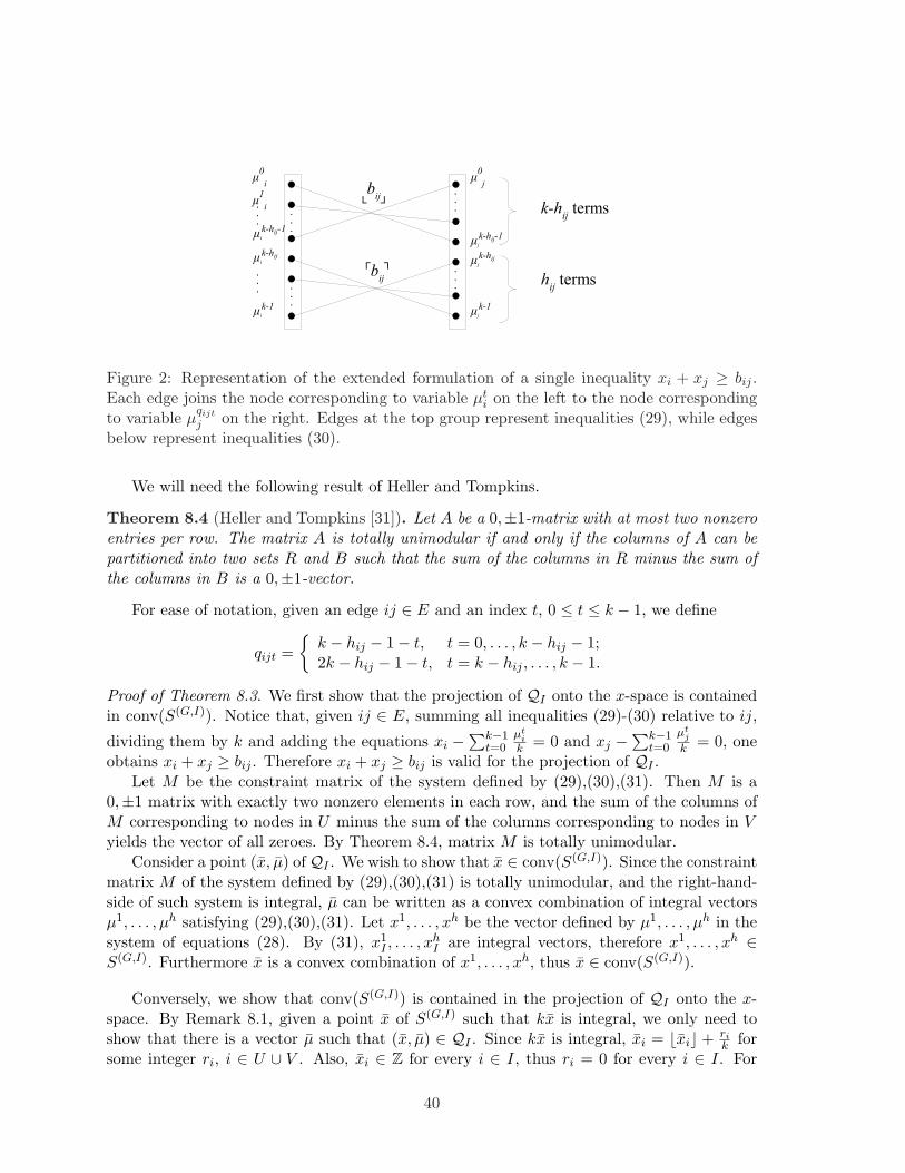
Figure 2: Representation of the extended formulation of a single inequality xi + xj ≥ bij .Each edge joins the node corresponding to variable µt

i on the left to the node correspondingto variable µ

qijt

j on the right. Edges at the top group represent inequalities (29), while edgesbelow represent inequalities (30).

We will need the following result of Heller and Tompkins.

Theorem 8.4 (Heller and Tompkins [31]). Let A be a 0,±1-matrix with at most two nonzeroentries per row. The matrix A is totally unimodular if and only if the columns of A can bepartitioned into two sets R and B such that the sum of the columns in R minus the sum ofthe columns in B is a 0,±1-vector.

For ease of notation, given an edge ij ∈ E and an index t, 0 ≤ t ≤ k − 1, we define

qijt =

k − hij − 1− t, t = 0, . . . , k − hij − 1;2k − hij − 1− t, t = k − hij , . . . , k − 1.

Proof of Theorem 8.3. We first show that the projection of QI onto the x-space is containedin conv(S(G,I)). Notice that, given ij ∈ E, summing all inequalities (29)-(30) relative to ij,

dividing them by k and adding the equations xi −∑k−1

t=0µt

ik = 0 and xj −

∑k−1t=0

µtj

k = 0, oneobtains xi + xj ≥ bij . Therefore xi + xj ≥ bij is valid for the projection of QI .

Let M be the constraint matrix of the system defined by (29),(30),(31). Then M is a0,±1 matrix with exactly two nonzero elements in each row, and the sum of the columns ofM corresponding to nodes in U minus the sum of the columns corresponding to nodes in Vyields the vector of all zeroes. By Theorem 8.4, matrix M is totally unimodular.

Consider a point (x, µ) ofQI . We wish to show that x ∈ conv(S(G,I)). Since the constraintmatrix M of the system defined by (29),(30),(31) is totally unimodular, and the right-hand-side of such system is integral, µ can be written as a convex combination of integral vectorsµ1, . . . , µh satisfying (29),(30),(31). Let x1, . . . , xh be the vector defined by µ1, . . . , µh in thesystem of equations (28). By (31), x1

I , . . . , xhI are integral vectors, therefore x1, . . . , xh ∈

S(G,I). Furthermore x is a convex combination of x1, . . . , xh, thus x ∈ conv(S(G,I)).

Conversely, we show that conv(S(G,I)) is contained in the projection of QI onto the x-space. By Remark 8.1, given a point x of S(G,I) such that kx is integral, we only need toshow that there is a vector µ such that (x, µ) ∈ QI . Since kx is integral, xi = bxic + ri

k forsome integer ri, i ∈ U ∪ V . Also, xi ∈ Z for every i ∈ I, thus ri = 0 for every i ∈ I. For

40

every i ∈ U ∪ V , define µti = bxic for t = 0, . . . , k − ri − 1, µt

i = dxie for t = k − ri, . . . , k − 1.Clearly (x, µ) satisfies (28) and (31). We now show that µ satisfies (29),(30). In fact, givenij ∈ E and an index t, 0 ≤ t ≤ k − 1, observe that the vector µ defined above satisfies

1k(µ0

i + . . . + µk−1i ) +

1k(µ0

j + . . . + µk−1j ) ≥ bij ;

1kµt

i −1kµ`

i ≥ 0, ` = 0, . . . , t− 1;

1kµt

i −1kµ`

i ≥ − 1k , ` = t + 1, . . . , k − 1;

1kµ

qijt

j − 1kµ`

j ≥ 0, ` = 0, . . . , qijt − 1;

1kµ

qijt

j − 1kµ`

j ≥ − 1k , ` = qijt + 1, . . . , k − 1.

Summing all these inequalities, we obtain

µti + µ

qijt

j ≥ bij − 1k(2k − 2− t− qijt).

For t = 0, . . . , k−hij−1, this gives µti+µ

qijt

j ≥ bij−1− 1k (hij−1), that is µt

i+µqijt

j ≥ bbijc−1+ 1k .

Since µ is integral, it satisfies (29).For t = k−hij , . . . , k−1, this gives µt

i+µqijt

j ≥ bij− 1k (hij−1), that is µt

i+µqijt

j ≥ bbijc+ 1k .

Since µ is integral, it satisfies (30).2

Remark 8.5. Observe that constraints (31) are equivalent to xi = µ1i = . . . = µk−1

i for i ∈ I.Therefore, for i ∈ I, the variables µt

i, t = 0, . . . , k−1 can be eliminated in the system definingQI by replacing them with variable xi. The constraint matrix of the system obtained from(29),(30), ij ∈ E, by the above substitution is again totally unimodular.

Example. The mixing set [42] is the set

XMIXn = (x0, x) ∈ R× Zn : x0 + xi ≥ bi, i = 1, . . . , n.

Let bi = hik , i = 1, . . . , n, where k and h1, . . . , hn are integer. After replacement of each

variable µti, i = 1, . . . , k, t = 0, . . . , k − 1 by the variable xi as explained in Remark 8.5, the

extended formulation for conv(XMIXn ) given in Theorem 8.3 becomes

kx0 − µ00 − · · · − µk−1

0 = 0,µt

0 + xi ≥ bbic, t = 0, . . . , k − hi − 1, i = 1, . . . , n;µt

0 + xi ≥ dbie, t = k − hi, . . . , k − 1, i = 1, . . . , n.

Figure 3 depicts the constraints defining XMIXn and the corresponding extended formu-

lation. ¥

Remark 8.6. The extended formulation in Theorem 8.3 has O(k|U ∪ V |) variables andO(k|E|) constraints. Therefore its size is pseudopolynomial, but in general not polynomial, inthe size of the encoding of S(G,I). In fact one can construct counterexamples to polynomiality[14].

41

Figure 3: Mixing set and extended formulation.

The extended formulation in Theorem 8.3 can be turned into a formulation of polynomialsize whenever we have the property that every point in conv(S(G,I)) can be expressed asconvex combination of points of S(G,I) in which the fractional parts of the coordinates ofthese points can take only “a small number” of possible values. More formally.

Remark 8.7. Suppose we are given L ⊂ 0, . . . , k − 1 with the property that

conv(S(G,I)) = conv(S(G,I) ∩ x : k(xi − bxic) ∈ L).

(By Lemma 8.1, the set 0, . . . , k − 1 has the above property.)The extended formulation presented in Section 2 can be turned into an extended formula-

tion of size polynomial in |L| by setting µti = µt−1

i whenever k − t 6∈ L and then eliminatingvariables and duplicate constraints.In particular, whenever such a set |L| is known whose size is polynomial in the input data,this yields a polynomial size extended formulation.

Conforti et al. [14] give bounds on the smallest size of a set L satisfying the conditions ofRemark 8.7. Given any such set L, they also give an extended formulation for conv(S(G,I))that has |L||V (G)| additional variables. It can be seen that such an extended formulationis that given in Remark 8.7, with the additional constraints µt

i − µt−1i ≥ 0, t = 1, . . . , k − 1,

µ0i − µk−1

i ≥ −1.

9 Conclusion

This survey presented a number of tools for deriving and studying extended formulations:Projection, Minkowski-Weyl, union of polyhedra, dynamic programming, and variable dis-cretization. In each case, we showed how to use the tool in one or several applications. Atheorem of Yannakakis gives a lower bound on the size of an extended formulation. Thisresult does not seem to be well known and it certainly deserves greater recognition.

Acknowledgments: We thank Marco DiSumma for his valuable comments.

42

References

[1] M. Ajtai, J. Komlos, E. Szemeredi, An O(n log n) sorting network, Proceedings of the15th Annual ACM Symposium on Theory of Computing (1983), 1–9.

[2] N. Alon, R. Yuster, U. Zwick. Color-coding, Journal of the ACM 42 (1995), 844856.

[3] D. Avis, K. Fukuda, A pivoting algorithm for convex hulls and vertex enumeration ofarrangements and polyhedra, Discrete Computational Geometry 8 (1992), 295-313.

[4] E. Balas, Disjunctive programming: properties of the convex hull of feasible points,GSIA Management Science Research Report MSRR 348, Carnegie Mellon University(1974), published as invited paper in Discrete Applied Mathematics 89 (1998) 1–44.

[5] E. Balas, Disjunctive programming and a hierarchy of relaxations for discrete optimiza-tion problems, SIAM Journal on Algebraic and Discrete Methods 6 (1985) 466–486.

[6] E. Balas and W. R. Pulleyblank, The perfectly matchable subgraph polytope of a bi-partite graph, Networks 13 (1983), 495-516.

[7] E. Balas and W. R. Pulleyblank, The perfectly matchable subgraph polytope of anarbitrary graph, Combinatorica 9 (1989), 321-337.

[8] F. Barahona, On cuts and matchings in planar graphs, Mathematical Programming 60(1993), 53–68.

[9] F. Barahona, Reducing matching to polynomial size linear programming, SIAM Journalof Optimization 3 (1993), 688–695.

[10] D. Bienstock, Approximate formulations for 0 − 1 knapsack sets, Operations ResearchLetters 36 (2008) 317–320.

[11] D. Bienstock, B. McClosky, Tightening simple mixed-integer sets with guaranteedbounds, (2008), manuscript. http://www.caam.rice.edu/ bjm4/ak.pdf

[12] R. Carr, G. Konjevod, G. Little, V. Natarajan, O. Parekh, Compacting cuts: a new linearformulation for minimum cut, Proceeding of the Symposium on Discrete Algorithms(2007), 43-52.

[13] M. Conforti, G. Cornuejols and G. Zambelli, Polyhedral Approaches to Mixed IntegerLinear Programming, in 50 Years of Integer Programming 1958-2008, Springer BerlinHeidelberg (2009) 343–385.

[14] M. Conforti, M. Di Summa, F. Eisenbrand, L.A. Wolsey, Network formulations of mixed-integer programs, Mathematics of Operations Research 34 (2009) 194-209.

[15] M. Conforti and L. Wolsey, Compact formulations as a union of polyhedra, MathematicalProgramming 114 (2008), 277-289.

[16] M. Conforti, L. Wolsey and G. Zambelli, Projecting an extended formu-lation for mixed-integer covers on bipartite graphs, working paper (2008).www.math.unipd.it/ giacomo/papers/mix-tree.pdf

[17] T.H. Cormen, C.E. Leiserson, R.L. Rivest, C. Stein, Introduction to Algorithms, MITPress, 2001.

[18] J. Edmonds, Maximum matching and a polyhedron with 0, 1-vertices, Journal of Re-search National Bureau of Standards Section B 69 (1965) 125-130.

43

[19] J. Edmonds, Submodular functions, matroids, and certain polyhedra, in CombinatorialStructures and Their Applications (Proceedings Calgary International Conference onCombinatorial Structures and Their Applications, Calgary, Alberta, 1969; R. Guy, H.Hanani, N. Sauer, J. Schonheim, eds.), Gordon and Breach, New York, 1970, 69–87.

[20] J. Edmonds, Matroids and the greedy algorithm, Mathematical Programming 1 (1971)127–136.

[21] J. Edmonds, Edge-disjoint branchings, in Combinatorial Algorithms (Courant ComputerScience Symosium 9, Monteray, California, 1972; R. Rustin, ed.), Algorithmic Press, NewYork, 1973, 91-96.

[22] J. Edmonds, E.L. Johnson, Matching, Euler tours and the Chinese postman, Mathemat-ical Programming 5 (1973) 88–124.

[23] Y. Faenza, V. Kaibel, Extended Formulations for Packing and Partitioning Orbitopes,Mathematics of Operations Research 34 (2009) 686-697.

[24] J.B.J. Fourier, Solution d’une question particuliere du calcul des inegalites, NouveauBulletin des Sciences par la Societe Philomatique de Paris (1826) 317–319.

[25] D. R. Fulkerson, Blocking polyhedra, in: Graph Theory and its Applications, (Proceed-ings Advanced Seminar Madison, Wisconsin, (1969); B. Harris ed.), Academic Press,New York, (1970) 93-112.

[26] B. Gerards, Compact systems for T-join and perfect matching polyhedra of graphs withbounded genus, Operations Research Letters 10 (1991) 377-382.

[27] R. Giles and L. Trotter Jr., On the stable set polytope for K1,3-free graphs, Journal ofCombinatorial Theory B 31 (1981) 313–326.

[28] M.X. Goemans, Smallest compact formulation for the permutahedron, working paper,MIT Department of Mathematics, 2010.

[29] B. Guenin, A characterization of weakly bipartite graphs, Jounal of Combinatorial The-ory B 83 (2001) 112–168.

[30] O. Gunluk and Y. Pochet, Mixing mixed-integer inequalities, Mathematical Programming90 (2001) 429–458.

[31] I. Heller and C.B. Tompkins, An extension of a theorem of Danzig’s , in Linear Inequal-ities and Related Systems (H. W. Kuhn and A. W. Tucker, eds.) Princeton UniversityPress, Princeton, N.J., 1956, pp. 247-254.

[32] A. J. Hoffman and J. B. Kruskal, Integral boundary points of polyhedra, in: LinearInequalities and Related Systems (H. W. Kuhn and A. W. Tucker eds.), Princeton Uni-versity Press, Princeton, N.J. (1956) 223–246.

[33] O.H. Ibarra, C.E. Kim, Fast approximation algorithms for the knapsack and sum ofsubset problems, Journal of the ACM 22 (1975) 463–468.

[34] R. Jeroslow, On defining sets of vertices of the hypercube by linear inequalities, DiscreteMathematics 11 (1975) 119-124.

[35] V. Kaibel, K. Pashkovich, D.O. Theis, Symmetry matters for sizes of extended formula-tions, accepted in IPCO 2010.

44

[36] V. Kaibel, M.E. Pfetsch, Packing and partitioning orbitopes, Mathematical ProgrammingA 114 (2008) 1-36.

[37] R.M. Karp, Reducibility among combinatorial problems, in: Complexity of ComputerComputations (R.E. Miller and J.W. Thatcher eds.), Plenum Press, New York (1972)85–103.

[38] E.L. Lawler, Fast approximation algorithms for knapsack problems, Symposium on Foun-dations of Computer Science (1977) 206–213.

[39] R.R. Meyer, On the Existence of Optimal Solutions to Integer and Mixed Integer Pro-gramming Problems, Mathematical Programming 7 (1974) 223-235.

[40] A. Miller and L.A. Wolsey, Tight formulations for some simple MIPs and convex objectiveIPs, Mathematical Programming B 98 (2003) 73–88.

[41] M.W. Padberg, M.R. Rao, Odd minimum cut-sets and b-matchings, Mathematics ofOperations Research 7 (1982) 67-80.

[42] Y. Pochet and L.A. Wolsey, Polyhedra for lot-sizing with Wagner-Whitin costs, Mathe-matical Programming 67 (1994) 297–324.

[43] Y. Pochet and L.A. Wolsey, Production Planning by Mixed Integer Programming,Springer Series in Operations Research and Financial Engineering, New York, 2006.

[44] W. R. Pulleyblank and F. B. Shepherd, Formulations for the stable set polytope, Pro-ceedings of IPCO III (eds. G. Rinaldi, L.A. Wolsey), Springer, Berlin, 1993, pp. 267-279.

[45] A. Schrijver, Theory of Linear and Integer Programming, Wiley, New York (1986).

[46] A. Schrijver, Combinatorial Optimization, Polyhedra and Efficiency, Springer, Berlin(2003).

[47] P.D. Seymour, Sums of circuits, in Graph Theory and Related Topics (J.A. Bondy andU.S.R. Murty, eds), Academic Press, New York, 1979, 341-355.

[48] M. Van Vyve, The continuous mixing polyhedron, Mathematics of Operations Research30 (2005) 441–452.

[49] M. Van Vyve, L.A. Wolsey, Approximate extended formulations, Mathematical Program-ming 105 (2006) 501–522.

[50] M. Yannakakis, Expressing combinatorial optimization problems by linear programs,Journal of Computer and System Sciences 43 (1991) 441–466.

[51] G.M. Ziegler, Lectures on Polytopes, Springer, New York (1995).

45