EXPORTING LIQUIDITY:

BRANCH BANKING AND FINANCIAL INTEGRATION*

Erik Gilje, The Wharton School, University of Pennsylvania

Elena Loutskina, University of Virginia, Darden School

Philip E. Strahan, Boston College and NBER

August 2014

ABSTRACT

Using exogenous liquidity windfalls from oil and natural gas shale discoveries, we demonstrate that bank branch networks help integrate U.S. lending markets. Banks exposed to shale booms enjoy liquidity inflows, thereby increasing their capacity to originate and hold new loans. Exposed banks increase mortgage lending in non-boom counties, but only where they have branches and only for hard-to-securitize mortgages. Our findings suggest that contracting frictions limit the ability of arm’s length finance to integrate credit markets fully. Branch networks continue to play an important role in financial integration, despite the development of securitization markets.

*We thank seminar participants at University of Amsterdam, ESSEC, Georgetown, The Federal Reserve Bank of New York, University of Houston, INSEAD, University of Michigan, Ohio State, DePaul University, University of Oklahoma, University of Virginia, University of Rotterdam, Rice, SMU, and Tilburg University. We also thank the conference participants and our discussants (Mark Carey, Christopher James, Justin Murfin, Greg Nini, Amit Seru, and James Vickery) at the Financial Intermediation Research Society Conference, the Western Finance Association Conference, the SFS Cavalcade Conference, New York Fed/NYU Stern Conference on Financial Intermediation, and Bank Structure and Competition Conference of the Chicago Federal Reserve.

1

I. INTRODUCTION

Over the past thirty years the banking system in the U.S. has gone through a significant

transformation, relying more on capital markets and direct finance in funding loans and less on

local bank deposits. The U.S. mortgage market has been at the forefront of this transformation,

with 52% of loans in 2011 financed by securitization markets, up from 12% in 1980.1 Moreover,

improvements in information technology have facilitated bank lending well outside of branch-

based geographical domains (Petersen and Rajan, 2002). These changes have allowed capital to

flow across the U.S. economy and thus integrate local credit markets. The greater role of

external capital markets in facilitating access to credit should have diminished the value of bank

branch networks for lending. Yet over the same period the extent and density of bank offices

and branches has continued to grow, from 63,200 (about 5 per bank) in 1990 to 89,800 (about 14

per bank) in 2012.2

In this paper, we show that branch networks still play an important role in integrating

local credit markets. Using a unique positive exogenous shock to bank liquidity stemming from

oil and gas “fracking” booms, we document that bank liquidity inflows increase mortgage

lending in areas not experiencing the booms. Lending increases only in markets where banks

have a branch presence. The effect is most pronounced for loan types that are subject to more

contracting frictions, and therefore are harder to fund from external markets (e.g., through

securitization). Moreover, banks exposed to shale-booms expand overall lending, as opposed to

merely taking lending business away from other banks operating in similar markets. Combined,

the results provide evidence that branch networks allow lenders to mitigate contracting frictions,

1 These statistics refer to the whole mortgage market, including mortgages for home purchase, home equity lines, as well as mortgage re-financings.

2 See http://www2.fdic.gov/hsob/HSOBRpt.asp.

2

and thus play an important role in integrating information intensive segments of credit markets

where arm’s length financing is limited.

To identify how funds flow across markets, we exploit a unique bank liquidity shock

stemming from “fracking” booms ̶ the unexpected technological breakthrough that made vast

amounts of shale oil and gas deposits economically profitable to develop. Oil and gas companies

pay significant mineral royalty payments to landowners to develop shale resources. This wealth

windfall results in increased deposit supply for banks with branches in shale-boom counties

(Gilje, 2011 and Plosser, 2011). It also allows local landowners to pay down outstanding debt,

further amplifying banks’ liquidity windfalls.

Armed with this exogenous shock, we evaluate whether banks export liquidity by

focusing on mortgage originations outside of shale-boom counties. Exploring mortgage lending

has three advantages. First, these loans have a clear geographical dimension pinned down by the

property location, which is not possible for other types of loans. Second, studying lending

outside shale boom counties alleviates concerns that shale discoveries drive credit demand.

Third, the rich dataset allows us to saturate models with county*year fixed effects, thus removing

confounding demand effects. Conceptually, our analysis compares mortgage growth rates in the

same county-year for two otherwise similar banks, one with branches in a shale-boom county

(and thus exposed to a positive liquidity shock) and the other without exposure.

Why might local liquidity shocks affect credit? The traditional banking literature argues

that two frictions are necessary for a liquidity shock to propagate. First, banks must face

(liability-side) frictions in accessing external financing that preclude them from undertaking all

profitable investment opportunities. In our setting, this friction stems from small and regional

banks having limited access to external debt and equity markets and drawing most of their funds

3

from insured (and potentially subsidized) deposits. These regional banks are at the center of our

analysis, as they benefit most from the fracking wealth windfalls. 3 We show that shale booms

lead to a simultaneous increase in quantity and decline in cost of deposits at banks with branches

in the shale-boom counties. The lower financing costs thus allow them to expand their

investments in either loans or marketable securities.

For the shock to stimulate new lending, a second (asset-side) friction between banks and

borrowers is required: some new lending made by banks with liquidity inflows must be ones that

other banks would not choose to originate. Thus, for new lending to be stimulated, we need

banks to have access to a set of borrowers over which they have a cost advantage relative to

competing banks. A bank’s physical branch footprint provides such an advantage, as

geographical proximity lowers the cost of information production and allows better loan

monitoring (e.g., Berger et al., 2005). Thus, banks would expand new credit in markets where

they possess local information or a borrower relationship advantage.

Our results indicate that banks export newly found liquidity to other markets. An average

bank exposed to the boom grows its mortgage originations 7% faster relative to a similar non-

exposed bank. This effect is large relative to average mortgage origination growth rates (11%).

Furthermore, consistent with the notion that bank branches mitigate contracting frictions,

mortgage lending increases only in outlying (non-boom) counties where exposed banks have

branches. Lending does not increase in areas where exposed banks have no local knowledge and

thus have no informational advantage over other sources of financing (e.g. securitization). To

further solidify this notion, we document that liquidity windfalls expand lending more in loan

3 Our experiment is not likely to matter for very large banks, in part because such banks have relatively easy access to the interbank market, meaning that the marginal cost of funds is unlikely to be affected by a small shock to the deposit base. In fact, when we exclude the largest banks from our tests the coefficients of interest do not change (see Table 5).

4

types subject to greater contracting frictions, which are less likely to be securitized, such as home

equity lines (sold or securitized 4.5% of the time) and home-purchase mortgage (sold or

securitized 46% of the time), as opposed to mortgage re-financings (sold or securitized 65% of

the time). Overall, our evidence suggests that bank branches integrate segments of lending

markets that arm’s-length finance cannot.

Our core results leave the question of efficiency in allocation of newly found liquidity

unanswered. Perhaps exposed banks waste the proceeds of the shale booms on pet projects

(<NPV), as in Jensen (1986). One might even argue that such pet projects are most likely to be

located near a bank’s branches. We find no evidence supporting this agency problem. Loan

delinquencies and charge-offs of banks exposed to shale booms fall rather than rise after the

exposure to the boom, with varying degrees of statistical significance that depend on the ex-post

horizon and model specification.

Our findings contribute to several strands of the literature. First, the results extend

research on the financial integration of U.S. markets and help explain why large benefits

followed deregulation.4 Two mechanisms, potentially working in parallel, can explain why the

removal of restrictions on banks’ ability to expand across geographical markets improved

economic outcomes: tougher competition and improved capital mobility. There is abundant

evidence that increases in competition post-deregulation led to more efficient banking (Stiroh

and Strahan, 2003), lowered the cost of capital for non-financial firms (Rice and Strahan, 2010)

4 The intrastate branching deregulation led to faster growth of the state economies (Jayaratne and Strahan (1996)) and lower growth volatility (Morgan, Rime and Strahan (2004)). Such deregulation came with better quality lending (Jayaratne and Strahan, 1996), more entrepreneurship and a greater share of small establishments (Black and Strahan 2002; Cetorelli and Strahan, 2006, Kerr and Nanda, 2009), lower income inequality, less labor-market discrimination and weaker labor unions (Black and Strahan, 2001; Beck et al., 2010; Levkov, 2012). That said, Loutskina and Strahan (forthcoming) provide evidence from the recent housing boom that financial integration helped fuel local housing and economic booms, thus raising local volatility.

5

and contributed to better allocation of resources (Jayaratne and Strahan, 1996). There is much

less direct evidence, however, about deregulation’s effect on capital mobility. In this paper, we

show that branch networks contribute to capital flows across local credit markets. Thus, the

increasing scope and density of bank branch networks made possible by deregulation potentially

increased the efficiency of capital allocation by allowing savings in one area to finance

investment in other areas.

Second, extant research evaluates whether close proximity between borrowers and

lenders lowers the cost of information production and monitoring. Breakthroughs in information

technology allowed for larger distances between borrowers and lenders (Petersen and Rajan,

2002). However, local lenders still extend more credit to riskier borrowers than distant lenders:

loan rates tend to decline with the distance between borrower and lender (Degryse and Ongena,

2005; Agrawal and Hauswald, 2010); more opaque (smaller) borrowers tend to establish

enduring relationships with their local (small) banks; and larger, more transparent firms tend to

borrow from larger (not so local) financial intermediaries (e.g., Berger et al., 2005). In mortgage

finance, locally concentrated lenders focus on soft information intensive segments of the

mortgage market (Loutskina and Strahan, 2011) and have an advantage in screening and

monitoring riskier borrowers (Cortes, 2011). We contribute to this literature by documenting

that even in the most developed, integrated, and technologically advanced lending market ̶ the

U.S. mortgage market ̶ local finance is hard to substitute. Branch networks, and by extension

local knowledge, remain important for segments of the credit markets subject to contracting

frictions.

6

Third, our paper offers a micro-economic approach to testing the bank lending channel. 5

Most of the existing studies exploit a common bank liquidity shock engineered by a central bank.

These shocks naturally correlate strongly with credit demand and business cycle conditions,

creating identification challenges. Some studies address these challenges by exploiting cross-

sectional differences in bank on-balance-sheet lending responses to aggregate liquidity shocks

(e.g., Gertler and Gilchrist, 1994, Kashyap et al., 1994, Kashyap, Stein, 2000, Campello, 2002

and Loutskina, 2011). Other more recent studies use natural experiments, where external shocks

from abroad propagate into domestic credit markets through cross-border ownership of banks

(e.g., Peek and Rosengren, 1997, Schnabl, 2012, Cetorelli and Goldberg, 2012). Our study is

closest to those evaluating how local liquidity shocks from bank failures, government

interventions or bank runs affect lending supply (Ashcraft, 2006, Khwaja and Mian, 2008,

Paravisini, 2008, Iyer and Peydro, 2011). Unlike much of the earlier literature, however, we

isolate the supply effects by exploiting data with precise information on the location of both

lender and borrower location.

In the remainder of the paper, Section II describes briefly the shale booms and their

effects on local banks. Section III contains a simple conceptual framework to motivate our tests.

Section IV describes our data, and Section V reports empirical methods and results. Section VI

contains a brief conclusion.

II. SHALE BOOMS

In 2003, a surprise technological breakthrough combined horizontal drilling with

hydraulic fracturing (“fracking”) and enabled development of natural gas shale. The subsequent

5 See the theoretical arguments in, e.g., Bernanke and Blinder (1988), Holmstrom and Tirole (1997), and Stein (1998).

7

development of shale led to a new energy resource equivalent to 42 years of U.S. motor gasoline

consumption. As recently as the late 1990s, shale gas was not thought to be economically viable,

and represented less than 1% of U.S. natural gas production. The development of the Barnett

Shale near Fort Worth, TX in 2003 changed industry notions on the viability of natural gas shale.

The Barnett Shale was initially drilled by Mitchell Energy in the early 1980s (Yergin,

2011). Rather than encountering the highly porous rock of a conventional formation, however,

Mitchell encountered natural gas shale. While shale holds vast amounts of natural gas, it is

highly non-porous and traps the gas in the rock. After 20 years of experimentation, in the early

2000s Mitchell Energy found that hydraulic fracturing (“fracking”) could break apart shale and

free natural gas for collection at the surface. This breakthrough combined with horizontal

drilling and higher natural gas prices made large new reserves from shale economically

profitable to develop.

The size of this energy resource and the low risk of unproductive wells (“dry-holes”)

have led to a land grab for mineral leases. Before commencing any drilling operations, oil and

gas firms must negotiate leases with mineral owners. Typically these contracts are comprised of

a large upfront “bonus” payment, paid whether the well is productive or not, plus a royalty

percentage based on the value of the gas produced over time. The resulting wealth windfalls led

to large increases in local bank deposits. In an interview with the Houston Chronicle (2012),

H.B. “Trip” Ruckman III, president of a bank in the Eagle Ford shale, stated “We have had

depositors come in with more than a million dollars at a whack.” This statement is consistent

with reports of leasing terms. For example, an individual who owns one square mile of land

(640 acres) and leases out his minerals at $10,000/acre would receive an upfront one-time

8

payment of $6.4 million plus a monthly payment equal to 25% of the value of all the gas

produced on his lease.

Two previous studies have tested how the shale booms affected banks and bank lending,

as well local real outcomes. Plosser (2011) studies the impact on banks, finding that exposure to

shale booms comes with increased bank lending as well as holdings of securities. These results

are consistent with the idea that bank financing costs fall with the advent of shale booms. Gilje

(2011) studies outcomes for non-financial firms within shale-boom counties themselves, finding

that financially dependent industries grow relative to less dependent ones; he argues that greater

credit supply within the booming areas stimulated investment. Neither study, however, explores

the implications of the shale booms for outlying markets connected via branch networks, as ours

does.

The shale-boom windfalls represent an exogenous liquidity shock relative to the

underlying characteristics of the affected communities for a number of reasons. First, the

economic viability of shale wells was determined by larger macroeconomic forces, such as

demand for natural gas and natural gas prices (Lake, Martin, Ramsey, and Titman, 2012), and

therefore was unrelated to the local economic conditions (health, education, demographics, etc.).

Second, the technological breakthroughs, horizontal drilling and hydraulic fracturing,

were unexpected, and the viability of these technologies in different geographies was uncertain.

It was extremely challenging even for oil and gas companies to predict how many wells an area

might need to develop recoverable resources. Highlighting the fast pace and unpredictable

nature of these discoveries, in 2008, five years after the technology was discovered, the

Haynesville Shale area in Louisiana experienced an increase in lease bonus payments from a few

9

hundred dollars an acre to $10,000 to $30,000 an acre within a one-year time period (reported by

the New Orleans' Times-Picayune, 2008).

Combined, these facts suggest that it was unlikely that banks could strategically alter

branch structures to gain greater exposure to shale liquidity windfalls. Thus, bank windfalls

from shale discoveries are an attractive setting to study how liquidity is exported across branch

networks in the U.S.

III. CONCEPTUAL FRAMEWORK

We evaluate the anatomy of the financial integration of the U.S. mortgage markets

through the prism of the lending channel, where shocks to bank financing costs affect their

lending. In the frictionless world of Modigliani and Miller, the cost or availability of firm

financing should have no effect on investment. Yet the corporate finance literature argues, for

example, that cash-flow shocks raise investment by alleviating frictions of raising funds in

external markets. Similarly, the bank lending channel needs frictions so that liquidity shocks

propagate and affect investment. These frictions originate on both the liability and asset sides of

bank balance sheets. To illustrate these ideas, below we offer a simple conceptual framework to

motivate our empirical tests.

Liability-Side Response to Shale-Booms

Banks face frictions in tapping external capital markets that sometimes make external

finance expensive or even unavailable, limiting their ability to finance all positive NPV projects.

Existing literature argues that smaller banks face significantly greater frictions than larger ones

in accessing external sources of finance such as the interbank market or the bond market. Thus,

small banks respond more, for example, to central bank policy shocks (Kashyap and Stein, 2000;

10

Jayaratne and Morgan, 2000; Campello, 2002). Constrained banks face an upward sloping

supply of funds that tops out at the rather high external borrowing rate (illustrated in Figure 1A).

In contrast, very large, publicly owned banks (e.g. Bank of America) would have much better

and cheaper access to external finance, so their cost of funds would flatten quickly and at a lower

level (Figure 1B). The marginal cost of funds for such very large banks might be pinned down

by the interbank borrowing rate (e.g. the Federal Funds rate).

Deposit windfalls and loan repayments stemming from shale booms reduce the marginal

cost of funds for banks with substantial business in booming areas, illustrated in Figure 1. Since

location provides convenience to nearby depositors (Pilloff and Rhoades, 2002) and borrowers

(Berger et al., 2005), banks with branches in the booming counties have an advantage in

harvesting local landowners’ wealth windfalls. These banks’ cost of funds would fall with the

advent of liquidity shocks generated by additional deposit inflows (which we document below)

and/or loan prepayments (which are not observable because loan balances combine old and new

loans).

Asset-Side Response

A mere shift in banks’ cost of funding is not sufficient to affect lending. Banks with low

cost funds may simply take business away from competing banks with higher cost funds, or they

may expand their holdings of marketable securities. For lending to change, we need each bank

to serve a portion of borrowers over which it possesses better information (i.e. lower screening

and monitoring costs) than potential competitors. With access to a pool of such borrowers, each

bank will face a declining marginal return on lending. These returns will bottom out and flatten

once the marginal investment becomes a marketable security (or, in this context, a mortgage that

could potentially be made by any other lender, which itself would be securitizable).

11

With some degree of market power over a set of borrowers, the decline in funding costs

from shale booms allows banks to originate and hold previously unprofitable loans. As

presented in Figure 1A, the bank thus will increase the amount lent (moving from point A to

point B) when funding costs fall. Banks facing relatively weak loan demand would expand their

holdings of marketable securities rather than loans (Figure 1C). Loan-market power plausibly

stems from informational advantages in screening and monitoring, which each bank uniquely

possess based on local knowledge from close proximity to borrowers (Degryse and Ongena,

2005; Loutskina and Strahan, 2011). Moreover, mortgage credit availability for low-income

borrowers increases with bank branch presence, and both interest rates and defaults are lower

(Ergungor, 2010; Ergungor and Moulton, forthcoming).

We recognize that this simple framework, taken literally, would imply that banks holding

marketable securities during the pre-boom period would not respond to the liquidity inflows.

But a more realistic framework would account for the idea that holding loans and taking deposits

exposes banks to liquidity risk; managing such risk requires banks to hold marketable securities

and cash (Kashyap, Rajan and Stein, 2002). In fact, Plosser (2011) shows that banks exposed to

shale booms increase both loans and securities.

Empirical Implications

This simple conceptual framework helps guide our empirical approach. First, we

compare lending responses in areas where banks plausibly have access to local knowledge –

markets where they have a branch presence – with responses in markets where they lend but

have no physical presence. In markets with branches, banks will face declining marginal returns

on new loan originations and also be forced to use internal funds rather than capital markets to

fund those loans. This follows directly because the information frictions that motivate lending

12

market power also create a barrier to securitization. Second, we segregate the mortgage

origination rates by the information sensitivity of the loan itself; information-sensitive loans (e.g.

subordinated second-lien mortgages) ought to respond more than less-information sensitive loans

(e.g. senior first-lien mortgages). Third, the response of loan originations ought to be stronger in

markets with more unsatisfied demand (compare Figures 1A and 1C). Thus, we separate our

data by local credit demand measured by lagged mortgage approval rates.

Our simple framework also suggests that large banks with access to public debt and

equity markets ought to respond less to liquidity inflows compared to small and regional banks

(compare Figures 1A and 1B). That said, we have little power in our empirical setting to test this

implication. Large banks not only have capital market access, they also have very extensive

branch networks. Our natural experiment – exposure to shale booms – is simply too small to

affect their liquidity in an empirically meaningful way for them. Bank of America, for example,

owned 6038 branches, 182 of which are located in shale-boom counties as of 2010 (~3%). In

contrast, the typical exposed bank in our sample has about 50% of its branches in a shale-boom

county.

Our tests are close to investment-cash flow studies in the corporate finance literature,

which imply that cash-flow shocks raise investment by alleviating the need to raise funds in

external markets. This literature began by exploring correlations between cash-flow shocks and

investment for different types of firms (Fazzari, Hubbard and Petersen, 1988). Subsequent

challenges to this approach emerged, however, because cash flow innovations may be correlated

with investment opportunities or because financial constraints may be measured with error (e.g.

Kaplan and Zingales, 1997; Alti, 2003). Our setting avoids these identification problems

because we can test how liquidity shocks affect lending in areas that are not the source of the

13

shock. Moreover, unlike studies of non-financial companies, investment by banks can be

separated into that which must be financed internally (mortgages over which the lender possesses

an information advantage) vs. investments that can be financed externally (mortgages that are

easily securitized).

IV. DATA AND SAMPLE SELECTION

Our sample is based on lending activity in the seven states with major shale discoveries

between 2003 and 2010: Arkansas, Louisiana, North Dakota, Oklahoma, Pennsylvania, Texas

and West Virginia. As Figure 2 shows, each state contains a large number of counties that

experienced shale booms as well as a large number of non-boom counties. Across the seven

states, 124 counties experienced booms and 515 did not. Our sample, built at the bank-county-

year level, includes all banks making housing-related loans (home purchase mortgages,

mortgages for re-financing, and home equity loans) in any of these seven states. We consider all

lenders irrespective of their branch locations (i.e., including loans originated without brick and

mortar presence in a county) or exposure to the booms. We drop all non-bank lenders because

most fund mortgage lending with securitization and are, thus, only affected by changes in the

aggregate supply of funds from the securitization market. The sample begins in 2000 (three

years before the first shale boom), and ends in 2010.

Using the Summary of Deposits from the Federal Insurance Deposit Corporation (FDIC),

we determine the number of branches and amount of deposits held by each bank in each county-

year in the seven states.6 These data allow us to build two alternative measures of exposure to

the shale-boom shocks. The first – Share of Branches in Boom Counties – equals the fraction of

6 http://www2.fdic.gov/sod/.

14

branches owned by each bank that are located in a shale-boom county. The measure ranges from

zero (for banks without branches in boom counties, or for banks with branches in boom counties

during the years prior to a boom’s onset) to one (for banks with all of their branches in boom

counties after the onset of the booms). This variable equals zero for all bank-years prior to 2003,

the year of the first shale investment. After 2003, the variable increases within bank over time as

more counties experience booms.

Our second measure accounts for both the distribution of branches across counties as well

as the size of the shale investments. This measure – Growth in Shale Well Exposure – equals the

weighted exposure to the growth in the number of shale wells, where the fraction of a bank’s

branches in each county serves as weights. This measure is harder to interpret than the Share of

Branches in Boom Counties because it need not vary between zero and one, but it accounts for

differences in the relative size and growth of the booms.

Our models focus on the effect of exposure to the shale boom on mortgage credit growth,

but we include other bank characteristics as control variables, each measured from the end of the

prior year. These variables include the following: Log of Assetst-1; Deposits/Assetst-1;

Cost of Depositst-1 (=interest expenses on deposits / total deposits); Liquid Assets / Assetst-1;

Capital / Assetst-1 (=Tier 1 capital/ assets); C&I Loans / Assett-1; Mortgage Loans / Assetst-1;

Net Income / Assetst-1; Loan Commitments / Assetst-1; and, Letters of Credits /Assetst-1. Data for

bank control variables come from year-end Call Reports. We merge Call Report and HMDA

following Loutskina and Strahan (2009).

Table 1 reports summary statistics for our two measures of banks’ exposure to the shale

well boom - Share of Branches in Boom Counties and Growth in Shale Well Exposure (Panel

A), as well as the lagged bank characteristics (Panel B), separated by whether or not the bank has

15

any exposure to a shale-boom county. Table 1 shows that exposed banks tend to be larger than

non-exposed banks and that their deposits grow faster and have lower cost, consistent with the

notion that exposure to the shale boom leads to increases in deposit supply. The marked

difference in asset size (log of assets) is a potential concern in our models because large banks

differ in many ways from smaller ones, so we will report robustness tests in which we filter out

larger banks.

To measure mortgage activity, we utilize the detailed data on mortgage applications

collected annually under the Home Mortgage Disclosure Act (HMDA). Whether a lender is

covered depends on its size, the extent of its activity in a Central Business Statistical Area

(CBSA), and the weight of residential mortgage lending in its portfolio.7 The HMDA data

include loan size, whether or not a loan was approved, as well as some information on borrower

characteristics. Using HMDA data, we measure mortgage origination growth by bank-county-

year. HMDA reports both the identity of the lender as well as the location of the property down

to the census-tract level. These are the only comprehensive data on lending by US banks that

allow researchers to locate borrowers geographically. In principle we would also like to test for

similar effects on other kinds of loans (especially loans to small businesses), but micro data at

loan level are not available outside of housing. HMDA also contains information on the purpose

of the loan (mortgage purchase loans, home-equity loans, and mortgage re-financings) and

whether the lender expects to sell or securitize the loan within one year of origination. We use

7Any depository institution with a home office or branch in a CBSA must report HMDA data if it has made a home purchase loan on a one-to-four unit dwelling or has refinanced a home purchase loan and if it has assets above $30 million. Any non-depository institution with at least ten percent of its loan portfolio composed of home purchase loans must also report HMDA data if it has assets exceeding $10 million. Consequently, HMDA data does not capture lending activity of small or rural originators. U.S. Census shows that about 83 percent of the population lived in metropolitan areas over our sample period and hence the bulk of residential mortgage lending activity is likely to be reported under the HMDA.

16

these data to test whether loans easier to finance in securitization markets respond less to the

local liquidity inflows that follow shale booms.

Table 1 reports summary statistics for mortgage growth rates, defined as the difference in

the log of mortgage originations, at both bank-year (Panel C) and bank-county-year (Panel D)

levels. For purposes of simple comparisons, we focus mainly on the summary statistics at the

bank-year level, since our main variables of interest vary only at that level; in our regressions, we

absorb variation across county-years with fixed effects. For the average exposed bank,

mortgages grow 11.7% per year, compared to 11.2% for non-exposed banks. This difference is

larger for retained mortgage growth, which averages 9.1% per year for exposed banks, compared

to 7.7% for non-exposed banks. These raw differences could be attributed to both the deposit

windfalls as well as to economic growth of the boom counties. We isolate these two effects in

our regressions. Note that the standard deviation in the mortgage growth rates is very high

relative to the mean, but much of this variation reflects time-series fluctuations stemming from

changes in interest rates (which alter re-financing rates drastically) as well as variation around

the housing boom (2004-2006) and bust (2006-2010) periods, which our data straddle.

HMDA also offers some borrower characteristics, which we use to build the following

control variables for all loans originated at the bank-county-year level: borrower and area

income, loan size-to-borrower-income ratio, percent women applicants, percent minority

applicants, and percent minority population in the area of loan applications. In all of our models

we control for the contemporaneous means of each of these borrower attributes across all loan

applications in a given bank-county-year.

17

V. METHODS AND RESULTS

Shale-Booms as a Positive Liquidity Shock

We first establish that banks exposed to shale-booms experience liquidity inflows. Such

inflows occur both because local mineral rights owners expand the local supply of deposits by

putting funds into local bank branches (which is directly observable), and because they pay back

outstanding loans (which is not).

To establish the first channel – that bank deposit supply increases with shale-boom

exposure – we report regressions of both deposit quantity (deposit growth) and price (interest

expense on deposits / deposits), as follows:

Deposit Growthi,t = γ1Bank Boom Exposurei,t + Control Variables + εi,t , (1a)

Interest Expense / Depositsi,t = γ2Bank Boom Exposurei,t + Control Variables + εi,t , (1b)

where the unit of analysis varies by bank i / year t. If shale-booms increase deposit supply, then

we expect γ1 > 0 and γ2 < 0. We include lags of bank characteristics as control variables, as well

as bank and year fixed effects. Standard errors are clustered by bank.

As shown in Table 2, deposit quantity increases and its price falls with bank shale

exposure, consistent with a positive supply shock. (These changes are consistent with those

illustrated in Figure 1.) To understand magnitudes, consider comparing a bank with average

exposure to shale (Share of Branches in Boom Counties = 0.45) to one with no exposure.

According to our estimates, exposed banks would experience deposit growth about 2.5

percentage points faster (column 1: 0.45*0.0567) and the interest expense on deposits would fall

by about 7 basis points (column 3: 0.45*-0.0015). These magnitudes line up well with the

differences in means between exposed and non-exposed banks in Table 1.

18

Table 2 also reports similar regressions for the bank capital/asset ratio and the return on

assets (ROA = net income/lagged assets). These results suggest the neither bank equity capital

nor ROA differ between exposed v. unexposed banks ex ante. Thus, other than bank size, the

two sets of banks appear comparable along some key observable characteristics.

Baseline Result

To evaluate how liquidity windfalls affect mortgage lending, we estimate a three-

dimensional panel regression of the growth in mortgage originations in non-shale counties on

each bank’s shale-boom exposure, as follows:

Mortgage Growthi,j,t = αj,t + β Bank Boom Exposurei,t +Borrower & Lender Controls + εi,j,t , (2)

where i indexes lenders, j indexes counties, and t indexes years. With this panel structure we can

absorb county*year effects (αj,t), thus removing time-varying, county-level demand-side shocks

related to business cycles, industry composition, housing demand, etc. To further separate

supply shocks from potentially confounding demand shocks, we include in our sample only

counties that did not experience a shale boom during the 2000-2010 period. As in Table 2, we

use two alternative measures of a bank’s exposure to the shale booms: Share of Branches in

Boom Counties and Growth in Shale Well Exposure. Unlike Mortgage Growth, both exposure

measures do not vary across counties for a given bank-year; hence we build standard errors by

clustering by bank throughout all of our results.

We use mortgage origination growth (the change in logs) as the dependent variable,

rather than the log level of mortgage originations or market share. By normalizing the dependent

19

variable by last year’s lending in a respective bank-county, we account for variation in the extent

of lending in a given county by a given bank.8

We then decompose Mortgage Growth into the growth in retained mortgages and the

growth in sold or securitized mortgages. This decomposition not only helps validate our

identification strategy, it also allows for a deeper understanding of capital supply to the mortgage

market. First, it allows us to document the true on-balance-sheet sensitivity of total lending to a

liquidity supply shock. Second, it allows us to evaluate whether the liquidity allows banks to

retain more loans at the expense of the secondary market. Finally, our core hypothesis posits that

in response to an exogenous liquidity shock banks expand soft-information intensive lending

and, by extensions, banks should not invest more in hard-information lending. Thus, evaluating

banks’ securitized loan originations allows us to evaluate our core hypothesis.

As shown in Table 3, we find significant positive effects of exposure to shale-booms on

both total mortgage growth (columns 1 & 2) and growth of retained mortgages (columns 3 & 4),

but no significant effect on sold-loan growth (columns 5 & 6). For retained mortgages, a typical

exposed bank (e.g. one with about 45% of its branches in a shale-boom county – recall Table 1)

would grow its retained-mortgage portfolio 14 percentage points (=0.45*0.325) faster in the non-

boom counties than a similar bank without exposure to the shale-boom windfalls (based on the

coefficient of interest in column 3). The results are also robust to whether or not we include the

bank-year lagged control variables, which collectively have little explanatory power.

8 In addition to the intensive margin, we explored the variation on the extensive margin, which our growth rate approach cannot address since we require positive lending in the prior year (not reported). We did not find that liquidity windfalls affect the extensive margin. This null result, we think, occurs because the liquidity shocks matter only in areas where banks have a branch presence (documented below), and banks almost always lend a non-zero amount in areas where they have branches. We have also tested whether mortgage acceptance rates vary with shale-boom exposure but find that they do not.

20

Do Banks Enter ‘Boom’ Counties to Chase Funds?

One concern may be that, after observing the advent of shale-boom discoveries in 2003,

banks enter shale-boom counties (or counties with known shale reserves) to raise low-cost

deposits. If such entry were motivated by the need to fund new loans, then our effects could be

driven by both supply and demand factors, thus invalidating our identification strategy. 9

We address this concern by testing whether banks with higher loan demand subsequently

increase their exposure by entering shale-boom counties. Specifically, we evaluate what share of

a bank’s boom exposure is attributed to its 2002 branch distribution and whether bank-specific

loan demand affects the remaining variation. The distribution of branches in 2002 could not

have been motivated by demand for funds because shale booms started unexpectedly in 2003.

We build the 2002-branch-network exposure proxies using only the time variation in county

shale booms (Share of 2002 Branches in Boom Countiesi,t and Growth in Exposure from 2002

Branchesi,t). These measures capture exposure to the boom that would have occurred if each

bank had held constant its 2002 branch network. We then run the following regressions:

Share of Branches in Boom Countiesi,t = γ1•Share of 2002 Branches in Boom Countiesi,t +

γ2•Mortgage Application Growthi,t-1 + γ3•Mortgage Application Growthi,t-2

+ Control Variables + εi,t , (3a)

and

Growth in Shale Well Exposure i,t = γ1•Growth in Exposure from 2002 Branchesi,t +

γ2•Mortgage Application Growthi,t-1 + γ3•Mortgage Application Growthi,t-2 + Control

Variables + εi,t , (3b)

9 For example, Ben-David, Palvia and Spatt (2013) report evidence of banks increasing demand for deposits (and hence prices) locally when they face higher loan demand in out-of-state markets connected through branches.

21

where the unit of observation varies by bank i / year t.

If banks’ exposure to the boom is solely due to the time variation in onsets of boom

throughout the counties, then we expect γ1 = 1. If banks facing higher loan demand (captured by

past loan application growth) enter booming markets to access cheap deposits, then we expect

γ2 > 0 and/or γ3 > 0. We estimate (3a) and (3b) over the 2003 to 2010 period because these are

the years when the shale booms occur. The sample contains all banks that originated mortgages

in at least one county in the seven states that experience shale booms.

Table 4 reports the estimates of (3a) in Panel A and (3b) in Panel B with different sets of

control variables. The 2002 branch distribution explains the vast majority of subsequent

exposure to the shale booms. In the simple models, R2 exceeds 92%. Moreover, t-statistics on

Share of 2002 Branches in Boom Counties (Growth in Exposure from 2002 Branches) never fall

below 50 and the coefficient is close to one. At the same time, past loan application growth has

almost no explanatory power. Even in column (2) of Panel B, where the coefficient γ3 is

statistically significant at the 10% level, the effect of past loan growth on boom exposure is

economically negligible. Overall, there is no evidence that banks with high loan demand

systematically enter (or purchase branches in) shale-boom counties.

Robustness Tests

The baseline results in Table 3 withstand a wide set of robustness tests, which we

summarize in Table 5. First, we evaluate whether our results could be attributed to the shale-

boom exposed banks systematically lending more irrespective of the boom. That is, we test

whether the parallel trends assumption between ‘treatment’ and ‘control’ banks is violated.

Columns (1) and (2) of Table 5 test whether banks exposed and not exposed to booms behave

similarly before the booms actually occur. We create the variable Pre-boom Indicator for

22

Booming Banks, equal to one for booming banks during all years prior to an actual boom. For

example, the indicator would be set equal to one during 2000-2006 for a bank that first became

exposed to a shale-boom county in 2007. The indicator would be equal to zero for all years after

2006 in this example. For banks that never experience exposure, the indicator equals zero for all

years. By introducing this variable, we can rule out the possibility that banks which experience

booms (the treatment group) behave differently from other banks (control group) during ‘normal’

times. Consistent with this notion, the coefficient on this variable is never significant.

We have also estimated a model fully saturated with ‘event-time’ indicator variables

added to our baseline specification. Specifically, for each bank define the first year in which it

becomes exposed to any shale-boom as ‘year 0’, and then define indicator variables for years: -4,

-3, …, +4 and +5+ (all years +5 and later), with the omitted category including banks that are

never exposed and exposed banks 5 years or more before the first boom. This approach allows

us to test for any specification error in our base model, since the coefficients on the event-time

indicators will reflect any non-zero residual variation either just before the advent of booms (if,

for example, booms are anticipated), as well as any non-zero variation during a transition after

booms begin. Figure 3 reports the coefficients on these event-time indicators, along with +/-

1.65 standard error bands. As the Figure shows, these coefficients never come close to achieving

statistical significance and thus indicate that our baseline model is well specified.

Second, to further rule out reverse causality we include the growth of a bank’s branches

with the set of control variables. This approach allows us to rule out the notion that banks with

strong loan demand open or purchase new branches to fund loan growth. Specifically, if banks

expand their branch network in anticipation of a boom we should observe this additional

explanatory variable take power away from our core variable of interest, exposure to the fracking

23

boom. We find a positive correlation between branch growth and mortgage growth, but adding

this variable has almost no impact on the coefficient of interest (columns 3 & 4).

Third, we evaluate the possibility that our results are driven by banks with branches in

close proximity to shale-boom counties growing faster than other banks in the same county. If

some banks’ lending grows faster due to demand spill-overs from neighboring boom counties,

then our results could be driven by both supply- and demand-side shocks. It is also possible that

some of the additional deposits in shale-boom counties come from nearby counties due to

migration into the booming areas. We evaluate the validity of these hypotheses by excluding

bank-county-year observations from counties sharing a border with a boom county (columns 5

and 6). The results are similar to those reported in our baseline models in terms of both

statistical and economic magnitude and further support the notion that the effects we document

are supply-side driven.

Fourth, the summary statistics presented in Table 1 indicate that the exposed banks tend

to be larger than those never exposed to shale booms. The disparity occurs because large banks,

by the very fact that they are large, will have a greater likelihood of having at least some

exposure to counties with shale-booms. Large banks, however, also have wide access to the

capital markets and, during the time of crisis, government financial support, and hence might

grow their lending quicker than the rest of the banking sector. To evaluate this premise, we

estimate equation (3) without very large banks, defined as those in the top decile of the asset size

distribution. The coefficients on both Share of Branches in Boom Counties and Growth in Shale

Well Exposure increase slightly in magnitude and statistical significance when we impose this

filter.

24

Fifth, we estimate our model after dropping bank-county-years where the mortgage

growth rate is based on fewer than 15 loans during the prior year (columns (9) and (10)). This

filter drops observations likely to have substantial noise in the dependent variable. Again, the

results are stronger than before, both in terms of magnitudes as well as statistical significance.

This indicates that our results cannot be attributed to noise in measuring the changes in banks’

origination decisions.

In the sixth and final robustness test, we add bank*county fixed effects (columns (11) and

(12)). Adding these effects removes the possibility that some banks may always grow faster than

others within the same county. For example, some banks may simply advertise more in specific

areas or have more branches in better locations, leading to persistently higher rates of mortgage

growth. In fact, adding the bank*county effects increases the magnitude and statistical

significance of our results.

Note that in Table 5 and hereafter, we focus on total mortgage origination, although as

we have documented the effects are driven by variation in retained (as opposed to sold) mortgage

growth. The core objective of this paper is to evaluate whether bank liquidity inflows affect

individual banks’ and ultimately overall lending supply, as opposed to exploring the shocks’

effects on a bank’s decision to finance lending on balance sheet or through loans

sales/securitization. Loutskina and Strahan (2009) have established that the decision to hold or

sell a mortgage at the margin depends on a bank’s funding cost, which varies with exposure to

the shale booms in the setting of this paper.

Where Do Local Shocks Matter?

As we described in Section III, increases in liquidity should only affect credit supply for

loans where contracting frictions make arm’s length finance difficult, either because lenders have

25

better information than investors or because incentives for lenders to engage in sufficient

monitoring would diminish if a loan were sold (e.g., Gorton and Pennacchi, 1995, Holmstrom

and Tirole, 1997, Keys et al., 2010). If a lender has no information or monitoring advantage

relative to any other lenders – if the lending decision depends only on public information such as

borrower FICO scores and mortgage loan-to-value ratios – then we would expect changes in

bank funding to have no impact on their credit supply decisions. These markets would be highly

commoditized and competitive. In contrast, changes in local funding could affect credit supply in

market segments where frictions require soft information production and thus erect barriers to

non-local lenders or to a local lender securitizing their originations. In line with these

arguments, we should see liquidity inflows being exported to markets with more contracting

frictions and those where lenders have informational advantage over the other financial

intermediaries.

We have already documented that a liquidity shock has no impact on banks’

securitization volumes. We now further our investigation and evaluate whether banks increase

lending more in market where they have a competitive advantage in local knowledge.

Specifically, we evaluate whether liquidity windfalls increase lending more in counties where

banks have branches, as compared to counties where they lend without a brick and mortar

presence. Extant literature suggests that local lenders have an informational advantage as they

tend to lend to more opaque and riskier firms. Mortgage lenders with branches near their

borrowers also have an advantage in monitoring borrowers that may experience distress.

Consistent with this argument we find that mortgages made by local lenders (those with a branch

in the county where the property is located) are consistently securitized or sold at much lower

26

rates than those made by non-local lenders. Figure 4 illustrates the difference is nearly 30

percentage points, on average. 10

Consistent with our core hypothesis, we expect local lenders (those with branches in the

same county as the borrower) to respond more to the liquidity windfalls than non-local lenders.

To test this idea, we introduce an interaction to the models based on whether or not the bank has

a branch located near the borrower:

Mortgage Growthi,j,t = αj,t + β1Local Lenderi,j,t + β2Bank Boom Exposurei,t +

+ β3Local Lenderi,j,t* Bank Boom Exposurei,t +Borrower, Lender Controls +εi,j,t (4)

In equation (4), Local Lenderi,j,t equals one if a lender has at least one branch in county

in year and zero otherwise. The coefficient β3 can be interpreted as the relative difference in

the effect of having a local branch versus providing the financing at arm’s length. Columns (1)

and (2) of Table 6 report results using all lenders, and includes the interaction term to identify β3.

Columns (3) and (4) report the model without the interaction term, including just the local-lender

sample of bank-county-years.

We find mortgage growth increases for banks exposed to shale-boom windfalls, but only

for local banks - those with branches in the same county as the property being financed. The

interaction term is positive and significant (columns 1 and 2), and the overall impact on local

banks is itself significant (columns 3 and 4). The direct effect of the windfall, however, is not

significant (columns 1 and 2), meaning that lending in counties where exposed banks do not have

branches does not change. Comparing the typical local bank with exposure (Share of Branches

10 A natural way to sort our data would be based on whether or not Fannie or Freddie will provide credit guarantees, such as comparing jumbo and non-jumbo mortgages. Unfortunately, the markets we study have low real estate prices so that the vast majority of loans fall into the non-jumbo category. Figure 4 also shows a slight increase in sold loans after the financial crisis. This may seem surprising but again reflects the fact that most of the loans in these seven states where conventional ones that could be sold to one of the GSEs.

27

in Boom Counties = 0.45, recall Table 1) to a local bank without exposure (Share of Branches in

Boom Counties = 0), mortgage lending would grow 13 percentage points faster (=0.45*0.29,

based on column 3) at the exposed bank. There is no evidence that lenders exposed to the shale-

boom windfalls would supply more credit to geographies where they do not have branches (i.e.

neither the direct effect of Share of Branches in Boom Counties nor Growth in Shale Well

Exposure is significantly different from zero). Table 6 thus establishes that local windfalls

stimulate lending only in markets connected through bank branching networks.11

Next, we evaluate the effect of the windfalls by mortgage type. Contracting frictions

should be most pronounced for home-equity loans (because these are often subordinated), and

least for mortgage re-financing (because borrowers have an established payment history), with

home purchase originations being between these two extremes. Consistent with this notion,

securitization rates are lowest among home-equity loans (4.5%), highest among mortgage

refinancing loans (65%), with mortgages for home purchase in the middle (46%).

To test this, we incorporate loan type by estimating Equation (4) separately for home

equity loans, mortgages for home purchase, and mortgages for refinancing.12 Table 7 reports

only the coefficients of interest, but the specification includes the same set of borrower and

lender controls and county*year fixed effects as the previous sets of results. Consistent with the

earlier analysis, only local lenders respond to the liquidity windfalls. Moreover, their response is

evident only among loans that are hard to securitize (and subject to more contracting frictions):

11 We have also estimated our model using Share of 2002 Branches in Boom Counties as an instrument for actual Share of Branches in Boom Counties to validate that our results are not due to endogenous entry decisions by banks into booming counties. These IV estimates are not statistically significantly different from the OLS estimated reported below. For example, the coefficient from the IV estimator equals 0.31, compared to the OLS estimate of 0.29 (Table 6, column 3).

12 Samples differ across the three columns in Table 7 because we model the growth rate in lending, so a bank-county only appears if there are non-zero originations in two consecutive years.

28

mortgages for home purchase and home equity loans, but not mortgages for re-financing. In

these specifications, the effects of the windfall are largest for the home-equity segment,

intermediate for mortgages for home purchase, and zero for the re-financing segment.

In unreported tests, we have evaluated whether the effect of the liquidity windfalls shifts

systematically during the 2008 Financial Crisis. We find no significant changes. This may seem

surprising because securitization of subprime and jumbo mortgages was dramatically curtailed

by the crisis, suggesting that availability of local funds ought to have become more important

post crisis. But banks in our sample operate in areas with relatively low-cost housing where

Fannie and Freddie dominate, as opposed to high-priced markets on the coasts. The GSEs also

substantially increased their role in providing financial subsidies during and after the crisis.

Moreover, the housing boom/bust cycle and expansion of sub-prime credit was much less

pronounced in these states compared to regions like Southern California or Florida.

Is New Mortgage Lending a Free-Cash-Flow Agency Problem?

Our results suggest that portions of the mortgage market where arm’s length finance is

limited by information frictions respond positively to local liquidity shocks. This increase,

however, could reflect lender agency problems (Jensen, 1986) whereby unexpected cash inflows

lead managers to over-invest in value-destroying loans (i.e. marginal loans have NPV<0). The

agency explanation is hard to rule out fully because we are not able to follow loan outcomes at

the bank-county-year level, thus precluding our preferred identification strategy. 13 We can,

however, measure outcomes for retained loans at the overall bank-year level based on data from

13 Loan-level data on delinquencies and foreclosures is available, but assessing which investor actually bears losses is not. For example, when loans that have been securitized (or loans where originators have purchased credit protection from one of the GSEs) go bad, losses may not affect the originating lender, or such losses may be shared with other investors.

29

Call Reports. If agency problems are driving the increase in lending, then lenders ought to have

higher loan losses after being exposed to shale booms.

Table 8 reports regressions of the fraction of mortgage loans that were charged off or are

delinquent (90 days+ past due or non-accruing) in year t+1 as a fraction of mortgage balances on

bank balance sheets in year t, as a function of shale-boom exposure. Similar to Table 2, we

include the same set of lagged bank characteristics, along with bank and year fixed effects. The

results provide no support for the agency-based explanation. In fact, we find that loan

performance is better at banks with exposure to the shale booms.14

Table 9 further undermines the validity of the agency story underlying our results by

presenting evidence that the new credit is allocated rationally by lenders. First, we test whether

inflows affect mortgage growth most in those markets with the highest un-served credit demand,

as suggested by our simple conceptual framework (recall Figure 1A). To measure un-served

credit demand, we follow Mian and Sufi (2009), who argue that the advent of subprime credit

had its greatest impact on neighborhoods with unmet demand for mortgage credit, based on the

mean mortgage approval rate in the area at the beginning of their sample. Their analysis

suggests that such areas experienced stronger growth in credit and housing prices, and then

larger crashes after 2006. We apply their strategy to our setting by inter-acting our measure of

external windfalls with the average mortgage approval rate (based on HMDA data) from all

mortgage applications made during the prior bank-county-year.

Second, we test whether financial constraints alter how banks react to the liquidity

windfalls. We introduce an interaction between our measures of exposure with the lag of the

14 In the set of unreported robustness tests we confirm that banks exposed to the boom continue to have lower mortgage delinquency and defaults two and three years after exposure to the boom.

30

bank capital-asset ratio (known in regulatory parlance as the ‘leverage ratio’).15 If credit expands

rationally, banks with higher capital – banks less constrained by capital – can deploy their low-

cost funds to make more new loans; in contrast, more constrained banks would more quickly

face binding regulatory capital constraints.

Table 9 reports these results, with each interaction term reported separately and then both

together. (The direct effects of both the lagged approval rate and the lagged capital ratio are in

the models but not reported.) Consistent with efficient capital flows across regions, windfalls

spur lending most in areas with low mortgage approval rates, which we interpret as a proxy for

un-satisfied demand for mortgage credit.16 We find large differences in the movement of funds

depending on our measure of unmet demand. For example, when demand is low (lagged

approval rate = 90%), the coefficients in column 1 imply that exposed lenders (Share of

Branches in Boom Counties = 0.45) increase their mortgage loans by 7.5 percentage points more

than unexposed lenders. In contrast, when un-served credit demand in high (lagged approval =

50%), the exposed banks increase mortgages 22 percentage points faster than unexposed ones.

Lender capital constraints also affect the impact of the shocks. Capital potentially limits

the extent to which a bank may deploy a given inflow from branches located in shale-boom

counties because banks must operate above regulatory required minimum capital ratios. Since

capital is costly to increase in the short run, especially for small and medium sized banks without

access to public markets, we would expect the impact of the shock to increase with the ratio of

15 We find similar results if we used the bank’s ratio of Tier 1 capital to risk weighted assets. 16 In fact, the lagged approval rate is strongly correlated with mortgage growth: markets with high approval rates grow more slowly, validating the interpretation of this variable as a measure of unmet credit demand.

31

capital to assets.17 Consistent with this notion, the interaction of Share of Branches in Boom

Counties (Growth in Shale Well Exposure) with capital is positive and significant, both

economically and statistically.

To understand magnitudes, consider first the difference in lending between exposed

(Share of Branches in Boom Counties = 0.45) and non-exposed banks with high approval rates

(=0.9, implying little un-served credit demand) and low capital (=0.07, one sigma below the

mean). Our coefficients suggest that the exposed bank would grow its lending by just 2

percentage points faster than the non-exposed bank (using coefficients from column 3). Taking

the other extreme, next consider the difference in lending between exposed and non-exposed

banks with low approval rates (=0.5, implying substantial un-served credit demand) and high

capital (=0.13, one sigma below the mean). In this case the coefficients suggest that the exposed

bank would grow its lending 26 percentage points faster than the non-exposed bank. Thus,

banks with high demand for credit that are able to deploy the windfalls (due to high levels of ex

ante capital) grow their mortgage portfolios very substantially.

Aggregate Effects

In our core set of tests we can clearly isolate the supply side effect of bank liquidity

windfalls by comparing exposed and non-exposed banks’ lending in the same county-year.

County-year effects fully absorb credit demand, but they also absorb any potential aggregate

effect on credit supply. Our explanation for the results: banks exposed to shale-booms make new

loans thus raising aggregate credit supply. It is also possible, however, that banks with access to

17 We have also tested other possible measures of a bank’s financial constraints, such as asset size or holdings of liquid assets; these are not significantly related to the size of the liquidity shock’s impact on mortgage growth.

32

positive liquidity inflows simply out-compete banks not exposed to booms. In this case, credit

would be reallocated between banks in a county but aggregate credit supply would not rise.

In our last set of tests, we attempt to discriminate between these two hypotheses by

evaluating the growth in loan originations at the county level. To identify whether local bank

exposure to liquidity windfalls leads to aggregate credit supply increases, we adopt a different

empirical strategy that allows isolating credit supply. Specifically, we exploit fact, documented

above, that shale-boom liquidity windfalls have no effect on refinancing loans, but do affect

home purchase and home equity loans at the bank level. Yet, all three loan categories should

respond to changes in local credit demand conditions similarly. So, we use county-level

refinancing growth to capturer hard-to-measure variation in county-level credit demand. The

mortgage refinancing growth controls for credit demand heterogeneity and obviates the need to

sweep away all variation with county-year fixed effects. Thus, we can identify the aggregate

credit-supply effect of the shale-boom exposure in a very parsimonious model. Table 10 reports

the estimates of the following regression model:

Mortgage Growthj,t = β1County Boom Exposurej,t +

β2 County Boom Exposurej,t * Home Equity Loans +

β3 Refinancing Growthj,t + β4 Refinancing Growthj,t * Home Equity Loans+

Controls + εi,j,t (5)

County Boom Exposurej,t is the average measure of shale boom exposure across all banks

operating in the county-year, weighted by each bank’s number of branches in the county. We

compute the mortgage growth rates separately for home-purchase mortgages and for home-

equity loans, and allow the coefficients to vary by loan type: Home Equity Loans is a dummy

variable equal to 1 if the dependent variable is growth in home equity loans. We include county

33

fixed effects and two sets of year effects (one for purchase mortgages and one for home-equity

loans), as well as a set of time-varying county level controls for economic conditions

(contemporaneous employment growth, payroll growth and population growth). Panel A reports

results using counties from all states, while Panel B only considers counties located in just the

seven states with shale booms. As in our earlier tests, we do not consider counties that

experienced shale booms between 2003 and 2010 to avoid bias in our results. β1 captures the

aggregate increase in credit availability in a county as a result of local bank exposure to liquidity

windfalls; β2 captures the incremental effect attributable to home equity loans.

The results (Table 10) suggest that aggregate credit supply increases with average bank

exposure to the shale booms, β1>0. This increase is similar across home purchase and home

equity loans, as β2 is not statistically significant in any of the specifications. The coefficient on

exposure suggests that a one-standard deviation increase in county-level exposure (=0.07) leads

to an increase in mortgage growth of about 1.5% per year (using the coefficient from column 2).

The results are robust to different measures of bank boom exposure and different sample

selection.

VI. CONCLUSIONS

We have provided evidence of the importance of bank branch networks in fully

integrating segments of the credit market that are subject to financial contracting frictions.

Shale-boom discoveries provide large and unexpected liquidity windfalls at banks with branches

nearby as mineral-rights owners pay back old debt and deposit large amounts of their new wealth

into local banks. Mortgage lending increases as these banks export the liquidity windfalls into

outlying (non-boom) markets, but only when such banks have branches in both markets. Banks

experiencing inflows do not export liquidity and lend more in areas where they have no branch

34

presence because, we argue, without a branch presence banks cannot collect soft information

about the borrowers and thus have no advantage over securitization markets.

Our results provide evidence that bank branching fosters financial integration by allowing

savings collected in one locality (shale-boom counties) to finance investments in another (non-

boom counties). The result is important for two reasons. First, it demonstrates the limits to

arm’s length financing technologies like securitization in integrating financial markets. For

credit markets that require lenders to locate near borrowers to adequately understand and monitor

risk, securitization is not a viable financing mechanism. Second, by allowing capital to flow

more easily across local markets, deregulation of bank branching fostered a denser branch

network that improved capital mobility and investment allocation efficiency.

35

References

Alti, A., 2003, "How Sensitive is Investment to Cash Flow When Financing is Frictionless?" Journal of Finance 58, 707-722.

Agrawal, S., Hauswald, R., 2010, “Distance and Private Information in Lending,” Review of Financial Studies 23, 2757-2788.

Ashcraft, A., 2006, “New Evidence on the Lending Channel,” Journal of Money, Credit, and Banking 38, 751-776.

Beck, T., Levine, R., Levkov, A., 2010 “Big Bad Banks? The Winners and Losers from Bank Deregulation in the United States,” Journal of Finance 65, 1637-1667.

Ben-David, I., Palvia, A, Spatt, C., 2013, "Internal Capital Markets and Deposit Rates," Working Paper

Berger, A. N., Miller, N. H., Petersen, M. A., Rajan, R. G., Stein, J. C., 2005, “Does Function Follow Organizational For? Evidence from the Lending Practices of Large and Small Banks,” Journal of Financial Economics 76, 237-269.

Bernanke, B. S., Blinder, A. S., 1988, “Credit, Money, and Aggregate Demand,” American Economic Review 78, 435-439.

Black, S. E., Strahan, P. E., 2001, “The Division of Spoils: Rent-Sharing and Discrimination in a Regulated Industry,” American Economic Review 91, 814-831.

Black, S. E., Strahan, P. E., 2002, “Entrepreneurship and Bank Credit Availability,” Journal of Finance 57, 2807-2833.

Campello, M., 2002, “Internal Capital Markets in Financial Conglomerates: Evidence from Small Bank Responses to Monetary Policy,” Journal of Finance 57, 2773-2805.

Cetorelli, N., Goldberg, L., 2012, “Bank Globalization and Monetary Policy,” Journal of Finance.

Cetorelli, N., Strahan, P. E., 2006, “Finance as a Barrier to Entry: Bank Competition and Industry Structure in Local U.S. Markets,” Journal of Finance 61, 437-461.

Cortes, K. R., 2011 “Did Local Lenders Forecast the Bust? Evidence from the Real Estate Market,” Working Paper.

Degryse, H., Ongena, S., 2005, “Distance, Lending Relationships, and Competition,” Journal of Finance 60, 231-266.

36

Ergungor, E. 2010, “Bank Branch Presence and Access to Credit in Low-to-Moderate Income Households,” Journal of Money, Credit and Banking 42(7).

Ergungor, E. and Moulton, S., Forthcoming, “Beyond the Transaction: Banks and Mortgage Default of Low Income Home Buyers,” Journal of Money, Credit and Banking.

Fazzari, S. M., Hubbard, R. G., Petersen, B. C., 1988, "Financing Constraints and Corporate Investment," Brookings Papers on Economic Activity 1988, 141-195.

Gertler, M., Gilchrist, S., 1994, “Monetary Policy, Business Cycles, and the Behavior of Small Manufacturing Firms,” Quarterly Journal of Economics 109, 309-340.

Gilje, E. P., 2011, “Does Local Access to Finance Matter? Evidence from U.S. Oil and Natural Gas Shale Booms,” Working Paper.

Gorton, G. B., Pennacchi, G. G., 1995, “Banks and Loan Sales: Marketing Nonmarketable Assets,” Journal of Monetary Economics 35, 389-411.

Holmstrom, B., Tirole, J, 1997, “Financial Intermediation, Loanable Funds, and the Real Sector,” Quarterly Journal of Economics 112, 663-691.

Houston Chronicle, 2012, “Eagle Ford Banks Challenged as Deposits Skyrocket,” June 8.

Iyer, R., Peydro, J., 2011, “Interbank Contagion at Work: Evidence from a Natural Experiment,” Review of Financial Studies 24, 1337-1377.

Jayaratne, J., Morgan, D. P., 2000, “Capital Market Frictions and Deposits Constraints at Banks,” Journal of Money, Credit and Banking 32(1), 74-92.

Jayaratne, J., Strahan, P., 1996, “The Finance-Growth Nexus: Evidence from Bank Branch Deregulation,” Quarterly Journal of Economics 111, 639-670.

Jensen, M., 1986, “Agency Cost of Free Cash Flow, Corporate Finance, and Takeovers,” American Economic Review 76, 323-32.

Kaplan, S. N., Zingales, L., 1997, "Do Investment-Cash Flow Sensitivities Provide Useful Measures of Financing Constraints," Quarterly Journal of Economics 112, 169-215.

Kashyap, A. K., Lamont, O. A., Stein, J. C., 1994, “Credit Conditions and the Cyclical Behavior of Inventories,” Quarterly Journal of Economics 109, 565-592.

Kashyap, A. K., Rajan, R., Stein, J. C., 2002, "Banks as Liquidity Providers: An Explanation for the Coexistence of Lending and Deposit-Taking," Journal of Finance 57, 33-73.

37

Kashyap, A. K., Stein, J. C., 2000, “What do a Million Observations on Banks Say About the Transmission of Monetary Policy,” American Economic Review 90, 407-428.

Kerr, W. R., Nanda, R., 2009, “Democratizing entry: Banking Deregulations, Financing Constraints and Entrepreneurship,” Journal of Financial Economics 94, 124-149.

Keys, B., Mukherjee, T., Seru, A., Vig, V., 2010, “Did Securitization Lead to Lax Screening: Evidence from Subprime Loans,” Quarterly Journal of Economics 125, 307-362.

Khwaja, A. I., Mian, A., 2008, “Tracing the Impact of Bank Liquidity Shocks: Evidence from an Emerging Market,” American Economic Review 98, 1413-1442.

Lake, L. W., Martin, J., Ramsey, J. D., Titman, S., 2012, “A Primer on the Economics of Shale Gas Production,” Working Paper.

Levkov, A., 2012, “Branching of Banks and Union Decline,” Working Paper.

Loutskina, E., 2011, “The Role of Securitization in Bank Liquidity and Funding Management,” Journal of Financial Economics 100, 663-684.

Loutskina, E, Strahan, P.E., 2009, “Securitization and the Declining Impact of Bank Finance on Loan Supply: Evidence from Mortgage Acceptance Rates,” Journal of Finance 64, 861-889.

Loutskina, E., Strahan, P. E., 2011, “Informed and Uninformed Investment in Housing: The Downside of Diversification,” Review of Financial Studies 24, 1447-1480.

Loutskina, E., Strahan, P. E., forthcoming, “Financial Integration, Housing and Economic Volatility,” Journal of Financial Economics.

Mian, A., Sufi, A., 2009, “The Consequences of Mortgage Credit Expansion: Evidence from the U.S. Mortgage Default Crises,” Quarterly Journal of Economics 124, 1449-1496.

Morgan, D. P., Rime, B., Strahan, P. E., 2004, “Bank Integration and State Business Cycles,” Quarterly Journal of Economics 119, 1555-1585.

Paravisini, D., 2008, “Local Bank Financial Constraints and Firm Access to External Finance,” Journal of Finance 63, 2161-2193.

Pilloff, S. and Rhoades, S., 2002, “Structure and Profitability in Banking Markets,” Review of Industrial Organization 20, 81-98.

Peek, J., Rosengren, E., 1997, “The International Transmission of Financial Shocks: The Case of Japan,” American Economic Review 87, 495-505.

38

Petersen, M. A., and Rajan, R. G., 2002, “Does Distance Still Matter? The Information Revolution in Small Business Lending,” Journal of Finance 57, 2533-2570.

Plosser, M., 2011, “Bank Heterogeneity and Capital Allocation: Evidence from 'Fracking' Shocks,” Working Paper.

Rice, T., Strahan, P. E., 2010, “Does Credit Competition Affect Small-Firm Finance,” Journal of Finance 65, 861-889.

Schnabl, P., 2012, “The International Transmission of Bank Liquidity Shocks: Evidence from an Emerging Market,” Journal of Finance 67, 897-932.

Stein, J. C., 1998, “An Adverse Selection Model of Bank Asset and Liability Management with Implications for the Transmission of Monetary Policy,” RAND Journal of Economics 29, 466-486.

Stiroh, K. J., Strahan, P. E., 2003, “Competitive Dynamics and Competition: Evidence from U.S. Banking,” Journal of Money, Credit, and Banking 35, 801-828.

Times-Picayune, 2008, “SWEET SPOT; A Recent Rush on Natural Gas Drilling in Northwest Louisiana is Turning Many Landowners into Instant Millionaires, and Stoking Others’ Hopes,” September 17.

Yergin, D., 2011 “The Quest: Energy, Security, and the Remaking of the Modern World,” The Penguin Press.

Figure 1A: Constrained Banks, Ex Ante Strong Loan Demand 

   Return  

Cost of External Financing                            Return on Loans                                                            Marginal Cost of                      Funds Pre‐Boom              

Marginal Cost of   Funds Post‐Boom 

Return on Marketable Securities 

 

                                                                                                    Assets  

Figure 1B: Unconstrained Banks, Ex Ante Strong Loan Demand 

   Return  

 

                     Return on Loans                                                                                                                                            Cost of External Financing               Marginal Cost of            Funds Pre‐Boom 

Marginal Cost of   Funds Post‐Boom 

Return on Marketable Securities 

 

                                                                                                  Assets  

Figure 1C: Constrained Banks, Ex Ante Weak Loan Demand 

   Return  

Cost of External Financing                                                                Marginal Cost of                                           Funds Pre‐Boom 

Marginal Cost of   Funds Post‐Boom 

      Return on                Loans 

 Return on Marketable 

Securities  

                                                                                                     Assets   

B 

A A/B

B A 

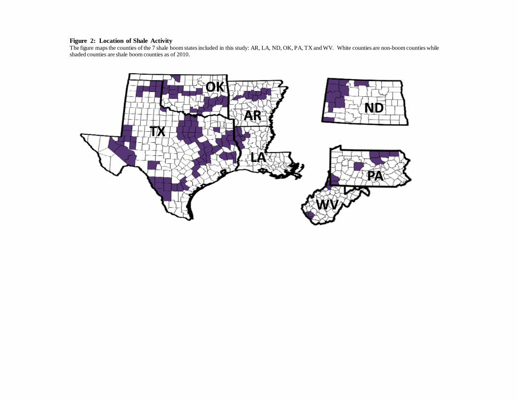
TX

OK

AR

LA

ND

WV

PA

Figure 2: Location of Shale ActivityThe figure maps the counties of the 7 shale boom states included in this study: AR, LA, ND, OK, PA, TX and WV. White counties are non-boom counties while shaded counties are shale boom counties as of 2010.

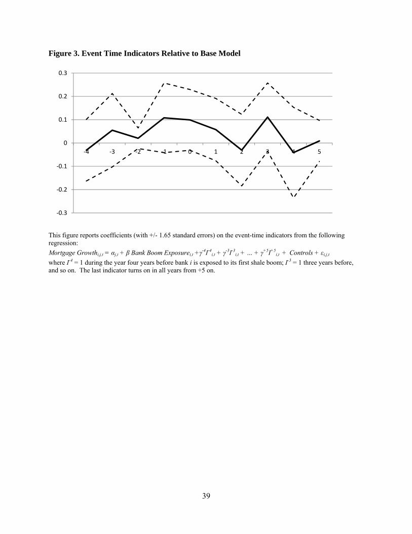
39

Figure 3. Event Time Indicators Relative to Base Model

This figure reports coefficients (with +/- 1.65 standard errors) on the event-time indicators from the following regression:

Mortgage Growthi,j,t = αj,t + β Bank Boom Exposurei,t +γ-4I-4

i,t + γ-3I-3i,t + … + γ+5I+5

i,t + Controls + εi,j,t

where I-4 = 1 during the year four years before bank i is exposed to its first shale boom; I-3 = 1 three years before, and so on. The last indicator turns on in all years from +5 on.

‐0.3

‐0.2

‐0.1

0

0.1

0.2

0.3

‐4 ‐3 ‐2 ‐1 0 1 2 3 4 5

0%

10%

20%

30%

40%

50%

60%

70%

80%

90%

2000 2001 2002 2003 2004 2005 2006 2007 2008 2009 2010

Per

cent

age

of L

oans

Sec

urit

ized

Securitization Rate of Distant Loans Securitization Rate of Local Loans

Figure 4: Securitization and Sold Rates, Local vs. Distant LoansThis figure plots the fraction of loans that are securitized or sold for local versus distant loans over the sample period in our study. A local loan is defined as a loan made in the same county in which a bank has a branch, while a distant loan is a loan made in a county by a lender that does not have a branch.

Mean Std. Deviation Mean Std. DeviationPanel A: Exposure to Deposit Shock (bank-year variation)Share of Branches in Boom Counties 0 0 0.45 0.39Growth in Shale Well Exposure 0 0 0.25 0.51Number of Bank-YearsNumber of Banks

Panel B: Bank Characteristics (bank-year variation)Deposit Growth 0.085 0.141 0.102 0.156Log of Assets 12.451 1.390 13.428 2.090Deposits / Assets 0.827 0.086 0.827 0.087Cost of Deposits 0.022 0.010 0.017 0.008Liquid Assets / Assets 0.273 0.148 0.225 0.132Capital / Assets 0.099 0.028 0.101 0.029C&I Loans / Asset 0.112 0.090 0.145 0.087Mortgage Loans / Assets 0.347 0.137 0.323 0.117Net Income / Assets 0.009 0.008 0.008 0.011Loan Commitments / Assets 0.109 0.140 0.134 0.182Letters of Credits / Assets 0.006 0.011 0.010 0.020

Panel C: Annual Mortgage Growth Rates (bank-year variation)Growth in Mortgage Originations 0.112 0.621 0.117 0.576Growth in Retained Mortgages 0.077 0.672 0.091 0.618Growth in Sold Mortgages 0.107 1.159 0.098 1.097

Panel C: Annual Mortgage Growth Rates (bank-county-year variation)Growth in Mortgage Originations 0.023 1.123 0.027 1.058Growth in Retained Mortgages 0.013 1.200 0.017 1.159Growth in Sold Mortgages 0.039 1.117 0.036 1.014

1,350 357

Table 1: Summary Statistics

Non-Exposed Banks Exposed Banks

7,451 1,280

This table reports summary statistics for banks operating in states with counties exposed to the shale boom. Theunit of observation is bank-year in Panel A and Panel B, and bank-county-year in Panel C. The sample is builtfrom the 7 states that experienced shale booms between 2000 and 2010. Share of Branches in Boom Countiesequals the fraction of a bank's branches located in shale-boom counties (variable set to 0 before the onset of ashale boom). Growth in Shale Well Exposure equals the weighted exposure to the growth in the number of shalewells where the fraction of a bank’s branches in boom counties serve as weights. The distribution of bankbranches comes from the FDIC Summary of Deposits , which we use to determine whether or not a branch (or thebank that owns it) is or is not exposed to the boom. Bank characteristics come from year-end Call Reports . Growth in mortgage originations comes from the annual HMDA data.

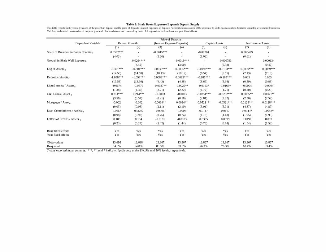
Dependent Variable(1) (2) (3) (4) (5) (6) (7) (8)

Share of Branches in Boom Countiest 0.0567*** - -0.0015*** - -0.00204 - 0.000479 -(4.03) - (2.66) - (1.08) - (0.61) -

Growth in Shale Well Exposuret - 0.0264*** - -0.0019*** - -0.000793 - 0.000134- (4.42) - (3.00) - (0.98) - (0.47)

Log of Assetst-1 -0.301*** -0.301*** 0.0036*** 0.0036*** -0.0193*** -0.0193*** 0.0039*** 0.0039***(14.56) (14.60) (10.13) (10.12) (6.54) (6.55) (7.13) (7.13)

Deposits / Assetst-1 -1.098*** -1.098*** 0.0083*** 0.0083*** -0.185*** -0.185*** 0.003 0.003(13.58) (13.60) (4.43) (4.38) (8.65) (8.64) (0.89) (0.88)

Liquid Assets / Assetst-1 -0.0674 -0.0679 -0.0027** -0.0029** -0.0163* -0.0163* -0.0004 -0.0004(1.38) (1.39) (2.21) (2.22) (1.72) (1.71) (0.20) (0.20)

C&I Loans / Assett-1 0.214*** 0.214*** -0.0003 -0.0003 -0.0251*** -0.0252*** 0.0065** 0.0065**(3.56) (3.57) (0.21) (0.18) (2.81) (2.82) (2.50) (2.52)

Mortgages / Assett-1 -0.002 -0.002 0.0034** 0.0034** -0.0521*** -0.0521*** 0.0128*** 0.0128***(0.03) (0.03) (2.11) (2.10) (5.01) (5.01) (4.87) (4.87)

Loan Commitments / Assetst-1 0.0667 0.0665 0.0006 0.0006 0.0117 0.0117 0.0043* 0.0043*(0.98) (0.98) (0.76) (0.74) (1.13) (1.13) (1.95) (1.95)

Letters of Credits / Assetst-1 0.103 0.104 -0.0101 -0.0103 0.0395 0.0399 0.0192 0.019(0.23) (0.24) (1.42) (1.44) (0.73) (0.74) (1.54) (1.53)

Bank fixed effects Yes Yes Yes Yes Yes Yes Yes YesYear fixed effects Yes Yes Yes Yes Yes Yes Yes Yes

Observations 13,698 13,698 13,867 13,867 13,867 13,867 13,867 13,867R-squared 54.8% 54.8% 89.5% 89.5% 76.3% 76.3% 63.4% 63.4%T-stats reported in parentheses. ***, **, and * indicate significance at the 1%, 5% and 10% levels, respectively.

Net Income/Assets

This table reports bank-year regressions of the growth in deposit and the price of deposits (interest expenses on deposits / deposits) on measures of the exposure to shale-boom counties. Controls variables are compiled based on Call Report data and measured as of the prior year end. Standard errors are clustered by bank. All regressions include bank and year fixed effects.

Table 2: Shale Boom Exposure Expands Deposit Supply

Deposit GrowthPrice of Deposits

(Interest Expense/Deposits) Capital/Assets

Dependent Variable(1) (2) (3) (4) (5) (6)

Share of Branches in Boom Countiest 0.146** - 0.325** - 0.202 -(2.17) - (2.26) - (1.26) -

Growth in Shale Well Exposuret - 0.0533** - 0.223*** - 0.0674- (1.97) - (2.69) - (1.37)

Log of Assetst-1 -0.0121 -0.0124 -0.0096 -0.0107 -0.0217** -0.0224**(1.45) (1.49) (1.11) (1.27) (2.10) (2.15)

Deposits / Assetst-1 (0.07) (0.07) (0.31) (0.29) 0.06 0.07(0.41) (0.39) (1.40) (1.32) (0.31) (0.33)

Cost of Depositst-1 (1.27) (1.31) (0.88) (0.96) (6.30) (6.43)(0.43) (0.44) (0.24) (0.27) (1.37) (1.39)

Liquid Assets / Assetst-1 0.151 0.144 -0.0596 -0.0864 0.497** 0.486**(1.08) (1.03) (0.31) (0.45) (2.58) (2.53)

Capital / Assetst-1 -1.442** -1.439** -0.243 -0.173 -1.987*** -1.990***(2.20) (2.20) (0.39) (0.28) (2.92) (2.94)

C&I Loans / Assett-1 0.081 0.0829 -0.0453 -0.0575 0.214 0.222(0.54) (0.55) (0.16) (0.20) (0.70) (0.73)

Mortgage Loans / Assetst-1 0.0445 0.031 -0.0104 -0.0697 0.289* 0.269(0.29) (0.20) (0.05) (0.33) (1.73) (1.54)

Net Income / Assetst-1 4.441** 4.517** 5.606* 5.764* 2.474 2.593(2.29) (2.33) (1.76) (1.78) (0.76) (0.80)

Loan Commitments / Assetst-1 0.0301 0.0292 -0.0191 -0.0222 0.0218 0.0194(1.32) (1.28) (0.51) (0.59) (0.57) (0.51)

Letters of Credits / Assetst-1 0.787 0.768 0.402 0.452 2.525** 2.497**(0.94) (0.92) (0.47) (0.53) (2.25) (2.23)

Borrower Controls Yes Yes Yes Yes Yes YesCounty*Year FE Yes Yes Yes Yes Yes YesBank Clustered St Errors Yes Yes Yes Yes Yes Yes

Observations 92,144 92,144 71,034 71,034 49,427 49,427R-squared 7.3% 7.3% 7.9% 8.0% 13.0% 13.0%T-stats are reported in parentheses. ***, **, and * indicate significance at the 1%, 5% and 10% levels, respectively.

Table 3: Effect of Liquidity Supply on Mortgage Lending

This table reports reduced form regressions of the percentage change in mortgage originations by bank-county-year on measures of the exposure toshale-boom counties. Bank-county-years are excluded if the county experienced a shale boom over the sample period. Mortgage Growth equals thepercentage change in originations from the prior year; Retained Growth equals the percentage change in mortgages held on the lender's balance sheet;Sold Growth equals the percentage change in mortgages sold by the originator. Regressions include both lender (reported) and borrower (notreported) control variables. Lender controls are from the Call Reports from the prior year; borrower controls are the average borrower and areaincome, loan size-to-income ratio, percent women applicants, percent of minority applicants, and percent minority in the area for loans made during thecurrent year (from HMDA). Standard errors are clustered by bank. All regressions also include county*year fixed effects.

Mortgage Growth Retained Growth Sold Growth

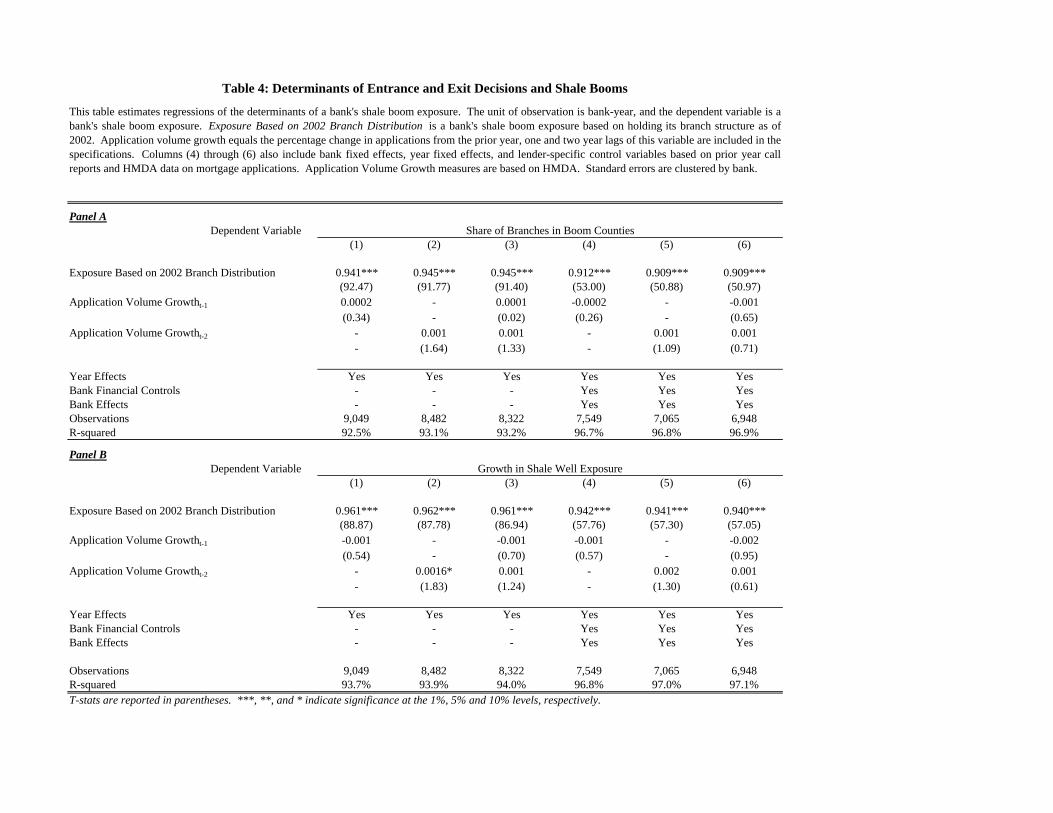
Panel ADependent Variable

(1) (2) (3) (4) (5) (6)

Exposure Based on 2002 Branch Distribution 0.941*** 0.945*** 0.945*** 0.912*** 0.909*** 0.909***(92.47) (91.77) (91.40) (53.00) (50.88) (50.97)

Application Volume Growtht-1 0.0002 - 0.0001 -0.0002 - -0.001(0.34) - (0.02) (0.26) - (0.65)

Application Volume Growtht-2 - 0.001 0.001 - 0.001 0.001- (1.64) (1.33) - (1.09) (0.71)

Year Effects Yes Yes Yes Yes Yes YesBank Financial Controls - - - Yes Yes YesBank Effects - - - Yes Yes YesObservations 9,049 8,482 8,322 7,549 7,065 6,948R-squared 92.5% 93.1% 93.2% 96.7% 96.8% 96.9%

Panel BDependent Variable

(1) (2) (3) (4) (5) (6)

Exposure Based on 2002 Branch Distribution 0.961*** 0.962*** 0.961*** 0.942*** 0.941*** 0.940***(88.87) (87.78) (86.94) (57.76) (57.30) (57.05)

Application Volume Growtht-1 -0.001 - -0.001 -0.001 - -0.002(0.54) - (0.70) (0.57) - (0.95)

Application Volume Growtht-2 - 0.0016* 0.001 - 0.002 0.001- (1.83) (1.24) - (1.30) (0.61)

Year Effects Yes Yes Yes Yes Yes YesBank Financial Controls - - - Yes Yes YesBank Effects - - - Yes Yes Yes

Observations 9,049 8,482 8,322 7,549 7,065 6,948R-squared 93.7% 93.9% 94.0% 96.8% 97.0% 97.1%T-stats are reported in parentheses. ***, **, and * indicate significance at the 1%, 5% and 10% levels, respectively.

Table 4: Determinants of Entrance and Exit Decisions and Shale Booms

This table estimates regressions of the determinants of a bank's shale boom exposure. The unit of observation is bank-year, and the dependent variable is abank's shale boom exposure. Exposure Based on 2002 Branch Distribution is a bank's shale boom exposure based on holding its branch structure as of2002. Application volume growth equals the percentage change in applications from the prior year, one and two year lags of this variable are included in the specifications. Columns (4) through (6) also include bank fixed effects, year fixed effects, and lender-specific control variables based on prior year callreports and HMDA data on mortgage applications. Application Volume Growth measures are based on HMDA. Standard errors are clustered by bank.

Share of Branches in Boom Counties

Growth in Shale Well Exposure

(1) (2) (3) (4) (5) (6) (7) (8) (9) (10) (11) (12)

Share of Branches in Boom Counties 0.177** - 0.148** 0.183** - 0.153** 0.230*** - 0.273*** -(2.18) - (2.20) (2.17) - (2.24) (3.22) - (5.89) -

Growth in Shale Well Exposure - 0.0535* 0.0566** - 0.061*** 0.0555* - 0.0616** - 0.110***- (1.87) (1.99) - (2.00) (1.91) - (2.32) - (6.55)

Pre-Boom Indicator for Booming Banks 0.014 0.014 - - - - - - - - - -(0.38) (0.36) - - - - - - - - - -

Growth in Branches - - 0.125* 0.126* - - - - - - - -- - (1.67) (1.67) - - - - - - - -

Borrower & Lender Controls Yes Yes Yes Yes Yes Yes Yes Yes Yes Yes Yes YesCounty*Year Fixed Effects Yes Yes Yes Yes Yes Yes Yes Yes Yes Yes Yes YesBank Clustered St Errors Yes Yes Yes Yes Yes Yes Yes Yes Yes Yes Yes YesBank*County Fixed Effects - - - - - - - - - - Yes Yes

Observations 92,144 92,144 92,144 92,144 62,189 62,189 90,926 90,926 30,365 30,365 92,144 92,144R-squared 7.3% 7.3% 7.4% 7.4% 7.0% 7.1% 7.4% 7.4% 19.7% 19.7% 16.5% 16.5%T-stats are reported in parentheses. ***, **, and * indicate significance at the 1%, 5% and 10% levels, respectively.

Bank-County observations with at Least

15 Mortgages

Drop Large, Nationwide Banks

Bank*County Fixed Effects

Table 5: Robustness Tests

This table estimates reduced form regressions of the percentage change in mortgage originations by bank-county-year using different robustness specifications. Bank-county-years are excluded if a county experienced a shale boom over the sample period. Mortgage Growth equals the percentage change in originations from the prior year. Regressions include both lender (not reported) and borrower (not reported) control variables. Lender controls are from the Call Reports from the prior year; borrower controls are from HMDA. Columns (1) and (2) report the analysis of parallel trends of exposed and non-exposed banks. The Pre-Boom Indicator for Booming Banks is equal to 1 for booming banks in all the years leading to the boom exposure and zero otherwise. The indicator is always equal to zero for banks that have never been exposed to the boom. Columns (3) and (4) add a control for branch growth. Columns (5) and (6) report results based on counties that do not border any of the boom counties. In columns (7) and (8) we eliminate banks with assets in the top decile of the size distribution. Columns (9) and (10) report results based on bank-county-years where lender originated at least 15 mortgages in two subsequent years. Finally, in columns (11) and (12) we incorporate bank*county fixed effects. All regressions include county-year fixed effects. Standard errors are clustered by bank.

Parallel Trend TestsExcluding Counties Neighboring Boom

Counties

Dependent Variable: Mortgage Growth

Include Branch Growth

Dependent Variable

(1) (2) (3) (4)

Local-Lender Indicator 0.009 0.010 - -(0.59) (0.67) - -

Share of Branches in Boom Counties 0.116 - 0.288*** -(1.36) - (2.94) -

Growth in Shale Well Exposure - 0.044 - 0.131**- (1.53) - (2.33)

Share of Branches in Boom Counties * 0.269** - - -Local-Lender Indicator (2.53) - - -

Growth in Shale Well Exposure - 0.146** - -Local-Lender Indicator - (2.16) - -

Log of Assetst-1 -0.012 -0.012 0.009 0.009(1.44) (1.47) (1.08) (1.10)

Deposits / Assetst-1 -0.080 -0.076 0.411*** 0.409***(0.46) (0.44) (3.97) (3.95)

Cost of Depositst-1 -1.183 -1.217 -1.481 -1.477(0.40) (0.41) (0.27) (0.27)

Liquid Assets / Assetst-1 0.149 0.143 0.271** 0.272**(1.06) (1.02) (2.25) (2.25)

Capital / Assetst-1 -1.462** -1.458** -0.323 -0.320(2.24) (2.23) (0.50) (0.49)

C&I Loans / Assett-1 0.081 0.083 0.200 0.206(0.54) (0.55) (1.25) (1.28)

Mortgage Loans / Assetst-1 0.052 0.039 0.064 0.061(0.34) (0.25) (0.40) (0.38)

Net Income / Assetst-1 4.410** 4.483** 2.013 2.075(2.28) (2.31) (0.79) (0.81)

Loan Commitments / Assetst-1 0.031 0.030 -0.106 -0.108(1.35) (1.31) (0.77) (0.78)

Letters of Credits / Assetst-1 0.801 0.778 -0.232 -0.281(0.95) (0.93) (0.33) (0.40)

Borrower Controls Yes Yes Yes YesCounty*Year FE Yes Yes Yes YesBank Clustered St Errors Yes Yes Yes Yes

Observations 92,144 92,144 22,192 22,192R-squared 7.3% 7.3% 20.2% 20.2%T-stats are reported in parentheses. ***, **, and * indicate significance at the 1%, 5% and 10% levels, respectively.

Table 6: Liquidity Supply and Mortgage Lending:The Effect of Local Lenders

This table reports reduced form regressions of the percentage change in mortgage originations by bank-county-year. Bank-county-yearsare excluded if the county actually a shale boom during the sample period. Local Lenders are those with a branch in the county (distantlenders originate mortgages without a branch in the county). Mortgage Growth equals the percentage change in originations from theprior year. Regressions include both lender (reported) and borrower (not reported) control variables. Lender controls are from the CallReports from the prior year; borrower controls are the average borrower and area income, loan size-to-income ratio, percent womenapplicants, percent of minority applicants, and percent minority in the area for loans made during the current year (from HMDA).Standard errors are clustered by bank. All regressions also include county*year fixed effects.

All Lenders Local Lenders OnlyMortgage Growth

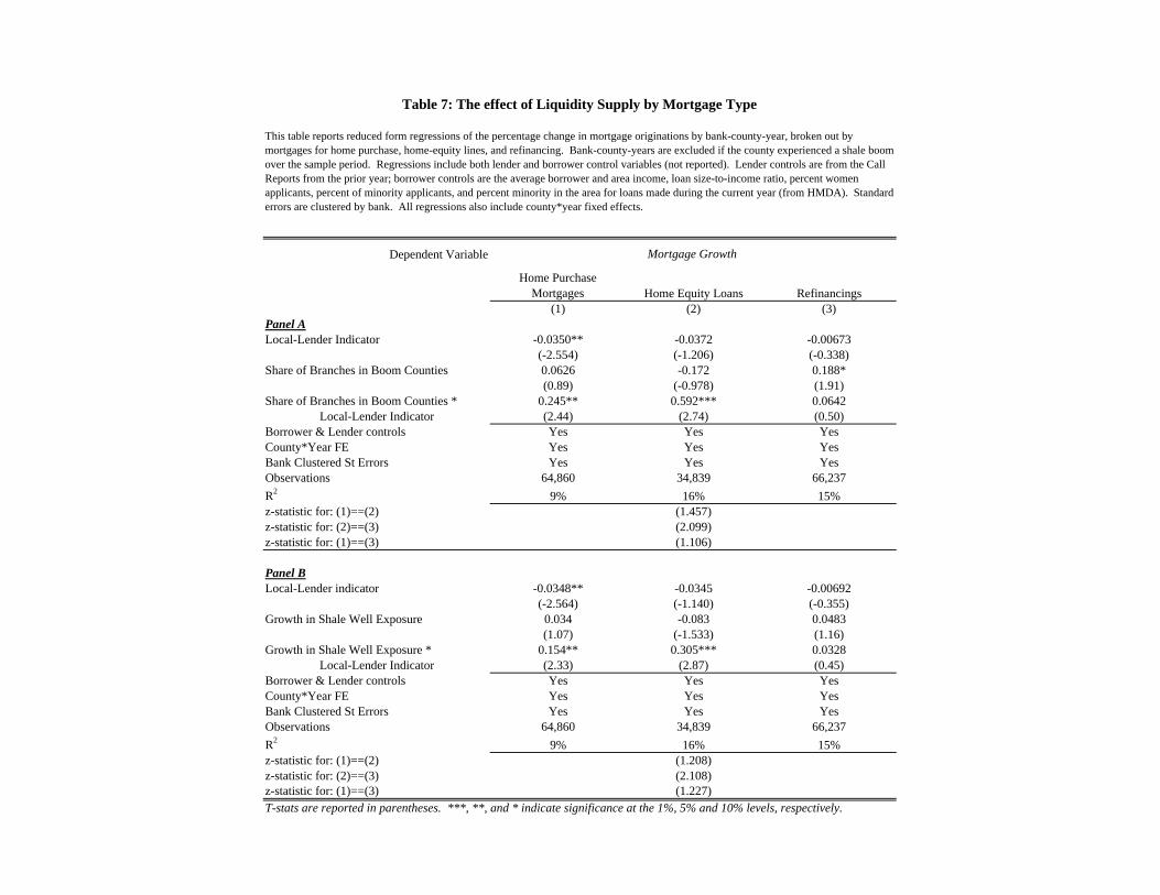
Dependent Variable

Home Purchase Mortgages Home Equity Loans Refinancings

(1) (2) (3)Panel ALocal-Lender Indicator -0.0350** -0.0372 -0.00673

(-2.554) (-1.206) (-0.338)Share of Branches in Boom Counties 0.0626 -0.172 0.188*

(0.89) (-0.978) (1.91)Share of Branches in Boom Counties * 0.245** 0.592*** 0.0642

Local-Lender Indicator (2.44) (2.74) (0.50)Borrower & Lender controls Yes Yes YesCounty*Year FE Yes Yes YesBank Clustered St Errors Yes Yes YesObservations 64,860 34,839 66,237R2 9% 16% 15%z-statistic for: (1)==(2)z-statistic for: (2)==(3)z-statistic for: (1)==(3)

Panel BLocal-Lender indicator -0.0348** -0.0345 -0.00692

(-2.564) (-1.140) (-0.355)Growth in Shale Well Exposure 0.034 -0.083 0.0483

(1.07) (-1.533) (1.16)Growth in Shale Well Exposure * 0.154** 0.305*** 0.0328

Local-Lender Indicator (2.33) (2.87) (0.45)Borrower & Lender controls Yes Yes YesCounty*Year FE Yes Yes YesBank Clustered St Errors Yes Yes YesObservations 64,860 34,839 66,237R2 9% 16% 15%z-statistic for: (1)==(2)z-statistic for: (2)==(3)z-statistic for: (1)==(3)T-stats are reported in parentheses. ***, **, and * indicate significance at the 1%, 5% and 10% levels, respectively.

(1.208)(2.108)(1.227)

Table 7: The effect of Liquidity Supply by Mortgage Type

This table reports reduced form regressions of the percentage change in mortgage originations by bank-county-year, broken out by mortgages for home purchase, home-equity lines, and refinancing. Bank-county-years are excluded if the county experienced a shale boom over the sample period. Regressions include both lender and borrower control variables (not reported). Lender controls are from the Call Reports from the prior year; borrower controls are the average borrower and area income, loan size-to-income ratio, percent women applicants, percent of minority applicants, and percent minority in the area for loans made during the current year (from HMDA). Standard errors are clustered by bank. All regressions also include county*year fixed effects.

Mortgage Growth

(1.457)(2.099)(1.106)

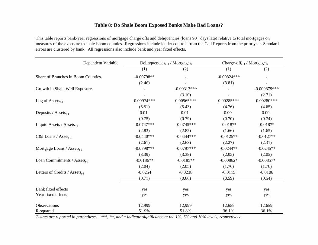
Dependent Variable(1) (2) (1) (2)

Share of Branches in Boom Countiest -0.00798** - -0.00324*** -(2.46) - (3.81) -

Growth in Shale Well Exposuret - -0.00313*** - -0.000879***- (3.10) - (2.71)

Log of Assetst-1 0.00974*** 0.00965*** 0.00285*** 0.00280***(5.51) (5.43) (4.76) (4.65)

Deposits / Assetst-1 0.01 0.01 0.00 0.00(0.75) (0.79) (0.70) (0.74)

Liquid Assets / Assetst-1 -0.0747*** -0.0745*** -0.0187* -0.0187*(2.83) (2.82) (1.66) (1.65)

C&I Loans / Assett-1 -0.0440*** -0.0444*** -0.0125** -0.0127**(2.61) (2.63) (2.27) (2.31)

Mortgage Loans / Assetst-1 -0.0798*** -0.0797*** -0.0244** -0.0245**(3.39) (3.38) (2.05) (2.05)

Loan Commitments / Assetst-1 -0.0186** -0.0185** -0.00862* -0.00857*(2.04) (2.05) (1.76) (1.76)

Letters of Credits / Assetst-1 -0.0254 -0.0238 -0.0115 -0.0106(0.71) (0.66) (0.59) (0.54)

Bank fixed effects yes yes yes yesYear fixed effects yes yes yes yes

Observations 12,999 12,999 12,659 12,659R-squared 51.9% 51.8% 36.1% 36.1%T-stats are reported in parentheses. ***, **, and * indicate significance at the 1%, 5% and 10% levels, respectively.

Delinquenciest+1 / Mortgagest Charge-offt+1 / Mortgagest

This table reports bank-year regressions of mortgage charge offs and deliquencies (loans 90+ days late) relative to total mortgages on measures of the exposure to shale-boom counties. Regressions include lender controls from the Call Reports from the prior year. Standard errors are clustered by bank. All regressions also include bank and year fixed effects.

Table 8: Do Shale Boom Exposed Banks Make Bad Loans?

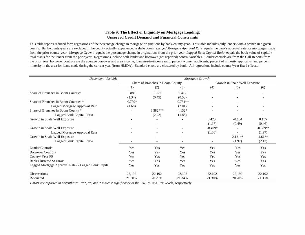
Dependent Variable

(1) (2) (3) (4) (5) (6)Share of Branches in Boom Counties 0.888 -0.176 0.417 - - -

(1.34) (0.45) (0.58) - - -Share of Branches in Boom Counties * -0.799* -0.731** - - -

Lagged Mortgage Approval Rate (1.68) (2.01) - - -Share of Branches in Boom County * - 3.582*** 4.132* - - -

Lagged Bank Capital Ratio - (2.92) (1.85) - - -Growth in Shale Well Exposure - - - 0.423 -0.104 0.155

- - - (1.17) (0.49) (0.46)Growth in Shale Well Exposure - - - -0.409* - -0.389**

Lagged Mortgage Approval Rate - - - (1.86) - (1.97)Growth in Shale Well Exposure - - - - 2.131** 4.61**

Lagged Bank Capital Ratio - - - - (1.97) (2.13)

Lender Controls Yes Yes Yes Yes Yes YesBorrower Controls Yes Yes Yes Yes Yes YesCounty*Year FE Yes Yes Yes Yes Yes YesBank Clustered St Errors Yes Yes Yes Yes Yes YesLagged Mortgage Approval Rate & Lagged Bank Capital Yes Yes Yes Yes Yes Yes

Observations 22,192 22,192 22,192 22,192 22,192 22,192R-squared 21.30% 20.20% 21.34% 21.30% 20.20% 21.35%T-stats are reported in parentheses. ***, **, and * indicate significance at the 1%, 5% and 10% levels, respectively.

Table 9: The Effect of Liquidity on Mortgage Lending:Unserved Credit Demand and Financial Constraints

This table reports reduced form regressions of the percentage change in mortgage originations by bank-county-year. This table includes only lenders with a branch in a given county. Bank-county-years are excluded if the county actually experienced a shale boom. Lagged Mortgage Approval Rate equals the bank's approval rate for mortgages made from the prior county-year. Mortgage Growth equals the percentage change in originations from the prior year; Lagged Bank Capital Ratio equals the book value of capital / total assets for the lender from the prior year. Regressions include both lender and borrower (not reported) control variables. Lender controls are from the Call Reports from the prior year; borrower controls are the average borrower and area income, loan size-to-income ratio, percent women applicants, percent of minority applicants, and percent minority in the area for loans made during the current year (from HMDA). Standard errors are clustered by bank. All regressions include county*year fixed effects.

Mortgage GrowthShare of Branches in Boom County Growth in Shale Well Exposure

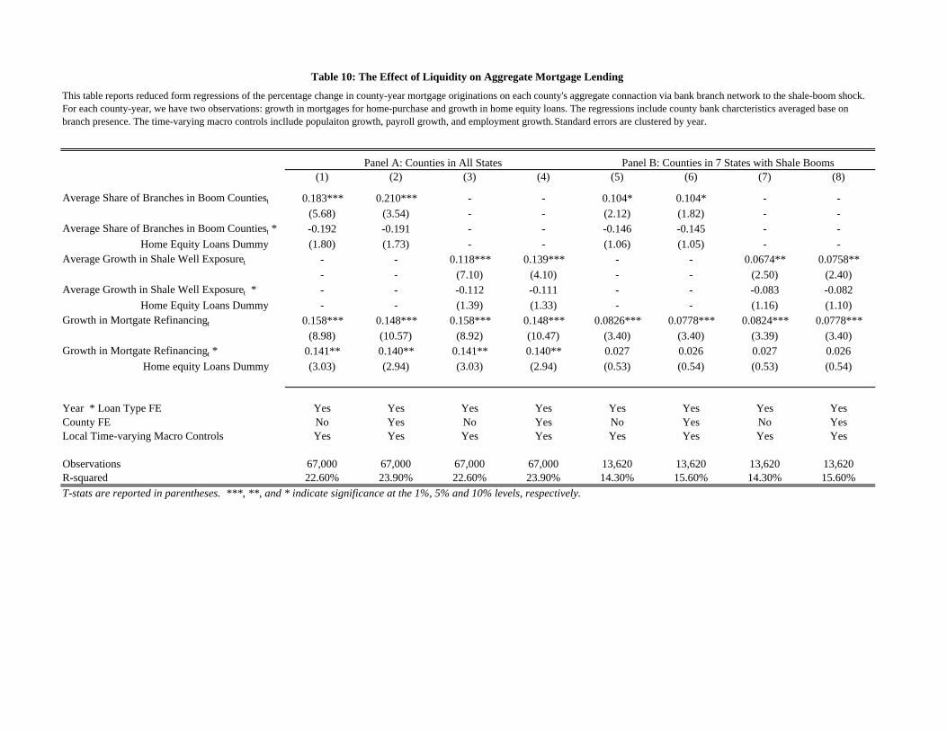
(1) (2) (3) (4) (5) (6) (7) (8)

Average Share of Branches in Boom Countiest 0.183*** 0.210*** - - 0.104* 0.104* - -(5.68) (3.54) - - (2.12) (1.82) - -

Average Share of Branches in Boom Countiest * -0.192 -0.191 - - -0.146 -0.145 - - Home Equity Loans Dummy (1.80) (1.73) - - (1.06) (1.05) - -

Average Growth in Shale Well Exposuret - - 0.118*** 0.139*** - - 0.0674** 0.0758**- - (7.10) (4.10) - - (2.50) (2.40)

Average Growth in Shale Well Exposuret * - - -0.112 -0.111 - - -0.083 -0.082 Home Equity Loans Dummy - - (1.39) (1.33) - - (1.16) (1.10)

Growth in Mortgate Refinancingt 0.158*** 0.148*** 0.158*** 0.148*** 0.0826*** 0.0778*** 0.0824*** 0.0778***(8.98) (10.57) (8.92) (10.47) (3.40) (3.40) (3.39) (3.40)

Growth in Mortgate Refinancingt * 0.141** 0.140** 0.141** 0.140** 0.027 0.026 0.027 0.026 Home equity Loans Dummy (3.03) (2.94) (3.03) (2.94) (0.53) (0.54) (0.53) (0.54)

Year * Loan Type FE Yes Yes Yes Yes Yes Yes Yes YesCounty FE No Yes No Yes No Yes No YesLocal Time-varying Macro Controls Yes Yes Yes Yes Yes Yes Yes Yes

Observations 67,000 67,000 67,000 67,000 13,620 13,620 13,620 13,620R-squared 22.60% 23.90% 22.60% 23.90% 14.30% 15.60% 14.30% 15.60%T-stats are reported in parentheses. ***, **, and * indicate significance at the 1%, 5% and 10% levels, respectively.

Table 10: The Effect of Liquidity on Aggregate Mortgage Lending

This table reports reduced form regressions of the percentage change in county-year mortgage originations on each county's aggregate connaction via bank branch network to the shale-boom shock. For each county-year, we have two observations: growth in mortgages for home-purchase and growth in home equity loans. The regressions include county bank charcteristics averaged base on branch presence. The time-varying macro controls incllude populaiton growth, payroll growth, and employment growth. Standard errors are clustered by year.

Panel A: Counties in All States Panel B: Counties in 7 States with Shale Booms