EXPORT PRICE VOLATILITY OF REFINED PETROLEUM PRODUCTS FROM A SMALL HYDROCARBON BASED ECONOMYRoger Hosein, Don Charles, Martin Franklin

1

EXPORT PRICE VOLATILITY OF REFINED PETROLEUM PRODUCTS FROM A SMALL HYDROCARBON BASED

ECONOMY

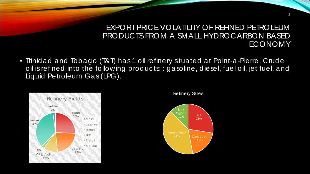
• Trinidad and Tobago (T&T) has 1 oil refinery situated at Point-a-Pierre. Crude oil is refined into the following products: : gasoline, diesel, fuel oil, jet fuel, and Liquid Petroleum Gas (LPG).

diesel26%

gasoline23%

jetfuel12%

LPG2%

fuel oil35%

fuel loss2%

Refinery Yields

diesel

gasoline

jetfuel

LPG

fuel oil

fuel loss

T&T 28%

Caribbean19%

International41%

Extra Regional

12%

Refinery Sales

2

EXPORT PRICE VOLATILITY OF REFINED PETROLEUM PRODUCTS FROM A SMALL HYDROCARBON BASED

ECONOMY

• The Gross margin is the weighted average price of refinery fractions less the price of crude oil. Within the recent years, the refinery margins have began to decline. This has negatively impacted the profitability of Petrotrin’srefinery.

-$0.20

-$0.10

$0.00

$0.10

$0.20

$0.30

$0.40

$0.50

$0.60

$0.70

$0.80

1986

1988

1990

1992

1994

1996

1998

2000

2002

2004

2006

2008

2010

2012

US $

per

gal

lon

Gross Margin

Gross Margin

The profitability of the refinery is of interest to T&T because: provide employment for 5,000 persons, sources services from 2,000 registered contractors, maintain roads and bridges that connects to its operations, and implements a number of positive externality projects

3

EXPORT PRICE VOLATILITY OF REFINED PETROLEUM PRODUCTS FROM A SMALL HYDROCARBON BASED

ECONOMY

• Since refinery margins are influenced by the prices of the refinery fractions this study seeks to model the volatility of refinery fraction prices.

• Crude oil prices and refinery fraction prices are volatile. Volatility is the tendency of a series to fluctuate.

• Volatility is a also measure of risk. It is the tendency for the price of a commodity to deviate from its mean price. We are concerned about volatility because it measures the tendency of the price of refinery fractions to decline and thus refinery margins would get smaller.

4

EXPORT PRICE VOLATILITY OF REFINED PETROLEUM PRODUCTS FROM A SMALL HYDROCARBON BASED

ECONOMY

• Objective: This study seeks to study the volatility of prices of the following commodities: gasoline, diesel, heating oil, and jet fuel. This study is distinguished from other studies by:

• The length of the study and the utilization of the most recent data;• The utilization of both real and nominal data, as previous research neglected

real data;• The consideration of a pre & post financial crisis (US Shale boom era);• Including oil prices in the mean equation;• Testing for volatility spillover for diesel, gasoline, heating oil and jet fuel; • Implications of volatility for a small country refinery

5

DATA

• Source of data: • Both nominal and real data on the energy commodities are collected from

the US Energy Information Administration (EIA). Weekly nominal data is collected from 19th April, 1996 to 1st August, 2014. Such period is used because data was available for all variables within such period. Weekly data is used over annual data since it will produce 955 observations per variable.

• Real data is collected over the period January 1979 to August 2014. The monthly data generates 428 observations per variable. Weekly data was preferred but an appropriate deflator could not be found for weekly data.

6

METHODOLOGY

7

METHODOLOGY

Model EquationARCH (1)

GARCH (1, 1)

TARCH (1, 1)

EGARCH (1, 1)

The EGARCH model was used to test for asymmetric effects. The sign (leverage) effect is if negative shocks increase volatility more than positive shocks. The size effect is if large shocks increase volatility more than small shocks.

8

DIAGNOSTIC TESTS

As U tends to zero, the better the predictive accuracy, and as U tends to 1, the more unreliable the predictive accuracy

The smaller the value of the MSE and the MAE, the better the predictive accuracy

9

RESULTSACF Diesel PACF Diesel ACF gasoline PACF gasoline ACF WTI PACF WTI

|******* |******* |******* |******* |******* |*******|******* **| | |******* *| | |******* *| ||******* |* | |******* | | |******* | ||******* | | |******* *| | |******* | ||******* | | |******* | | |******* | ||******* | | |******* | | |******* | ||******* | | |******* | | |******* | ||******* | | |******* | | |******* | ||******* | | |******* | | |******* | ||******* | | |******* | | |******* | |

ACF heating oil PACF heating oil ACF jet fuel PACF jet fuel ACF propanePACF

propane

|******* |******* |******* |******* |******* |*******|******* *| | |******* *| | |******* *| ||******* |* | |******* | | |******* | ||******* | | |******* | | |******* | ||******* | | |******* | | |******* | ||******* | | |******* | | |******* | ||******* | | |******* | | |******* | ||******* | | |******* | | |******* | ||******* | | |******* | | |******* | ||******* | | |******* | | |******* | |

Table 1 A: ACF results at level

ACF D(diesel)PACF

D(diesel)ACF

D(gasoline)PACFD(gas

oline) ACF D(WTI) PACF D(WTI)

|** | |** | |* | |* | |* | |* |

| | *| | | | | | *| | *| |

| | | | |* | |* | |* | |* |

| | | | | | | | | | | |

| | | | | | | | | | | |

*| | *| | | | | | | | | |

*| | | | *| | *| | | | | |

| | | | | | | | |* | |* |

| | | | *| | *| | |* | | |

| | | | | | | | | | | |

ACF D(heating oil)

PACF D(heating

oil)ACF D(jet

fuel)PACF D(jet

fuel)ACF

D(propane) PACF D(propane)

|** | |** | |* | |* | |* | |* |

*| | *| | | | *| | | | | |

| | | | | | | | |* | |* |

| | | | | | | | |* | |* |

| | | | | | | | | | *| |

| | | | | | | | *| | | |

| | *| | | | | | | | | |

| | | | | | |* | | | | |

| | | | | | | | | | | |

| | | | | | |* | | | | |

Table 1 B: 1st

difference ACF results

All variables are non-stationary and I(1)

10

RESULTSNominal data Weekly from 19th April 1996 to 1st August 2014Variable ADF level ADF 1st Diff PP Level PP 1st diff KPS level KPS 1st diffLn gasoline 0.4876 0.0000 0.6184 0.0000 3.527408 0.031156Ln diesel 0.7088 0.0000 0.7172 0.0000 3.467929 0.058297Ln heat oil 0.7562 0.0000 0.7957 0.0000 3.529947 0.053852Ln jet fuel 0.6850 0.0000 0.7288 0.0000 3.519684 0.047815Ln lpg 0.3751 0.0000 0.3945 0.0000 3.004895 0.047909Ln WTI 0.7026 0.0000 0.7753 0.0000 3.540030 0.053420Real data Monthly from January 1979 to August 2014Ln gasoline 0.3826 0.0000 0.5671 0.0000 0.683519 0.144884Ln diesel 0.3010 0.0000 0.3722 0.0000 0.587386 0.118427Ln heat oil 0.4860 0.0000 0.6271 0.0000 0.802313 0.136739Ln WTI 0.2331 0.0000 0.4471 0.0000 0.673827 0.112796

Table 3: Stationary results

All variables are I(1)

Source: Computed

11

RESULTSVariable Nominal data

resultsReal data results Variable Nominal data results Real data

resultsGasolinereturns

JB 485.83

prob. 0.0000

Kurtosis 6.49

Skewness -0.01

JB 1019.74

prob. 0.0000

Kurtosis 10.28

Skewness -1.02

Heatingoil returns

JB 2767.24

prob. 0.0000

Kurtosis 11.33

Skewness 0.13

JB 1526.62

prob. 0.0000

Kurtosis 12.09

Skewness 0.88Dieselreturns

JB 307.68

prob. 0.0000

Kurtosis 5.76

Skewness 0.17

JB 183.05

prob. 0.0000

Kurtosis 6.11

Skewness -0.39

Propanereturns

JB 4991.09

prob. 0.0000

Kurtosis 14.18

Skewness -0.34Jet fuelreturns

JB 220.7

prob. 0.0000

Kurtosis 5.33

Skewness -0.14

WTIreturns

JB 402.65

prob. 0.0000

Kurtosis 6.12

Skewness -0.31

JB 379.21

prob. 0.0000

Kurtosis 7.45

Skewness -0.61

Table 4: Normality results

Source: Computed

Low JB probabilities result in the rejection of the null hypothesis that the series are normally distributed. Thus all variables are not Gaussian distributed. Thus ARCH type modeling is appropriate.

12

RESULTS

Variable Test Statistic Nominal data Real dataDiesel returns Prob. F(7,939) 0.0000 0.0001

Prob. Chi-Square(7) 0.0000 0.0001Log gasoline Prob. F(7,939) 0.0000 0.0000

Prob. Chi-Square(7) 0.0000 0.0000Log jet fuel Prob. F(7,939) 0.0000

Prob. Chi-Square(7) 0.0000Log heating oil Prob. F(7,939) 0.0002 0.0000

Prob. Chi-Square(7) 0.0002 0.0000Log propane Prob. F(7,939) 0.0000

Prob. Chi-Square(7) 0.0000Log WTI Prob. F(7,939) 0.0000 0.0000

Prob. Chi-Square(7) 0.0000 0.0000

Table 5: ARCH effects results

Low probabilities result in the rejection of the null of no ARCH effects are present. Thus GARCH type modeling is appropriate.

13

RESULTSGARCH Nominal diesel Coefficient Std. Error z-Statistic Prob.

Mean Eq. RW 0.7028 0.0200 35.1294 0.0000Variance Eq. C 0.0000 0.0000 2.5014 0.0124

ARCH(-1) 0.2054 0.0407 5.0502 0.0000GARCH(-1) 0.7991 0.0292 27.3702 0.0000

EGARCH Nominal diesel Coefficient Std. Error z-Statistic Prob.Mean Eq. RW 0.7051 0.0186 37.8089 0.0000Variance Eq. C(2) constant -0.5589 0.1113 -5.0192 0.0000

C(3) size effect 0.3718 0.0542 6.8631 0.0000C(4) leverage effect 0.0834 0.0335 2.4880 0.0128

C(5) GARCH term 0.9589 0.0137 69.9322 0.0000

GARCH Nominal gasoline Coefficient Std. Error z-Statistic Prob.Mean Eq. RW 0.8378 0.0238 35.1395 0.0000Variance Eq. C 0.0001 0.0000 3.2345 0.0012

ARCH(-1) 0.2372 0.0460 5.1549 0.0000GARCH(-1) 0.7094 0.0464 15.2734 0.0000

EGARCH Nominal gasoline Coefficient Std. Error z-Statistic Prob.Mean Eq. RW 0.8569 0.0227 37.8288 0.0000Variance Eq. C(2) constant -0.7742 0.1734 -4.4636 0.0000

C(3) size effect 0.3393 0.0568 5.9707 0.0000C(4) leverage effect 0.1320 0.0363 3.6342 0.0003

C(5) GARCH term 0.9240 0.0227 40.7086 0.0000

GARCH Nominal heat oil Coefficient Std. Error z-Statistic Prob.Mean Eq. RW 0.8113 0.0153 52.9572 0.0000

Variance Eq. C 0.0001 0.0000 3.7531 0.0002ARCH(-1) 0.1977 0.0401 4.9355 0.0000

GARCH(-1) 0.7309 0.0410 17.8254 0.0000EGARCH Nominal heat oil Coefficient Std. Error z-Statistic Prob.Mean Eq. RW 0.8184 0.0150 54.6137 0.0000

Variance Eq. C(2) constant -0.7667 0.1678 -4.5697 0.0000C(3) size effect 0.3329 0.0512 6.5008 0.0000

C(4) leverage effect 0.0717 0.0343 2.0929 0.0364C(5) GARCH term 0.9319 0.0196 47.5188 0.0000

GARCH Nominal jet fuel Coefficient Std. Error z-Statistic Prob.Mean Eq. RW 0.7837 0.0173 45.3244 0.0000

Variance Eq. C 0.0000 0.0000 3.4583 0.0005ARCH(-1) 0.2249 0.0431 5.2190 0.0000

GARCH(-1) 0.7328 0.0350 20.9512 0.0000EGARCH Nominal jet fuel Coefficient Std. Error z-Statistic Prob.Mean Eq. RW 0.7835 0.0170 46.1252 0.0000

Variance Eq. C(2) constant -0.8047 0.1633 -4.9290 0.0000C(3) size effect 0.3892 0.0554 7.0297 0.0000

C(4) leverage effect 0.0490 0.0365 1.3446 0.1788C(5) GARCH term 0.9295 0.0201 46.3412 0.0000

In all models, WTI is significant in the mean equation, suggesting oil prices affect refinery fraction prices.

14Table 6: GARCH and EGARCH results

The leverage effect for gasoline, diesel and heating oil were positive and significant. Thus negative shocks increase their volatility more than positive shocks. The leverage effect for jet fuel was insignificant, suggesting symmetric in sign of shock effects. For all models the GARCH term is large and over 0.71 suggesting the persistence of shocks.

DIAGNOSTIC TESTS

•

15

-.2

-.1

.0

.1

.2

.3

-.2 -.1 .0 .1 .2

Quantiles of RESIDUALDIESEL

Qua

ntile

s of

RES

IDU

ALW

TI

-.2

-.1

.0

.1

.2

.3

-.3 -.2 -.1 .0 .1 .2 .3 .4

Quantiles of RESIDUALGASOLINE

Qua

ntile

s of

RES

IDU

ALW

TI

Nominal data QQ plot of diesel residuals

QQ plot of gasoline residuals

WTI

resid

uals

Diesel residuals Gasoline residuals

WTI

resid

uals

The QQ plot shows how the distribution of 1 series matches the distribution of another series.

For all series, the refinery fraction residuals matched WTI residuals, however, positive and negative shocks caused the occasional deviation of a few data points

-.2

-.1

.0

.1

.2

.3

-.4 -.3 -.2 -.1 .0 .1 .2 .3

Quantiles of RESIDUALHOIL

Qua

ntile

s of

RES

IDU

ALW

TIW

TI re

sidua

ls

Heating oil residuals

RESULTSEquation Probability Equation ProbabilityDiesel-gasoline 0.0279 Gasoline-Diesel 0.0249Diesel-heating oil 0.0000 Gasoline-heating oil 0.0048Diesel-jet fuel 0.0000 Gasoline-jet fuel 0.0000Diesel-WTI 0.0025 Gasoline-WTI 0.0767Heating oil–diesel 0.0000 Jet fuel-Diesel 0.0000Heating oil-gasoline 0.0113 Jet fuel-gasoline 0.0000Heating oil-jet fuel 0.0000 Jet fuel-heating oil 0.0000Heating oil-WTI 0.0001 Jet fuel-WTI 0.0023

16

For each series, the variance term was significant in the volatility spill over equation. This suggested volatility spillover effects.E.g. It means that the volatility of diesel prices affects the volatility of gasoline prices.

Table 7: Volatility spillover effects.

DIAGNOSTIC RESULTSNominal data diesel gasoline Heating oil Jet fuelGARCH (1,1) MSE: 0.0393

MAE: 0.0272

Thiel: 0.5156

MSE: 0.0418

MAE: 0.0282

Thiel: 0.4679

MSE: 0.0316

MAE: 0.0192

Thiel: 0.4024

MSE: 0.0315

MAE: 0.0204

Thiel: 0.4109TARCH (1,1) MSE: 0.0393

MAE: 0.0272

Thiel: 0.5152

MSE: 0.0418

MAE: 0.0282

Thiel: 0.4656

MSE: 0.0316

MAE: 0.0192

Thiel: 0.4021

MSE: 0.0315

MAE: 0.0204

Thiel: 0.4104EGARCH(1,1) MSE: 0.0393

MAE: 0.0272

Thiel: 0.5151

MSE: 0.0418

MAE: 0.0282

Thiel: 0.4642

MSE: 0.0316

MAE: 0.0192

Thiel: 0.4014

MSE: 0.0315

MAE: 0.0204

Thiel: 0.4109Real dataGARCH (1,1) MSE: 0.0403

MAE: 0.0289

Thiel: 0.2638

MSE: 0.0369

MAE: 0.0265

Thiel: 0.4957

MSE: 0.0390

MAE: 0.0248

Thiel: 0.6615TARCH (1,1) MSE: 0.0403

MAE: 0.0289

Thiel: 0.2639

MSE: 0.0369

MAE: 0.0265

Thiel: 0.4951

MSE: 0.0390

MAE: 0.0248

Thiel: 0.6615EGARCH(1,1) MSE: 0.0403

MAE: 0.0289

Thiel: 0.2638

MSE: 0.0369

MAE: 0.0265

Thiel: 0.4902

MSE: 0.0388

MAE: 0.0246

Thiel: 0.6381

17

Low values of the MSE and the MAE suggested relatively good predictive accuracy

POLICY RECOMMENDATIONS

• In summary, gasoline, diesel, heating oil and jet fuel were all I(1). Their normality test results indicated that each series was not normally distributed. ARCH effects test results all indicated a presence of ARCH effects, thus GARCH type models were appropriate for modeling.

• There was volatility spillover between all series. This suggests that each refinery fraction’s volatility is affected by the volatility of the other refinery fractions. Given that refinery margins may be slim in the future, refiners need to take a number of steps to ensure their survival.

18

POLICY RECOMMENDATIONS

• A key factor to ensure the survival of refineries outside of the US is the controlling of costs. Such refineries need to cut their operational costs and find more to do with less. Refinery firms may redesign their core processes and automation, try to minimize shut in productions, better organization of shifts for workers, and concentrating on work that drives performance.

• The local refinery should try to increase oil production and use more locally produced crude as this will decrease refinery costs.

• The refinery firm can consider hedging with forwards contracts for both crude oil and refinery fractions. This is where they enter a contract today to pay an agreed price of oil, or get an agreed price of refinery products, but the delivery of the commodity will be at a future date.

19

CONCLUSION

• Thank you

20