Exponential Resolution Lower Bounds for Weak Pigeonhole

Exponential Resolution Lower Bounds for Weak PigeonholePrinciple and Perfect Matching Formulas over Sparse Graphs

Susanna F. de Rezende1, Jakob Nordstrom2,1, Kilian Risse1, and Dmitry Sokolov3,2

1KTH Royal Institute of Technology2University of Copenhagen

3Lund University

December 2, 2019

Abstract

We show exponential lower bounds on resolution proof length for pigeonhole principle (PHP)formulas and perfect matching formulas over highly unbalanced, sparse expander graphs, thus answer-ing the challenge to establish strong lower bounds in the regime between balanced constant-degreeexpanders as in [Ben-Sasson and Wigderson ’01] and highly unbalanced, dense graphs as in [Raz ’04]and [Razborov ’03, ’04]. We obtain our results by revisiting Razborov’s pseudo-width method forPHP formulas over dense graphs and extending it to sparse graphs. This further demonstrates thepower of the pseudo-width method, and we believe it could potentially be useful for attacking alsoother longstanding open problems for resolution and other proof systems.

1 Introduction

In one sentence, proof complexity is the study of efficient certificates of unsatisfiability for formulas inconjunctive normal form (CNF). In its most general form, this is the question of whether coNP can beseparated from NP or not, and as such appears out of reach for current techniques. However, if one insteadfocuses on concrete proof systems, which can be thought of as restricted models of nondeterministiccomputation, this opens up the view to a rich landscape of results.

One line of research in proof complexity has been to prove superpolynomial lower bounds for strongerand stronger proof systems, as a way of approaching the distant goal of establishing NP 6= coNP. Aperhaps even more fruitful direction, however, has been to study different combinatorial principles andinvestigate what kind of reasoning is needed to efficiently establish the validity of these principles. In thisway, one can quantify the “depth” of different mathematical truths, measured in terms of how strong aproof system is required to prove them.

In this paper, we consider the proof system resolution [Bla37], in which one derives new disjunctiveclauses from the formula until an explicit contradiction is reached. This is arguably the most well-studiedproof system in proof complexity, for which numerous exponential lower bounds on proof size havebeen shown (starting with [Hak85, Urq87, CS88]). Yet many basic questions about resolution remainstubbornly open. One such set of questions concerns the pigeonhole principle (PHP) stating that there isno injective mapping of m pigeons into n holes if m > n. This is one of the simplest, and yet most useful,combinatorial principles in mathematics, and it has been topic of extensive study in proof complexity.

When studying the pigeonhole principle, it is convenient to think of it in terms of a bipartite graphG = (U

.∪ V,E) with pigeons U = [m] and holes V = [n] for m ≥ n + 1. Every pigeon i can fly to

its neighbouring pigeonholes N(i) as specified by G, which for now we fix to be the complete bipartitegraph Km,n with N(i) = [n] for all i ∈ [m]. Since we wish to study unsatisfiable formulas, we encode the

ISSN 1433-8092

Electronic Colloquium on Computational Complexity, Report No. 174 (2019)

WEAK PIGEONHOLE PRINCIPLE AND PERFECT MATCHING OVER SPARSE GRAPHS

claim that there does in fact exist an injective mapping of pigeons to holes as a CNF formula consisting ofpigeon axioms

P i =∨

j∈N(i)

xij for i ∈ [m] (1.1a)

and hole axiomsH i,i′

j = (xij ∨ xi′j) for i 6= i′ ∈ [m], j ∈ N(i) ∩N(i′) (1.1b)

(where the intended meaning of the variables is that xi,j is true if pigeon i flies to hole j). To rule outmulti-valued mappings one can also add functionality axioms

F ij,j′ = (xij ∨ xij′) for i ∈ [m], j 6= j′ ∈ N(i) , (1.1c)

and a further restriction is to include surjectivity or onto axioms

Sj =∨

i∈N(j)

xij for j ∈ [n] (1.1d)

requiring that every hole should get a pigeon. Clearly, the “basic” pigeonhole principle (PHP) formulaswith clauses (1.1a) and (1.1b) are the least constrained. As one adds clauses (1.1c) to obtain the functionalpigeonhole principle (FPHP) and also clauses (1.1d) to get the onto functional pigeonhole principle (onto-FPHP), the formulas become more overconstrained and thus (potentially) easier to disprove, meaning thatestablishing lower bounds becomes harder. A moment of reflection reveals that onto-FPHP formulas arejust saying that complete bipartite graphs with m left vertices and n right vertices have perfect matchings,and so these formulas are also referred to as perfect matching formulas.

Another way of varying the hardness of PHP formulas is by letting the number of pigeons m growlarger as a function of the number of holes n. What this means is that it is not necessary to count exactlyto refute the formulas. Instead, it is sufficient to provide a precise enough estimate to show that m > nmust hold (where the hardness of this task depends on how much larger m is than n). Studying thehardness of such so-called weak PHP formulas gives a way of measuring how good different proofsystems are at approximate counting. A second application of lower bounds for weak PHP formulasis that they can be used to show that proof systems cannot produce efficient proofs of the claim thatNP * P/poly [Raz98, Raz04b].

Yet another version of more constrained formulas is obtained by restricting what choices the pigeonshave for flying into holes, by defining the formulas not overKm,n but sparse bipartite graphs with boundedleft degree—such instances are usually called graph PHP formulas. Again, this makes the formulaseasier to disprove in the sense that pigeons are more constrained, and it also removes the symmetry in theformulas that plays an essential role in many lower bound proofs.

Our work focuses on the most challenging setting in terms of lower bounds, when all of these restrictionsapply: the PHP formulas contain both functionality and onto axioms, the number of pigeonsm is very largecompared to the number of holes n, and the choices of holes are restricted by a sparse graph. But beforediscussing our contributions, let us review what has been known about resolution and pigeonhole principleformulas. We emphasize that what will follow is a brief and selective overview focusing on resolutiononly—see Razborov’s beautiful survey paper [Raz02] for a discussion of upper and lower bounds on PHPformulas in other proof systems.

1.1 Previous Work

In a breakthrough result, which served as a strong impetus for further developments in proof complexity,Haken [Hak85] proved a lower bound exp(Ω(n)) on resolution proof length for m = n + 1 pigeons.Haken’s proof was for the basic PHP formulas, but easily extends to onto-FPHP formulas. This result wassimplified and improved in a sequence of works [BT88, BP96, BW01, Urq03] to a lower bound of theform exp

(n2/m

), which, unfortunately, does not yield anything nontrivial for m = Ω

(n2)

pigeons.

2

1 Introduction

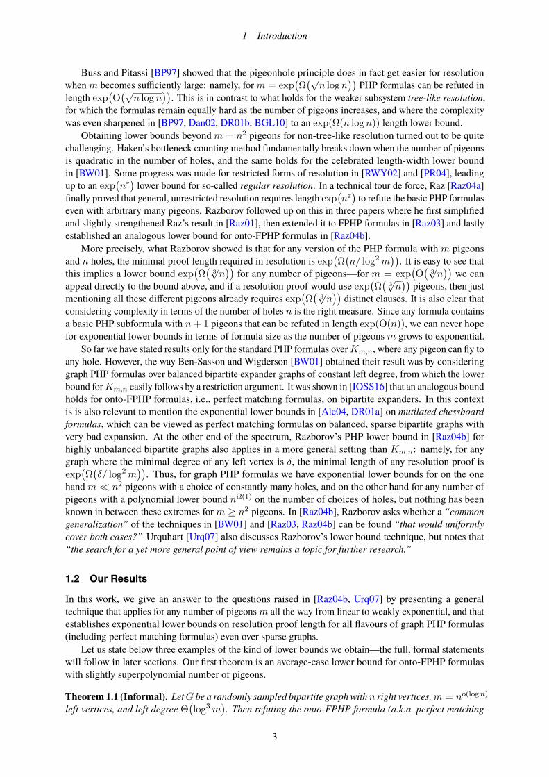
Buss and Pitassi [BP97] showed that the pigeonhole principle does in fact get easier for resolutionwhen m becomes sufficiently large: namely, for m = exp

(Ω(√n log n

))PHP formulas can be refuted in

length exp(O(√n log n

)). This is in contrast to what holds for the weaker subsystem tree-like resolution,

for which the formulas remain equally hard as the number of pigeons increases, and where the complexitywas even sharpened in [BP97, Dan02, DR01b, BGL10] to an exp(Ω(n log n)) length lower bound.

Obtaining lower bounds beyond m = n2 pigeons for non-tree-like resolution turned out to be quitechallenging. Haken’s bottleneck counting method fundamentally breaks down when the number of pigeonsis quadratic in the number of holes, and the same holds for the celebrated length-width lower boundin [BW01]. Some progress was made for restricted forms of resolution in [RWY02] and [PR04], leadingup to an exp

(nε)

lower bound for so-called regular resolution. In a technical tour de force, Raz [Raz04a]finally proved that general, unrestricted resolution requires length exp

(nε)

to refute the basic PHP formulaseven with arbitrary many pigeons. Razborov followed up on this in three papers where he first simplifiedand slightly strengthened Raz’s result in [Raz01], then extended it to FPHP formulas in [Raz03] and lastlyestablished an analogous lower bound for onto-FPHP formulas in [Raz04b].

More precisely, what Razborov showed is that for any version of the PHP formula with m pigeonsand n holes, the minimal proof length required in resolution is exp

(Ω(n/ log2m

)). It is easy to see that

this implies a lower bound exp(Ω(

3√n))

for any number of pigeons—for m = exp(O(

3√n))

we canappeal directly to the bound above, and if a resolution proof would use exp

(Ω(

3√n))

pigeons, then justmentioning all these different pigeons already requires exp

(Ω(

3√n))

distinct clauses. It is also clear thatconsidering complexity in terms of the number of holes n is the right measure. Since any formula containsa basic PHP subformula with n+ 1 pigeons that can be refuted in length exp(O(n)), we can never hopefor exponential lower bounds in terms of formula size as the number of pigeons m grows to exponential.

So far we have stated results only for the standard PHP formulas overKm,n, where any pigeon can fly toany hole. However, the way Ben-Sasson and Wigderson [BW01] obtained their result was by consideringgraph PHP formulas over balanced bipartite expander graphs of constant left degree, from which the lowerbound forKm,n easily follows by a restriction argument. It was shown in [IOSS16] that an analogous boundholds for onto-FPHP formulas, i.e., perfect matching formulas, on bipartite expanders. In this contextis is also relevant to mention the exponential lower bounds in [Ale04, DR01a] on mutilated chessboardformulas, which can be viewed as perfect matching formulas on balanced, sparse bipartite graphs withvery bad expansion. At the other end of the spectrum, Razborov’s PHP lower bound in [Raz04b] forhighly unbalanced bipartite graphs also applies in a more general setting than Km,n: namely, for anygraph where the minimal degree of any left vertex is δ, the minimal length of any resolution proof isexp(Ω(δ/ log2m

)). Thus, for graph PHP formulas we have exponential lower bounds for on the one

hand m n2 pigeons with a choice of constantly many holes, and on the other hand for any number ofpigeons with a polynomial lower bound nΩ(1) on the number of choices of holes, but nothing has beenknown in between these extremes for m ≥ n2 pigeons. In [Raz04b], Razborov asks whether a “commongeneralization” of the techniques in [BW01] and [Raz03, Raz04b] can be found “that would uniformlycover both cases?” Urquhart [Urq07] also discusses Razborov’s lower bound technique, but notes that“the search for a yet more general point of view remains a topic for further research.”

1.2 Our Results

In this work, we give an answer to the questions raised in [Raz04b, Urq07] by presenting a generaltechnique that applies for any number of pigeons m all the way from linear to weakly exponential, and thatestablishes exponential lower bounds on resolution proof length for all flavours of graph PHP formulas(including perfect matching formulas) even over sparse graphs.

Let us state below three examples of the kind of lower bounds we obtain—the full, formal statementswill follow in later sections. Our first theorem is an average-case lower bound for onto-FPHP formulaswith slightly superpolynomial number of pigeons.

Theorem 1.1 (Informal). LetG be a randomly sampled bipartite graph withn right vertices,m = no(logn)

left vertices, and left degree Θ(log3m

). Then refuting the onto-FPHP formula (a.k.a. perfect matching

3


formula) over G in resolution requires length exp(Ω(n1−o(1)

))asymptotically almost surely.

Note that as the number of pigeons grow larger, it is clear that the left degree also has to grow—otherwise we will get a small number of pigeons constrained to fly to a small number of holes by a birthdayparadox argument, yielding a small unsatisfiable subformula that can easily be refuted by brute force.

If the number of pigeons increases further to weakly exponential, then randomly sampled graphs nolonger have good enough expansion for our technique to work, but there are explicit constructions ofunbalanced expanders for which we can still get lower bounds.

Theorem 1.2 (Informal). There are explicitly constructible bipartite graphs G with n right vertices,m = exp

(O(n1/16

))left vertices, and left degree Θ

(log4m

)such that refuting the perfect matching

formula over G requires length exp(Ω(n1/8−ε)) in resolution.

Finally, for functional pigeonhole principle formulas we can also prove an exponential lower bound forconstant left degree even if the number of pigeons is a large polynomial.

Theorem 1.3 (Informal). Let G be a randomly sampled bipartite graph with n right vertices, m = nk

left vertices, and left degree Θ((k/ε)2

). Then refuting the functional pigeonhole principle formula overG

in resolution requires length exp(Ω(n1−ε)) asymptotically almost surely.

1.3 Techniques

At a very high level, what we do in terms of techniques is to revisit the pseudo-width method introducedby Razborov for functional PHP formulas in [Raz03]. We strengthen this method to work in the settingof sparse graphs by combining it with the closure operation on expander graphs in [AR03, ABRW04],which is a way to restore expansion after a small set of (potentially adversarially chosen) vertices havebeen removed. To extend the results further to perfect matching formulas, we apply a “preprocessing step”on the formulas as in [Raz04b]. In what remains of this section, we focus on graph FPHP formulas andgive an informal overview of the lower bound proof in this setting, which already contains most of theinteresting ideas (although the extension to onto-FPHP also raises significant additional challenges).

Let FPHP(G) denote the functional pigeonhole principle formula over the graph G consisting ofclauses (1.1a)–(1.1c). A first, quite naive (and incorrect), description of the proof structure is that westart by defining a pseudo-width measure on clauses C that counts pigeons i that appear in C in manyvariables xij for distinct j. We then show that any short resolution refutation of FPHP(G) can betransformed into a refutation where all clauses have small pseudo-width. By a separate argument, weestablish that any refutation of FPHP(G) requires large pseudo-width. Hence, no short refutations canexist, which is precisely what we were aiming to prove.

To fill in the details (and correct) this argument, let us start by making clear what we mean by pseudo-width. Suppose that the graph G has left degree ∆. In what follows, we identify a mapping of pigeon ito a neighbouring hole j with the partial assignment ρ such that ρ(xi,j) = 1 and ρ(xi,j′) = 0 for allj′ ∈ N(i) \ j. We denote by di(C) the number of mappings of pigeon i that satisfy C. Note that ifC contains at least one negated literal xi,j , then di(C) ≥ ∆ − 1, and otherwise di(C) is the numberof positive literals xi,j for j ∈ N(i). Given a judiciously chosen “filter vector” ~d = (d1, . . . , dm) fordi ≈ ∆ and a “slack” δ ≈ ∆/ logm, we say that pigeon i is heavy in C if di(C) ≥ di−δ and super-heavyif di(C) ≥ di. We define the pseudo-width of a clause C to be be the number of heavy pigeons in C.

With these definitions in hand, we can give a description of the actual proof:

1. Given any resolution refutation π of FPHP(G) in small length L, we argue that all clauses can beclassified as having either low or high pseudo-width, where an important additional guarantee is thatthe high-width clauses not only have many heavy pigeons but actually many super-heavy pigeons.

2. We replace all clauses C with many super-heavy pigeons with “fake axioms” C ′ ⊆ C obtainedby throwing away literals from C until we have nothing left but a medium number of super-heavypigeons. By construction, the set A of such fake axioms is of size |A| ≤ L, and after making thereplacement we have a resolution refutation π′ of FPHP(G) ∪ A in low pseudo-width.

4

1 Introduction

3. However, sinceA is not too large, we are able to show that any resolution refutation ofFPHP(G)∪Amust still require large pseudo-width. Hence, L cannot be small, and the lower bound follows.

Part 1 is similar to [Raz03], but with a slight twist. We show that if the length of π is L < 2w0 andif we choose δ ≤ ε∆ log n/ logm, then there exists a vector ~d = (d1, . . . , dm) such that for all clausesin π either the number of super-heavy pigeons is at least w0 or else the number of heavy pigeons isat most O

(w0 · nε

). The proof of this is by sampling the coordinates di independently from a suitable

probability distribution and then applying a union bound argument. Once this has been established, part 2follows easily: we just replace all clauses with at least w0 super-heavy pigeons by (stronger) fake axioms.Including all fake axioms A yields a refutation π′ of FPHP(G) ∪ A (since we can add a weakeningrule deriving C from C ′ ⊆ C to resolution without loss of generality) and clearly all clauses in π′ havepseudo-width O

(w0 · nε

).

Part 3 is where most of the hard work is. Suppose that G is an excellent expander graph, so thatall left vertex sets U ′ of size

∣∣U ′∣∣ ≤ r have at least (1− ε log n/logm)∆|U ′| unique neighbours on theright-hand side. We show that under the assumptions above, refuting FPHP(G)∪A requires pseudo-widthΩ(r · log n/logm

). Tuning the parameters appropriately, this yields a contradiction with part 2.

Before outlining how the proof of part 3 goes, we remark that the requirements we place on theexpansion of G are quite severe. Clearly, any left vertex set U can have at most ∆|U ′| neighbours in total,and we are asking for all except a vanishingly small fraction of these neighbours to be unique. This iswhy we can etablish Theorem 1.1 but not Theorem 1.2 for randomly sampled graphs. We see no reasonto believe that the latter theorem would not hold also for random graphs, but the expansion propertiesrequired for our proof are so stringent that they are not satisfied in this parameter regime. This seemsto be a fundamental shortcoming of our technique, and it appears that new ideas would be required tocircumvent this problem.

In order to argue that refuting FPHP(G) ∪ A in resolution requires large pseudo-width, we wantto estimate how much progress the resolution derivation has made up to the point when it derives someclause C. Following Razborov’s lead, we measure this by looking at what fraction of partial matchingsof all the heavy pigeons in C do not satisfy C (meaning, intuitively, that the derivation has managed torule out this part of the search space). It is immediate by inspection that all pigeons mentioned in the realaxiom clauses (1.1a)–(1.1c) are heavy, and any matching of such pigeons satisfies the clauses. Thus, theoriginal axioms in FPHP(G) do not rule out any matchings. Also, it is easy to show that fake axioms ruleout only an exponentially small fraction of matchings, since they contain many super-heavy pigeons andit is hard to match all of these pigeons without satisfying the clause. However, the contradictory emptyclause⊥ rules out 100% of partial matchings, since it contains no heavy pigeons to match in the first place.

What we would like to prove now is that for any derivation in small pseudo-width it holds that thederived clause cannot rule out any matching other than those already eliminated by the clauses used toderive it. This means that the fake axioms together need to rule out all partial matchings, but since everyfake axiom contributes only an exponentially small fraction they are too few to achieve this. Hence, it isnot possible to derive contradiction in small pseudo-width, which completes part 3 of our proof outline.

There is one problem, however: the last claim above is not true, and so what is outlined above is onlya fake proof. While we have to defer the discussion of what the full proof actually looks like in detail, weconclude this section by attempting to hint at a couple of technical issues and how to resolve them.

Firstly, it does not hold that a derived clause C eliminates only those matchings that are also forbiddenby one of the predecessor clauses used to derive C. The issue is that a pigeon i that is heavy in bothpredecessors might cease to be heavy in C—for instance, if C was derived by a resolution step over avariable xi,j . If this is so, then we would need to show that any matching of the heavy pigeons in C canbe extended to match also pigeon i to any of its neighbouring holes without satisfying both predecessorclauses. But this will not be true, because a non-heavy pigeon can still have some variable xi,j occurringin both predecessors. The solution to this, introduced in [Raz03], is to do a “lossy counting” of matchingsby associating each partial matching with a linear subspace of some suitable vector space, and then toconsider the span of all matchings ruled out by C. When we accumulate a “large enough” number ofmatchings for a pigeon i, then the whole subspace associated to i is spanned and we can stop counting.

5


But this leads to a second problem: when studying matchings of the heavy pigeons in C we mightalready have assigned pigeons i′1, . . . , i′w that occupy holes where pigeon i might want to fly. For standardPHP formulas over complete bipartite graphs this is not a problem, since at least n − w holes are stillavailable and this number is “large enough” in the sense described above. But for a sparse graph it willtypically be the case that w ∆, and so it might well be the case that pigeons i′1, . . . , i′w are alreadyoccupying all the ∆ holes available for pigeon i according to G. Although it is perhaps hard to see fromour (admittedly somewhat informal) discussion, this turns out to be a very serious problem, and indeed itis one of the main technical challenges we need to overcome.

To address this problem we consider not only the heavy pigeons inC, but also any other pigeons inG thatrisk becoming far too constrained when the heavy pigeons ofC are matched. Inspired by [AR03, ABRW04],we define the closure to be a superset S of the heavy pigeons such that when S and the neighbouring holesof S are removed it holds that the residual graph is still guaranteed to be a good expander. Provided that Gis an excellent expander to begin with, and that the number of heavy pigeons in C is not too large, it canthen be shown that an analogue of the original argument outlined above goes through.

1.4 Outline of This Paper

We review the necessary preliminaries in Section 2 and introduce two crucial technical tools in Section 3.The lower bounds for weak graph FPHP formulas are then presented in Section 4, after which the perfectmatching lower bounds follow in Section 5. We conclude with a discussion of questions for future researchin Section 6.

2 Preliminaries

We denote natural logarithms (base e) by ln, and base 2 logarithms by log. For positive integers n ∈ N+

we write [n] = 1, . . . , n.A literal over a Boolean variable x is either the variable x itself (a positive literal) or its negation x (a

negative literal). A clause C = `1 ∨ · · · ∨ `w is a disjunction of literals. We write ⊥ to denote the emptyclause without any literals. A CNF formula F = C1 ∧ · · · ∧ Cm is a conjunction of clauses. We think ofclauses and CNF formulas as sets: order is irrelevant and there are no repetitions. We let Vars(F ) denotethe set of variables of F .

A resolution refutation π of an unsatisfiable CNF formulaF , or resolution proof for (the unsatisfiabilityof) F , is an ordered sequence of clauses π = (D1, . . . , DL) such that DL = ⊥ and for each i ∈ [L] eitherDi is a clause in F (an axiom) or there exist j < i and k < i such that Di is derived from Dj and Dk bythe resolution rule

B ∨ x C ∨ xB ∨ C . (2.1)

We refer to B ∨ C as the resolvent of B ∨ x and C ∨ x over x, and to x as the resolved variable. Fortechnical reasons it is sometimes convenient to also allow clauses to be derived by the weakening rule

CD

[C ⊆ D] (2.2)

(and for two clauses C ⊆ D we will sometimes refer to C as a strengthening of D).The length L(π) of a refutation π = (D1, . . . , DL) isL. The length of refutingF is minπ:F `⊥L(π),

where the minimum is taken over all resolution refutations π of F . It is easy to show that removing theweakening rule (2.2) does not increase the refutation length.

A partial assignment or a restriction on a formula F is a partial function ρ : Vars(F )→ 0, 1. Theclause C restricted by ρ, denoted Cρ, is the trivial 1-clause if any of the literals in C is satisfied by ρand otherwise it is C with all falsified literals removed. We extend this definition to CNF formulas in theobvious way by taking unions. For a variable x ∈ Vars(F ) we write ρ(x) = ∗ if x /∈ dom(ρ), i.e., if ρdoes not assign a value to x.

6

2 Preliminaries

We write G = (V,E) to denote a graph with vertices V and edges E, where G is always undirectedand without loops or multiple edges. Moreover, for bipartite graphs we write G = (U

.∪ V,E), where

edges in E have one endpoint in the left vertex set U and the other in the right vertex set V . A partialmatching ϕ in G is a subset of edges that are vertex-disjoint. Let V (ϕ) = v | ∃e ∈ ϕ : v ∈ e be thevertices of ϕ and for v ∈ V (ϕ) denote by ϕv the unique vertex u such that u, v ∈ ϕ. A vertex v iscovered by ϕ if v ∈ V (ϕ). If ϕ is a partial matching in a bipartite graph G = (U

.∪ V,E), we identify it

with a partial mapping of U to V . When referring to the pigeonhole formula, this mapping will also beidentified with an assignment ρϕ to the variables defined by

ρϕ(xi,j) =

∗ if i /∈ dom(ϕ),0 if i ∈ dom(ϕ) and ϕ(i) 6= j,1 if i ∈ dom(ϕ) and ϕ(i) = j.

(2.3)

Given a vertex v ∈ V(G), we write NG(v) to denote the set of neighbours of v in the graph G and∆G(v) = |NG(v)| to denote the degree of v. We extend this notion to sets and denote by NG(S) =v | ∃ (u, v) ∈ E for u ∈ S the neighbourhood of a set of vertices S ⊆ V . The boundary, or uniqueneighbourhood, ∂G(S) = v ∈ V \S : |NG(v)∩S| = 1 of a set of vertices S ⊆ V contains all verticesin V \S that have a single neighbour in S. If the graph is bipartite, there is of course no need to subtract Sfrom the neighbour set. We will sometimes drop the subscript G when the graph is clear from context.For a set U ⊆ V we denote by G \ U the subgraph of G induced by the vertex set V \ U .

A graph G = (V,E) is an (r,∆, c)-expander if all vertives v ∈ V have degree at most ∆ and for allsets S ⊆ V , |S| ≤ r, it holds that |N(S) \ S| ≥ c · |S|. Similarly, G = (V,E) is an (r,∆, c)-boundaryexpander if all vertices v ∈ V have degree at most ∆ and for all sets S ⊆ V , |S| ≤ r, it holds that|∂(S)| ≥ c · |S|. For bipartite graphs, the degree and expansion requirements only apply to the left vertexset: G = (U

.∪ V,E) is an (r,∆, c)-bipartite expander if all vertices u ∈ U have degree at most ∆ and

for all sets S ⊆ U , |S| ≤ r, it holds that |N(S)| ≥ c · |S|, and an (r,∆, c)-bipartite boundary expanderif for all sets S ⊆ U , |S| ≤ r, it holds that |∂(S)| ≥ c · |S|. For bipartite graphs we will only ever beinterested in bipartite notions of expansions, and so which kind of expansion is meant will always be clearfrom context. A simple but useful observation is that

|N(S) \ S| ≤ |∂(S)|+ ∆|S| − |∂(S)|2

=∆|S|+ |∂(S)|

2, (2.4)

since all non-unique neighbours in N(S) \ S have at least two incident edges. This implies that if a graphG is an (r,∆, (1− ξ)∆)-expander then it is also an (r,∆, (1− 2ξ)∆)-boundary expander.

We often denote random variables in boldface and write X ∼ D to denote that X is sampled from thedistribution D. We will use the following standard forms of the multiplicative Chernoff bounds: if S is asum of independent 0-1 random variables (not necessarily equidistributed) with expectation µ = E[S], thenfor δ ≥ 0 we have that Pr

[µ− S ≥ δ

]≤ exp

(− δ2

2µ

)and Pr

[S − µ ≥ δ

]≤ exp

(− δ2

2µ+δ

). Combining

these two inequalities yields the following statement.

Theorem 2.1. Let S be the sum of independent 0-1 random variables (not necessarily equidistributed)with expectation µ = E[S]. Then for δ ≥ 0 it holds that

Pr[|S − µ| ≥ δ

]≤ 2 exp

(− δ2

2µ+ δ

).

For n,m,∆ ∈ N, we denote by G(m,n,∆) the distribution over bipartite graphs with disjoint vertexsets U = u1, . . . , um and V = v1, . . . , vn where the neighbourhood of a vertex u ∈ U is chosenby sampling a subset of size ∆ uniformly at random from V . A property is said to hold asymptoticallyalmost surely on G(f(n), n,∆) if it holds with probability that approaches 1 as n approaches infinity.

For the right parameters, a randomly sampled graph G ∼ G(m,n,∆) is asymptotically almost surelya good boundary expander as stated next.

7


Lemma 2.2. Let m,n and ∆ be large enough integers such that m > n ≥ ∆. Let ξ, χ ∈ R+ be suchthat ξ < 1/2, ξ lnχ ≥ 2 and ξ∆ lnχ ≥ 4 lnm. Then for r = n/(∆ · χ) and c = (1 − 2ξ)∆ itholds asymptotically almost surely for a randomly sampled graphG ∼ G(m,n,∆) thatG is an (r,∆, c)-boundary expander.

Proof. Let G = (U.∪ V,E). We first estimate the probability that a set S ⊆ U of size at most r violates

the boundary expansion. For brevity, let us write s = |S| and c′ = (1 − ξ)∆. In view of (2.4), theprobability that S violates the boundary expansion can be bounded by

Pr[|∂(S)| < cs

]≤ Pr

[|N(S)| < ∆s+ cs

2

](2.5a)

= Pr[|N(S)| < c′s

](2.5b)

≤(n

c′s

)·

((c′s∆

)(n∆

) )s (2.5c)

≤(n

c′s

)·(c′s

n

)∆s

(2.5d)

≤

[( enc′s

)c′·(c′s

n

)∆]s

(2.5e)

=

[e(1−ξ)∆ ·

( nc′s

)−ξ∆]s(2.5f)

≤ exp(

∆s(

1− ξ ln( nc′s

)))(2.5g)

≤ exp

(∆s

(1− ξ ln

(χ

1− ξ

)))(2.5h)

≤ exp (∆s(1− ξ lnχ)) (2.5i)≤ exp (−(∆sξ lnχ)/2) , (2.5j)

where (2.5h) holds since s ≤ r ≤ n/(∆χ) and (2.5j) holds since ξ lnχ ≥ 2. Hence, the probability thatG is not a boundary expander can be bounded by

Pr[G is not an expander

]≤∑s∈[r]

(m

s

)exp(−(∆sξ lnχ)/2)

≤∑s∈[r]

exp(−s((ξ∆ lnχ)/2− lnm)) (2.6)

≤∑s∈[r]

exp(−s lnm) ≤ 1

m− 1,

where the second-to-last inequality holds since ξ∆ lnχ ≥ 4 lnm.

We will also need to consider some parameter settings where randomly sampled graphs do not havestrong enough expansion for our purposes, but where we can resort to explicit constructions as follows.

Theorem 2.3 ([GUV09]). For all positive integers m, r ≤ m, all ξ > 0, and all constant ν > 0,there is an explicit (r,∆, (1 − ξ)∆)-expander G = (U

.∪ V,E), with |U | = m, |V | = n, ∆ =

O(((logm)(log r)/ξ)1+1/ν

)and n ≤ ∆2 · r1+ν .

Corollary 2.4. Let κ, ε, ν be positive constants, κ < 18 , and let n be a large enough integer. Then there

is an explicit graphG = (U.∪V,E), with |U | = m = 2Ω(nκ) and |V | ≤ n, that is an (n

11+ν− 4κν ,∆, (1−

2ξ)∆)-boundary expander for ξ = ε lognlogm and ∆ = O(log2(1+1/ν)m).

8

3 Two Key Technical Tools

Proof. Let G be the expander from Theorem 2.3 for the parameters m = 2ε′nκ , r = n

11+ν− 4κν , and

ξ = ε lognlogm , where ε′ is chosen to be a small enough constant so that ∆2 · r1+ν ≤ n. Such a graph G is an

(r,∆, (1− ξ)∆)-expander for ∆ as in the Corollary. By (2.4) it follows that an (r,∆, c)-expander is an(r,∆, 2c−∆)-boundary expander, and hence G is an

(r,∆, (1− 2ξ)∆

)-boundary expander. Note that

Theorem 2.3 guarantees that the right side of G has size at most ∆2 · r1+ν ≤ n.


In this section we review two crucial technical ingredients in the resolution lower bound proofs.

3.1 Pigeon Filtering

The following lemma is a generalization of [Raz03, Lemma 6]. The difference is that we have an additionalparameter α (which is implicitly fixed to α = 2 in [Raz03]) that allows us to get a better upper bound onthe numbers ri. This turns out to be crucial for us—we discuss this in more detail in Section 4.

Lemma 3.1 (Filter lemma). Let m,L ∈ N+ and suppose that w0, α ∈ [m] are such that w0 > lnL andw0 ≥ α2 ≥ 4. Further, let ~r(1), . . . , ~r(L) be integer vectors, each of the form ~r(`) = (r1(`), . . . , rm(`)).Then there exists a vector ~r = (r1, . . . , rm) of positive integers ri ≤

⌊ logmlogα

⌋− 1 such that for all ` ∈ [L]

at least one of the following holds:1.∣∣i ∈ [m] : ri(`) ≤ ri

∣∣ ≥ w0 ,

2.∣∣i ∈ [m] : ri(`) ≤ ri + 1

∣∣ ≤ O(α · w0) .

Proof. We first define a weight function W (~r) for vectors ~r = (r1, . . . , rm) as

W (~r) =∑i∈[m]

α−ri . (3.1)

In order to establish the lemma, it is sufficient to show that there exist constants γ and γ′ and a vectorr = (r1, . . . , rm) such that for all ` ∈ [L] the implications

W (~r(`)) ≥ γ′w0

α⇒ |i ∈ [m] | ri ≥ ri(`)| ≥ w0 , (3.2a)

W (~r(`)) ≤ γ′w0

α⇒ |i ∈ [m] | ri ≥ ri(`)− 1| ≤ γαw0 (3.2b)

hold. Let t =⌊ logm

logα

⌋− 1 and let µ be a probability distribution on [t] given by Pr[rrr = i] = β · α−i for

all i ∈ [t], where β = α−11−α−t . Note that

β∑i∈[t]

α−i =α− 1

1− α−t

(1− α−t

α− 1

)= 1 (3.3)

and thus µ is a valid distribution. Let us write~r~r~r = (r1r1r1, . . . , rmrmrm) to denote a random vector with coordinatessampled independently according to µ. We claim that for every ` ∈ [L] the implications (3.2a) and (3.2b)are true asymptotically almost surely. Let us proceed to verify this.

1. Suppose that W (~r(`)) ≥ γ′w0

α . We wish to show that |i ∈ [m] : ri ≥ ri(`)| ≥ w0. Observe thatcoordinates larger than t contribute only∑

ri(`)>t

α−ri(`) ≤ m · α−t−1 < α (3.4)

9


to W (~r(`)), and hence the weight function truncated at t is∑ri(`)≤t

α−ri(`) ≥ γ′w0

α− α ≥ (γ′ − 1)

w0

α, (3.5)

since w0 ≥ α2. Note that for every coordinate i with ri(`) ≤ t we have that Pr[ririri ≥ ri(`)] ≥β · α−ri(`). Consider the random set P~r~r~r(`) = i ∈ [m] | ri(`) ≤ t and ririri ≥ ri(`). We can appealto (3.5) to derive that

E[|P~r~r~r(`)|

]=∑ri(`)≤t

Pr[ririri ≥ ri(`)] ≥∑ri(`)≤t

βα−ri(`) ≥ β(γ′ − 1)w0

α≥ γ′ − 1

2w0 (3.6)

is a lower bound on the expected size of P~r~r~r(`). As the events ririri ≥ ri(`) are independent, by themultiplicative Chernoff bound we get that

Pr[|P~r~r~r(`)| < w0

]≤ Pr

[|P~r~r~r(`)| − E

[|P~r~r~r(`)|

]≤ w0 − E

[|P~r~r~r(`)|

]](3.7a)

= Pr[E[|P~r~r~r(`)|

]− |P~r~r~r(`)| ≥ E

[|P~r~r~r(`)|

]− w0

](3.7b)

≤ exp(−(E[|P~r~r~r(`)|

]− w0

)22 E[|P~r~r~r(`)|

] )(3.7c)

= exp

(−

E[|P~r~r~r(`)|

]2 − 2 E[|P~r~r~r(`)|

]w0 + w2

0

2 E[|P~r~r~r(`)|

] )(3.7d)

≤ exp

(−

E[|P~r~r~r(`)|

]− 2w0

2

)(3.7e)

≤ exp

(−(γ′ − 5)

4w0

)(3.7f)

≤ exp(−2w0) (3.7g)≤ L−2 , (3.7h)

where the second to last inequality holds for γ′ ≥ 13.

2. Suppose that W (~r(`)) ≤ γ′w0

α . Now we need to show that |i ∈ [m] : ri ≥ ri(`) − 1| ≤ γαw0

holds asymptotically almost surely. Note that

Pr[ririri ≥ ri(`)− 1] = βt∑

j=ri(`)−1

α−j (3.8a)

=α− 1

1− α−t

(α−ri(`)+2 − α−t

α− 1

)(3.8b)

=α−ri(`)+2 − α−t

1− α−t(3.8c)

=αt−ri(`)+2 − 1

αt − 1(3.8d)

≤ αt−ri(`)+2

αt/2= 2α2−ri(`) . (3.8e)

Similar to the previous case, let Q~r~r~r(`) = i ∈ [m] | ririri ≥ ri(`) − 1. We can upper-bound theexpected cardinality of Q~r~r~r(`) by

E[|Q~r~r~r(`)|

]=∑i∈[m]

Pr[ririri ≥ ri(`)− 1] ≤ 2α2W (~r(`)) ≤ 2γ′αw0 . (3.9)

10


Again, we apply the Chernoff bound in Theorem 2.1 and conclude that

Pr[|Q~r~r~r(`)| ≥ γαw0

]≤ Pr

[|Q~r~r~r(`)| − E

[|Q~r~r~r(`)|

]≥ γαw0 − 2γ′αw0

]≤ exp

(− (γ − 2γ′)2(αw0)2

4γ′αw0 + (γ − 2γ′)αw0

)(3.10)

≤ exp(−αw0)

≤ L−2

where the second to last inequality holds for γ sufficiently larger than γ′, say γ ≥ 5γ′.

A union bound argument over all vectors in ~r(`) : ` ∈ [L] for both cases shows that for γ′ ≥ 13 andγ ≥ 5γ′ there exists a choice of ~r = (r1, . . . , rm) such that both implications (3.2a) and (3.2b) hold.

3.2 Graph Closure

A key concept in our work will be that of a closure of a vertex set, which seems to have originatedin [AR03, ABRW04]. Intuitively, for an expander graph G, the closure of T ⊆ V (G) is a suitably smallset S that contains T such that G \ S is an expander. In order to have a definition that makes sense forboth expanders and bipartite expanders, we define Vexp(G) to be the set of vertices of G that expand, thatis, if G = (V,E) is an expander then Vexp(G) = V , and if G = (U

.∪ V,E) is a bipartite expander then

Vexp(G) = U .

Definition 3.2 (Closure). For an expander graph G and vertex sets S ⊆ Vexp(G) and U ⊆ V (G), we saythat the set S is (U, r, ν)-contained if |S| ≤ r and

∣∣∂(S) \ U∣∣ < ν · |S|.

For any expander graph G and any set T ⊆ Vexp(G) of size |T | ≤ r, we will let closurer,ν(T )denote an arbitrary but fixed maximal set such that T ⊆ closurer,ν(T ) ⊆ Vexp(G) and closurer,ν(T ) is(N(T ), r, ν)-contained.

Note that the closure of any set T of size |T | ≤ r as defined above does indeed exist, since T itself is(N(T ), r, ν)-contained.

Lemma 3.3. Suppose that G is an (r,∆, c)-boundary expander and that T ⊆ Vexp(G) has size |T | ≤k ≤ r. Then |closurer,ν(T )| < k∆

c−ν .

Proof. By definition we have that∣∣∂(closurer,ν(T )) \N(T )

∣∣ < ν · |closurer,ν(T )|. Furthermore, since|closurer,ν(T )| ≤ r by definition, we can use the expansion property of the graph to derive the inequality∣∣∂(closurer,ν(T )) \N(T )

∣∣ ≥ |∂(closurer,ν(T ))| − |N(T )| ≥ c · |closurer,ν(T )| − k∆. Note that we alsouse the fact that the neighbourhood of T is of size at most k∆. The conclusion follows by combining bothstatements.

Suppose G is an excellent boundary expander and that T ⊆ Vexp(G) is not too large. Then Lemma 3.3shows that the closure of T is not much larger. And if the closure is not too large, then after removingthe closure and its neighbourhood from the graph we are still left with a decent expander, a fact whichwill play a key role in the technical arguments in later sections. The following lemma makes this intuitionprecise.

Lemma 3.4. For G an (r,∆, c)-boundary expander, let T ⊆ Vexp(G) be such that |T | ≤ r and|closurer,ν(T )| ≤ r/2, letG′ = G\

(closurer,ν(T )∪N(closurer,ν(T ))

)andVexp(G′) = Vexp(G)∩V (G′).

Then any set S ⊆ Vexp(G′) of size |S| ≤ r/2 satisfies |∂G′(S)| ≥ ν|S|.

Proof. Suppose the set S ⊆ Vexp(G′) is of size |S| ≤ r/2 and does not satisfy |∂G′(S)| ≥ ν|S|. Sinceclosurer,ν(T ) is also of size at most r/2, we have that the set (closurer,ν(T )∪S) is (N(T ), r, ν)-containedin the graph G. But this contradicts the maximality of closurer,ν(T ).

11


4 Lower Bounds for Weak Graph FPHP Formulas

We now proceed to establish lower bounds on the length of resolution refutations of functional pigeonholeprinciple formulas defined over bipartite graphs. We write G = (VP

.∪ VH , E) to denote the graph over

which the formulas are defined andM to denote the set of partial matchings on G (also viewed as partialmappings of VP to VH ). Let us start by making more precise some of the technical notions discussed inthe introduction (which were originally defined in [Raz01]).

For a clause C and a pigeon i we denote the set of holes j with the property that C is satisfied if i ismatched to j by

NC(i) = j ∈ VH | e = i, j ∈ E and ρe(C) = 1 (4.1)

and we define the ith pigeon degree ∆C(i) of C as

∆C(i) = |NC(i)| . (4.2)

We think of a pigeon i with large ∆C(i) as a pigeon on which the derivation has not made any significantprogress up to the point of deriving C, since the clause rules out very few holes. The pigeons with highenough pigeon degree in a clause are the heavy pigeons of the clause as defined next.

Definition 4.1 (Pigeon weight, pseudo-width and(w0, ~d

)-axioms). Let C be a clause and let ~d =

(d1, . . . , dm) and ~δ = (δ1, . . . , δm) be two vectors of positive integers such that ~d is elementwise greaterthan ~δ. We say that pigeon i is ~d-super-heavy for C if ∆C(i) ≥ di and that pigeon i is (~d, ~δ)-heavy for Cif ∆C(i) ≥ di − δi. When ~d and ~δ are understood from context, which is most often the case, we omit theparameters and just refer to super-heavy and heavy pigeons. Pigeons that are not heavy are referred to aslight pigeons. The set of pigeons that are super-heavy for C is denoted by

P~d(C) = i ∈ [m] | ∆C(i) ≥ di

and the set of pigeons that are heavy for C is denoted by

P~d,~δ(C) = i ∈ [m] | ∆C(i) ≥ di − δi .

The pseudo-width ofC is the number of heavy pigeons inC and the pseudo-width of a resolution refutationπ, denoted by w~d,~δ(π), is maxC∈π w~d,~δ(C). Finally, we will refer to clauses C with precisely w0 super-heavy pigeons, i.e., such that |P~d(C)| = w0, as

(w0, ~d

)-axioms.

Note that according to Definition 4.1 super-heavy pigeons are also heavy. Making the connection backto our informal discussion in the introduction, the “fake axioms” mentioned there are nothing other than(w0, ~d

)-axioms.

Now that we have all the notions needed, let us give a detailed proof outline. Given a short resolutionrefutation π of the formula FPHP(G), we use the Filter lemma (Lemma 3.1) to get a filter vector~d = (d1, . . . , dm) such that each clause either has many super-heavy pigeons or there are not too manyheavy pigeons (for an appropriately chosen vector ~δ). Clearly, clauses that fall into the second case of thefilter lemma have bounded pseudo-width. On the other hand, clauses in the first case may have very largepseudo-width. In order to obtain a proof of low pseudo-width, these clauses are strengthened to

(w0, ~d

)-

axioms and added to a special setA. This then gives a refutation π′ that refutes the formula FPHP(G)∪Ain bounded pseudo-width. The following lemma summarizes the upper bound on pseudo-width that weobtain.

Lemma 4.2. Let G = (VP.∪ VH , E) be a bipartite graph with |VP | = m and |VH | = n; let π be a

resolution refutation of FPHP(G); let w0, α ∈ [m] be such that w0 > logL(π) and w0 ≥ α2 ≥ 4, andlet ~δ = (δ1, . . . , δm) be defined by δi = ∆G(i) logα

logm . Then there exists an integer vector ~d = (d1, . . . , dm),with δi < di ≤ ∆G(i) for all i ∈ VP , a set of

(w0, ~d

)-axioms A with |A| ≤ L(π), and a resolution

refutation π′ of FPHP(G) ∪ A such that w~d,~δ(π′) = O(α · w0).

12


As mentioned above, this upper bound is a straightforward application of Lemma 3.1. We deferthe formal proof to Section 4.2. What we will need from Lemma 4.2 is that a resolution refutation ofFPHP(G) in length less than 2w0 can be transformed into a refutation of FPHP(G)∪A in pseudo-widthat most O(α · w0).

The second step in the proof is to show that any resolution refutation π of FPHP(G) ∪ A requireslarge pseudo-width. The high-level idea is to define a progress measure on clauses C ∈ π by countingthe number of matchings on P~d,~δ(C) that do not satisfy C. We then show that in order to increase thisprogress measure we need large pseudo-width. The following lemma states the pseudo-width lower bound.

Lemma 4.3. Let ξ ≤ 1/4 and m,n, r,∆ ∈ N; let G = (VP.∪ VH , E) with |VP | = m and |VH | = n

be an (r,∆, (1 − 2ξ)∆)-boundary expander, and let ~δ = (δ1, . . . , δm) be defined by δi = 4∆G(i)ξ.Suppose that ~d = (d1, . . . , dm) is an integer vector such that δi < di ≤ ∆G(i) for all i ∈ VP . Let w0 bean arbitrary parameter and A be an arbitrary set of

(w0, ~d

)-axioms with |A| ≤ (1 + ξ)w0 . Then every

resolution refutation π of FPHP(G) ∪ A must satisfy w~d,~δ(π) ≥ rξ/4.

In one sentence, the lemma states that if the set of “fake axioms” A is not too large, then resolutionrequires large pseudo-width to refute FPHP(G) ∪ A. Note that this lemma holds for any filter vector andnot just for the one obtained from Lemma 4.2.

In order to prove Lemma 4.3, we wish to define a progress measure on clauses that indicates howclose the derivation is to refuting the formula (i.e., it should be small for axiom clauses but large forcontradiction). A first attempt would be to define the progress of a clause C as the number of ruled-outmatchings (i.e., matchings that do not satisfy C) on the pigeons mentioned by C. This definition does notquite work, but we can refine it by counting matchings less carefully. Namely, if for a pigeon i there aremore than ∆G(i)− di + δi/4 holes to which it can be mapped without satisfying C, then we think of Cas ruling out all holes for this pigeon. Since the pigeon degree of a light pigeon i is at most di − δi, such apigeon will certainly have at least ∆G(i)− di + δi ≥ ∆G(i)− di + δi/4 holes to which it can be mapped,and the “lossy counting” will ensure that all holes are considered as ruled out.

We realize this “lossy counting” through a linear space Λ, in which each partial matching ϕ isassociated with a subspace λ(ϕ). Roughly speaking, the progress λ(C) of a clause C is then defined to bethe span of all partial matchings that are ruled out by C. We design the association between matchings andsubspaces so that the contradictory empty clause ⊥ has λ(⊥) = Λ but so that the span of all the axiomsspan(λ(A) | A ∈ FPHP(G) ∪ A) is a proper subspace of Λ. This implies that in a refutation π ofFPHP(G) ∪ A there must exist a resolution step deriving a clause C from clauses C0 and C1 such thatthe linear space of the resolvent λ(C) is not contained in span(λ(C0), λ(C1)). But the main technicallemma of this section (Lemma 4.10) says that for any derivation in low pseudo-width the linear space ofthe resolvent is contained in the span of the linear spaces of the clauses being resolved. Hence, in orderfor π to be a refutation it must contain a clause with large pseudo-width, and this establishes Lemma 4.3.

So far our argument follows that of Razborov very closely, but it turns out we cannot realize this proofidea if we only keep track of heavy and light pigeons. Let us attempt a proof of the claim in Lemma 4.10that low-width resolution steps cannot increase the span to illustrate what the problem is. The interestingcase is when there is a pigeon i that is heavy for C0 or C1 but not for their resolvent C. Then, followingRazborov, for any matching ϕ on the heavy pigeons of C that fails to satisfy C, we need to be able toextend ϕ in at least ∆G(i)− di + δi/4 different ways to a matching including also pigeon i that falsifieseither C0 or C1. If this can be done, then we think of C0 and C1 as together ruling out (essentially) allholes for i, and the linear space associated with C will be contained in the span of the spaces for C0 andC1. The problem, though, is that ϕ may send all heavy pigeons to the neighbourhood of pigeon i. In thisscenario, there might be very few holes, or even no holes, to which i can be mapped when extending ϕ,and even our lossy counting will not be able to pick up enough holes for the argument to go through.We resolve this problem by not only considering the heavy pigeons but a larger set of relevant pigeonsincluding all pigeons i′ that can become overly constrained when some matching on the heavy pigeonsshrinks the neighbourhood of i′ too much. Formally, the closure of the set of heavy pigeons, as defined inDefinition 3.2, is the notion that we need.

13


4.1 Formal Statements of Graph FPHP Formula Lower Bounds

Deferring the proofs of all technical lemmas for now, let us state our lower bounds for graph FPHP formulasand see how they follow from Lemmas 4.2 and 4.3 above.

Theorem 4.4. Letm = |U | and n = |V | and suppose thatG = (U.∪V,E) is an

(r,∆,

(1− logα

2 logm

)∆)-

boundary expander for α ∈ [m] such that 8 ≤ α3

logα = o(

rlogm

). Then resolution requires length

exp(

Ω(r log2 αα log2m

))to refute FPHP(G).

As promised in Section 3, let us briefly discuss the parameter α. Note that, on the one hand, the largerα is, the more relaxed we can be with respect to the expansion requirements, and hence the set of formulasto which the lower bound applies becomes larger. On the other hand, the strength of the lower bounddeteriorates quickly with α. Hence, we need to choose α carefully to find a good trade-off between thesetwo concerns.

Proof of Theorem 4.4. Let ξ = logα4 logm and let w0 = ε0rξ

α for some small enough ε0 > 0. We note that thechoice of parameters and the condition on α ensure that 4 ≤ α2 ≤ w0. Furthermore, in terms of ξ, thegraph G is an (r,∆, (1− 2ξ)∆)-boundary expander.

We proceed by contradiction. Suppose π is a resolution refutation with L(π) < 2ε′w0ξ for a small

enough constant ε′ > 0. Applying Lemma 4.2 we get a set of(w0, ~d

)-axioms A with |A| ≤ L(π) and a

resolution refutation π′ of FPHP(G)∪A such that w~d,~δ(π′) ≤ Kαw0 for some large enough constant K.

Note that |A| ≤ L(π) < 2ε′w0ξ ≤ (1 + ξ)w0 for ε′ < 1/2. Applying Lemma 4.3 to π′ yields a

pseudo-width lower bound of rξ/4. We conclude that

rξ/4 ≤ w~d,~δ(π′) ≤ Kαw0 = ε0Krξ . (4.3)

Choosing ε0 <1

4K yields a contradiction.

The following corollary summarizes our claims for random graphs.

Corollary 4.5. Let m and n be positive integers and let ∆ : N+ → N+ and ε : N+ → [0, 1] be any

monotone functions of n such that n < m ≤ n(ε/16)2 logn and n ≥ ∆ ≥(

16 logmε logn

)2. Then asymptotically

almost surely resolution requires length exp(Ω(n1−ε)) to refute FPHP(G) for G ∼ G

(m,n,∆

).

Proof. For simplicity, let us assume that n(ε/16)2 logn and((16 logm)/(ε log n)

)2 are integers. Observethat if G ∼ G (m,n,∆) for ∆ >

((16 logm)/(ε log n)

)2, then we can sample a random subgraph G′ ∼G(m,n, ((16 logm)/(ε log n))2

)by choosing a random subset of appropriate size of each neighbourhood

of a left vertex (and applying a restriction zeroing out the other edges). Hence, we can restrict ourattention to the case where ∆ =

((16 logm)/(ε log n)

)2. Also, it is sufficient to prove the claim form = n(ε/16)2 logn, since choosing m smaller can only make the formula less constrained and hence makesthe lower bound easier to obtain.

We want to apply Lemma 2.2 for χ = α = nε/4 and ξ = logα4 logm . In order to do so, we need to verify

the inequalities

ξ < 1/2 , (4.4a)ξ lnχ ≥ 2 , (4.4b)

ξ∆ lnχ ≥ 4 lnm . (4.4c)

For (4.4a) we observe that ξ = 16ε logn and since n < n(ε/16)2 logn we see that 1

logn <(ε16

)2. Hence, thefirst condition holds for n large enough. To check (4.4b), we compute

ξ lnχ =16

ε log n

ε lnn

4≥ 2 . (4.5)

14


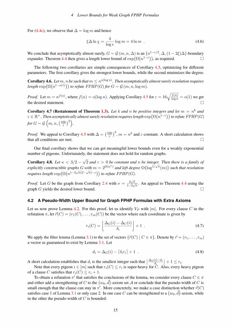
For (4.4c), we observe that ∆ = logm and hence

ξ∆ lnχ =4

log elogm = 4 lnm . (4.6)

We conclude that asymptotically almost surely, G ∼ G (m,n,∆) is an(n1−ε/2,∆, (1− 2ξ)∆

)-boundary

expander. Theorem 4.4 then gives a length lower bound of exp(Ω(n1−ε)), as required.

The following two corollaries are simple consequences of Corollary 4.5, optimizing for differentparameters. The first corollary gives the strongest lower bounds, while the second minimizes the degree.

Corollary 4.6. Letm,n be such thatm ≤ no(logn). Then asymptotically almost surely resolution requireslength exp

(Ω(n1−o(1)

))to refute FPHP(G) for G ∼ G (m,n, logm).

Proof. Let m = nf(n), where f(n) = o(logn). Applying Corollary 4.5 for ε = 16√

f(n)logn = o(1) we get

the desired statement.

Corollary 4.7 (Restatement of Theorem 1.3). Let k and n be positive integers and let m = nk andε ∈ R+. Then asymptotically almost surely resolution requires length exp

(Ω(n1−ε)) to refuteFPHP(G)

for G ∼ G(m,n,

(16kε

)2).

Proof. We appeal to Corollary 4.5 with ∆ =(

16kε

)2, m = nk and ε constant. A short calculation showsthat all conditions are met.

Our final corollary shows that we can get meaningful lower bounds even for a weakly exponentialnumber of pigeons. Unfortunately, the statement does not hold for random graphs.

Corollary 4.8. Let κ < 3/2 −√

2 and ε > 0 be constant and n be integer. Then there is a family ofexplicitly constructible graphs G with m = 2Ω(nκ) and left degree O

(log1/

√κ(m)

)such that resolution

requires length exp(Ω(n1−2

√κ(2−

√κ)−ε)) to refute FPHP(G).

Proof. Let G be the graph from Corollary 2.4 with ν = 2√κ

1−2√κ. An appeal to Theorem 4.4 using the

graph G yields the desired lower bound.

4.2 A Pseudo-Width Upper Bound for Graph FPHP Formulas with Extra Axioms

Let us now prove Lemma 4.2. For this proof, let us identify VP with [m]. For every clause C in therefutation π, let ~r(C) = (r1(C), . . . , rm(C)) be the vector where each coordinate is given by

ri(C) =

⌊∆G(i)−∆C(i)

δi

⌋+ 1 . (4.7)

We apply the filter lemma (Lemma 3.1) to the set of vectors ~r(C) | C ∈ π. Denote by ~r = (r1, . . . , rm)a vector as guaranteed to exist by Lemma 3.1. Let

di = ∆G(i)− dδirie+ 1 . (4.8)

A short calculation establishes that di is the smallest integer such that⌊∆G(i)−di

δi

⌋+ 1 ≤ ri.

Note that every pigeon i ∈ [m] such that ri(C) ≤ ri is super-heavy for C. Also, every heavy pigeonof a clause C satisfies that ri(C) ≤ ri + 1.

To obtain a refutation π′ that satisfies the conclusions of the lemma, we consider every clause C ∈ πand either add a strengthening of C to the

(w0, ~d

)-axiom set A or conclude that the pseudo-width of C is

small enough that the clause can stay in π′. More concretely, we make a case distinction whether ~r(C)satisfies case 1 of Lemma 3.1 or only case 2. In one case C can be strengthened to a

(w0, ~d

)-axiom, while

in the other the pseudo-width of C is bounded:

15


1. C satisfies∣∣i ∈ [m] | ri(C) ≤ ri

∣∣ ≥ w0: As every pigeon i ∈ [m] with ri(C) ≤ ri also satisfies∆C(i) ≥ di, we can strengthen this clause to a

(w0, ~d

)-axiom and add it to A. This reduces the

pseudo-width of this clause to w0.

2. C satisfies∣∣i ∈ [m] | ri(C) ≤ ri + 1

∣∣ ≤ O(α · w0): As every heavy pigeon always satisfiesri(C) ≤ ri + 1, the pseudo-width of C is O(α · w0).

This concludes the proof as |A| ≤ L(π) and the pseudo-width of π′ is O(α · w0) by construction.

4.3 A Pseudo-Width Lower Bound for Graph FPHP Formulas with Extra Axioms

We continue to the proof of Lemma 4.3. Using Definition 3.2, we define the set of relevant pigeons of aclause C as

closure(C) = closurer,(1−3ξ)∆(P~d,~δ(C)) , (4.9)

where P~d,~δ(C) denotes the set of (~d, ~δ)-heavy pigeons for C as defined in Definition 4.1. By definition,the closure of a set T contains T itself but is only defined if |T | ≤ r. However, if

∣∣P~d,~δ(C)∣∣ ≥ r ≥ rξ/4

then we already have the lower bound claimed in the lemma, and so we may assume that the closure iswell defined for all clauses in the refutation π. This implies, in particular, that for every clause C ∈ π wehave P~d,~δ(C) ⊆ closure(C).

Let us next construct the linear space Λ and describe how matchings are mapped into it. Fix a field F ofcharacteristic 0 and for each pigeon i ∈ VP let Λi be a linear space over F of dimension ∆G(i)−di+ δi/4.Let Λ be the tensor product Λ =

⊗i∈VP Λi and denote by λi : VH 7→ Λi a function with the property that

any subset of holes J ⊆ VH of size at least dim(Λi) spans Λi. In other words, for J as above we have thatΛi = span(λi(j) : j ∈ J). This is how we will realize the idea of “lossy counting.” For J ⊆ VH suchthat |J | ≤ dim(Λi) we have exact counting dim(span(λi(j) | j ∈ J)) = |J |, but when |J | > dim(Λi)gets large enough we have dim(span(λi(j) | j ∈ J)) = dim(Λi).

In order to map functions VP 7→ VH into Λ, we define λ : V VPH 7→ Λ by λ(j1, . . . , jm) =⊗

i∈VP λi(ji), where will we abuse notions slightly in that we identify a vector with the 1-dimensionalspace spanned by this vector. For a partial function ϕ : VP 7→ VH , we let λ(ϕ) be the span of all totalextensions of ϕ (not necessarily matchings), or equivalently

λ(ϕ) =⊗

i∈dom(ϕ)

λi(ϕi)⊗⊗

i 6∈dom(ϕ)

Λi . (4.10)

Recall thatM is the set of all partial matchings on the graphG and that we interchangeably think of partialmatchings as partial functions ϕ : VP → VH or as Boolean assignments ρϕ as defined in (2.3). For eachclause C, we are interested in the partial matchings ϕ ∈M with domain dom(ϕ) = closure(C) such thatρϕ does not satisfy C. We refer to the set of such matchings as the zero space of C and denote it by

Z(C) = ϕ ∈M | dom(ϕ) = closure(C) ∧ ρϕ(C) 6= 1 . (4.11)

We associate C with the linear space

λ(C) = span(λ(ϕ) | ϕ ∈ Z(C)) . (4.12)

Note that contradiction is mapped to Λ, i.e., λ(⊥) = Λ.We assert that the span of the axioms span(λ(A) | A ∈ FPHP(G)∪A) is a proper subspace of Λ.

Lemma 4.9. If |A| ≤ (1 + ξ)w0 , then span(λ(A) | A ∈ FPHP(G) ∪ A) ( Λ.

Accepting this claim without proof for now, this implies that in π there is some resolution step derivingC from C0 and C1 where the subspace of the resolvent is not contained in the span of the subspaces ofthe premises, or in other words λ(C) * span(λ(C0), λ(C1)). Our next lemma, which is the heart of theargument, says that this cannot happen as long as the closures of the clauses are small.

16


closure(C)

closure(C1)

closure(C0)

Ddom(ϕ′)

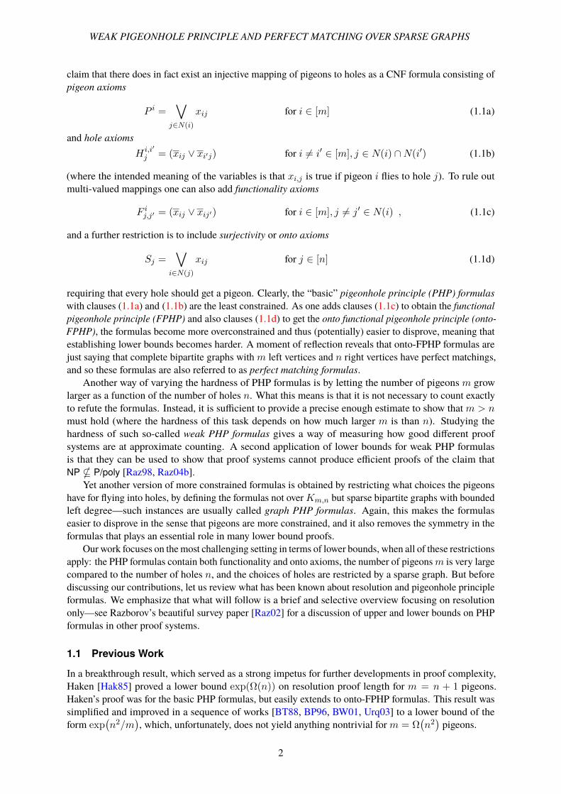
Figure 1: Depiction of relations between closure(C), closure(Ci), i = 1, 2,dom(ϕ′) andD in proof of Lemma 4.10.

Lemma 4.10. Let C be derived from C0 and C1. If max|closure(C0)|, |closure(C1)|, |closure(C)| ≤r/4, then λ(C) ⊆ span(λ(C0), λ(C1)).

Since contradiction cannot be derived while the closure is of size at most r/4, any refutation π mustcontain a clause C with |closure(C)| > r/4. But then Lemma 3.3 implies that C has pseudo-width atleast rξ/4, and Lemma 4.3 follows. All that remains for us is to establish Lemmas 4.9 and 4.10.

Proof of Lemma 4.9. We need to show that the axioms FPHP(G) ∪ A do not span all of Λ. We startwith the axioms in FPHP(G).

Let A be pigeon axiom P i as in (1.1a) or a functionality axiom F ij,j′ as in (1.1c). Note that i is a heavypigeon forA. Clearly, there are no pigeon-to-hole assignments for pigeon i that do not satisfyA. Thus thereare no matchings on closure(A) that do not satisfy A. We conclude that λ(A) = ∅. If instead A is a holeaxiom H i,i′

j as in (1.1b), then we can observe that ∆G(i)− 1 ≥ di − δi since δi = 4ξ∆G(i) ≥ 2ξ∆ ≥ 1(by boundary expansion). This implies that A has two heavy pigeons. Observe that there are no matchingson these two pigeons that do not satisfy A. Thus Z(A) = ∅ and we conclude that λ(A) = ∅.

Now consider the(w0, ~d

)-axioms in A. We wish to show that any A ∈ A can only span a very small

fraction of Λ. We can estimate the the number of dimensions λ(A) spans by

dimλ(A) ≤∏

i/∈P~d(A)

dim Λi ·∏

i∈P~d(A)

(∆G(i)− di) . (4.13)

Hence the fraction of the space Λ that A may span is bounded by

dimλ(A)

dim Λ≤

∏i∈P~d(A)

∆G(i)− di∆G(i)− di + δi/4

≤ (1− ξ)w0 . (4.14)

As |A| ≤ (1 + ξ)w0 we can conclude that not all of Λ is spanned by the axioms.

Proof of Lemma 4.10. For conciseness of notation, let us write S01 = closure(C0) ∪ closure(C1) andS = closure(C). In order to establish the lemma, we need to show for all ϕ ∈ Z(C) that

λ(ϕ) ⊆ span(λ(C0), λ(C1)) . (4.15)

To comprehend the argument that will follow below, it might be helpful to refer to the illustration inFigure 1.

Denote by ϕ′ the restriction of ϕ to the domain S ∩ S01 and note that C is not satisfied under ρϕ′ .Also, observe that if a matching η extends a matching η′, then λ(η) is contained in λ(η′). This is so since

17


for any pigeon i ∈ dom(η) \ dom(η′) we have from (4.10) that η′ picks up the whole subspace Λi whileη only gets a single vector. Thus, if we can show that λ(ϕ′) ⊆ span(λ(C0), λ(C1)), then we are done asϕ extends ϕ′ and hence λ(ϕ) ⊆ λ(ϕ′).

Let D = S01 \ S and denote byMD the set of matchings that extend ϕ′ to the domain D and donot satisfy C. Since each matching ψ ∈ MD fails to satisfy C, by the soundness of the resolution rulewe have that it also fails to satisfy either C0 or C1. Assume without loss of generality that ψ does notsatisfy C0 and denote by ψ′ the restriction of ψ to the domain of closure(C0). From (4.11) we see thatψ′ ∈ Z(C0) and therefore λ(ψ) ⊆ λ(ψ′) ⊆ λ(C0).

So far we have argued that for all matchings ψ ∈MD it holds that λ(ψ) ⊆ span(λ(C0), λ(C1)). Letλ(MD) = span(λ(ψ) | ψ ∈ MD). If we can show that the set of matchingsMD is large enough forλ(MD) = λ(ϕ′) to hold, then the lemma follows. In other words, we want to show that λ(MD) projectedto ΛD =

⊗i∈D Λi spans all of the space ΛD .

To argue this, note first that D is completely outside the closure(C). Furthermore, by assumption wehave |closure(C)| ≤ r/4 and |D| ≤ |S01| ≤ r/2. An application of Lemma 3.4 now tells us that

|∂G\(closure(C)∪N(closure(C)))(D)| ≥ (1− 3ξ)∆|D| . (4.16)

By an averaging argument, there must exist a pigeon i1 ∈ D that has more than (1 − 3ξ)∆ uniqueneighbours in ∂G\(closure(C)∪N(closure(C)))(D). The same argument applied to D \ i1 show that somepigeon i2 has more than (1− 3ξ)∆ unique neighbours on top of the neighbours reserved for pigeon i1.Iterating this argument, we derive by induction that for each pigeon i ∈ D we can find (1− 3ξ)∆ distinctholes in N(D). Since all pigeons in D are light in C, it follows that at most di − δi mappings of pigeon ican satisfy the clause C. Hence, there are at least

(1− 3ξ)∆− (di − δi) ≥ (1− 3ξ)∆G(i)− di + 4ξ∆G(i) ≥ ∆G(i)− di + δi/4 (4.17)

many holes to which each pigeon in D can be sent, independently of all other pigeons in D, withoutsatisfying C. As we have that dim(Λi) = ∆G(i)− di + δi/4, we conclude that λ(MD) projected to ΛDspans the whole space. This concludes the proof of the lemma.

5 Lower Bounds for Perfect Matching Principle Formulas

In this section, we show that the perfect matching principle formulas defined over even highly unbalancedbipartite graphs require exponentially long resolution refutations if the graphs are expanding enough.

Just as in [Raz04b], our proof is by an indirect reduction to the FPHP lower bound, and therefore thereis a significant overlap in concepts and notation with Section 4. However, since there are also quite afew subtle shifts in meaning, we restate all definitions in full below to make the exposition in this sectionself-contained and unambiguous.

We first review some useful notions from [Raz01]. Let G = (V,E) denote the graph over which theformulas are defined. For a clause C and a vertex v ∈ V (G), let the clause-neighbourhood of v in C,denoted by NC(v), be the vertices u ∈ V (G) with the property that C is satisfied if v is matched to u,that is,

NC(v) = u ∈ V | e = u, v ∈ E and ρe(C) = 1 . (5.1)

For a set V ⊆ V (G) let NC(V ) be the union of the clause-neighbourhoods of the vertices in V , i.e.,NC(V ) =

⋃v∈V NC(v) and let the vth vertex degree of C be

∆C(v) = |NC(v)| . (5.2)

We think of a vertex v with large degree ∆C(v) as a vertex on which the derivation has not made anyprogress up to the point of deriving C, since the clause rules out very few neighbours. The vertices withhigh enough vertex degree in a clause are the heavy vertices of the clause as defined next.

18


Definition 5.1 (Vertex weight, pseudo-width and(w0, ~d

)-axioms). Let ~d = (d1, . . . , dm+n) and ~δ =

(δ1, . . . , δm+n) be two vectors such that ~d is elementwise greater than ~δ. We say that a vertex v is ~d-super-heavy for C if ∆C(v) ≥ dv and that vertex v is (~d, ~δ)-heavy for C if ∆C(v) ≥ dv − δv. When ~d and ~δ areunderstood from context we omit the parameters and just refer to super-heavy and heavy vertices. Verticesthat are not heavy are referred to as light vertices. The set of vertices that are super-heavy for C is denotedby

V~d(C) = v ∈ V | ∆C(v) ≥ dv (5.3)

and the set of heavy vertices for C is denoted by

V~d,~δ(C) = v ∈ V | ∆C(v) ≥ dv − δv . (5.4)

The pseudo-width w~d,~δ(C) = |V~d,~δ(C)| of a clause C is the number of heavy vertices in it, and thepseudo-width of a resolution refutation π is w~d,~δ(π) = maxC∈π w~d,~δ(C). We refer to clauses C withprecisely w0 super-heavy vertices as

(w0, ~d

)-axioms.

To a large extent, the proof of the lower bounds for perfect matching formulas follows the general ideaof the proof of Theorem 4.4: given a short refutation we first apply the filter lemma to obtain a refutationof small pseudo-width; we then prove that in small pseudo-width contradiction cannot be derived and canthus conclude that no short refutation exists. In more detail, given a short resolution refutation π, we usethe filter lemma (Lemma 3.1) to get a filter vector ~d = (d1, . . . , dm+n) such that each clause either hasmany super-heavy vertices or not too many heavy vertices (for an appropriately chosen vector ~δ). Clearly,clauses that fall into the second case of the filter lemma have bounded pseudo-width. Clauses in the firstcase, however, may have very large pseudo-width. In order to obtain a proof of low pseudo-width, theselatter clauses are strengthened to

(w0, ~d

)-axioms and added to a special setA. This then gives a refutation

π′ that refutes the formula PM (G) ∪ A in bounded pseudo-width as stated in the next lemma.

Lemma 5.2. Let G = (VL.∪ VR, E) be a bipartite graph with |VL| = m and |VR| = n; let π be a res-

olution refutation of PM (G); let w0, α ∈ [m + n] be such that w0 > logL(π) and w0 ≥ α2 ≥ 4,and let ~δ = (δ1, . . . , δm+n) be defined by δv = ∆G(v) logα

log(m+n) for v ∈ V (G). Then there exists an

integer vector ~d = (d1, . . . , dm+n), with δv < dv ≤ ∆G(v) for all v ∈ V (G), a set of(w0, ~d

)-

axioms A with |A| ≤ L(π), and a resolution refutation π′ of PM (G) ∪ A such that L(π′) ≤ L(π) andw~d,~δ(π

′) ≤ O(α · w0).

The proof of the above lemma is omitted as it is syntactically equivalent to the proof of Lemma 4.2.Until this point, we have almost mimicked the proof of Theorem 4.4. The main differences will appear inthe proof of the counterpart to Lemma 5.2, which states a pseudo-width lower bound.

Lemma 5.3. Assume for ξ ≤ 1/64 and m,n, r,∆ ∈ N that G = (VL.∪ VR, E) is an (r,∆, (1− 2ξ) ∆)-

boundary expander with |VL| = m, |VR| = n, ∆ ≥ logm/ξ2, and min∆G(v) : v ∈ VR ≥ r/ξ. Let~δ = (δv | v ∈ V (G)) be defined by δv = 64∆G(v)ξ and suppose that ~d = (dv | v ∈ V (G)) is an integervector such that δv < dv ≤ ∆G(v) for all v ∈ V (G). Fix w0 such that 64 ≤ w0 ≤ rξ − log n and let Abe an arbitrary set of

(w0, ~d

)-axioms with |A| ≤ (1 + 16ξ)w0/8. Then every resolution refutation π of

PM (G) ∪ A has either length L(π) ≥ 2w0/32 or pseudo-width w~d,~δ(π) ≥ rξ.

The proof of the above lemma is based on a sort of reduction to the FPHP(G) case. The idea, dueto Razborov [Raz04b], is to first pick a partition of the vertices of G that looks random to every clausein the refutation and then simulate the FPHP(G) lower bound on this partition. In our setting, however,this process gets quite involved. Already implementing the partition idea of Razborov is non-trivial: for afixed clause C some vertices that are light may be super-heavy with respect to the partition, and we do nothave an upper bound on the pseudo-width any longer. The insight needed to solve this issue is to show thatby expansion there are not too many such vertices per clause, and then adapt the closure definition to takethese vertices into account.

19


Another issue we run into is that the span argument from Section 4 cannot be applied to all thevertices in the graph. Instead, for the vertices in VR, we need to resort to the span argument from [Raz03].Moreover, vertices in the neighbourhood of D (as defined in the proof of Lemma 4.10) may already bematched and we are hence unable to attain enough matchings. Our solution is to consider a “lazy” edgeremoval procedure from the original matching, which with a careful analysis can be shown to circumventthe problem—see Section 5.3 for details.

5.1 Formal Statements of Perfect Matching Formula Lower Bounds

Let us state our lower bounds for the perfect matching formulas and defer the proof of Lemma 5.3 toSection 5.3.

Theorem 5.4. Let G = (U.∪ V,E) be a bipartite graph with m = |U | and n = |V |. Suppose that G

is an (r,∆, (1− 2ξ) ∆)-boundary expander for ∆ ≥ log(m+n)ξ2

and ξ = logα64 log(m+n) where α ≥ 2 and

α3

logα = o(

rlog(m+n)

), which furthermore satisfies the degree requirement min∆G(v) : v ∈ V ≥ r/ξ.

Then resolution requires length exp(

Ω(

r log2 αα log2(m+n)

))to refute the perfect matching formula PM (G)

defined over G.

We remark that this theorem also holds if we replace the minimum degree constraint of V with anexpansion guarantee from V to U . We state the theorem in the above form as we want to apply it to thegraphs from [GUV09] for which we have no expansion guarantee from V to U .

Proof of Theorem 5.4. Let w0 = ε0rξα , for some small enough ε0 > 0 . Suppose for the sake of contradic-

tion that π is a resolution refutation of PM (G) such that L(π) < (1 + 16ξ)w0/8. Since w0 > logL(π),by Lemma 5.2 we have that there exists an integer vector ~d = (d1, . . . , dm+n), with δv < dv ≤ ∆G(v),a set of

(w0, ~d

)-axioms A with |A| ≤ L(π) < (1 + 16ξ)w0/8, and a resolution refutation π′ of

PM (G) ∪ A such that L(π′) ≤ L(π) and w~d,~δ(π′) ≤ Kαw0 for some large enough constant K. Since

L(π′) < (1 + 16ξ)w0/8 ≤ 2w0/32, by Lemma 5.3, we have that w~d,~δ(π′) ≥ rξ ≥ αw0/ε0. Choosing

ε0 < 1/K, we get a contradiction and, thus, L(π) ≥ (1 + 16ξ)w0/8 = exp(

Ω(rξ2

α

)).

As in Section 4, we have a general statement for random graphs.

Corollary 5.5. Let m and n be positive integers, let ∆ : N+ → N+ and ε : N+ → [0, 1] be any

monotone functions of n such that n3 < m ≤ n(ε/128)2 logn and n ≥ ∆ ≥ log(m+ n)(

128 log(m+n)ε logn

)2.

Then asymptotically almost surely resolution requires length exp(Ω(n1−ε)) to refute PM (G) for G ∼

G(m,n,∆

).

Proof. For simplicity, let us assume that m+ = n(ε/128)2 logn and ∆− = log(m + n) ·((128 log(m +

n))/(ε log n))2 are integers. It suffices to prove the claim for m = m+ and ∆ = ∆−. Indeed, if

G ∼ G (m,n,∆), for ∆ > ∆−, we can sample a random subgraph G′ ∼ G(m,n,∆−

)of G by choosing

a random subset of appropriate size of each neighbourhood of a left vertex and applying a restrictionzeroing out the other edges. Furthermore, as for smaller m the formula gets less constrained and hence thelower bound is easier to obtain, it suffices to prove it for m = m+.

We want to apply Lemma 2.2 for χ = α = nε/4 and ξ = logα64 logm , and towards this end we argue that

the inequalities

ξ < 1/2 , (5.5a)ξ lnχ ≥ 2 , (5.5b)

ξ∆ lnχ ≥ 4 lnm (5.5c)

20


all hold. First observe that ξ = 32ε logn and n < n(ε/128)2 logn, from which we conclude that 1

logn <(ε

128

)2.Hence, the first inequality (5.5a) holds for n large enough. A simple calculation

ξ lnχ =32

ε log n

ε lnn

4≥ 2 (5.6)

shows that (5.5b) is also true. Finally, for (5.5c), we observe that ∆ ≥ log2m and hence

ξ∆ lnχ ≥ 8

log elog2m ≥ 4 lnm . (5.7)

We conclude that asymptotically almost surely G ∼ G (m,n,∆) is an(n1−ε/2,∆, (1− 2ξ)∆

)-boundary

expander. Furthermore, by the Chernoff inequality asymptotically almost surely all right vertices havedegree at least n · 64 log(m+n)

ε logn . Thus, Theorem 5.4 gives a length lower bound of exp(Ω(n1−ε)) as

claimed.

The following corollary is a simple consequence of Corollary 5.5, optimizing for the strongest lowerbounds.

Corollary 5.6 (Restatement of Theorem 1.1). Letm,n be such thatm ≤ no(logn). Then asymptoticallyalmost surely resolution requires length exp

(Ω(n1−o(1)

))to refute PM (G) forG ∼ G

(m,n, 8 log2m

).

Proof. Let m = nf(n), where f(n) = o(log n). Applying Corollary 5.5 for ε = 128√

f(n)logn = o(1), we

get the desired statement.

Our final corollary shows that we even get meaningful lower bounds for highly unbalanced bipartitegraphs. As was the case for FPHP(G), the required expansion is too strong to hold for random graphswith such large imbalance, but does hold for explicitly constructed graphs from [GUV09].

Corollary 5.7 (Restatement of Theorem 1.2). Let κ < 3/2−√

2 and ε > 0 be constants, and let n bean integer. Then there is a family of (explicitly constructible) graphs G with m = 2Ω(nκ) and left degreeO(log1/

√κ(m)), such that resolution requires length exp(Ω(n1−2

√κ(2−

√κ)−ε)) to refute PM (G).

Proof. Let G be the graph from Corollary 2.4 with ν = 2√κ

1−2√κ

. In order to apply Theorem 5.4 we need tosatisfy the minimum right degree constraint. A simple way of doing this is by adding n2 edges to G suchthat each vertex on the right has exactly n incident edges added while each vertex on the left has at mostone incident edge added. This will leave us with a graph which has large enough right degree while eachleft degree increased by at most one. The additional edges may reduce the boundary expansion a bit, buta short calculation shows that by choosing ξ = logα

128 log(m+n) in Corollary 2.4, we can still guarantee theneeded boundary expansion for Theorem 5.4. The corollary bound follows.

5.2 Defining Pigeons and Holes

As stated earlier, we prove the PM (G) lower bound by simulating the FPHP(G) lower bound fromSection 4 on a partition VP

.∪ VH of the vertices of G. As the notation suggests, we think of the vertices in

VP as pigeons and of the vertices in VH as holes.Let us first motivate the properties—captured in Lemma 5.8—that such a partition must satisfy in

order for the FPHP(G) simulation to go through. To begin with, recall that in the proof of Lemma 4.9 weshow that a

(w0, ~d

)-axiom only spans an exponentially small fraction of the linear space Λ. The argument

crucially relies on the fact that there are many super-heavy pigeons in every(w0, ~d

)-axiom. To make this

work over the partition VP.∪ VH , we require that a constant fraction of the super-heavy vertices of every(

w0, ~d)-axiom are in VP and that super-heavy vertices remain super-heavy with respect to this partition.

This first issue is addressed by property 1 of Lemma 5.8 whereas the second issue is guaranteed by theother properties: property 2 ensures that for every vertex roughly half of its neighbours are in VH while

21


properties 3 and 4 ensure that most clause-neighbourhoods behave in the same manner, i.e., up to a smallset of vertices per clause every clause-neighbourhood of a vertex has roughly half of its vertices in VH .Combining these arguments, we can bound the fraction of the space spanned by a

(w0, ~d

)-axiom.

The other main technical step of the FPHP(G) lower bounds is Lemma 4.10 which state that in lowpseudo-width the linear space associated with a resolvent never leaves the span of the premises. Thisargument relies on the expansion guarantee of the underlying graph and the fact that light pigeons areunconstrained. The required graph expansion (see Lemma 5.10) will follow from property 2 and properties2–4 are used to argue that light pigeons are also unconstrained with repect to the partition.

Lemma 5.8. Let G = (VL.∪ VR, E) be an (r,∆, (1− 2ξ) ∆)-boundary expander for ξ ≤ 1/4 and

|VL| ≥ 4. Fix w0 such that 64 ≤ w0 ≤ r and letA be a set of(w0, ~d

)-axioms of size |A| ≤ exp(w0/32).

Moreover, suppose that ∆ ≥ log|VL|/ξ2 and min∆G(v) : v ∈ VR ≥ (log|VR| + w0)/ξ2. If π isa resolution refutation of PM (G) ∪ A with L(π) ≤ exp(w0/32), then there exists a vertex partitionV(G) = VP ∪VH such that

1. for every A ∈ A:

|V~d(A) ∩ VP | ≥ w0/4 ,

2. for every v ∈ V: ∣∣|NG(v) ∩ VH | − 1/2|NG(v)|∣∣ ≤ 4ξ

∣∣NG(v)∣∣ ,

3. for every C ∈ π and for every v ∈ VR:∣∣|NC(v) ∩ VH | − 1/2|NC(v)|∣∣ ≤ 4ξ|NG(v)| ,

4. for every C ∈ π there is a set of vertices V (C) ⊆ VL, with |V (C)| ≤ w0/8, such that for everyv ∈ VL \ V (C): ∣∣|NC(v) ∩ VH | − 1/2|NC(v)|

∣∣ ≤ 4ξ∆ .

The analogue of above lemma in [Raz04b] is Claim 19. The main difference is that in our settingproperty 4 does not always hold for all vertices in the graph while in Razborov’s setting the correspondingproperty always holds.

In order to argue that this error set V (C) is small, we need G to be a good expander. To this end weuse the following claim which states that if for a fixed clause C there are many vertices v ∈ VL such that|NC(v) ∩ VH | does not behave as expected, then, by expansion, we can find a large set of vertices V ?(C)whose clause-neighbourhood in VH (i.e., the set NC(V ?(C)) ∩ VH ) deviates from its expected size.

Claim 5.9. Let G = (VL.∪ VR, E) be an (r,∆, (1− 2ξ) ∆)-boundary expander. Fix any partition

V (G) = VP.∪ VH and any clause C. Let

V (C) = v ∈ VL :∣∣|NC(v) ∩ VH | − 1/2|NC(v)|

∣∣ > 4ξ∆ .

If |V (C)| > w0/8, then there is a set of vertices V ?(C) ⊆ V (C), with |V ?(C)| = w0/16, such that∣∣|NC(V ?(C)) ∩ VH | − 1/2|NC(V ?(C))|∣∣ > 2ξ∆|V ?(C)| .

Proof. Denote by V +(C) (V −(C) respectively) the vertices in V (C) that have more neighbours (lessneighbours respectively) in VH than the expected 1/2

∣∣NC(v)∣∣. As |V (C)| > w0/8, one of the sets V +(C)

or V −(C) is of cardinality at least w0/16.

22


Case 1: Suppose V +(C) ≥ w0/16 and let V ?(C) be any subset of V +(C) of size w0/16. Asboundary expansion of G guarantees that V ?(C) has at most 2ξ∆|V ?(C)| edges to non-uniqueneighbours in G we derive

|NC(V ?(C)) ∩ VH | ≥∑

v∈V ?(C)

|NC(v) ∩ ∂(V ?(C)) ∩ VH | (5.8)

≥∑

v∈V ?(C)

|NC(v) ∩ VH | − 2ξ∆|V ?(C)| (5.9)

>∑

v∈V ?(C)

(1/2|NC(v)|+ 4ξ∆

)− 2ξ∆|V ?(C)| (5.10)

≥ 1/2|NC(V ?(C))|+ 2ξ∆|V ?(C)| , (5.11)

where the strict inequality follows by definition of V +(C).

Case 2: Suppose V −(C) ≥ w0/16 and let V ?(C) be any subset of V −(C) of size w0/16. Similarto the previous case we can conclude that

|NC(V ?(C)) ∩ VH | ≤∑

v∈V ?(C)

|NC(v) ∩ VH | (5.12)

<∑

v∈V ?(C)

(1/2|NC(v)| − 4ξ∆

)(5.13)

≤ 1/2|NC(V ?(C))| − 2ξ∆|V ?(C)| , (5.14)

where the last inequality uses that V ?(C) has at most 2ξ∆|V ?(C)| edges incident to non-uniqueneighbours in G.

Combining both cases yields the claim.

Proof of Lemma 5.8. Pick a partition V = VP.∪VH uniformly at random. In what follows we show that

property 1 holds with probability at least 3/4 and properties 2, 3 and 4 each hold with probability at least7/8. Hence there exists a partition that satisfies all four properties simultaneously.

For the first property, since E[|V~d(A) ∩VP|

]= w0/2, by the multiplicative Chernoff bound we have

that

Pr[|V~d(A) ∩VP| ≤ w0/4

]≤ exp (−w0/16) . (5.15)

Since |A| ≤ exp(w0/32) and w0 ≥ 64, a union bound over A gives us that property 1 holds except withprobability exp(−w0/32) ≤ 1/4.

To analyse properties 2 and 3, let C either be a clause in π or be the graph G (i.e., the clause thatcontains all variables) and fix an arbitrary v ∈ V (G). By Chernoff bound (Theorem 2.1) we get that

Pr[∣∣|NC(v) ∩VH| − 1/2|NC(v)|

∣∣ ≥ 4ξ|NG(v)|]≤ 2 exp

(− (4ξ|NG(v)|)2

|NC(v)|+ 4ξ|NG(v)|

)(5.16)

≤ exp(−8ξ2|NG(v)|+ 1

), (5.17)

where the last inequality holds as |NC(v)| ≤ |NG(v)| and ξ ≤ 1/4.By a union bound argument over the clauses in π and v ∈ VR, we have that Property 3 holds except

with probability 1/8. For property 2, we need to analyse vertices in VL and in VR separately. On theone hand, since min∆G(v) : v ∈ VL ≥ (1 − 2ξ)∆ ≥ log|VL|

2ξ2and |VL| ≥ 4, a union bound over

v ∈ VL shows that property 2 holds for all vertices VL except with probability 1/16. On the other, as

23


min∆G(v) : v ∈ VR ≥ (log|VR|+ w0)/ξ2, a union bound yields that property 2 holds for all v ∈ VRexcept with probability 1/16.

To obtain property 4, fix a clause C and consider the set V(C) that contains all vertices v ∈ VLsatisfying ∣∣|NC(v) ∩VH| − 1/2|NC(v)|

∣∣ > 4ξ∆ . (5.18)

We want to show that it is unlikely that |V(C)| ≥ w0/8. Note that such a large V(C) implies by Claim 5.9that there is a set S ⊆ VL of size w0/16 such that

∣∣|NC(S)∩VH| − 1/2|NC(S)|∣∣ ≥ 2ξ∆|S|. By a union

bound over all such sets S and applying Chernoff bound (Theorem 2.1) we have that

Pr[|V(C)| ≥ w0/8

]≤(|VL|w0/16

)maxS⊆VL:|S|=w0/16

Pr[∣∣|NC(S) ∩VH| − 1/2|NC(S)|

∣∣ ≥ ξ∆w0/8]

(5.19)

≤ |VL|w0/16 · 2 exp

(− (ξ∆w0/8)2

∆w0/16 + ξ∆w0/8

)(5.20)

≤ exp(−ξ2∆w0/8 + 1 + log|VL| · w0/16

)(5.21)

≤ exp (− log|VL| · w0/16 + 1) , (5.22)

where for (5.20) we observe that |NC(S)| ≤ ∆|S|, for (5.21) we need that ξ ≤ 1/4 and for (5.22)that ∆ ≥ log|VL|/ξ2. By a union bound over all clauses in π we see that property 4 holds except withprobability 1/8.

Let VP.∪ VH be a partition of V(G) as guaranteed to exist by Lemma 5.8. For an overview of the

vertex sets and how they relate we refer to Figure 2. The following lemma shows that the vertices in VLexpand into the set VR ∩ VH . Let G′ = G \ (VR ∩ VP ) with vertex partition (VL

.∪ (VR \ VP )).

Lemma 5.10. The graph G′ is an (r, (1 + 8ξ)∆/2, (1− 12ξ)∆/2)-boundary expander.

Proof. By Lemma 5.8, property 2, every vertex in VP ∩ VL has degree at most (1 + 8ξ)NG(v)/2 and atleast (1− 8ξ)NG(v)/2. By the expansion guarantee ofG, we know that |NG(v)| ≥ (1− 2ξ)∆. Thereforeall sets of size 1 are good enough boundary expanders. We continue by induction on the size of the set. LetS be a set of vertices of size at most r. In the original graph G, this set S has at least (1− 2ξ)∆|S| manyunique neighbours. Thus there is a vertex v in S that has at least (1− 2ξ)∆ many unique neighbours in G.Further, by Lemma 5.8, property 2, the vertex v has at least (1− 8ξ)∆/2 many neighbours in VR ∩ VH .Hence v has at least (1 − 12ξ)∆/2 many unique neighbours in VH . From the induction hypothesis onS \ v, it follows that S has the required number of unique neighbours in VH .

5.3 Pseudo-Width Lower Bound

We start by setting up the notation we will need to prove Lemma 5.3.Let C be a clause in π, let V (C) = v ∈ VL :

∣∣|NC(v) ∩ VH | − 1/2|NC(v)|∣∣ > 4ξ∆ and

V (C) = (V~d,~δ(C) ∩ VL) ∪ V (C). The closure of C is a subset of VL in the graph G′, defined by

closure(C) = closurer,(1−20ξ)∆/2(V (C)) . (5.23)

We define the closure only on VL as we only have an expansion guarantee from VL into VR ∩ VH . As theconcept of closure only makes sense on vertex sets which are expanding, we do not define it on VR. Theset of relevant vertices of a clause C are the vertices in closure(C)∪ V~d,~δ(C). With this definition at handwe proceed to set up the linear spaces that realize the lossy counting (see Section 4). Let us stress the factthat only vertices in VP are associated with a linear space.

Fix a field F of characteristic 0 and for each vertex v ∈ VP let Λv be a linear space over F of dimension1/2(∆G(v)− dv + δv/2). Let Λ =

⊗v∈VP Λv and denote by λv : VH 7→ Λv a function with the property

that any image of a subset S ⊆ VH of size |S| ≥ dim(Λv) spans Λv, i.e., span(λv(u) : u ∈ S) = Λv.

24


LetM be the set of partial matchings in G that contain no edges from VP × VP . To map partialmatchings ϕ ∈M into Λ, we define λ :M 7→ Λ by

λ(ϕ) =⊗

v∈V (ϕ)∩VP

λv(ϕv)⊗⊗

v∈VP \V (ϕ)

Λv . (5.24)

Recall that each partial matchingϕ ∈M has an associated partial boolean assignment ρϕ as defined in (2.3).For each clauseC, we are interested in the partial matchings ϕ ∈M that match all of closure(C)∪V~d,~δ(C)such that ρϕ does not satisfy C. We refer to the set of such matchings as the zero space of C and denote itby

Z(C) = ϕ ∈M | V (ϕ) ⊇ (closure(C) ∪ V~d,~δ(C)) ∧ C(ρϕ) 6= 1 . (5.25)

We associate C with the linear space

λ(C) = span(λ(ϕ) | ϕ ∈ Z(C)) . (5.26)

Note that contradiction is mapped to Λ, i.e., λ(⊥) = Λ.The following lemma asserts that the span of the axioms span(λ(A) | A ∈ PM (G) ∪ A) is a

proper subspace of Λ.

Lemma 5.11. If |A| ≤ (1 + 16ξ)w0/8, then span(λ(A) | A ∈ PM (G) ∪ A) ( Λ.

Deferring the proof of this lemma for now, note this implies that in the refutation π there is a resolutionstep deriving C from C0 and C1 where the subspace of the resolvent is not contained in the span of thesubspaces of the premises, or in other words λ(C) 6⊆ span(λ(C0), λ(C1)). The following lemma, whichis the heart of the argument, says that this cannot happen while the sets of relevant vertices of the clausesare small.

Lemma 5.12. Let C be derived from C0 and C1. If max|closure(C0) ∪ V~d,~δ(C0)|, |closure(C1) ∪V~d,~δ(C1)|, |closure(C) ∪ V~d,~δ(C)| ≤ r/4, then λ(C) ⊆ span(λ(C0), λ(C1)).

Deferring the proof of Lemma 5.12 to Section 5.4, we proceed to show how Lemma 5.3 follows fromwhat we have established so far.

Proof of Lemma 5.3. Lemma 5.11 and Lemma 5.12 imply that contradiction cannot be derived while theset of relevant vertices is of size at most r/4 and hence any refutation π must contain a clause C with|closure(C) ∪ V~d,~δ(C)| ≥ r/4. If for such a clauses C it holds that |V~d,~δ(C)| ≥ rξ, then Lemma 5.3follows. Otherwise, recall that closure(C) = closurer,ν(V (C)), for ν = (1− 20ξ)∆/2, and that G′ is an(r,∆′, c)-boundary expander by Lemma 5.10, where ∆′ = (1 + 8ξ)∆/2 and c = (1− 12ξ)∆/2. Thuswe can apply Lemma 3.3 to G′ and get that |V (C)| ≥ minr, (r/4− rξ) · (c− ν) /∆′ ≥ 3rξ/2. As bydefinition V (C) = (V~d,~δ(C)∩VL)∪ V (C) and by property 4 of Lemma 5.8 we have that |V (C)| ≤ w0/8,we conclude that

w~d,~δ(π) ≥ |V~d,~δ(C)| ≥ |V~d,~δ(C) ∩ VL| ≥ |V (C)| − |V (C)| ≥ 3rξ/2− w0/8 ≥ rξ . (5.27)

This completes the proof of Lemma 5.3.

Proof of Lemma 5.11. Suppose A is a vertex axiom P v or a functionality axiom F vw,w′ as in (1.1a) and(1.1c). Observe that v is a heavy vertex for A. Clearly, there are no matchings on v that do not satisfy A.We conclude that λ(A) = ∅.

Let us consider A ∈ A. These axioms may span a part of the space Λ but the fraction of the space Λthey span is sufficiently small. We first estimate the dimension of λ(A). By definition V (A) = v ∈ VL :∣∣|NA(v) ∩ VH | − 1/2|NA(v)|

∣∣ > 4ξ∆ and by property 4 of Lemma 5.8 it holds that |V (A)| ≤ w0/8.We partition VP into two sets U = VP \

(V~d,~δ(A) \ V (A)

)and W = VP ∩

(V~d,~δ(A) \ V (A)

). Note that

25


VL VR

VP

VH

Partition of V into VP and VH

DV (ϕ′)

Figure 2: Depiction of relations between VL, VR, VP , VH and the vertex sets in the proof of Lemma 5.12.

all vertices v ∈ W satisfy that∣∣|NA(v) ∩ VH | − 1/2|NA(v)|

∣∣ ≤ 4ξ∆. Using property 2 of Lemma 5.8we get that

dimλ(A) ≤∏v∈U

dim Λv ·∏v∈W

(|NG(v) ∩ VH | − |NA(v) ∩ VH |

)(5.28)

≤∏v∈U

dim Λv ·∏v∈W

(1/2|NG(v)|+ 4ξ|NG(v)| − 1/2|NA(v)|+ 4ξ|NG(v)|

)(5.29)

=∏v∈U

dim Λv ·∏v∈W

(1/2(|NG(v)| − |NA(v)|

)+ 8ξ|NG(v)|

)(5.30)

≤∏v∈U

dim Λv ·∏v∈W

(1/2(∆G(v)− dv) + δv/8

)(5.31)

≤∏v∈U

dim Λv ·∏v∈W

(dim Λv − δv/8

), (5.32)

where the second to last inequality follows from the fact that δv = 64ξ|NG(v)| and the last inequality fromthe definition of dim Λv.

Note that by property 1 of Lemma 5.8, |VP ∩ V~d,~δ(A)| ≥ w0/4 and hence |W | ≥ w0/8. We concludethat the fraction of the space Λ that A spans is bounded by

dimλ(A)

dim Λ≤∏v∈W

dim Λv − δv/8dim Λv

≤ (1− 16ξ)w0/8 . (5.33)

Along with the assumption on |A|, this shows that not all of Λ is spanned by the axioms.

5.4 Proof of Lemma 5.12

For conciseness of notation, let us write S01 = (closure(C0)∪ closure(C1))∪ (V~d,~δ(C0)∪ V~d,~δ(C1)) andS = closure(C) ∪ V~d,~δ(C). In order to establish Lemma 5.12, we need to show for all ϕ ∈ Z(C) that

λ(ϕ) ⊆ span(λ(C0), λ(C1)) . (5.34)

Denote byϕ′ the restriction ofϕ to the edges with at least one vertex inS∩S01 and note thatC is not satisfiedunder ρϕ′ . Also, observe that if a matching η extends a matching η′, then λ(η) is a subspace of λ(η′).This is so since for any vertex v ∈ VP ∩

(V (η) \ V (η′)

)we have from (5.24) that η′ picks up the whole

subspace Λv while η only gets a single vector. Thus, if we can show that λ(ϕ′) ⊆ span(λ(C0), λ(C1)),the statement follows since ϕ extends ϕ′ and hence λ(ϕ) ⊆ λ(ϕ′).

26


Let D = S01 \ S and for a set of matchings N ⊆ M let λ(N ) = span(λ(ψ) | ψ ∈ N). In thefollowing we show that there exists a set of matchingsMD ⊆M that do not satisfy C, that cover S01 andsuch that

λ(ϕ′) ⊆ λ(MD) . (5.35)

Before arguing the existence of such a setMD let us argue that this would imply the lemma. Observethat by soundness of resolution, no matching inMD can satisfy both C0 and C1 simultaneously. Fixψ ∈MD . Without loss of generality, assume thatC0 is not satisfied. Denote by ψ′ ⊆ ψ all edges in ψ withat least one vertex in closure(C0) ∪ V~d,~δ(C0). Clearly, ψ′ ∈ Z(C0) and hence λ(ψ) ⊆ λ(ψ′) ⊆ λ(C0).Thus, for all matchings ψ ∈MD we have that λ(ψ) ⊆ span(λ(C0), λ(C1)). Combining with (5.35), weget that

λ(ϕ′) ⊆ λ(MD) ⊆ span(λ(C0), λ(C1)) (5.36)

and hence the lemma follows.In the remainder, we show how to construct the setMD . Observe that all vertices v ∈ D are light

vertices of C. Using property 3 from Lemma 5.8 we get that for all vr ∈ D ∩ VR there are at most∣∣NC(vr) ∩ VH∣∣ ≤ 1/2

∣∣NC(vr)∣∣+ 4ξ

∣∣NG(vr)∣∣ ≤ 1/2

(dvr − δvr + 8ξ

∣∣NG(vr)∣∣) (5.37)

mappings of vr to a vertex in NG(vr) ∩ VH that satisfy the clause C. Similarly, using property 4 fromLemma 5.8 and the fact that D ∩ V (C) = ∅ we see that for all v` ∈ D ∩ VL there are at most∣∣NC(v`) ∩ VH

∣∣ ≤ 1/2∣∣NC(v`)

∣∣+ 4ξ∣∣NG(v`)

∣∣ ≤ 1/2 (dv` − δv` + 8ξ∆) (5.38)

mappings of v` to a vertex in NG(v`) ∩ VH that satisfy the clause C.For a set of vertices W ⊆ VP ∪ VH , let ΛW =

⊗w∈W∩VP Λw and for a set U ⊆ V (G) let λU be the

projection of λ to the space ΛU or in other words

λU (η) =⊗

v∈V (η)∩VP∩U

λv(ηv)⊗⊗

v∈(VP∩U)\V (η)

Λv . (5.39)

We extend the notation to sets of matchings as previously for λ. In order to establish (5.35), we have toargue that λD\V (ϕ′)(MD) spans the space ΛD\V (ϕ′). At this point, we deviate from the FPHP(G) proof.Note that we only have expansion for the vertices VL into VH but D may also contain vertices from VR.Thus we cannot apply the argument from Section 4 to all vertices.

Instead, we split the argument into 2 seperate parts. First, by an argument similar to the lower boundproof of the FPHP(G) formulas, we show that vertices in D ∩ VL can be matched in many ways. Thiswill in particular imply that λ(D∩VL)\V (ϕ′)(MD) spans all of Λ(D∩VL)\V (ϕ′). After that we consider thevertices in D ∩ VR. As these vertices have very high degree, there are always enough neighbours theycan be matched to and therefore λ(D∩VR)\V (ϕ′)(MD) spans all of Λ(D∩VR)\V (ϕ′). Note that this secondargument is essentially the span argument from [Raz03].

Consider the vertex set D ∩ VL. Note that D ∩ VL is completely outside the closure(C). Since, byassumption, the cardinality of closure(C) is upper bounded by r/4 and |D ∩ VL| ≤ |S01| ≤ r/2, byLemma 3.4 we get that

|∂G′\(closure(C)∪NG′ (closure(C)))(D ∩ VL)| ≥ 1/2(1− 20ξ)∆|D ∩ VL| . (5.40)

By an averaging argument, there is a v ∈ D ∩ VL that has at least (1− 20ξ)∆/2 unique neighbours in∂G′\(closure(C)∪NG′ (closure(C)))(D ∩ VL). By iterating this argument on (D ∩ VL) \ v we get a partitionVv1

.∪ Vv2 . . .

.∪ Vv|D∩VL| of the neighbourhood D ∩ VL. The key properties of this partition are that every

vertex v` ∈ D ∩ VL can independently be matched to any vertex in Vv` and each set is of size at least|Vv` | ≥ (1− 20ξ)∆/2. Using (5.38), we have that each vertex v` ∈ D ∩ VL can be matched to at least

1/2(1− 20ξ)∆− 1/2(dv` − δv` + 8ξ∆) = 1/2 (∆− dv` + δv` − 28ξ∆)

≥ 1/2 (∆G(v`)− dv` + δv`/2)(5.41)

27


Algorithm 1 Extend Matching1: procedure ExtendMatching(T, ψ, Vv1 , Vv2 , . . . , Vv|T |) . extend ψ to the domain T2: if T \ V (ψ) 6= ∅ then . still need to extend ψ3: M← ∅4: v` ←any T \ V (ψ)5: for w ∈ Vv` do . v` can be matched to w6: ψ′ ← ψ7: if ∃w′ such that w,w′ ∈ ψ then8: ψ′ ← ψ′ \ w,w′ . remove w from the matching9: end if

10: ψ′ ← ψ′ ∪ v`, w . match v` to w11: M =M∪ExtendedMatching(T, ψ′, Vv1 , Vv2 , . . . , Vv|T |)12: end for13: returnM14: else15: return ψ16: end if17: end procedure

many vertices in Vv` without satisfying C. Denote these vertices by V ′v` . As in section Section 4, wewould like to conclude that every vertex has many choices of vertices it can independently be mapped toand therefore there are enough matchings to span the space ΛD∩VL . Unfortunately this argument does notwork since vertices in V ′v` can be matched in ϕ′ and are hence not available to be matched to v`, so theremight be too few matchings of v` to span the whole space Λv` .

We could attempt to overcome this problem by removing all edges in ϕ′ with a vertex in one of thesets V ′v` . This allows us to independently match all the vertices in D ∩ VL to sufficiently many neighbours.Regrettably, this edge removal strategy turns out to be too aggressive: it can occur that a vertex fromS01 ∩ VR, previously matched by ϕ′, now has no neighbour available to be matched to. Fortunately, thisonly happens to vertices that were matched in ϕ′. The solution that suggests itself is to remove edges fromϕ′ in a “lazy” manner: only remove an edge u, v from ϕ′ when one of the vertices should be matched tosome v` ∈ VL. This ensures that no vertex in VR that was previously matched by ϕ′ is suddenly unmatched.This is the main idea of Algorithm 1 which takes care of the necessary edge removals.

LetMD∩VL = ExtendMatching(D∩VL, ϕ′, V ′v1 , . . . , V′v|D∩VL|

). Note that the algorithm terminateson this input as the sets V ′v1 , V

′v2 , . . . , V

′v|D∩VL|

are disjoint. Let us establish some claims regardingMD∩VL .The first claim states that the algorithm cannot remove edges from ϕ′ with a vertex in S ∩ S01 ∩ VL.

This is important as we want to get matchings that are defined on all of S01 ∩ VL. As the algorithm onlytries to match vertices in D ∩ VL = (S \ S01) ∩ VL, we must ensure that the edges in ϕ′ with an endpointin S ∩ S01 ∩ VL are not erased. Note that all edges that are removed by the algorithm have an endpointin the neighbourhood of D ∩ VL. Hence it suffices to show that the vertices from S ∩ S01 ∩ VL are notmatched to a vertex in the neighbourhood of D ∩ VL.

Claim 5.13. The matchingϕ′ contains no edge w,w′ such thatw ∈ NG′\(closure(C)∪NG′ (closure(C)))(D∩VL) and w′ ∈ S ∩ S01 ∩ VL.

Proof. Suppose there is an edge w,w′ ∈ ϕ for w,w′ as in the lemma statement. As S ∩ S01 ∩ VL ⊆closure(C), we see that w ∈ NG′(closure(C)). But this is a contradiction since w is not in the graphG′ \ (closure(C) ∪NG′(closure(C))).

Next, we consider edges in ϕ′ with a vertex in the set VP ∩ VR. Observe that if the algorithm removedsuch an edge, then the linear space associated with the new matching would differ from the original spacein a non-trivial way. Fortunately, this cannot happen.

28


Claim 5.14. All matchings ψ ∈ MD∩VL cover the set S01 ∩ VL and an edge e ∈ VL × (VP ∩ VR) iscontained in ψ if and only if it is contained in ϕ′. Furthermore, if a vertex v ∈ VR is matched in ϕ′, then itis matched in every ψ ∈MD∩VL .

Proof. By Claim 5.13, Algorithm 1 never removes edges fromϕ′ that are incident to a vertex inS01∩S∩VL.As ϕ′ covers all of S01 ∩ S ∩ VL, it follows that every ψ ∈ MD∩VL also covers the set S ∩ S01 ∩ VL.Furthermore, the algorithm ensures that every ψ ∈ MD∩VL covers the set D ∩ VL = (S01 \ S) ∩ VL.Combining these statements we see that every matching ψ ∈MD∩VL covers S01 ∩ VL.

We observe that all edges in ϕ′ that may be deleted by the algorithm must have an endpoint in oneof the sets V ′v` and all these sets are contained in VH ∩ VR. As the graph is bipartite (with bipartitionVL

.∪ VR) and the setM does not contain matchings with edges from VP × VP , we see that vertices from

VP ∩ VR can only be matched to vertices in VH ∩ VL. Therefore the algorithm cannot change edges in ϕ′with an endpoint in VP ∩ VR. This implies that if an edge e ∈ VL × (VP ∩ VR) is in ϕ′, then it is also inψ. For the other direction, observe that since the algorithm can only add edges to ψ with an endpoint inVH ∩ VR, and since the graph is bipartite, no edge from VL × (VP ∩ VR) gets added by the algorithm.

Finally, the fact that all matched vertices v ∈ VR in ϕ′ are also matched in every ψ ∈MD∩VL followsfrom the “lazy” removal of edges from ϕ′.

We can now show that our set of matchings spans the appropriate space when projected to VL. Notethat for a matching η it holds that λ(η) = λU (η)⊗ λVP \U (η), for any set U but the same does not holdfor sets of matchings: span does not commute with tensor.

Claim 5.15. λVL(ϕ′) ⊆ λVL(MD∩VL)

Proof. Let us write

λVL(ϕ′) = λV (ϕ′)∩VL(ϕ′)⊗ ΛVL\V (ϕ′) (5.42)

= λV (ϕ′)∩D∩VL(ϕ′)⊗ λ(V (ϕ′)∩VL)\D(ϕ′)⊗ Λ(D∩VL)\V (ϕ′) ⊗ ΛVL\(D∪V (ϕ′)) . (5.43)

Note that no matching ψ ∈ MD∩VL covers any of the vertices in VL \ (D ∪ V (ϕ′)). This holds as thealgorithm can only add edges from the set (D ∩ VL)× (VH ∩ VR). Hence we can write

λVL(MD∩VL) = λVL∩(D∪V (ϕ′))(MD∩VL)⊗ ΛVL\(D∪V (ϕ′)) . (5.44)

Thus for the remaineder of this argument we can ignore the space ΛVL\(D∪V (ϕ′)). From the algorithm itshould be evident that

λ(D∩VL)\V (ϕ′)(MD∩VL) = Λ(D∩VL)\V (ϕ′) (5.45)

as every vertex in v ∈ (D ∩ VL) \ V (ϕ′) is independently matched to every vertex in V ′v of size |V ′v | ≥1/2(∆G(v)− dv + δv/2). As the dimension of dim(Λv) = 1/2(∆G(v)− dv + δv/2), we conclude thatΛ(VL∩D)\V (ϕ′) is spanned.

To continue the argument, we need the following equivalence relation on matchings. Two matchingsψ,ψ′ ∈MD∩VL are equivalent on a vertex set V if they match the vertices in V in the same way, that is,for v ∈ V we have that ψv = ψ′v. We denote the equivalence class with respect to the vertex set V overMD∩VL of a matching ψ ∈MD∩VL by ψV .

We want to show that for every ψ ∈MD∩VL it holds that

λV (ϕ′)∩D∩VL(ϕ′) ⊆ span(λV (ϕ′)∩D∩VL(ψ′) | ψ′ ∈ ψ(D∩VL)\V (ϕ′)) . (5.46)

Note that in combination with (5.45) we get that

λD∩VL(ϕ′) = λ(D∩VL)\V (ϕ′)(ϕ′)⊗ λV (ϕ′)∩D∩VL(ϕ′) (5.47)

= Λ(D∩VL)\V (ϕ′) ⊗ λV (ϕ′)∩D∩VL(ϕ′) (5.48)

⊆ λD∩VL(MD∩VL) . (5.49)

29


We prove (5.46) by induction on subsets of V (ϕ′)∩D∩VL. The statement clearly holds for the emptyset. Fix U ⊆ V (ϕ′) ∩ D ∩ VL and a vertex u ∈ U . By induction, we may assume that

λU\u(ϕ′) ⊆ span(λU\u(ψ′) | ψ′ ∈ ψ(D∩VL)\V (ϕ′)) . (5.50)

We want to show that the statement also holds for the set U . Note that λU (ϕ′) = λU\u(ϕ′)⊗ λu(ϕ′u).Further,

span(λU (ψ′) | ψ′ ∈ ψ(D∩VL)\V (ϕ′)) = (5.51)

span(λU\u(ψ′)⊗ span(λu(η) | η ∈ ψ′((D∩VL)\V (ϕ′))∪(U\u)) | ψ′ ∈ ψ(D∩VL)\V (ϕ′)) . (5.52)

Suppose that for every ψ′ ∈ ψ(VL∩D)\V (ϕ′) it holds that

λu(ϕ′u) ⊆ span(λu(ηu) | η ∈ ψ′((D∩VL)\V (ϕ′))∪(U\u)) . (5.53)

Then, continuing from above, we see that

span(λU (ψ′) | ψ′ ∈ ψ(D∩VL)\V (ϕ′)) ⊇ span(λU\u(ψ′) | ψ′ ∈ ψ(D∩VL)\V (ϕ′))⊗ λu(ϕ′u)

(5.54)

⊇ λU\u(ϕ′)⊗ λu(ϕ′u) (5.55)

= λU (ϕ′) , (5.56)

where the second inclusion holds by the induction hypothesis (5.50). Thus, to show the statement for Uwe just need to show (5.53). To this end, fix a matching ψ′ ∈ ψ(D∩VL)\V (ϕ′). Note that if there is amatching η ∈ ψ′((D∩VL)\V (ϕ′))∪(U\u) such that ηu = ϕ′u, then we are done. Otherwise, Algorithm 1removed the edge that mached the vertex u in ϕ′. Hence the vertex u is matched by the procedure to at least|V ′u| ≥ 1/2(∆G(v)− dv + δv/2) different vertices. As the dimension of Λu = 1/2(∆G(v)− dv + δv/2),we see that all of the space is spanned. We conclude that (5.53) holds.

What remains is to argue that for every ψ ∈MD∩VL it holds that

λ(V (ϕ′)∩VL)\D(ϕ′) ⊆ span(λ(V (ϕ′)∩VL)\D(ψ′) | ψ′ ∈ ψD∩VL) . (5.57)

The argument goes along the same lines as for the vertices in V (ϕ′) ∩ D ∩ VL and we thus omit it.We can then combine (5.47) and (5.57) to conclude the claim.

Observe that the matchings inMD∩VL are not necessarily extensions of ϕ′. This is not a problem,however, since the matchings only differ in edges that contain vertices which either do not show up in thelinear space or for which the whole linear space associated to the vertex is spanned. Furthermore, verticesfrom D ∩ VH ∩ VL are matched to many vertices even though a single vertex would have been sufficient.

It remains only to show that every matching ψ ∈ MD∩VL can be extended in many ways to theset D ∩ VR. Fix a matching ψ ∈ MD∩VL and recall that these are defined on S01 ∩ VL. Note that byLemma 5.8, property 2, each v ∈ D ∩ VR has at least∣∣NG(v) ∩ VH

∣∣ ≥ 1/2∣∣NG(v)

∣∣− 4ξ∣∣NG(v)

∣∣ (5.58)

many neighbours in VH . Using (5.37) we can now bound the number of matchings that do not satisfy C.Note that the matching ψ contains at most |S01| ≤ r/2 many edges. Since G is bipartite, this implies

that for any v ∈ VR at most r/2 neighbours are already matched. Observe that some vertex v ∈ D∩VH∩VRmay have been matched by Alogrithm 1. As these vertices are not associated with a linear space, weonly need to match these vertices with a single vertex and hence we can just leave them matched as inψ. Further, by Claim 5.14, we see that the vertices in D ∩ VP ∩ VR were not matched by Algorithm 1.

30

6 Concluding Remarks

All these will be matched in many ways as needed: If v ∈ D ∩ VR is not matched by ψ, then by (5.58)and (5.37) it can be matched to at least

1/2(∣∣NG(v)

∣∣− 8ξ∣∣NG(v)

∣∣− dv + δv − 8ξ∣∣NG(v)

∣∣− r) = 1/2 (∆G(v)− dv + δv − 16ξ∆G(v)− r)≥ 1/2 (∆G(v)− dv + δv − 17ξ∆G(v))

(5.59)≥ 1/2 (∆G(v)− dv + δv/2)

many vertices without satisfying the clauseC. Note that in (5.59) we used the assumption that ∆G(v) ≥ rξfor v ∈ VR. As we have that dim(Λv) = 1/2(∆G(v) − dv + δv/2), we conclude that the extensionsof ψ can span the linear space Λ(D∩VR)\V (ϕ′). Hence, by extending each ψ ∈ MD∩VL , we get a setof matchingsMD , which do not satisfy the clause C, are defined on S01 and λ(ϕ′) ⊆ λ(MD). Thisestablishes the lemma.

6 Concluding Remarks

In this work, we extend the pseudo-width method developed by Razborov [Raz03, Raz04b] for provinglower bounds on severely overcontrained CNF formulas in resolution. In particular, we establish thatpigeonhole principle formulas and perfect matching formulas over highly unbalanced bipartite graphsremain exponentially hard for resolution even when these graphs are sparse. This resolves an open problemin [Raz04b].

The main technical difference in our work compared to [Raz03, Raz04b] goes right to the heart of theproof, where one wants to argue that resolution in small pseudo-width cannot make progress towards aderivation of contradiction. Here Razborov uses the global symmetry properties of the formula, whereaswe resort to a local argument based on graph expansion. This argument needs to be carefully combinedwith a graph closure operation as in [AR03, ABRW04] to ensure that the residual graph always remainsexpanding as matched pigeons and their neighbouring holes are removed. It is this change of perspectivethat allows us to prove lower bounds for sparse bipartite graphs with the size m of the left-hand side (i.e.,the number of pigeons) varying all the way from linear to exponential in the size n of the right-handsize (i.e., the number of pigeonholes), thus covering the full range between [BW01] on the one hand and[Raz04a, Raz03, Raz04b] on the other.

One shortcoming of our approach is that the sparse expander graphs are required to have very goodexpansion—for graphs of left degree ∆, the size of the set of unique neighbours of any not too large leftvertex set has to scale like (1− o(1))∆. We would like to prove that graph PHP formulas are hard also forgraphs with constant expansion (1− ε)∆ for some ε > 0, but there appear to be fundamental barriers toextending our lower bound proof to this setting.

Another intriguing problem left over from [Raz04b] is to determine the true resolution complexityof weak PHP formulas over complete bipartite graphs Km,n as m→∞. The best known upper boundfrom [BP97] is exp

(O(√n log n

)), whereas the lower bound in [Raz03, Raz04b] is exp

(Ω(

3√n))

. Itdoes not seem unreasonable to hypothesize that exp

(Ω(

2√n))

should be the correct lower bound (ignoringlower-order terms), but establishing such a lower bound again appears to require substantial new ideas.

We believe that one of the main contributions of our work is that it again demonstrates the power ofRazborov’s pseudo-width method, and we are currently optimistic that it could be useful for solving otheropen problems for resolution and other proof systems.

For resolution, an interesting question mentioned in [Raz04b] is whether pseudo-width can be usefulto prove lower bounds for formulas that encode the Nisan–Wigderson generator [ABRW04, Raz15]. Sincethe clauses in such formulas encode local constraints, we hope that techniques from our paper could behelpful. Another long-standing open problem is to prove lower bounds on proofs in resolution that k-cliquefree sparse graph do not contain k-cliques, where the expected length lower bound would be nΩ(k). Herewe only know weakly exponential lower bounds for quite dense random graphs [BIS07, Pan19], althoughan asymptotically optimal nΩ(k) lower bound has been established in the sparse regime for the restrictedsubsystem of regular resolution [ABdR+18].

31


Finally, we want to highlight that for the stronger proof system polynomial calculus [ABRW02, CEI96]no lower bounds on proof size are known for PHP formulas with m ≥ n2 pigeons. It would be veryinteresting if some kind of “pseudo-degree” method could be developed that would finally lead to progresson this problem.

Acknowledgements

First and foremost, we are most grateful to Alexander Razborov for many discussions about pseudo-width,graph closure, and other mysteries of the universe. We also thank Paul Beame and Johan Hastad for usefuldiscussions, and Jonah Brown-Cohen for helpful references on expander graphs. Finally, we gratefullyacknowledge the feedback from participants of the Dagstuhl workshop 19121 Computational Complexityof Discrete Problems in March 2019.

The authors were funded by the Knut and Alice Wallenberg grant KAW 2016.0066. In addition, thesecond author was supported by the Swedish Research Council grants 621-2012-5645 and 2016-00782,and the fourth author by the Knut and Alice Wallenberg grant KAW 2016.0433. Part of this work wascarried out while visiting the Simons Institute for the Theory of Computing in association with theDIMACS/Simons Collaboration on Lower Bounds in Computational Complexity, which is conducted withsupport from the National Science Foundation.

References

[ABdR+18] Albert Atserias, Ilario Bonacina, Susanna F. de Rezende, Massimo Lauria, Jakob Nordstrom,and Alexander Razborov. Clique is hard on average for regular resolution. In Proceedingsof the 50th Annual ACM Symposium on Theory of Computing (STOC ’18), pages 866–877,June 2018.

[ABRW02] Michael Alekhnovich, Eli Ben-Sasson, Alexander A. Razborov, and Avi Wigderson. Spacecomplexity in propositional calculus. SIAM Journal on Computing, 31(4):1184–1211, 2002.Preliminary version in STOC ’00.

[ABRW04] Michael Alekhnovich, Eli Ben-Sasson, Alexander A. Razborov, and Avi Wigderson. Pseu-dorandom generators in propositional proof complexity. SIAM Journal on Computing,34(1):67–88, 2004. Preliminary version in FOCS ’00.

[Ale04] Michael Alekhnovich. Mutilated chessboard problem is exponentially hard for resolution.Theoretical Computer Science, 310(1–3):513–525, January 2004.

[AR03] Michael Alekhnovich and Alexander A. Razborov. Lower bounds for polynomial calcu-lus: Non-binomial case. Proceedings of the Steklov Institute of Mathematics, 242:18–35,2003. Available at http://people.cs.uchicago.edu/˜razborov/files/misha.pdf. Preliminary version in FOCS ’01.

[BGL10] Olaf Beyersdorff, Nicola Galesi, and Massimo Lauria. A lower bound for the pigeonholeprinciple in tree-like resolution by asymmetric prover-delayer games. Information ProcessingLetters, 110(23):1074–1077, 2010.

[BIS07] Paul Beame, Russell Impagliazzo, and Ashish Sabharwal. The resolution complexity of inde-pendent sets and vertex covers in random graphs. Computational Complexity, 16(3):245–297,October 2007. Preliminary version in CCC ’01.

[Bla37] Archie Blake. Canonical Expressions in Boolean Algebra. PhD thesis, University of Chicago,1937.

32

http://people.cs.uchicago.edu/~razborov/files/misha.pdf

http://people.cs.uchicago.edu/~razborov/files/misha.pdf

References

[BP96] Paul Beame and Toniann Pitassi. Simplified and improved resolution lower bounds. InProceedings of the 37th Annual IEEE Symposium on Foundations of Computer Science(FOCS ’96), pages 274–282, October 1996.

[BP97] Samuel R. Buss and Toniann Pitassi. Resolution and the weak pigeonhole principle. In 11thInternational Workshop on Computer Science Logic (CSL ’97), Selected Papers, volume1414 of Lecture Notes in Computer Science, pages 149–156. Springer, August 1997.

[BT88] Samuel R. Buss and Gyorgy Turan. Resolution proofs of generalized pigeonhole principles.Theoretical Computer Science, 62(3):311–317, December 1988.

[BW01] Eli Ben-Sasson and Avi Wigderson. Short proofs are narrow—resolution made simple.Journal of the ACM, 48(2):149–169, March 2001. Preliminary version in STOC ’99.

[CEI96] Matthew Clegg, Jeffery Edmonds, and Russell Impagliazzo. Using the Groebner basis algo-rithm to find proofs of unsatisfiability. In Proceedings of the 28th Annual ACM Symposiumon Theory of Computing (STOC ’96), pages 174–183, May 1996.

[CS88] Vasek Chvatal and Endre Szemeredi. Many hard examples for resolution. Journal of theACM, 35(4):759–768, October 1988.

[Dan02] Stefan S. Dantchev. Resolution width-size trade-offs for the pigeon-hole principle. InProceedings of the 17th Annual IEEE Conference on Computational Complexity (CCC ’02),pages 39–43, May 2002.

[DR01a] Stefan S. Dantchev and Søren Riis. “Planar” tautologies hard for resolution. In Proceedingsof the 42nd Annual IEEE Symposium on Foundations of Computer Science (FOCS ’01),pages 220–229, October 2001.

[DR01b] Stefan S. Dantchev and Søren Riis. Tree resolution proofs of the weak pigeon-hole prin-ciple. In Proceedings of the 16th Annual IEEE Conference on Computational Complexity(CCC ’01), pages 69–75, June 2001.

[GUV09] Venkatesan Guruswami, Christopher Umans, and Salil Vadhan. Unbalanced expanders andrandomness extractors from Parvaresh–Vardy codes. Journal of the ACM, 56(4):20:1–20:34,July 2009. Preliminary version in CCC ’07.

[Hak85] Armin Haken. The intractability of resolution. Theoretical Computer Science,39(2-3):297–308, August 1985.

[IOSS16] Dmitry Itsykson, Vsevolod Oparin, Mikhail Slabodkin, and Dmitry Sokolov. Tight lowerbounds on the resolution complexity of perfect matching principles. Fundamenta Informati-cae, 145(3):229–242, August 2016.

[Pan19] Shuo Pang. Large clique is hard on average for resolution. Technical Report TR19-068,Electronic Colloquium on Computational Complexity (ECCC), April 2019.

[PR04] Toniann Pitassi and Ran Raz. Regular resolution lower bounds for the weak pigeonholeprinciple. Combinatorica, 24(3):503–524, 2004. Preliminary version in STOC ’01.

[Raz98] Alexander A. Razborov. Lower bounds for the polynomial calculus. Computational Com-plexity, 7(4):291–324, December 1998.

[Raz01] Alexander A. Razborov. Improved resolution lower bounds for the weak pigeonhole principle.Technical Report TR01-055, Electronic Colloquium on Computational Complexity (ECCC),July 2001.

33


[Raz02] Alexander A. Razborov. Proof complexity of pigeonhole principles. In 5th InternationalConference on Developments in Language Theory, (DLT ’01), Revised Papers, volume 2295of Lecture Notes in Computer Science, pages 100–116. Springer, July 2002.

[Raz03] Alexander A. Razborov. Resolution lower bounds for the weak functional pigeonholeprinciple. Theoretical Computer Science, 1(303):233–243, June 2003.

[Raz04a] Ran Raz. Resolution lower bounds for the weak pigeonhole principle. Journal of the ACM,51(2):115–138, March 2004. Preliminary version in STOC ’02.

[Raz04b] Alexander A. Razborov. Resolution lower bounds for perfect matching principles. Journal ofComputer and System Sciences, 69(1):3–27, August 2004. Preliminary version in CCC ’02.

[Raz15] Alexander A. Razborov. Pseudorandom generators hard for k-DNF resolution and polynomialcalculus resolution. Annals of Mathematics, 181(2):415–472, March 2015.

[RWY02] Alexander A. Razborov, Avi Wigderson, and Andrew Chi-Chih Yao. Read-once branch-ing programs, rectangular proofs of the pigeonhole principle and the transversal calculus.Combinatorica, 22(4):555–574, 2002. Preliminary version in STOC ’97.

[Urq87] Alasdair Urquhart. Hard examples for resolution. Journal of the ACM, 34(1):209–219,January 1987.

[Urq03] Alasdair Urquhart. Resolution proofs of matching principles. Annals of Mathematics andArtificial Intelligence, 37(3):241–250, March 2003.

[Urq07] Alasdair Urquhart. Width versus size in resolution proofs. Theoretical Computer Science,384(1):104–110, September 2007.

34ECCC ISSN 1433-8092

https://eccc.weizmann.ac.il

Documents

Exponential Resolution Lower Bounds for Weak Pigeonhole